CFD Simulations of Floating Point Absorber Wave Energy Converter Arrays Subjected to Regular Waves


1
Department of Civil Engineering, Ghent University, Technologiepark 904, 9052 Ghent, Belgium
2
Construction Technology Cluster, Department of Civil Engineering, KU Leuven, Campus Bruges, Spoorwegstraat 12, 8200 Bruges, Belgium
*
Author to whom correspondence should be addressed.
Energies 2018, 11(3), 641; https://doi.org/10.3390/en11030641
Submission received: 26 February 2018
/
Revised: 7 March 2018
/
Accepted: 9 March 2018
/
Published: 13 March 2018
Abstract
:In this paper we use the Computational Fluid Dynamics (CFD) toolbox OpenFOAM to perform numerical simulations of multiple floating point absorber wave energy converters (WECs) arranged in a geometrical array configuration inside a numerical wave tank (NWT). The two-phase Navier-Stokes fluid solver is coupled with a motion solver to simulate the hydrodynamic flow field around the WECs and the wave-induced rigid body heave motion of each WEC within the array. In this study, the numerical simulations of a single WEC unit are extended to multiple WECs and the complexity of modelling individual floating objects close to each other in an array layout is tackled. The NWT is validated for fluid-structure interaction (FSI) simulations by using experimental measurements for an array of two, five and up to nine heaving WECs subjected to regular waves. The validation is achieved by using mathematical models to include frictional forces observed during the experimental tests. For all the simulations presented, a good agreement is found between the numerical and the experimental results for the WECs’ heave motions, the surge forces on the WECs and the perturbed wave field around the WECs. As a result, our coupled CFD–motion solver proves to be a suitable and accurate toolbox for the study of fluid-structure interaction problems of WEC arrays.
1. Introduction
Wave energy from ocean waves is captured by wave energy converters (WECs) and converted into electrical power. In this study, WECs of the floating point absorber (FPA) type are selected. In order to extract a considerable amount of wave power at a location in a cost-effective way, a number of WECs are arranged in arrays or farms using a particular geometrical configuration. Firstly, interactions between the individual WECs (near-field effects) affect the overall power production of the array. One should avoid, for instance, having one WEC positioned in the wake region, with lower wave heights, of another WEC within the array. Secondly, the wave height reduction behind one or more WEC arrays (far-field effects) affects other users in the sea, the environment or even the coastline. In this study, fluid-structure interaction (FSI) simulations are performed inside a numerical wave tank (NWT) to study the near-field effects. The FSI simulations presented are carried out within the Computational Fluid Dynamics (CFD) toolbox OpenFOAM which solves the hydrodynamic flow field around the WECs and the kinematic motion of each individual WEC unit within the array. CFD is able to include viscous, turbulent and non-linear effects which are absent in simplified radiation-diffraction models such as potential flow solvers based on the boundary element method (BEM). These effects are not only important during survivability conditions, such as extreme waves with wave breaking events [1], but also when control strategies are applied to maximise the power output by driving the WEC’s motion into resonance [2].
Numerical modelling of WECs has been reported extensively in the literature and an excellent description and comparison of the different models is provided in [3]. A good agreement between CFD and experimental results has been reported in [3], demonstrating the feasibility of CFD simulations for wave energy applications. CFD simulations of a single WEC unit have been reported in previous work of the authors [4] but also in [1,5,6,7]. The application of OpenFOAM is outlined in [5] as a NWT for testing WECs by presenting a free decay test, a forced motion of the WEC and an irregular wave test. In [6], a CFD NWT is used to enhance the capture width of a particular WEC: the three float line absorber M4. They stressed that mechanical resistance in the experiments might influence the experimentally obtained heave motions. This also explains the differences observed between the numerical results and the experimental measurements. Thorough validation of the numerical results for a single WEC unit using experimental data is performed by [7]. They modelled the Wavestar point absorber WEC in a CFD NWT and performed diffraction tests (i.e., the WEC is fixed at a specific draft), a freely floating WEC subjected to operational conditions and a test with extreme wave conditions. In general, good results are obtained for the pressure on the WEC and the WEC’s response to incident waves. The extreme wave case simulation remained stable and is further investigated in [1]. The authors subjected both a fixed truncated circular cylinder and a floating WEC to extreme waves. A good comparison is found between numerical and experimental data for the pressure and run-up on the cylinder surface as well as for the floating WEC’s motion and the mooring load. In [4], the numerically obtained viscous flow field around the WECs and the response of a single WEC unit have been verified and validated with experimental data for free decay and regular wave tests. A good agreement between experimental and numerical data was found for the WEC’s heave motion and the wave field around the WEC. More importantly, attention is required for correctly including frictional forces observed during the experiments in a CFD model. These simulations were the starting point prior to model multiple WECs installed in an array configuration inside a CFD NWT. Numerical simulations of WEC arrays using simplified radiation-diffraction models have been published in [8,9,10,11] for example. However, CFD simulations of a WEC array are scarce and have only been reported by a few researchers, e.g., [12,13]. In [12], only a brief introduction regarding an array of two WECs subjected to regular waves is reported. It is also mentioned that more simulations are needed in order to fully quantify the interactions between multiple WECs. More recently, [13] performed free decay tests of a single WEC unit and an array of two and five WECs in a CFD NWT and compared the numerical results with experimental data from the WECwakes project [14,15]. However, CFD simulations modelling the WECs’ response to an incident wave field are lacking. In [13], it is reported that the sliding mechanism used for the experiments (see later in Figure 1a) is responsible for additional frictional forces acting on the WEC. To address this, [13] recommended the use of a linear damper in the numerical simulations in the first instance.
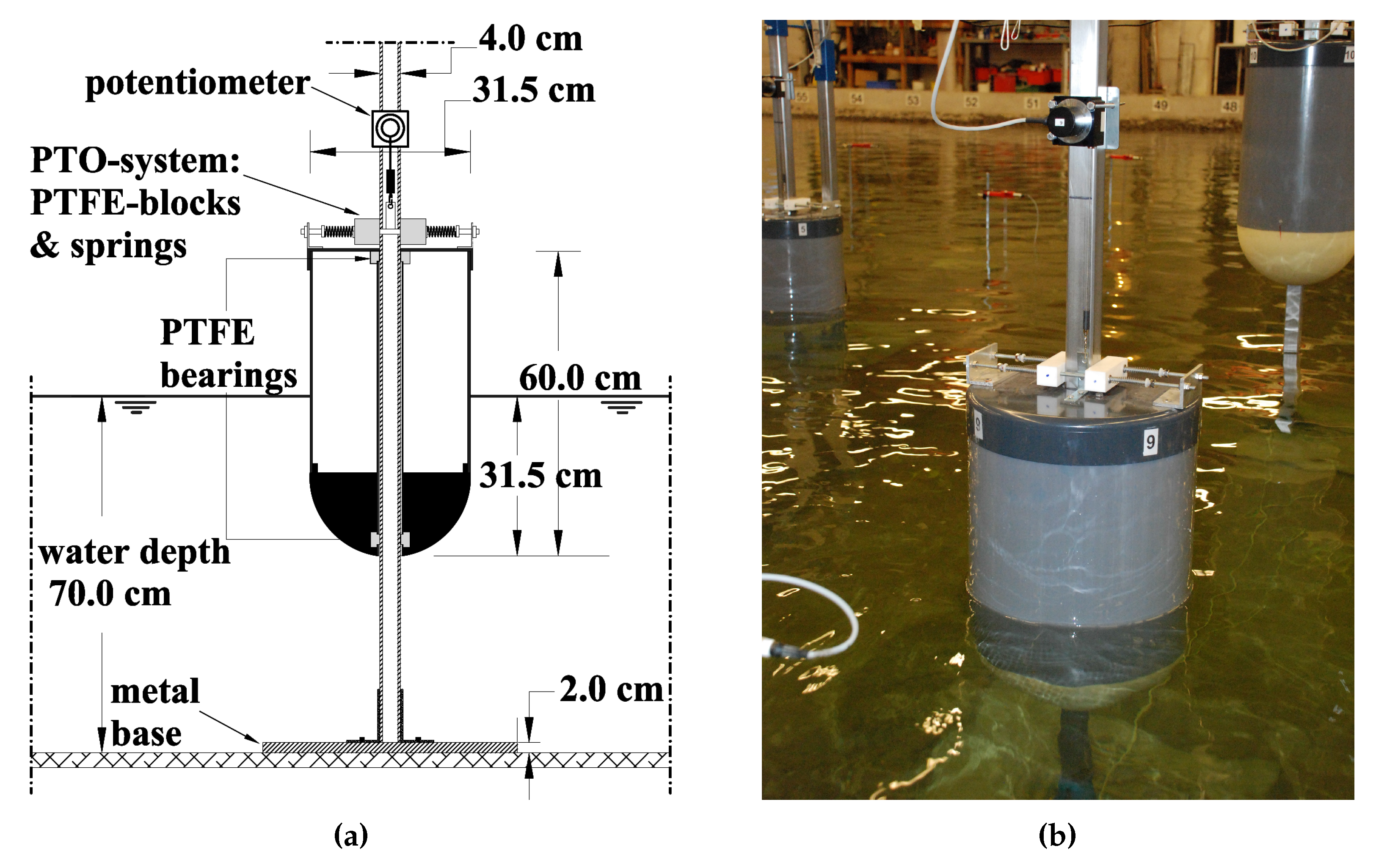
In this work we present numerical results of WEC arrays subjected to non-breaking regular waves representing operational conditions. Validation of these numerical results with experimental data is required prior to survivability simulations of WEC arrays under extreme wave loading with breaking wave events. The ability of our coupled fluid–motion solver to simulate multiple independently moving WECs arranged in different array configurations subjected to regular waves has been demonstrated in [16,17]. In this paper, we extend the comparison study between the numerical results obtained with our coupled fluid-motion solver and the experimental data obtained during the WECwakes project [14,15] for an array of two, five and up to nine WECs. The geometry of an individual heaving FPA type WEC is depicted in Figure 1. Figure 1 also shows the supporting axis which serves as a sliding mechanism to allow solely heave motion of the WEC. A power take-off system is installed on the WEC by mimicking a coulomb damper using friction brakes (composed of two PTFE blocks and four springs) between the floating WEC and the supporting axis. The WECwakes tests focussed on recording WEC responses, forces on WECs and wave field modifications around single WEC units and WEC arrays of 2 up to 25 WECs. The experiments performed in the wave basin at DHI (Denamrk) within the EU FP7 Hydralab IV program are until today the largest experimental setup of this kind worldwide. WECwakes resulted in a comprehensive database which is publicly available for researchers through the Hydralab rules. Not only the WECs’ heave motions but also the surge forces acting on the WECs and the perturbed wave field around the different WEC arrays obtained in a CFD NWT are validated in this paper using the WECwakes dataset.
The remainder of this paper is organised as follows. Firstly, in Section 2, the governing equations for the numerical model are presented, followed by a description of the computational domain, the boundary conditions applied and the solver settings. Subsequently in Section 3, the numerical model is used to perform several simulations while in Section 4 the obtained results are discussed in detail. Finally, the conclusions are drawn in Section 5.
2. Numerical Model
In this section, the numerical model used for simulating WEC arrays inside a CFD NWT is summarised. Subsequently, the computational domain is presented together with the grid characteristics. The last two parts of this section are dedicated to explaining the different boundary conditions and solver settings.
2.1. Coupled Fluid-Motion Solver
The coupled fluid–motion solver is implemented in OpenFOAM®, version 3.0.1 [18]. The governing equations for the fluid and motion solver together with the FSI coupling algorithm are formulated in the following three subsections.
2.1.1. Fluid Solver
The two-phase fluid solver uses the three dimensional (3D) incompressible Reynolds-Averaged Navier-Stokes (RANS) equations to express the motion of the two fluids (i.e., water and air). The RANS equations consist of a mass conservation Equation (1) and a momentum conservation Equation (2) written in Einstein summation notation as:
in which t is the time, () are the Cartesian components of the fluid velocity, is the fluid density, is the effective dynamic viscosity, is the pressure in excess of the hydrostatic. is an external body force (including gravity) which is defined as:
in which the gravitational acceleration vector m/s, is the Cartesian coordinate vector (), is the surface tension tensor term which is neglected in the present study. Note that the mean values for the variables considered are written in terms of Favre-averaging (density weighted) due to the varying density in the NWT.
The interface between water and air is obtained by the Volume of Fluid (VoF) method using a compression term as documented in [19]. The method is based on a volume fraction which is 0 for a completely dry cell and 1 for a completely wet cell and in between 0 and 1 for an interface cell containing both water and air. The volume fraction is solved by an advection Equation (4):
where . In the present study, the default value of equal to 1 is applied.
In a post-processing step, the position of the free water surface is determined by a discrete integration of the volume fraction over a vertical line (Z-direction) divided in n equal parts:
The density of the fluid within a computational cell is calculated by a weighted value based on the volume fraction . The effective dynamic viscosity is obtained by the sum of a weighted value based on the volume faction and an additional turbulent dynamic viscosity :
For the waves studied in this work, the Reynolds () number and the Keulegan-Carpenter () number are equal to and respectively. According to [20], no clear turbulent behaviour is expected around the WECs for those and values. Therefore, in the first instance, only laminar solutions are calculated by setting equal to 0. As shown later on, the main features of the WECs’ heave motions, the surge forces on the WECs and the perturbed wave field are already captured by assuming laminar flow conditions. However, in case turbulence plays a major role (e.g., flow separation due to a non-streamlined WEC geometry or during wave breaking events), we refer to our previous works [21,22] on how to properly deal with RANS turbulence modelling for a two-phase fluid solver by using a buoyancy-modified or turbulence model. A buoyancy-modified turbulence model not only results in a stable wave propagation model without wave damping [21] but it also predicts the turbulence level inside the flow field more accurately in the surf zone where waves break [22].
2.1.2. Motion Solver
The kinematic motion of a rigid body is calculated by a motion solver. During the WECwakes project, the motion of the WECs was restricted to heave only. This allows a reduction from a six to a one degree of freedom motion solver. The motion solver calculates the vertical position z of the body by applying Newton’s second law at the current time :
in which is the overall vertical force (including gravity) obtained with the fluid solver by integrating the pressure and shear forces acting on the body’s surface and is the vertical acceleration of the body. Once the acceleration is known, the vertical velocity and the vertical position during the same time are calculated by a second order accurate Crank-Nicolson integration scheme:
in which n is the previous time, is the current time and is the time step. The new position of the body serves as a boundary condition for the mesh motion operation (see later in Section 2.2).
In order to have a converged solution between the hydrodynamic flow field around and the kinematic motion of a WEC, the following kinematic condition needs to be fulfilled at the interface between the fluid and the WEC:
in which and v are the vertical fluid velocity and the vertical WEC’s velocity respectively. Note that the fluid velocities and are equal to 0 m/s at the fluid-WEC interface because only heave motion of the WEC is allowed.
2.1.3. Coupling Algorithm
The coupling between a fluid and a motion solver in rigid body simulations is done by interchanging the total force acting on the body. In the present study, the fluid solver returns the vertical force acting on the WEC which is calculated as the discrete sum of the pressure forces, viscous forces, the downward weight of the body and all the external forces acting on the WEC:
in which and are respectively the pressure and the shear stress tensor acting on each boundary face around the WEC, is a unit vector normal to the area of boundary face j and m is the dry mass of the WEC. is any external force acting on the WEC such as the power take-off (PTO) system force or the frictional force caused by the sliding mechanism used in the experimental setup (see Figure 1 and further in Section 3).
In order to satisfy Equation (8), the coupling algorithm is applying multiple sub iterations during every time step in the transient simulation. The convergence speed between the fluid and motion solver is enhanced by using an accelerated coupling algorithm derived in previous work of the authors [23], reducing the computational cost in terms of CPU time. For floating bodies with a small added mass effect, such as the WECs considered in this research, a fixed amount of three sub iterations is sufficient to reach convergence of Equation (8) during every time step, see [23].
2.2. Computational Domain
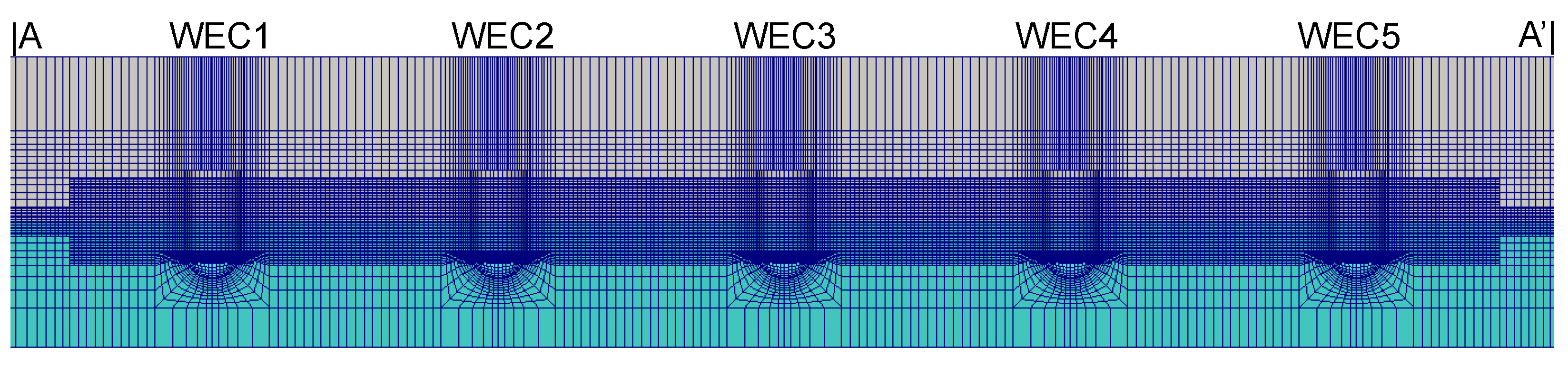
All the numerical simulations are performed in a NWT which represents the experimental wave basin as well as possible. Details regarding the experimental wave basin at DHI have been included in previous work [17]. A plan view of the NWT setup is depicted in Figure 2 showing the WECs’ and wave gauges’ (WG) positions as used during the WEC wakes experiments. In summary, the NWT is represented by a structured grid consisting of only hexahedral cells. In order to limit the number of grid cells in the computational domain, a longitudinal symmetry plane is used along the X-axis. As an example, a longitudinal cross section along the X-axis of the numerical domain for the 5-WEC array is shown in Figure 3. Local mesh refinements are performed in the zones of interest: around the free water surface and around the individual WECs. The vertical grid resolution is 1 cm (≈H/7 in which m is the wave height, see later in Section 3) in the zones of interest, which is sufficient according to [4,17]. The horizontal cell sizes and are equal to 2 cm (≈L/119 in which m is the wave length, see [24]) and increase towards the boundaries of the NWT in order to limit the number of cells and thus also the required computing time. The only exception is that is kept constant towards the inlet boundary in order to properly simulate wave propagation towards the WEC array. Note that properly resolving the boundary layer around the WEC units would require a very fine mesh resolution, resulting in cells with a large aspect ratio. It is known that those type of cells are to be avoided for a VoF-type fluid solver, as they will adversely affect the accuracy of the free surface position. Furthermore, for the simulations presented in this work, pressure forces acting on the WEC will dominate over viscous effects with respect to the wave-induced WEC’s heave motion.
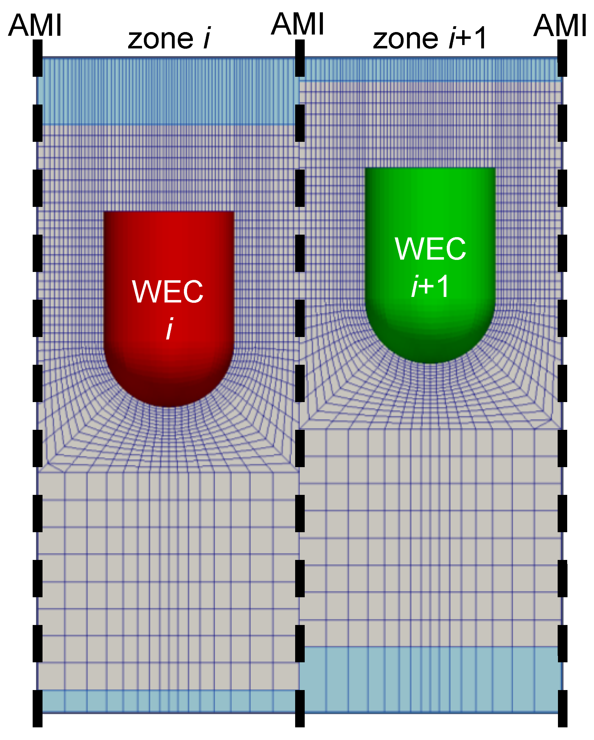
In order to simulate multiple independently moving WECs in an array configuration, arbitrary mesh interfaces (AMIs) are implemented in order to create sliding meshes (see dashed vertical lines in Figure 4 for the case of two WECs). These AMIs define a zone of cells around each WEC. In each zone, only the lowest and highest row of cells (see blue shaded boxes in Figure 4) are expanded or compressed according to the motion of the WEC located in that zone. This methodology is implemented to prevent undesirable mesh deformations around the interface between water and air (i.e., high non-orthogonality and skewness of the computational cells). As a disadvantage, high aspect ratios are obtained for the distorted cells. However since those cells are not inside the zones of interest, it does not affect the accuracy of the simulations. All the variables solved with the fluid solver, such as velocity, pressure and volume fraction, are interpolated over the AMIs.
2.3. Boundary Conditions
The bottom and side wall of the NWT are modelled as a solid wall: a Dirichlet boundary condition is set for the velocity (0 m/s in the three directions) while the pressure and volume fraction are set to a Neumann condition. At the inlet and outlet, wave generation and absorption are implemented using the IHFOAM toolbox [25,26]. On all the boundary faces of each WEC, the velocity vector is set to a moving wall condition (see Equation (11)) and the pressure and volume fraction are set to a Neumann condition. The atmospheric conditions at the top of the numerical domain are set to a mixed Dirichlet-Neumann boundary condition for the velocity, pressure and volume fraction.
2.4. Solver Settings
For all the simulations presented, the following solver settings are used: central discretisation for the pressure gradient and the diffusion terms; total variation diminishing (TVD) schemes with a van Leer limiter [27] for the divergence operators; second order implicit time discretisation; a maximum Courant number equal to 0.3 as recommended in [23] for FSI simulations using a VoF method.
3. Results
In this section, we present numerical simulations of three different WEC array configurations subjected to regular waves. An overview of the employed benchmark data, both numerical and experimental results, is summarised in Table 1. In this study, the underlined tests and results are presented and validated using the experimental WECwakes dataset. The other results, i.e., the free decay tests, have been reported in previous works [16,17]. For the 2-WEC and 5-WEC array, a simulation with fixed WECs is also performed in which the WECs are not moving. Subsequently, more challenging simulations are presented in which the heave motion is allowed for a 2-WEC, 5-WEC and 9-WEC array in response to an incident regular wave train. For each test, the waves have a height H equal to m, a wave period T of s and are generated in a water depth d of m. At the inlet of the numerical wave tank, waves are generated using a second order Stokes theory and active wave absorption is turned on. Each numerical simulation ran for 50 s to obtain a sufficiently long dataset after the warming-up phase but only the last 10 s are shown. The numerical results are validated by using experimental data for the WECs’ heave motions, the surge forces on the WECs and the surface elevations in the wave tank. The relative error between the numerical result (num) and the experimental result (exp), in percent, is defined as:
in which is representing the heave motion, surge force or surface elevation. The maximum and minimum values for observed in the time signals are averaged between s and s. The numerically computed values for the error, Equation (13), are presented in Table 2.
3.1. 2-WEC Array
In this first subsection, two WECs in line are modelled in the NWT (WEC4 and WEC5 in Figure 2). The distance between the WECs’ centre is equal to five times their diameter ( m), see Figure 2. Firstly, the WECs are kept fixed in their equilibrium position and no motion is allowed. Secondly, the WECs are allowed to heave in response to the incident waves.
3.1.1. Fixed 2-WEC Array
If the WECs are kept fixed, the incident wave field is perturbed by wave reflection and wave diffraction. The purpose of this particular test is to check the reproduction of the perturbed wave field in a numerical model without considering the wave field modification by the WECs’ heave motion (i.e., radiated wave field around each WEC).
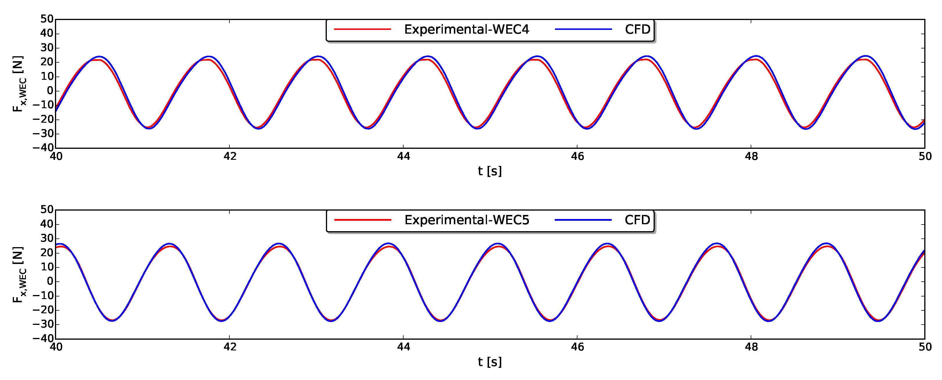
Figure 5 presents the wave-induced surge (horizontal) forces acting on WEC4 and WEC5 as a function of time. The red line indicates the experimental data while the blue line depicts the numerically obtained force by the CFD fluid solver. Note that the noise in the time signals of the experimental force measurements has been filtered out using a bandpass filter. An outstanding agreement is observed between the numerical and experimental data which is also confirmed in Table 2 by relative errors equal to 7% and for WEC4 and WEC5 respectively. This achievement is a necessary requirement for the simulations with heaving WECs later in this study because the wave-induced force acting on a floating body determines its kinematic motion.
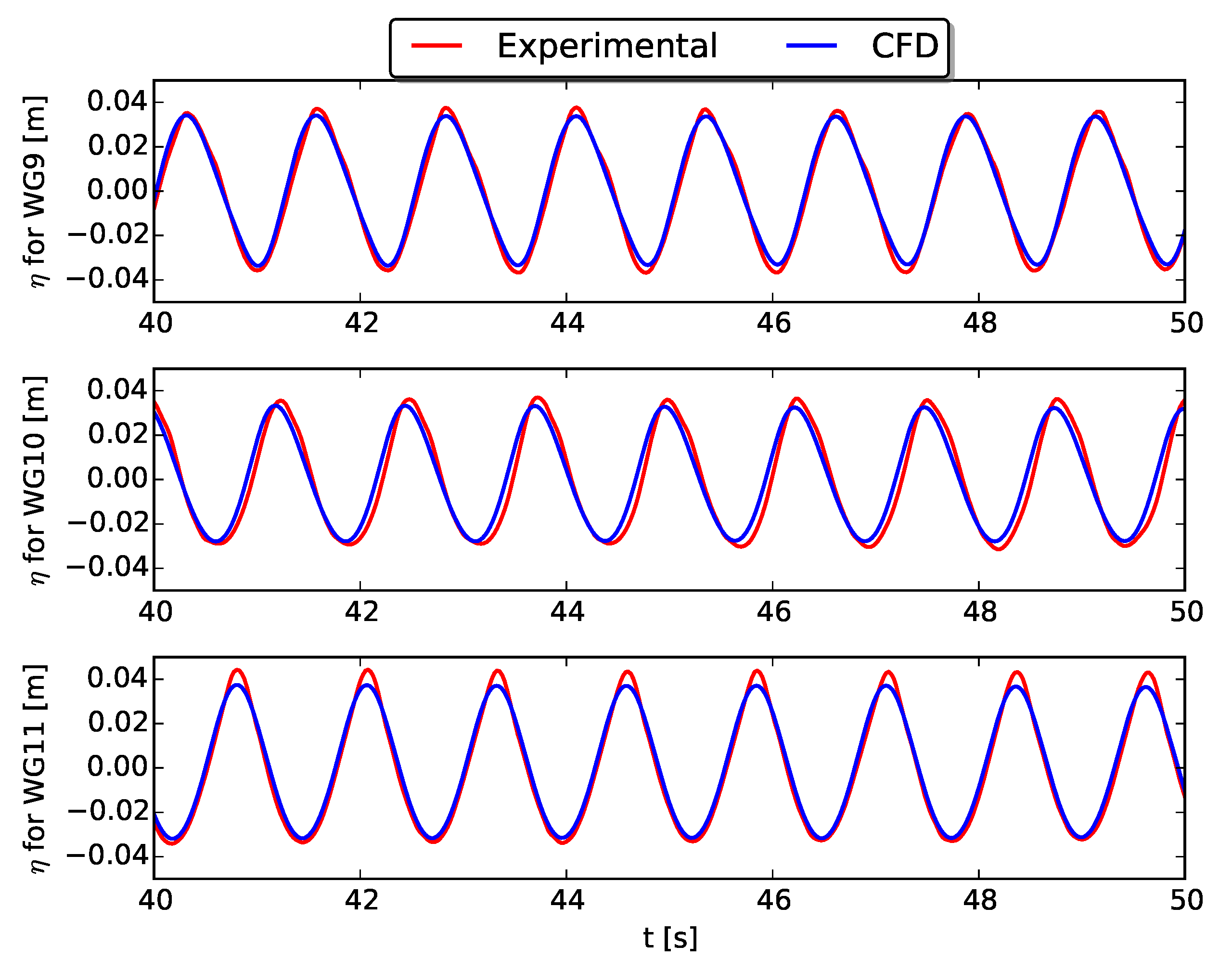
The perturbed wave field due to reflection and diffraction is visualised in Figure 6 by the surface elevations at three locations in the NWT: WG9, WG10 and WG11 (see Figure 2). Again, the red lines indicate the experimental measurements and the blue lines are the processed time series of the surface elevations in the NWT (Equation (5)). For WG9, before the 2-WEC array, and WG10, behind the 2-WEC array, an identical signal is observed between numerical and experimental data (see Table 2 for the relative errors). However, for WG11 further behind the 2-WEC array, small discrepancies between numerical and experimental data are visible in the maximum and minimum surface elevation (relative error of ) but the wave phase is similar. It is also observed that the wave height is the same for the three wave gauges in the NWT and equal to m which is slightly smaller than the incident wave height equal to m. It is remarkable that this is not the case for the experimental records, which show an increased wave height for WG11. We expect however that due to the slender geometry of the WECs, wave diffraction is not significant and no wave field modification is present at the position of WG10 and WG11 behind WEC5. This is indicated by Figure 3.20a in [24] which presents a cross section of the incident and diffracted wave fields’ amplitude for a fixed single WEC unit obtained with the BEM solver WAMIT.
3.1.2. Heaving 2-WEC Array
In this section, the two WECs are allowed to heave in response to the incident regular waves. The incident wave field is not only perturbed by diffracted and reflected waves but also by radiated waves generated by the heave motion of the WECs. For heaving WECs, the perturbed wave field is thus a combination of incoming, diffracted, reflected and radiated waves. The radiated wave field has been validated separately in previous work [17] by simulating a free decay test of these WECs. It was concluded that the correspondence between numerically and experimentally obtained surface elevations is good despite the small wave amplitudes of the radiated wave field. However, internal friction caused by the sliding mechanism between the WEC and the vertical supporting axis through internal contact points during the experiments (see Figure 1a) requires attention to correctly include it in a CFD model for validation studies. Therefore the following two measures are undertaken to simulate the studied heaving WECs subjected to regular waves. Firstly, the WEC’s mass is modified and a linear damper is needed to account for the internal friction due to the sliding mechanism used in the experiments (cfr. viscous flow of water between the shaft and shaft bearing, see Figure 1a). The method is described in [4] and is based on tuning the WEC’s heave motion to the experimental measurement for a free decay test. The linear damper is formulated by an additional frictional force on the WEC:
in which c is the damping coefficient equal to 4.86 kg/s, as calculated in [17] by validating a free decay test using WEC5 and is the WEC’s vertical velocity. Secondly, the incident waves push the experimental WECs against their sliding mechanism (cfr. a coulomb damper [17]), resulting in an additional frictional force:
in which the coefficient of friction and is the horizontal force in the X-direction acting on the WEC.
For this test case, a PTO system is activated on both WECs to extract energy out of the incident wave field (see Figure 1a). The PTO system used in the experiments is modelled as a second coulomb damper [17]:
in which the spring compression increment mm and the spring stiffness coefficient N/mm.
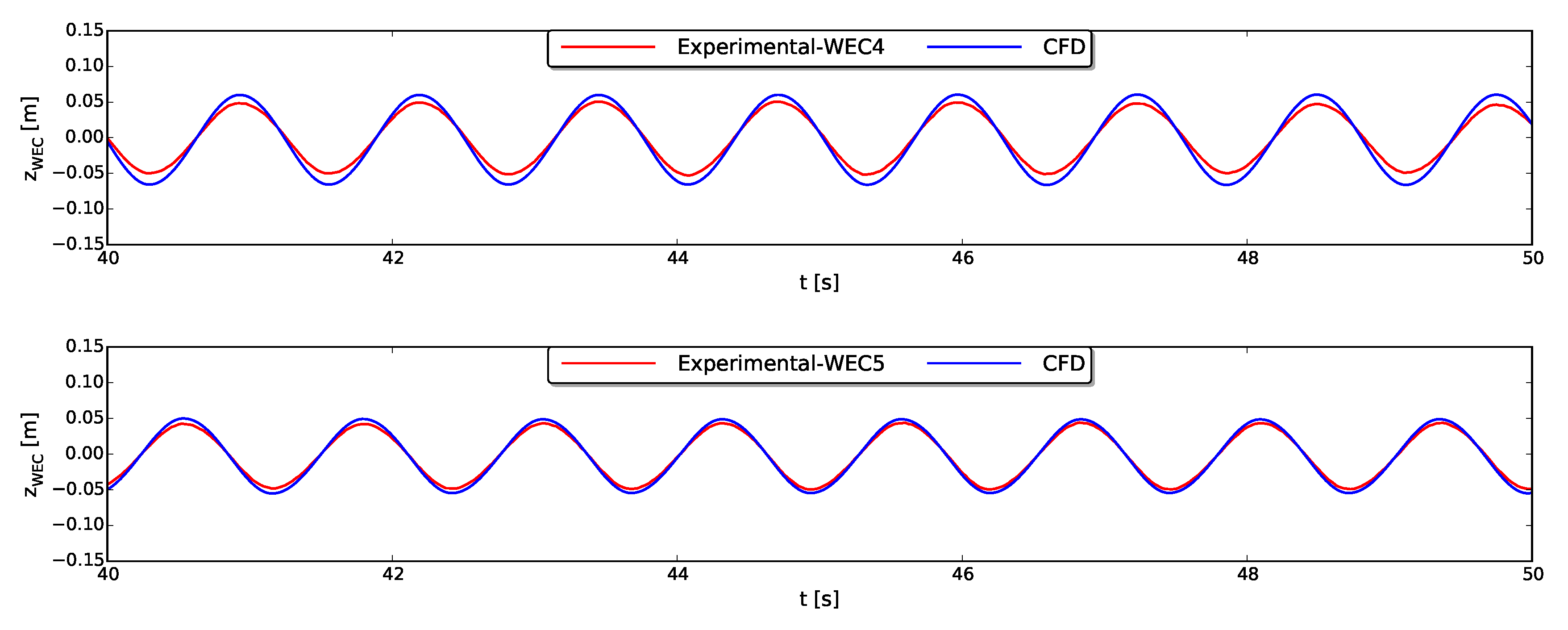
Figure 7 shows the time series of the WECs’ heave motions for both numerical and experimental data and in general a good correspondence is observed. The shape and the phase of both time signals are similar while the differences in heave amplitudes are limited. For the experimental signals, the maximum heave amplitude of WEC4 ( m) is only slightly larger than that of WEC5 ( m) while the numerically obtained results show larger differences: m and m for WEC4 and WEC5 respectively.
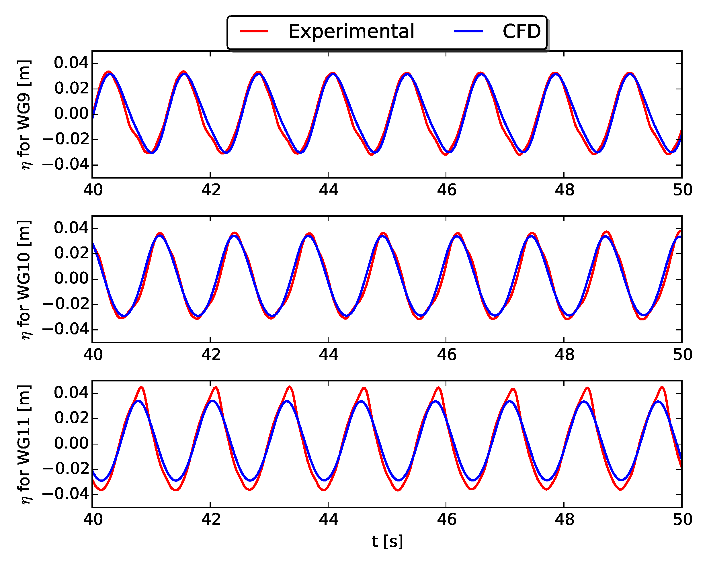
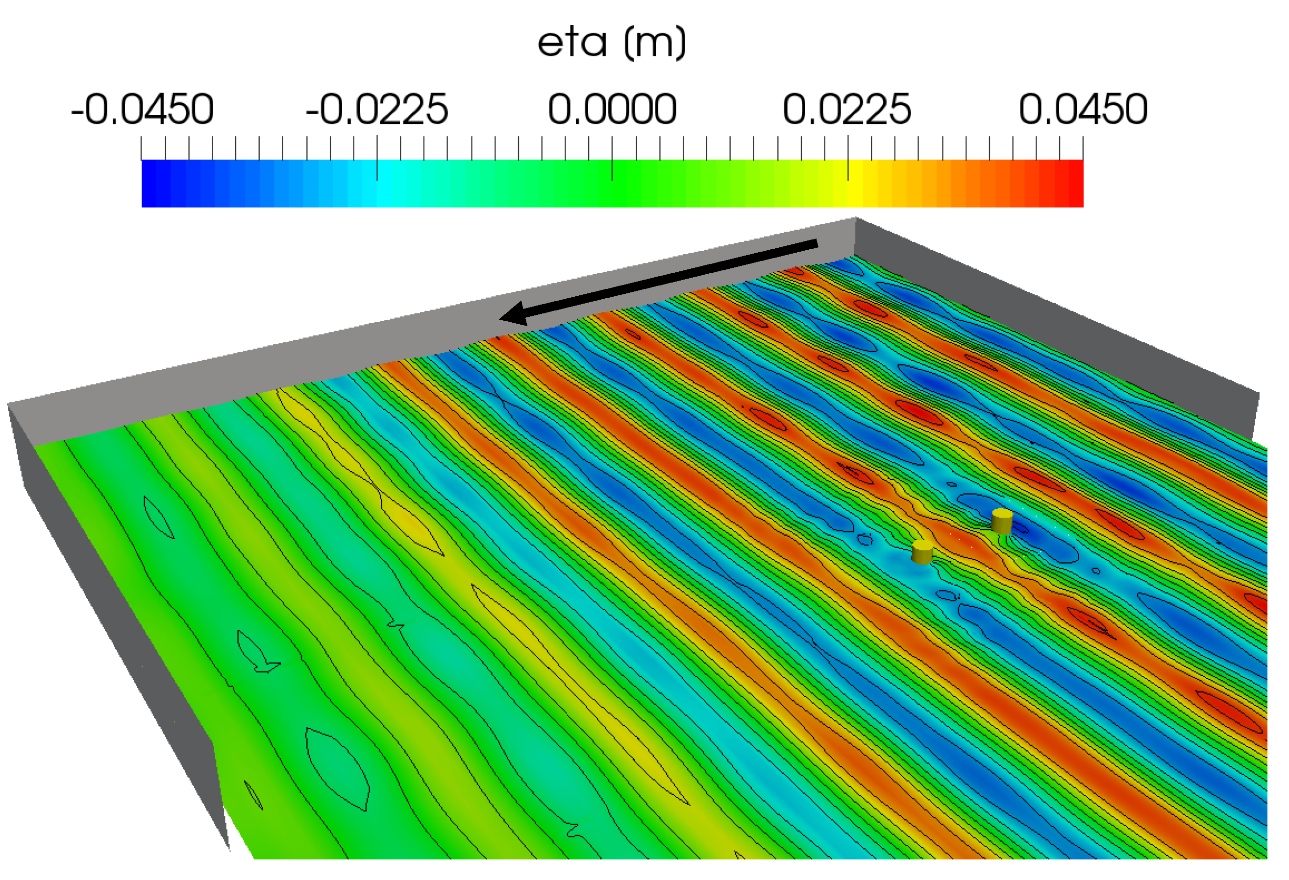
The time series of the surface elevations are presented in Figure 8. Differences between numerical and experimental signals are observed for the minimum and mainly for the maximum surface elevations. The largest relative error is again observed for WG11, which was also the case for the fixed WECs simulation presented in Figure 6 (see Table 2). Figure 9 depicts a snapshot of the perturbed wave field at s inside the NWT. Waves are generated and absorbed at the right and left boundary respectively. The observed reduced wave height behind the 2-WEC array near the outlet boundary is due to the increasing aspect ratio of the grid cells as reported in Section 2.2. This increasing aspect ratio is responsible for numerical wave damping. This is however beneficial in order to avoid wave reflection from the absorbing outlet boundary. Only in a limited area around the 2-WEC array, a significantly perturbed wave field is observed in the NWT. The wave gauges used in Figure 8 are however outside that zone which explains the identical wave height in the NWT at those three locations. Due to the perturbed wave field near the WECs, each WEC is slightly influencing the numerically predicted heave motion of the other WEC which shows the interaction between the two WECs. This is also illustrated in Figure 7 by observing a different amplitude of the numerically obtained heave motions for both WECs.
3.2. 5-WEC Array
In this subsection, three more WECs are added to the NWT resulting in an array of five WECs installed in a line: WEC1 to WEC5 (see Figure 2 and Figure 3). Again, numerical and experimental results are presented using both fixed and heaving WECs subjected to regular waves.
3.2.1. Fixed 5-WEC Array
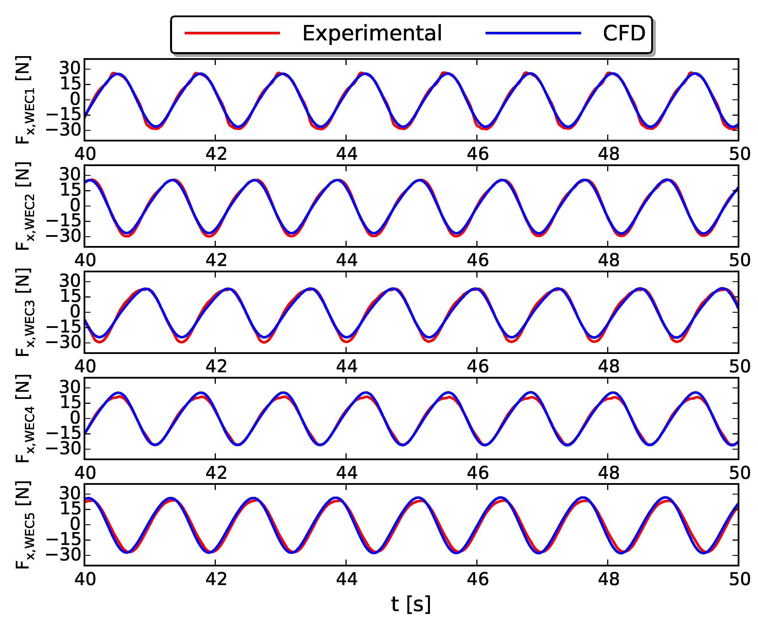
Figure 10 depicts the wave-induced surge force on the five fixed WECs as a function of time for both numerical (blue lines) and experimental data (red lines). Again, the numerically obtained surge forces are in a very good agreement with the experimental data and show relative errors of maximum in Table 2. The time signals also reveal that the maximum and minimum surge force on the WECs is independent of the WEC’s position in the array and wave basin. This is also confirmed by comparing Figure 5 (2-WEC array) and Figure 10 (5-WEC array) showing identical loading cycles on the fixed WECs.
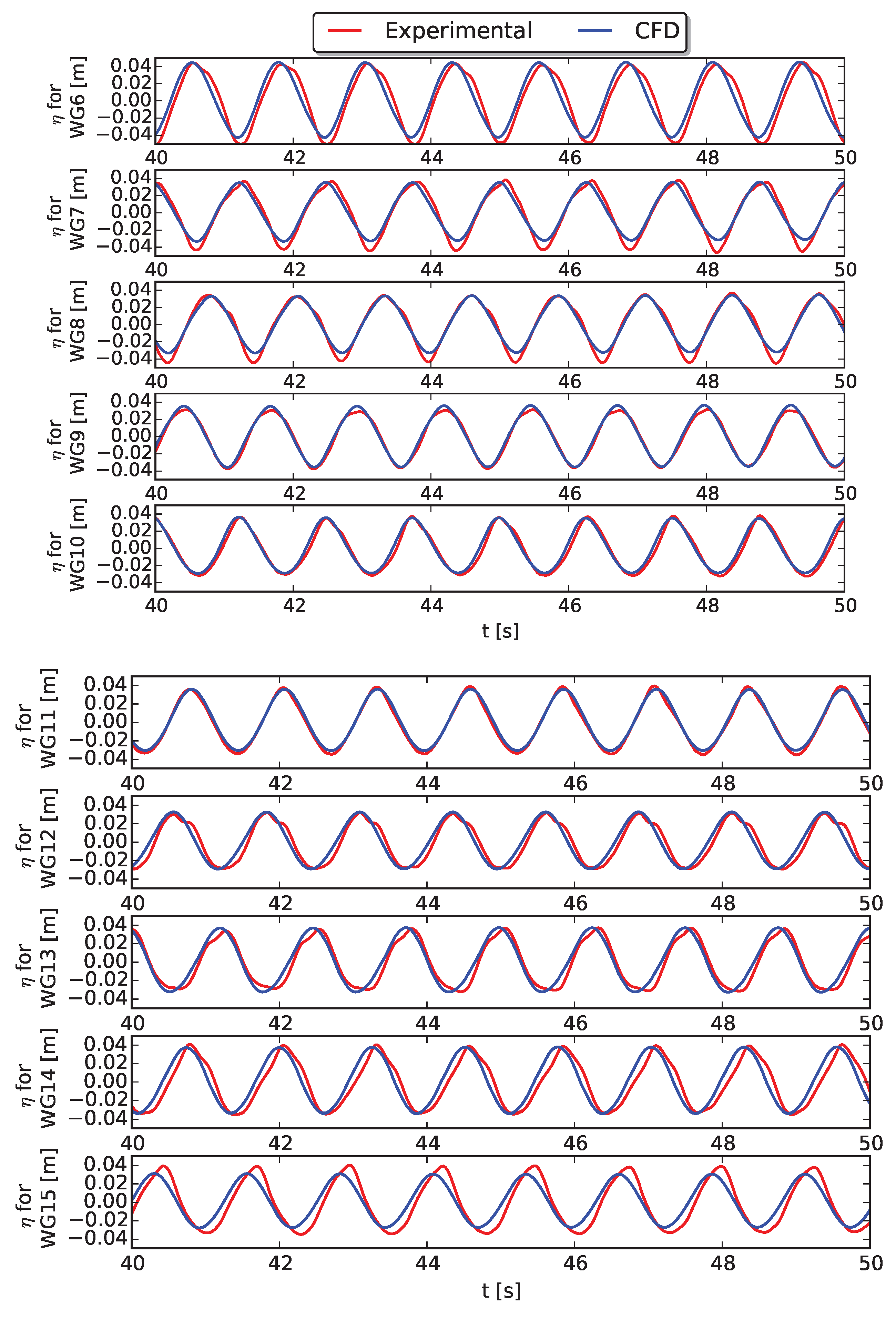
The perturbed wave field due to the presence of fixed WECs is visualised by using time series for the surface elevations in Figure 11 at different locations in the NWT (see Figure 2). The numerical results are in a very good agreement with the experimental measurements, except for WG8 and WG11 (see also the larger relative errors in Table 2 compared to the other WGs). Similar to the observation for the fixed 2-WEC array (Section 3.1.1), a larger amplitude of the experimentally obtained surface elevations for WG11 is observed compared to the numerical results. For this test case, wave gauges were also installed in between the WECs, see Figure 2. For WG6 to WG9, Figure 11 indicates a small perturbed wave field due to reflection and diffraction: WG6: m (reflection only), WG7: m, WG8: m and WG9: m. Next to the array (WG12, WG13, WG14 and WG15), no disturbance is observed in the time signal of the surface elevations because those wave gauges are located outside the zone of a significantly perturbed wave field.
3.2.2. Heaving 5-WEC Array
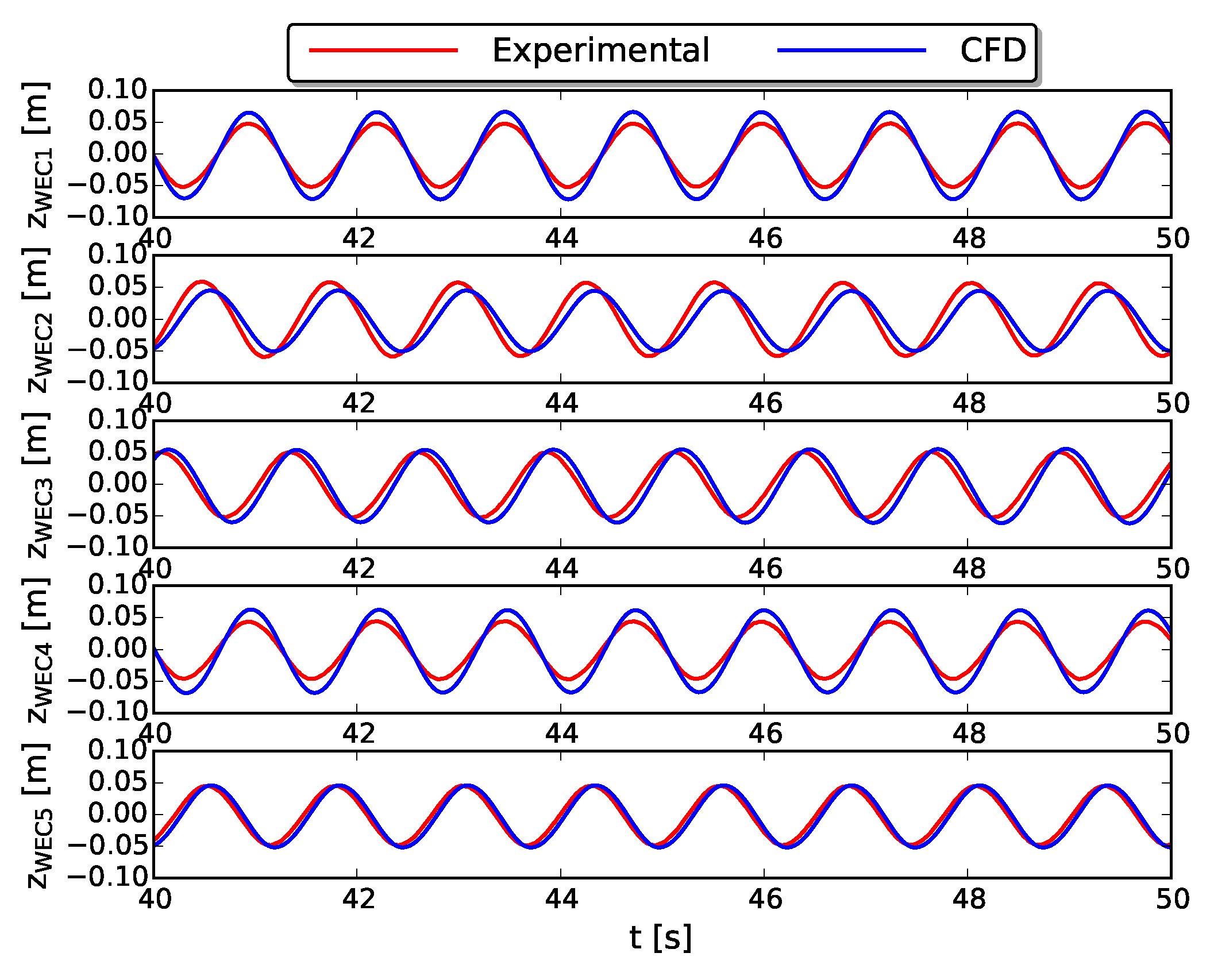
If the WECs are allowed to heave, three frictional forces (, and ) are applied on each WEC with identical parameters as for the 2-WEC array described in Section 3.1.2. The heave motions of the five WECs as a function of time are given in Figure 12 for both experimental and numerical data. The time series reveal that, in general, both results are comparable. However, significant differences in heave amplitudes are observed for WEC1 and WEC4 with relative errors larger than (see Table 2). Remarkably for WEC2, the numerically predicted heave motion shows a small phase difference with the experimental data. Those discrepancies are discussed in Section 4.
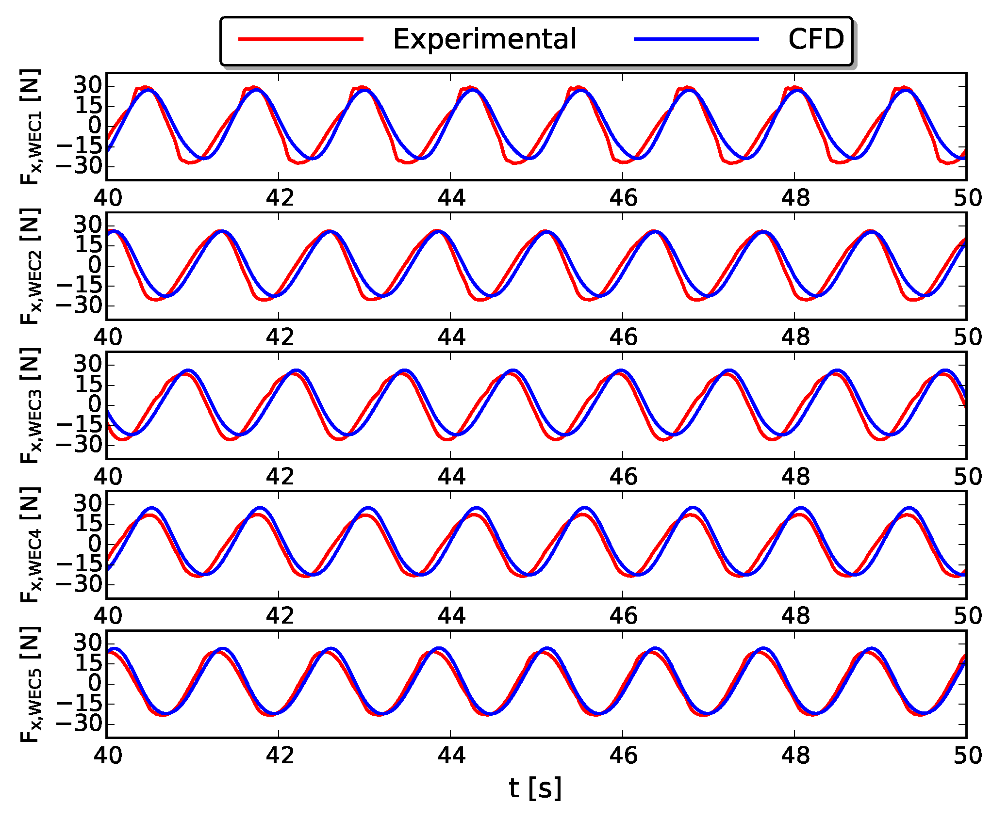
Figure 13 depicts the wave-induced surge force acting on the WECs for both experimental and numerical data. In contrast to the discrepancies observed for the WECs’ heave motions, a better agreement between numerical and experimental data is demonstrated for the surge forces on the WECs. However, for WEC1, the peaks and troughs in the experimental signal are deviating from the numerical result. This is due to large spikes observed in the experimental recorded time series before noise filtering is applied.
A good agreement is also found when comparing numerical and experimental data for the perturbed wave field around the 5-WEC array (Figure 14). However, some discrepancies are observed regarding the time series of the surface elevations in the wave basin, in particular for the maximum and minimum surface elevations. Figure 15 depicts a snapshot of the perturbed wave field at s. Similar to Figure 9, waves are generated and absorbed at the right and left boundary respectively. Again, the reduced wave height behind the 5-WEC array near the outlet boundary is due to the increasing aspect ratio of the grid cells leading to numerical wave damping. In a local zone near the array, a significantly perturbed wave field is predicted by the numerical model. Due to a perturbed wave field near the array, the numerically predicted heave motions for the individual WECs are not uniform (see the blue lines in Figure 12). Furthermore, an important reduction in wave height is observed right behind the array.
3.3. 9-WEC Array
The last test presented in this paper uses an array consisting of nine WECs arranged in a 3 × 3 layout. By using the symmetry plane shown in Figure 2, only six WECs are modelled: WEC1 to WEC3 and WEC6 to WEC8. Again, the same frictional forces are applied as previously defined in Section 3.1.2 (, and ). In addition for WEC6, WEC7 and WEC8, an extra coulomb damper is implemented in order to take into account the frictional force of the bearings on the supporting axis (see Figure 1) in the Y-direction into account (cfr. Equation (15)):
where is the horizontal force in the Y-direction acting on the WEC.
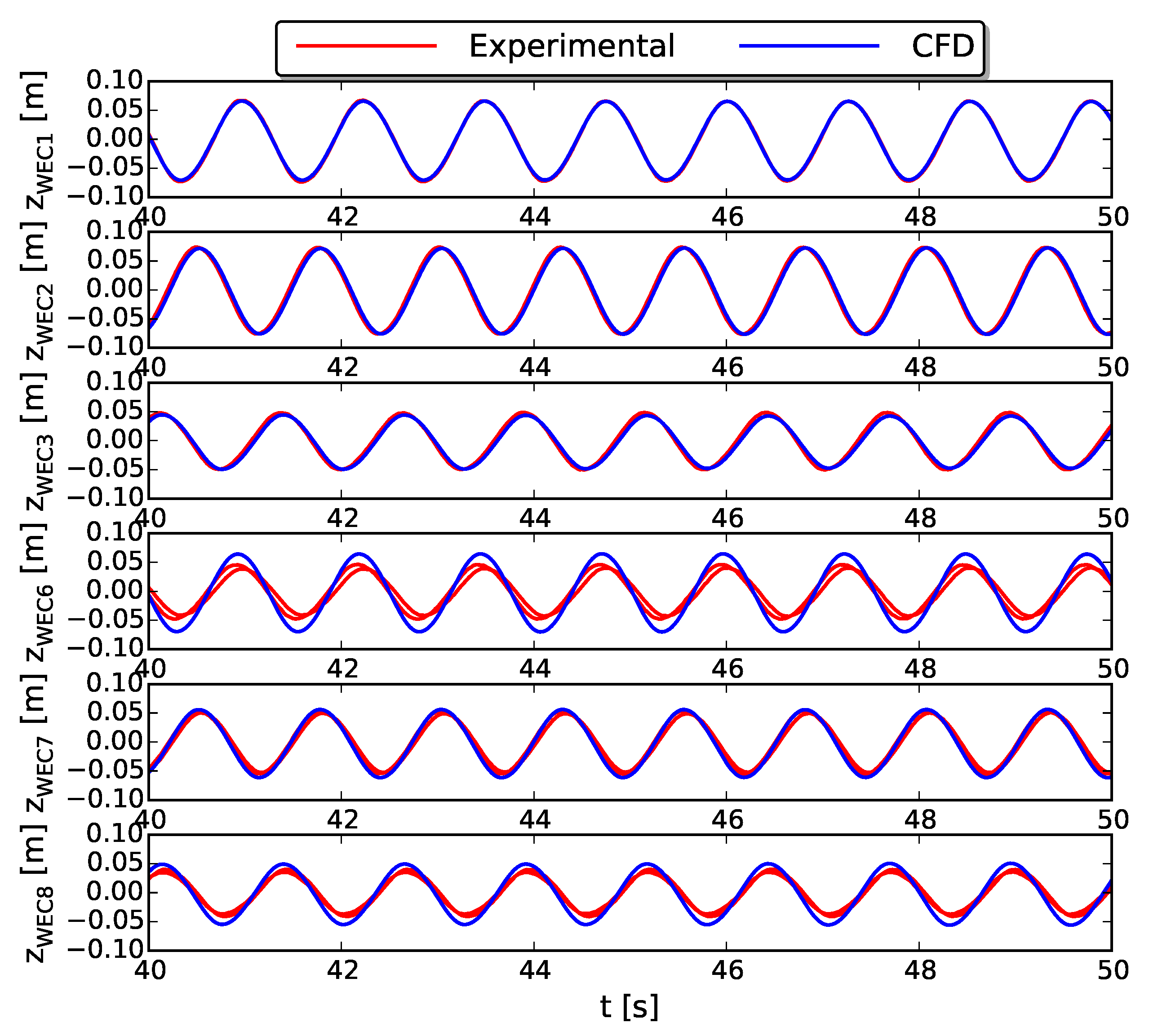
The heave motions for the six WECs are depicted in Figure 16. For WEC6 to WEC8, the experimental signals for WEC11 to WEC13 (see Table 1) are also shown in red. Those two time series are very similar and indicate a symmetrical behaviour for the experimentally obtained heave motions. For WEC1 to WEC3, installed on the symmetry plane, an identical result is observed between the experimental and the numerical model (low relative errors in Table 2). However for the outer WECs (WEC6 to WEC8), larger amplitudes are observed for the numerical result compared to the experimental data resulting in significant relative errors equal to , and respectively. Probably, larger frictional forces were acting on WEC6 to WEC8 during the experiments.
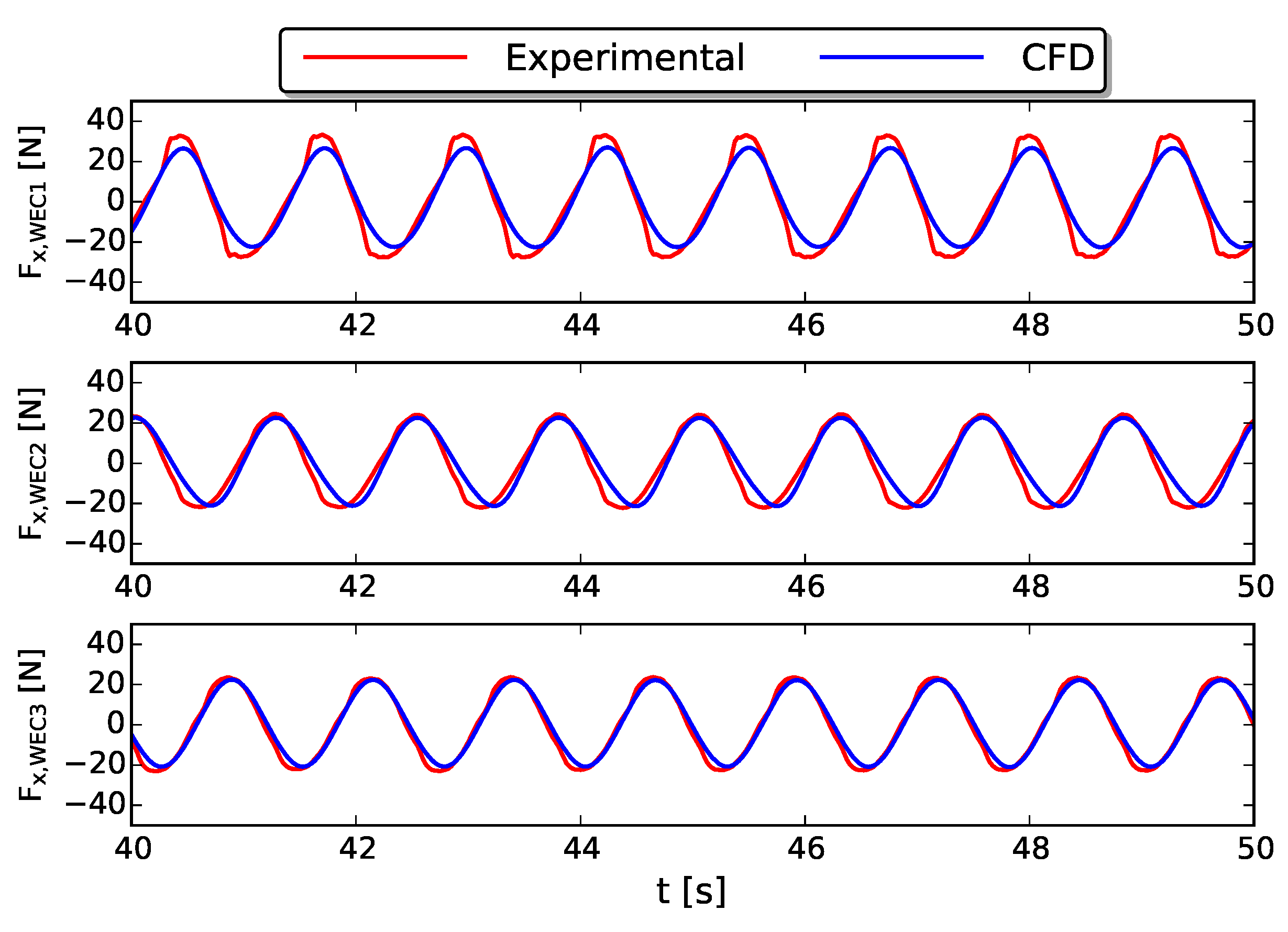
The wave-induced surge forces acting on WEC1 to WEC3, installed on the symmetry plane, are presented in Figure 17 for both the experimental and the numerical model. A good comparison is found between the results but again for WEC1, the peaks and troughs in the experimental signal are deviating from the numerical result due to large spikes observed in the experimental measurements before applying a bandpass filter.
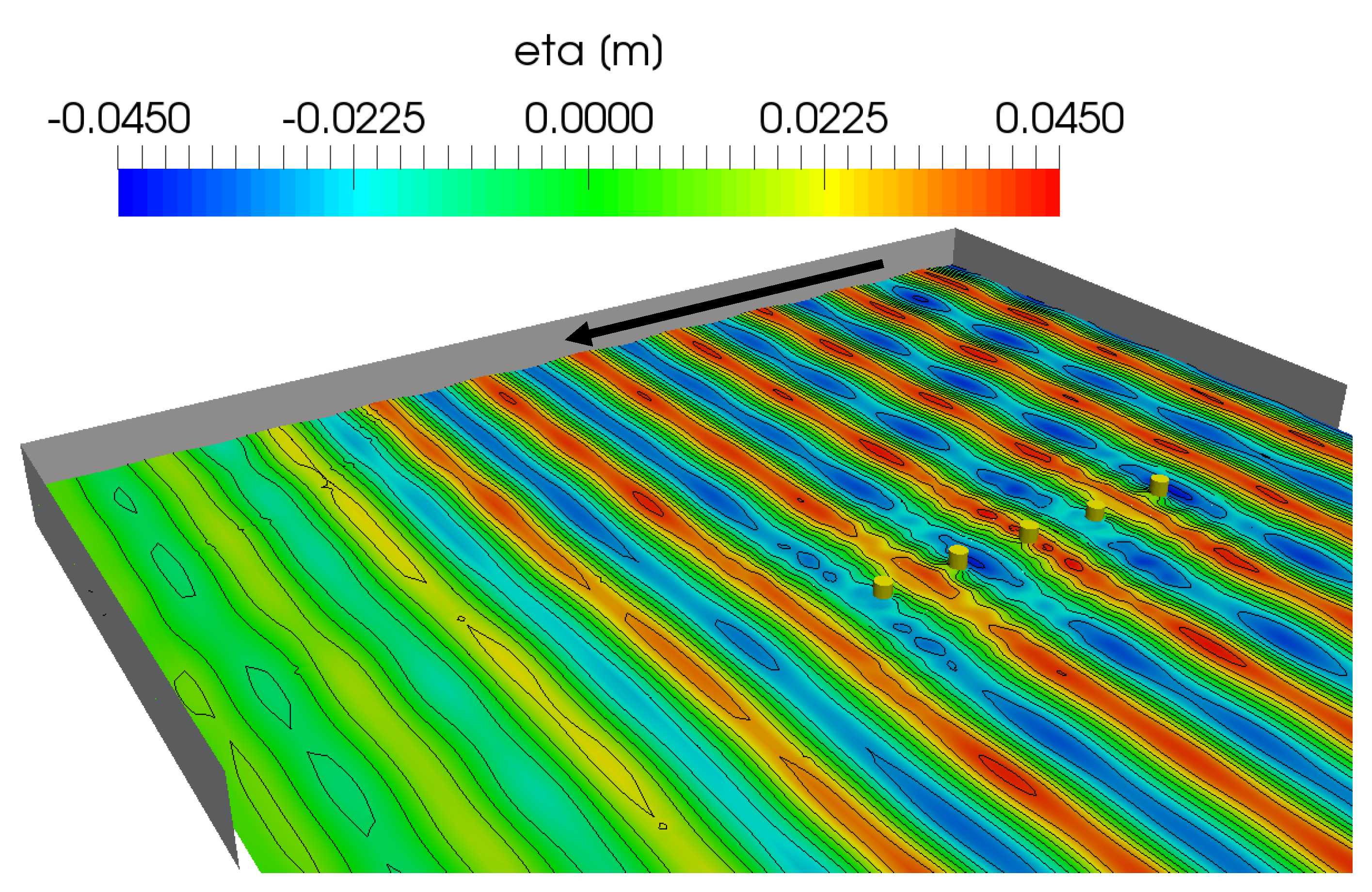
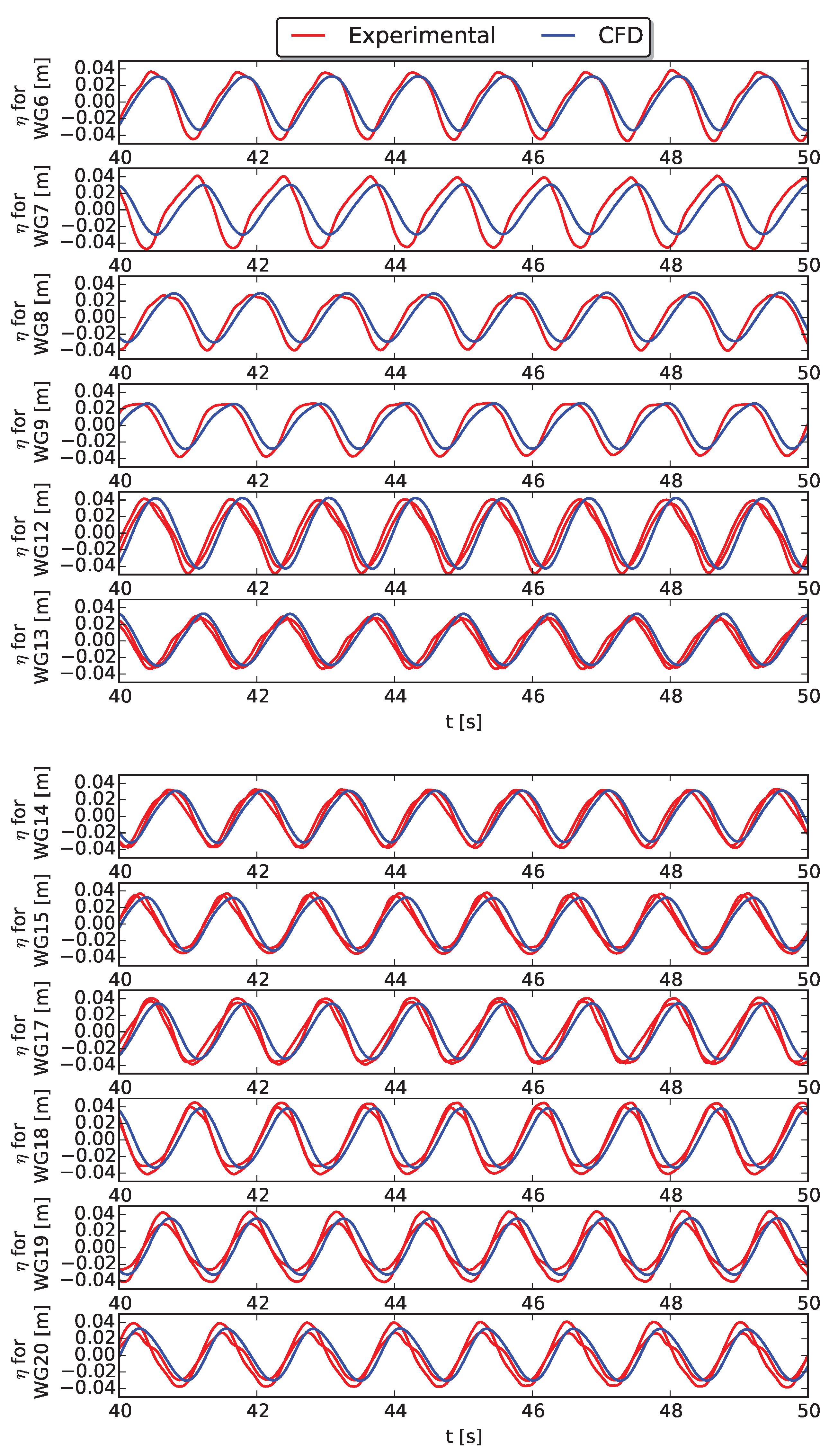
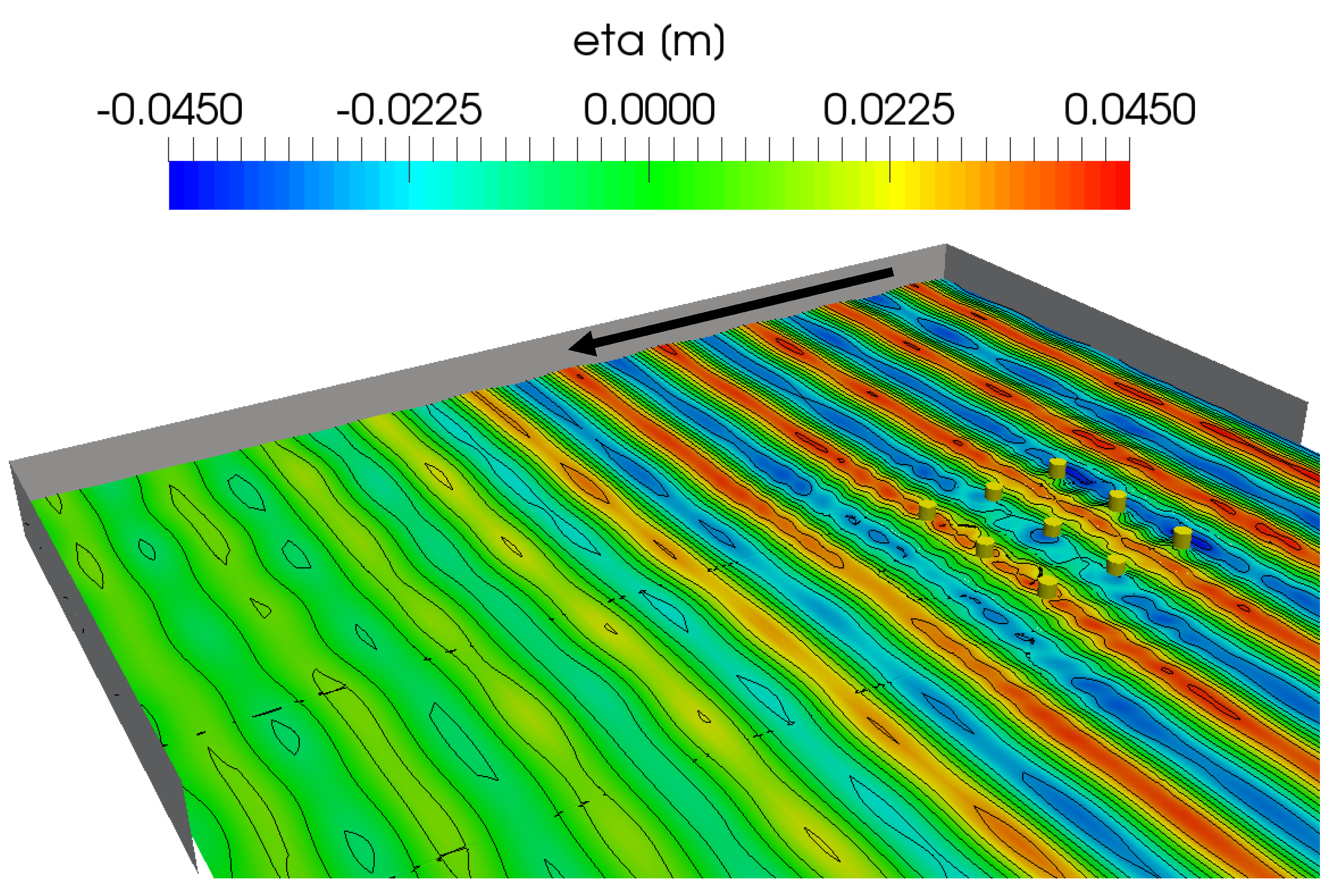
The experimentally and numerically obtained perturbed wave field around the WECs are visualised in Figure 18 using several wave gauges (see Figure 2). Only the wave gauges positioned close to the 9-WEC array are presented. For the wave gauges which are not on the symmetry plane, two experimental results are shown. Only for WG18, WG19 and WG20, a slightly asymmetrical wave field is observed inside the experimental wave basin. In general, except for WG7, a good agreement is obtained between both models taking into account the remarks reported in Section 3.1.2 and Section 3.2.2. In particular for WG18, WG19 and WG20, the numerical result lies in-between the two experimental lines with a small phase shift. Figure 19 depicts a snapshot of the perturbed wave field at s. In a large area around the 9WEC array, a significantly perturbed wave field by the heaving WECs is clearly visible. Due to the larger width of the array, compared to the 2-WEC and 5-WEC array (in a line), a clear reduction in wave height is visible behind the array, which is also observed in Figure 18 for WG9.
4. Discussion
In Section 3, two types of differences between the numerical and experimental results are observed. The first type of differences is seen in the heave motions of the WECs. In this work, we tried to capture as much physics as possible in the numerical model to reproduce the experimental tests. The WEC’s PTO system and the sliding mechanism (see Figure 1) are included by mathematical models to take into account their influence on the WECs’ kinematic motion. During the WECwakes experiments, the PTO system was mimicking a coulomb damper and is thus initially implemented in the numerical model as a coulomb damper only. The sliding mechanism was incorporated by both a linear damper (viscous flow of water between the shaft and shaft bearing) and a coulomb damper (caused by the wave induced horizontal force). However in our previous work [17], we found that the PTO system is not only behaving as a coulomb damper but also partially as an additional linear damper. Furthermore, in reality, friction behaves uncontrolled. For example, during the WECwakes project, it is noticed that the friction characteristics change due to fouling of the supporting axes for the sliding mechanism. Therefore, before each testing day, the supporting axes were cleaned in order to minimise that particular model effect. This highlights partially the unknown physical behaviour of frictional forces in the experimental model. Furthermore, the frictional forces caused by the sliding mechanism might vary over the different WECs within the array. This is probably the most important explanation for the large variation in relative errors obtained for the heave motions over the different WECs, as indicated in Table 2. Note that in this study, identical parameters were used to model the frictional forces on all the WECs based on tuning the numerically obtained heave motion to the experimental measurement during a free decay test using WEC5. In order to perform a validation study of fluid-structure interaction simulations of floating heaving WECs, we recommend to start with validating a free decay test for each individual WEC within the array by using experimental data. This allows the estimation of frictional forces due to a possible sliding mechanism by computing the hydrodynamic parameters of the device (e.g., the damped natural frequency and the hydrodynamic damping coefficient).
The second type of differences is found in the surface elevations of the perturbed wave field. Those deviations are largely assigned to the difference in reflection between the experimental wave basin (with an absorbing beach) and the numerical wave tank (with a shallow water absorbing boundary condition). Additionally, differences between experimental and numerical data are possibly caused by model effects in the experimental setup and numerical errors in simulations presented. For example, small errors in the calibration of the wave gauges contribute to the overall error observed in the experimentally obtained surface elevations. Interestingly, the surface elevations around the WECs are showing smaller relative errors compared to the heave motions (see Table 2). Presumably, they are less influenced by the frictional forces acting on the WECs due to the sliding mechanism used for the experiments.
In general, a very good comparison is found for the horizontal wave-induced surge forces acting on the WECs, as indicated by the relative errors always smaller than , except one, in Table 2. We expect that the surge force is not influenced by the sliding mechanism and consequently does not depend on the frictional forces modelled by the coulomb damper and the linear damper in the numerical model. In order to run simulations with more degrees of freedom (e.g., surge motion), a good prediction of the surge force is required for example.
Despite the observed inaccuracies, in general, the numerical results are in good agreement with the experimentally obtained measurements. In contrast to the experimental data, which are only available at discrete locations, the numerical model yields a much higher spatial resolution of the perturbed wave field inside and around the WEC (array). During the validation of the numerically obtained surface elevations using the experimental measurements, a significantly perturbed wave field is not always observed at those specific locations. Snapshots of the surface elevations inside the numerical wave tank indicate that a significantly perturbed wave field is only observed very close to the WECs where no experimental wave gauges were installed. As a result, the WEC array effects are much easier to identify using the validated numerical wave tank.
5. Conclusions
Numerical simulations of two, five and nine heaving FPA WECs installed in a geometrical array configuration inside a numerical wave tank using CFD have been presented. The simulation results show the capability of state of the art numerical models, including stable coupled fluid–motion solvers, to accurately predict the independent motion of closely-spaced WECs in response to an incoming wave field. As such we are able, as a worldwide pioneering result, to simulate an array of nine independently moving WECs in a numerical wave tank using CFD. The numerically obtained results are validated using the WECwakes dataset. A good agreement is demonstrated for the WEC’s heave motion, the wave-induced surge force acting on the WECs and surface elevations of the perturbed wave field at the measured locations. While results are perfect for the WECs on the symmetry plane of the numerical wave tank, deviations are noticed for the outer WECs, which we attribute to inaccuracies in the estimation of the frictional forces caused by the sliding mechanism of those particular WECs. In general, the numerical results have shown that our coupled fluid-motion solver is a robust and suitable toolbox to study fluid-structure interaction of WEC arrays, making it a complementary tool to experimental model tests. This research opens up the possibilities for numerical simulations of any kind of floating structure installed in any sea state using a numerical wave tank.
Acknowledgments
The first author is Ph.D. fellow of the Research Foundation—Flanders (FWO), Belgium (Ph.D. fellowship 1133817N). The WECwakes project has been funded by the EU FP7 HYDRALAB IV programme (contract no. 261520). The project is a consortium of seven European partners coordinated by Ghent University-Belgium (Peter Troch; Vasiliki Stratigaki). The construction of the WEC models at Ghent University (research grant FWO-KAN-15 23 712 N) and part of the data pre- and post-processing (Ph.D. funding grant of Vasiliki Stratigaki and research project no. FWO-3G029114), have been funded by the Research Foundation—Flanders, Belgium (FWO).
Author Contributions
Brecht Devolder set up the numerical wave tank to study WEC arrays, performed the simulations and the validation study by using experimental data. Vasiliki Stratigaki offered the WECwakes experimental data and proofread the manuscript. Peter Troch and Pieter Rauwoens proofread the text and assisted in structuring the paper.
Conflicts of Interest
The authors declare no conflict of interest.
Abbreviations
The following abbreviations are used in this manuscript:
| 3D | Three Dimensional |
| BEM | Boundary Element Method |
| AMI | Arbitrary Mesh Interface |
| CFD | Computational Fluid Dynamics |
| CPU | Central Processing Unit |
| DHI | Danish Hydraulic Institute |
| FPA | Floating Point Absorber |
| FSI | Fluid-Structure Interaction |
| FWO | Research Foundation – Flanders |
| NWT | Numerical Wave Tank |
| PTO | Power Take-Off |
| RANS | Reynolds-Averaged Navier-Stokes |
| TVD | Total Variation Diminishing |
| VoF | Volume of Fluid |
| WEC | Wave Energy Converter |
| WG | Wave Gauge |
References
- Ransley, E.; Greaves, D.; Raby, A.; Simmonds, D.; Hann, M. Survivability of wave energy converters using CFD. Renew. Energy 2017, 109, 235–247. [Google Scholar] [CrossRef]
- Davidson, J.; Windt, C.; Giorgi, G.; Genest, R.; Ringwood, J.V. Evaluation of energy maximising control systems for wave energy converters using OpenFOAM for wave energy converters using OpenFOAM. In OpenFOAM—Selected papers from the 11th Workshop; Nobrega, M., Jasak, H., Eds.; Number February; Springer International Publishing: Berlin/Heidelberg, Germany, 2018. [Google Scholar]
- Wolgamot, H.A.; Fitzgerald, C.J. Nonlinear hydrodynamic and real fluid effects on wave energy converters. Proc. Inst. Mech. Eng. Part A J. Power Energy 2015, 229, 772–794. [Google Scholar] [CrossRef]
- Devolder, B.; Rauwoens, P.; Troch, P. Numerical simulation of a single Floating Point Absorber Wave Energy Converter using OpenFOAM®. In Progress in Renewable Energies Offshore; CRC Press: Boca Raton, FL, USA, 2016; pp. 197–205. [Google Scholar]
- Davidson, J.; Cathelain, M.; Guillemet, L.; Le Huec, T.; Ringwood, J. Implementation of an OpenFOAM Numerical Wave Tank for Wave Energy Experiments. In Proceedings of the 11th European Wave and Tidal Energy Conference, Nantes, France, 6–11 September 2015; pp. 1–10. [Google Scholar]
- Stansby, P.; Gu, H.; Moreno, E.C.; Stallard, T. Drag minimisation for high capture width with three float wave energy converter M4. In Proceedings of the 11th European Wave and Tidal Energy Conference, Nantes, France, 6–11 September 2015. [Google Scholar]
- Ransley, E.; Greaves, D.; Raby, A.; Simmonds, D.; Jakobsen, M.; Kramer, M. RANS-VOF modelling of the Wavestar point absorber. Renew. Energy 2017, 109, 49–65. [Google Scholar] [CrossRef]
- Babarit, A.; Folley, M.; Charrayre, F.; Peyrard, C.; Benoit, M. On the modelling of WECs in wave models using far field coefficients. In Proceedings of the 10th European Wave and Tidal Energy Conference (EWTEC), Aalborg, Denmark, 2–8 September 2013; pp. 1–9. [Google Scholar]
- McNatt, J.C.; Venugopal, V.; Forehand, D. A novel method for deriving the diffraction transfer matrix and its application to multi-body interactions in water waves. Ocean Eng. 2015, 94, 173–185. [Google Scholar] [CrossRef]
- Wolgamot, H.; Eatock Taylor, R.; Taylor, P. Effects of second-order hydrodynamics on the efficiency of a wave energy array. Int. J. Mar. Energy 2016, 15, 85–99. [Google Scholar] [CrossRef]
- Troch, P.; Stratigaki, V. Phase-Resolving Wave Propagation Array Models. In Numerical Modelling of Wave Energy Converters; Elsevier: Amsterdam, The Netherlands, 2016; pp. 191–216. [Google Scholar]
- Agamloh, E.B.; Wallace, A.K.; von Jouanne, A. Application of fluid-structure interaction simulation of an ocean wave energy extraction device. Renew. Energy 2008, 33, 748–757. [Google Scholar] [CrossRef]
- Mccallum, P.D. Numerical Methods for Modelling the Viscous Effects on the Interactions between Multiple Wave Energy Converters. Ph.D. Thesis, The University of Edinburgh, Edinburgh, UK, 2017. [Google Scholar]
- Stratigaki, V.; Troch, P.; Stallard, T.; Forehand, D.; Kofoed, J.P.; Folley, M.; Benoit, M.; Babarit, A.; Kirkegaard, J. Wave basin experiments with large wave energy converter arrays to study interactions between the converters and effects on other users in the sea and the coastal area. Energies 2014, 7, 701–734. [Google Scholar] [CrossRef] [Green Version]
- Stratigaki, V.; Troch, P.; Stallard, T.; Forehand, D.; Folley, M.; Kofoed, J.P.; Benoit, M.; Babarit, A.; Vantorre, M.; Kirkegaard, J. Sea-state modification and heaving float interaction factors from physical modelling of arrays of wave energy converters. J. Renew. Sustain. Energy 2015, 7, 061705. [Google Scholar] [CrossRef]
- Devolder, B.; Rauwoens, P.; Troch, P. Numerical simulation of heaving Floating Point Absorber Wave Energy Converters using OpenFOAM. In Proceedings of the VII International Conference on Computational Methods in Marine Engineering, Nantes, France, 15–17 May 2017; pp. 777–788. [Google Scholar]
- Devolder, B.; Rauwoens, P.; Troch, P. Towards the numerical simulation of 5 Floating Point Absorber Wave Energy Converters installed in a line array using OpenFOAM. In Proceedings of the 12th European Wave and Tidal Energy Conference (EWTEC2017), Cork, Ireland, 27 August–2 September 2017; pp. 1–10. [Google Scholar]
- OpenFOAM®. OpenFOAM-3.0.1. Available online: https://openfoam.org/version/3-0-1/ (accessed on 15 December 2015).
- Berberović, E.; van Hinsberg, N.P.; Jakirlić, S.; Roisman, I.V.; Tropea, C. Drop impact onto a liquid layer of finite thickness: Dynamics of the cavity evolution. Phys. Rev. E 2009, 79, 036306. [Google Scholar] [CrossRef] [PubMed]
- Sumer, B.; Fredsøe, J. Hydrodynamics around Cylindrical Structures; World Scientific: Singapore, 1997; p. 530. [Google Scholar]
- Devolder, B.; Rauwoens, P.; Troch, P. Application of a buoyancy-modified k − ω SST turbulence model to simulate wave run-up around a monopile subjected to regular waves using OpenFOAM®. Coast. Eng. 2017, 125, 81–94. [Google Scholar] [CrossRef]
- Devolder, B.; Troch, P.; Rauwoens, P. Performance of a buoyancy-modified k − ω and k − ω SST turbulence model for simulating wave breaking under regular waves using OpenFOAM®. Coast. Eng. 2018. under review. [Google Scholar]
- Devolder, B.; Troch, P.; Rauwoens, P. Accelerated numerical simulations of a heaving floating body by coupling a motion solver with a two-phase fluid solver. Comput. Math. Appl. 2018. under review. [Google Scholar]
- Stratigaki, V. Experimental Study and Numerical Modelling of Intra-Array Interactions and Extra-Array Effects of Wave Energy Converter Arrays. Ph.D. Thesis, Ghent University, Ghent, Belgium, 2014. [Google Scholar]
- Higuera, P.; Lara, J.L.; Losada, I.J. Realistic wave generation and active wave absorption for Navier-Stokes models. Application to OpenFOAM. Coast. Eng. 2013, 71, 102–118. [Google Scholar] [CrossRef]
- Higuera, P.; Lara, J.L.; Losada, I.J. Simulating coastal engineering processes with OpenFOAM. Coast. Eng. 2013, 71, 119–134. [Google Scholar] [CrossRef]
- Van Leer, B. Towards the ultimate conservative difference scheme. II. Monotonicity and conservation combined in a second-order scheme. J. Comput. Phys. 1974, 14, 361–370. [Google Scholar] [CrossRef]
Figure 1.
(a) Definition sketch of the cross section of a single WEC unit; (b) photograph of a single WEC unit within an array installed in the DHI wave basin during the WECwakes project. Adopted from [14].
Figure 1.
(a) Definition sketch of the cross section of a single WEC unit; (b) photograph of a single WEC unit within an array installed in the DHI wave basin during the WECwakes project. Adopted from [14].

Figure 2.
Plan view (-plane) of the NWT using one symmetry plane on the left side and including all the WECs considered for the simulations presented. The red marks indicate the position of all the available wave gauges (WG) installed in the DHI wave basin.
Figure 2.
Plan view (-plane) of the NWT using one symmetry plane on the left side and including all the WECs considered for the simulations presented. The red marks indicate the position of all the available wave gauges (WG) installed in the DHI wave basin.

Figure 3.
Cross section A–A’ (-plane, see Figure 2) of the computational domain for the 5-WEC array (WEC1 on the left and WEC5 on the right) (blue = water, grey = air).
Figure 3.
Cross section A–A’ (-plane, see Figure 2) of the computational domain for the 5-WEC array (WEC1 on the left and WEC5 on the right) (blue = water, grey = air).

Figure 4.
A cross section (-plane) of two independently moving WECs. Only the highest and lowest row of cells (blue shaded boxes) in a zone are distorted (expanded or compressed) according to the heave motion of the WEC located in that zone. In between the zones, AMIs are implemented to create sliding meshes (dashed lines).

Figure 5.
Wave-induced surge force on WEC4 (top) and WEC5 (bottom), both fixed, obtained with CFD (blue line) compared to the experimental measurements (red line) after filtering out the noise.
Figure 5.
Wave-induced surge force on WEC4 (top) and WEC5 (bottom), both fixed, obtained with CFD (blue line) compared to the experimental measurements (red line) after filtering out the noise.

Figure 6.
Perturbed wave field using several wave gauges (see Figure 2) around the 2-WEC array with fixed WECs during a regular wave test ( m, s, m) obtained with CFD (blue line) compared to the experimental data (red line).
Figure 6.
Perturbed wave field using several wave gauges (see Figure 2) around the 2-WEC array with fixed WECs during a regular wave test ( m, s, m) obtained with CFD (blue line) compared to the experimental data (red line).

Figure 7.
Vertical position of WEC4 (top) and WEC5 (bottom) obtained with CFD (blue line) compared to the experimental heave motions (red line).
Figure 7.
Vertical position of WEC4 (top) and WEC5 (bottom) obtained with CFD (blue line) compared to the experimental heave motions (red line).

Figure 8.
Perturbed wave field using WG9, WG10 and WG11 (see Figure 2) around the heaving 2-WEC array during a regular wave test ( m, s, m) obtained with CFD (blue line) compared to the experimental data (red line).
Figure 8.
Perturbed wave field using WG9, WG10 and WG11 (see Figure 2) around the heaving 2-WEC array during a regular wave test ( m, s, m) obtained with CFD (blue line) compared to the experimental data (red line).

Figure 9.
A three dimensional snapshot of the perturbed wave field around the heaving 2-WEC array obtained with CFD at s. The arrow indicates the direction of the incoming waves.
Figure 9.
A three dimensional snapshot of the perturbed wave field around the heaving 2-WEC array obtained with CFD at s. The arrow indicates the direction of the incoming waves.

Figure 10.
Wave-induced surge force on WEC1 (top) to WEC5 (bottom), all fixed, obtained with CFD (blue line) compared to the experimental measurements (red line) after filtering out the noise.
Figure 10.
Wave-induced surge force on WEC1 (top) to WEC5 (bottom), all fixed, obtained with CFD (blue line) compared to the experimental measurements (red line) after filtering out the noise.

Figure 11.
Perturbed wave field using WG6 to WG15 (see Figure 2) around the 5-WEC array with fixed WECs during a regular wave test ( m, s, m) obtained with CFD (blue line) compared to the experimental data (red line).
Figure 11.
Perturbed wave field using WG6 to WG15 (see Figure 2) around the 5-WEC array with fixed WECs during a regular wave test ( m, s, m) obtained with CFD (blue line) compared to the experimental data (red line).

Figure 12.
Vertical position of WEC1 (top) to WEC5 (bottom) obtained with CFD (blue line) compared to the experimental heave motions (red line).
Figure 12.
Vertical position of WEC1 (top) to WEC5 (bottom) obtained with CFD (blue line) compared to the experimental heave motions (red line).

Figure 13.
Wave-induced surge force on WEC1 (top) to WEC5 (bottom), all heaving, obtained with CFD (blue line) compared to the experimental measurements after filtering the noise (red line).
Figure 13.
Wave-induced surge force on WEC1 (top) to WEC5 (bottom), all heaving, obtained with CFD (blue line) compared to the experimental measurements after filtering the noise (red line).

Figure 14.
Perturbed wave field using several wave gauges (see Figure 2) around the heaving 5-WEC array during a regular wave test ( m, s, m) obtained with CFD (blue line) compared to the experimental data (red line).
Figure 14.
Perturbed wave field using several wave gauges (see Figure 2) around the heaving 5-WEC array during a regular wave test ( m, s, m) obtained with CFD (blue line) compared to the experimental data (red line).

Figure 15.
A three dimensional snapshot of the perturbed wave field around the 5-WEC array obtained with CFD at s. The arrow indicates the direction of the incoming waves.
Figure 15.
A three dimensional snapshot of the perturbed wave field around the 5-WEC array obtained with CFD at s. The arrow indicates the direction of the incoming waves.

Figure 16.
Vertical position of WEC1-2-3-6-7-8 obtained with CFD (blue line) compared to the experimental heave motions (red line).
Figure 16.
Vertical position of WEC1-2-3-6-7-8 obtained with CFD (blue line) compared to the experimental heave motions (red line).

Figure 17.
Wave-induced surge force acting on WEC1 (top) to WEC3 (bottom), all heaving, obtained with CFD (blue line) compared to the experimental measurements after filtering the noise (red line).
Figure 17.
Wave-induced surge force acting on WEC1 (top) to WEC3 (bottom), all heaving, obtained with CFD (blue line) compared to the experimental measurements after filtering the noise (red line).

Figure 18.
Perturbed wave field using several wave gauges (see Figure 2) around the heaving 9-WEC array during a regular wave test ( m, s, m) obtained with CFD (blue line) compared to the experimental data (red line).
Figure 18.
Perturbed wave field using several wave gauges (see Figure 2) around the heaving 9-WEC array during a regular wave test ( m, s, m) obtained with CFD (blue line) compared to the experimental data (red line).

Figure 19.
A three dimensional snapshot of the perturbed wave field around the heaving 9-WEC array obtained with CFD at s. The arrow indicates the direction of the incoming waves.
Figure 19.
A three dimensional snapshot of the perturbed wave field around the heaving 9-WEC array obtained with CFD at s. The arrow indicates the direction of the incoming waves.


Table 1.
Overview of the employed benchmark data (numerical and experimental results). The arrows show the direction of the incoming waves.
Table 1.
Overview of the employed benchmark data (numerical and experimental results). The arrows show the direction of the incoming waves.
| Layout | Available Type of Tests | Available Results |
|---|---|---|
| 2 -WEC array | Free decay (no PTO) [16] | WECs’ heave motion |
| → | Free decay (PTO) [17] | Surge force on WECs |
| → ④⑤ | Fixed WECs | Surface elevations |
| → | Heaving WECs | |
| 5-WEC array | Free decay (no PTO) [16] | |
| → | Fixed WECs | |
| → ①②③④⑤ | Heaving WECs | |
| → | ||
| 9-WEC array | Heaving WECs | |
| → ⑪⑫⑬ | ||
| → ①②③ | ||
| → ⑥⑦⑧ |
Table 2.
The relative error between the numerical and experimental result (Equation (13)) for all the simulations presented.
Table 2.
The relative error between the numerical and experimental result (Equation (13)) for all the simulations presented.
| Result | 2-WEC Array | 5-WEC Array | 9-WEC Array | ||
|---|---|---|---|---|---|
| Fixed | Heaving | Fixed | Heaving | Heaving | |
| / | / | / | |||
| / | / | / | |||
| / | / | / | |||
| / | / | / | |||
| / | / | / | |||
| / | / | / | / | ||
| / | / | / | / | ||
| / | / | / | / | ||
| / | / | ||||
| / | / | ||||
| / | / | ||||
| / | / | ||||
| / | / | ||||
| WG6 | / | / | |||
| WG7 | / | / | |||
| WG8 | / | / | |||
| WG9 | |||||
| WG10 | / | ||||
| WG11 | / | ||||
| WG12 | / | / | |||
| WG13 | / | / | |||
| WG14 | / | / | |||
| WG15 | / | / | |||
| WG17 | / | / | / | / | |
| WG18 | / | / | / | / | |
| WG19 | / | / | / | / | |
| WG20 | / | / | / | / | |
© 2018 by the authors. Licensee MDPI, Basel, Switzerland. This article is an open access article distributed under the terms and conditions of the Creative Commons Attribution (CC BY) license (http://creativecommons.org/licenses/by/4.0/).
Share and Cite
MDPI and ACS Style
Devolder, B.; Stratigaki, V.; Troch, P.; Rauwoens, P. CFD Simulations of Floating Point Absorber Wave Energy Converter Arrays Subjected to Regular Waves. Energies 2018, 11, 641. https://doi.org/10.3390/en11030641
AMA Style
Devolder B, Stratigaki V, Troch P, Rauwoens P. CFD Simulations of Floating Point Absorber Wave Energy Converter Arrays Subjected to Regular Waves. Energies. 2018; 11(3):641. https://doi.org/10.3390/en11030641
Chicago/Turabian StyleDevolder, Brecht, Vasiliki Stratigaki, Peter Troch, and Pieter Rauwoens. 2018. "CFD Simulations of Floating Point Absorber Wave Energy Converter Arrays Subjected to Regular Waves" Energies 11, no. 3: 641. https://doi.org/10.3390/en11030641
Note that from the first issue of 2016, this journal uses article numbers instead of page numbers. See further details here.