Characterisation of Tidal Flows at the European Marine Energy Centre in the Absence of Ocean Waves
by
 , , and
Brian G. Sellar
* ,
,
Gareth Wakelam
,
Duncan R. J. Sutherland
,
David M. Ingram
 and
and
Vengatesan Venugopal
School of Engineering, Institute for Energy Systems, The University of Edinburgh, Edinburgh EH9 3DW, UK
*
Author to whom correspondence should be addressed.
Energies 2018, 11(1), 176; https://doi.org/10.3390/en11010176
Submission received: 3 November 2017
/
Revised: 20 December 2017
/
Accepted: 3 January 2018
/
Published: 11 January 2018
(This article belongs to the Special Issue Marine Energy)
Abstract
:The data analyses and results presented here are based on the field measurement campaign of the Reliable Data Acquisition Platform for Tidal (ReDAPT) project (Energy Technologies Institute (ETI), U.K. 2010–2015). During ReDAPT, a 1 MW commercial prototype tidal turbine was deployed and operated at the Fall of Warness tidal test site within the European Marine Energy Centre (EMEC), Orkney, U.K. Mean flow speeds and Turbulence Intensity (TI) at multiple positions proximal to the machine are considered. Through the implemented wave identification techniques, the dataset can be filtered into conditions where the effects of waves are present or absent. Due to the volume of results, only flow conditions in the absence of waves are reported here. The analysis shows that TI and mean flows are found to vary considerably between flood and ebb tides whilst exhibiting sensitivity to the tidal phase and to the specification of spatial averaging and velocity binning. The principal measurement technique was acoustic Doppler profiling provided by seabed-mounted Diverging-beam Acoustic Doppler Profilers (D-ADP) together with remotely-operable Single-Beam Acoustic Doppler Profilers (SB-ADP) installed at mid-depth on the tidal turbine. This novel configuration allows inter-instrument comparisons, which were conducted. Turbulence intensity averaged over the rotor extents of the ReDAPT turbine for flood tides vary between 16.7% at flow speeds above 0.3 m/s and 11.7% when considering only flow speeds in the turbine operating speed range, which reduces to 10.9% (6.8% relative reduction) following the implementation of noise correction techniques. Equivalent values for ebb tides are 14.7%, 10.1% and 9.3% (7.9% relative reduction). For flood and ebb tides, TI values resulting from noise correction are reduced in absolute terms by 3% and 2% respectively across a wide velocity range and approximately 1% for turbine operating speeds. Through comparison with SB-ADP-derived mid-depth TI values, this correction is shown to be conservative since uncorrected SB-ADP results remain, in relative terms, between 10% and 21% below corrected D-ADP values depending on tidal direction and the range of velocities considered. Results derived from other regions of the water column, those important to floating turbine devices for example, are reported for comparison.
1. Introduction
A multi-year field measurement campaign for tidal energy resource characterisation designed around the requirements of tidal turbine developers was conducted between 2011 and 2014 as part of the Reliable Data Acquisition Platform for Tidal (ReDAPT) project. This article introduces the field measurement campaign conducted at the southern extent of the European Marine Energy Centre (EMEC) tidal test site (see Figure 1a,b) and presents new results from recent re-analyses, which allows the identification of the presence of ocean waves and hence subsequent filtering of data into those tidal conditions featuring and lacking wave action. Post-processing has been carried out on a large dataset, the ReDAPT Environmental Conditions database. Recently released to the public (http://data.ukedc.rl.ac.uk and http://redapt.eng.ed.ac.uk), this dataset holds approximately five hundred gigabytes of multi-seasonal raw and processed data [1].
Led by Alstom Ocean Energy (formerly led by Rolls-Royce) and co-funded by the Energy Technologies Institute (ETI), ReDAPT involved an international consortium and included the University of Edinburgh, DNV-GL Renewable Advisory, Électricité de France (EDF), E.ON, Plymouth Marine Laboratory (PML) and the European Marine Energy Centre (EMEC). The project centred on the design, installation and operation of a 1 MW horizontal axis Tidal Energy Converter (TEC), the DeepGen-IV, shown in Figure 2. Resource characterisation was carried out to support TEC operation and to validate numerical modelling tools used in TEC device design. Project technical reports concerning tidal turbine operation and performance, numerical modelling and tidal site characterisation are publicly available (available for download at http://redapt.eng.ed.ac.uk) [2,3,4,5,6,7,8,9].
1.1. Scope of Analysis
Herein, we introduce the measurement specification and subsequent execution of a multi-year campaign and report results comprising tidal flow velocities and corresponding turbulence conditions in the absence of ocean surface waves having first inferred wave action in order to exclude periods exhibiting wave action.
Ambient flows are considered, and reporting of turbulent metrics concerns Turbulence Intensity (TI) in the streamwise flow direction. Flow velocity is provided by seabed-mounted Diverging-beam Acoustic Doppler Profilers (D-ADP) and remotely-operated Single-Beam Acoustic Doppler Profilers (SB-ADP) orientated in multiple directions installed on the front, top and rear of the tidal energy converter. Inter-instrument comparison of the derived turbulence intensity is also included in the paper.
Wave measurement was not a focus of the original project. However, recent re-analysis of data undertaken as part of the Flows Waves and Turbulence (FloWTurb) project (EPSRC EP/N021487/1) provides estimates of contemporaneous wave conditions allowing data to be filtered into periods of calm and high wave action. Significant differences are found in the values of derived metrics when the presence and absence of waves are considered. Whilst introduced here, a detailed description of methods used to determine wave conditions, and their subsequent impact on derived turbulence metrics, will be provided in a follow-up article.
1.2. Article Layout
The article is arranged as follows: Section 1 provides an introduction to, and lists reference material from, the wider ReDAPT project. In addition, it provides links to datasets and introduces the challenge to measurement science that tidal characterisation presents with references to related works. Section 2 describes multiple field campaigns including measurement technique and sensor configuration. Section 3 details data processing and derivation of flow metrics. Section 4 briefly outlines the recent derivation of wave statistics, which are subsequently used to define periods of low wave activity (discussed herein) from those of high wave activity (to be discussed in a following article); The data filtering process is outlined in Section 5.1 before derived results are shown comprising flow characterisation for streamwise velocity in Section 5.2 with a detailed investigation of turbulence intensities provided in Section 5.4.
1.3. Tidal Site Characterisation for Tidal Energy Applications
Flow characterisation of a tidal energy site centres on gaining information on water velocity over a range of spatial and temporal scales of importance to the designers and operators of tidal energy converters. These include information varying across annual and seasonal time scales to fluctuations in velocity at time scales of seconds and below, with different scales of motion understood to have varying effects on energy extraction devices [10]. Similarly, knowledge of the spatial variation of flow parameters is required across a wide range, from orders of tens of blade diameters for, e.g., power curve production [11] to variations of metres and below for investigations into device loading and blade fatigue [12,13] and quality of power [14]. No single instrument system at present can economically provide the measurements required to meet the multi-scale nature of tidal flows. Identifying key velocity measurements and metrics that are obtainable, reliable, representative and strongly impact TEC design, performance and reliability becomes the goal of these flow characterisations.
1.4. The Tidal Test Site at the European Marine Energy Centre
The Fall of Warness, Orkney, exhibits rectilinear tidal flows with flood and ebb tides having similar average flow speeds. Other sites, such as Stockholm Island off the coast of Wales, exhibit flows of more significantly varying strength across flood and ebb [15,16]. Featuring mean water depth (at the TEC location and varying by approximately across a 100-m diameter from the turbine centre), flows regularly exceed 3 m/s. Figure 1 shows the site location and bathymetry. During winter months an energetic wave field is present as discussed in Section 4. Typical tidal flows for summer months are presented in Section 5.
2. Flow Characterisation via Multi-Year Measurement Campaigns
Measurement campaigns were conducted between 2012 and 2014 during deployments of the DeepGen-III 500 kW and the DeepGen-IV 1 MW machines to provision data for the design and operation of a full-scale TEC, to support hydrodynamic and fluid-machine numerical simulations and to allow fundamental analyses of the tidal flows. Phase 1 was conducted on the DeepGen-III TEC. This phase, used to commission the necessary turbine, communications network and data processing systems, utilised five Nortek single-beam ADPs, a vertically-orientated Nortek Acoustic Wave and Current Profiler (AWAC) D-ADP and a rearward-facing long-range Nortek single-beam Continental SB-ADP. Instruments were installed at the top rear of the turbine and orientated to capture velocities in the streamwise, transverse and vertical flow directions. Phase 2 involved multiple measurement campaigns with an extended instrument suite and was conducted between February 2013 and December 2014 following installation of the DeepGen-IV 1 MW machine. Seabed located D-ADP deployments are listed in Table 1. A summary of the suite of instruments used is provided in Table 2 and their approximate locations are shown in Figure 3.
2.1. Measurement Instruments
Seabed sensors were installed to a high degree of accuracy within bespoke reinforced concrete housings. Advanced instrument gimbals were designed and installed, providing reduced sensor vibration and near-vertical D-ADP orientation. A Remotely-Operated underwater Vehicle (ROV) was used to aid deployment of instruments to target locations with high accuracy to ±5 m. Interfacing of the instrument platforms—the Edinburgh Subsea Instrument Platforms 1 and 2 (ESIP-1, ESIP-2)—with the TEC was co-developed with the turbine designers and provided a flexible, always-powered sensor array that could be remotely configured and operated over the Internet. ESIP-1 and ESIP-2 are shown in Figure 2. An additional SB-ADP was installed on the rotating front hub of the turbine (see Figure 3). Figure 4 shows the ESIP-1 in further detail.
2.2. Instrument Selection and Configuration
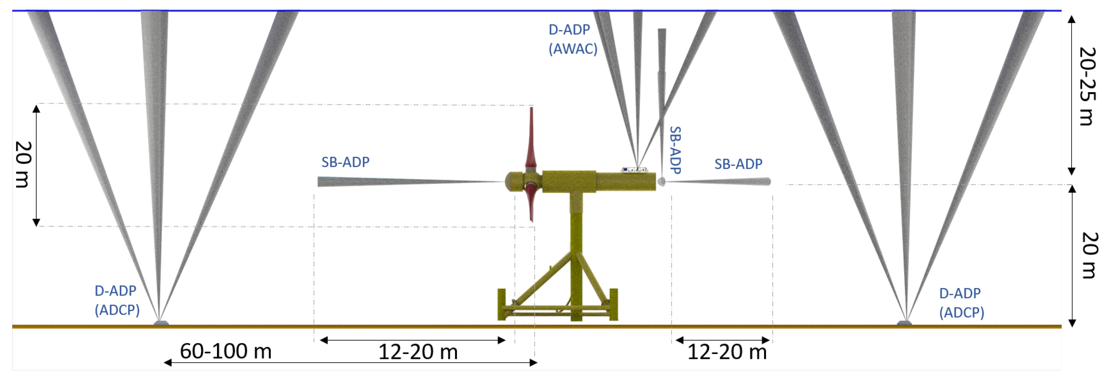
Acoustic Doppler velocimetry was the predominant measurement technique augmented with pressure sensors, echo-location of strongly acoustically reflective boundaries, data from local met-masts and information on the position, orientation and status of the proximal tidal energy converter. Table 2 lists the main instruments used, their summary specification and location of installation. Once collated and harmonised, these datasets form a database that can be queried against multiple combinations of machine and environmental conditions. This is discussed further in Section 5.1. Contemporaneous operation with the TEC was prioritised in most deployments, i.e., sensor deployment duration was prioritised over high frequency sampling. Up to twelve single-beam Doppler instruments were installed per TEC deployment. Figure 3 shows a schematic representing the range and installation position of these multiple single-beam devices and provides indicative instrument acoustic sampling ranges. Section 3.1 discusses usable profiling regions.
2.3. Summary of the Acoustic Doppler Profiling Technique
Acoustic Doppler profiler instruments, particularly those with geometrically-diverging configurations of acoustic beams, are widely used in the field measurement of offshore flow velocities due to the relative ease of configuration and installation, unobtrusive flow measurements, as well as the ability to sample throughout the water column (including the turbine rotor plane region). ADPs have been successfully used to characterise the mean flow conditions and energy flux at several sites for TEC installations [16,17,18,19,20,21].
Conventional ADPs emit acoustic signals from a number of transducers, typically two to five, installed on a single device. While a variety of beam configurations exists, in order to deduce a three-dimensional velocity measurement, these acoustic beams must be transmitted in at least three directions [22]. Using a practically-sized single instrument, the beam directions are therefore necessarily diverging, typically at an angle of 20°–30° from vertical [23]. Because the velocity measurement of each beam is calculated from the Doppler shift resulting from the scattering of sound by suspended particles in the water, the velocity component is measured in the direction of the beam itself. Spatial profiling is achieved by knowing the speed of sound in seawater and controlling the sample timing of reflected acoustic pulses. Control of the timing of the emission itself enables alternative modes of operation, namely mono-static and bi-static geometrically-converging multi-beam systems. This feature has been exploited in the recent development of field-scale Converging Acoustic Doppler Profiler (C-ADP) systems [24,25].
In energetic tidal flows, the instantaneous flow velocity is seen to vary over a wide range of time and length scales. When utilising D-ADPs for turbulence analysis, consideration of these varying scales is required [26,27]. Doppler noise is an inherent feature of the acoustic Doppler measurement technique, and correction methods have been employed in this work as described in Section 3.5.1 [28,29].
3. Quality Control and Post-Processing
Turbulence metrics including Turbulence Intensity (TI), described in Section 3.5, are sensitive to post-processing, and small differences in these metrics can affect the engineering decisions of turbine developers. This section provides an overview of (1) data exclusion steps and (2) post-processing techniques used in this analysis. Data exclusion steps are intentionally straight-forward with minimal removal of data being a specific aim since the focus here is to present assessment of the upper bound of TI at various TEC-applicable spatial averaging ranges and between instrument types. It is therefore important to avoid removal of real fluctuations from the measurements. Trials of advanced data exclusion methods are under-way, however, including outlier detection using techniques based on phase-space and the universal method along with methods based on flow acceleration (see [30,31,32]). This is discussed further in Section 6.1. Two distinct versions of the datasets required to recreate these results are publicly available, both the values used here and the unaltered raw data. Using the filters outlined below, for the eight D-ADP deployments capturing flood and ebb tides, the total percentage of data identified as bad in the range 3–40 m from the seabed (the region where further analyses are performed) was below 0.1%.
3.1. Exclusion of Data from Specific Profiling Regions
Data measurements acquired close to the acoustic emitter are adversely affected by both “ringing” and from the sensor disturbing the local flow field [33]. To mitigate ringing, “blanking distances”, where no velocity measurements are acquired, of 2.0 m and 0.4 m were used for seabed D-ADPs and turbine installed SB-ADPs respectively, as per the manufacturers’ guidance [34,35]. Whilst measurements acquired within the top ten percent of the water column are shown in the depth profile plots of Section 5, no further statistics are derived from data in this region where acoustic side-lobes can cause interference.
Table 3 lists the depths at which further characterisation is conducted.Lower than anticipated sensing ranges were achieved with the prototype SB-ADPs. Five meters to 15 m was selected as a reliable profiling range, featuring good signal strength whilst being sufficiently distant from the turbine structure [36]. Data were excluded entirely after a range of 25 m other than for wave surface tracking as described in Section 4.
3.2. Exclusion of Data Due to Low Signal Amplitude
Data were excluded if the returned signal amplitude (measured in counts) was below a minimum threshold. This is a crucial step for range-limited campaigns, for example where acoustic frequency is too high for the desired profile range. At the depths found in the Fall of Warness, Orkney (43–47 m), this was not the case for the seabed-mounted D-ADPs operating at 600 kHz, which can comfortably range to the surface. A fixed threshold of 80 and 55 counts was set for D-ADPs configured in narrow-band and broadband mode, respectively. Since signal strength remains strong to the surface, very few data points are removed through this filter at the ranges of interest. For SB-ADP instruments, whose higher acoustic frequency of 1 MHz leads to greater signal attenuation, a value of 23 counts was used, being several counts above the average sensor noise floor. This threshold effectively limits the maximum range to between 15 and 20 m depending on prevailing flow conditions. Although this filter affects the SB-ADPs outer ranges, no further analysis here is performed on data originating from these extremities.
3.3. Exclusion of Data by Outlier Detection
Prior to outlier detection, all velocities with a magnitude greater than 5 m/s were removed and linearly interpolated where their occurrence is isolated. A simple outlier detection method was applied to velocity signals based on moving window median absolute deviation [37]. The Median Absolute Deviation (MAD) is known to provide a robust measure of the variability of univariate data. An MAD routine was selected and applied to all datasets following an empirical trial on data that showed upper and lower limits, generated on a per-ensemble basis using three median absolute deviations and windows of twenty seconds in length, to perform more reliably than limits based on standard deviations around mean values. Identified outliers are replaced with the contemporaneous local upper or lower bound depending on the sign of instantaneous velocity.
3.4. Establishing a Reference Velocity
Reference velocity in the streamwise direction, , was created from instruments that can provide an upstream and thus ambient flow condition. For flood and ebb tides, these are seabed-mounted D-ADPs northwest and southeast of the TEC, respectively, as shown in Figure 1c. Varying instrument installation-depth is accounted for by reference to the fixed location of the TEC rotor extents, which also determine the particular D-ADP profile bins to be used. Velocity is averaged across this spatial range and time-averaged across sample sets of a duration of five minutes as discussed in Section 3.7.
3.5. Turbulent Flow Metrics: Turbulence Intensity
Turbulence analysis involves the analysis of fluctuations around a mean value [38,39]. Here, the turbulent quantity is velocity, u, which can be separated into mean and fluctuating components with the mean, , given by:
where N is the number of samples in a data ensemble and is an individual velocity measurement. Velocity fluctuations, , are described as the remaining parts of the turbulent flows following removal of the mean:
Whilst the average of these fluctuations is zero, the average of their square is not; hence, the root mean square (rms) can be used to provide a measure of fluctuation magnitude in a given ensemble:
Turbulence Intensity (TI), denoted here , is a metric used to quantify the magnitude of turbulence, particularly in the wind energy industry, and is now commonly used in the design of TECs. It is defined as the rms of the velocity fluctuations , divided by the mean velocity (see Equations (1) and (3)) over a given time period (see Section 3.7).
where the subscript u denotes a parameter concerning the streamwise flow direction.
Instrument Noise Correction
Turbulence intensity values are corrected for variance due to white noise () inherent in the acoustic Doppler technique. The corrected turbulence intensity in the streamwise direction, , is calculated from:
where is the variance in the stream-wise velocity component and is the variance due to white noise [18]. An value and corresponding is determined for each spatial bin of the measurement profile. Given that comparisons of values (and any other metric that is a percentage) can be ambiguous, the difference between two values is denoted by . The variance due to white noise is calculated using the method proposed by Richard et al. [28]. This involves a two-part curve fit of the power spectral density of velocity fluctuations, fitting to the slope as proposed by Kolmogorov [40] and a flat line corresponding to ‘white’ noise. In the presence of waves (particularly noting the limited frequency resolution and relatively high noise of a D-ADP), this method is not reliable. Table 4 shows the results of the analysis of a representative sample of D-ADP and SB-ADP data during periods where significant wave height m. Results are averaged over a velocity range of 1 m/s < < 3.3 m/s and for the D-ADP sampling occurs in the lower 20 m of the water column. The noise correction value used in subsequent D-ADP analysis was selected as 10.1 cm/s from the flood and ebb results, as it is the more conservative approach, i.e., it leads to smaller corrections.
3.6. Variation of Flow Characteristics with Depth
Channel flows vary vertically; thus, flow measurements throughout the water column are required. Resulting data can be reported as ensemble averaged depth profiles or fitted with a suitable model, e.g., a power-law [41,42]. Equation (6) gives the form of the power-law relationship of velocity with depth where is modelled velocity at a given depth (z), is the flow speed at a reference height given by and is an approximate empirically-calculated value normally in the range of 7–10. It should be noted that Equation (6) assumes no wind- and wave-driven surface effects or large-scale bathymetric features, which would significantly affect the depth profile. Figure 5 indicates the level of agreement between measured data and a fixed power-law model, (used here as an example), for ebb and flood tides in the presence and absence of waves. Previous empirically-derived estimates for the parameter varying on a per-velocity basis for this site are reported in [43]. It can be seen in Figure 5 that whilst there is good agreement with the power-law model for flood tides, for the ebb tides this model is not suitable due to flow retardation between mid-depth and the surface.
Subsequent analyses have used spatial averaging in the vertical direction as defined by three TEC installation types: floating, mid-depth and near-bottom, whose depths of installation and rotor extents are given in Table 3.
3.7. Removing the Mean from a Time-Varying Signal
Turbulent analyses are sensitive to both the data ensemble length (the defined stationarity period) and the method used to estimate the representative mean of a signal, particularly for complex and dynamic systems featuring underlying trends at multiple and overlapping time scales. An empirical study was conducted, as per [44,45], to ascertain a suitable stationarity period, and as with [44], a five minute period was selected. Whilst five- and ten-minute stationarity periods have become standard durations on which many TEC application analyses are conducted, the selection of this period for such complex flows is challenging and is discussed further in Section 6.1.
Common methods of defining the mean value of a complex signal include constant-value subtraction, removing a fitted linear or higher order polynomial model, high-pass filtering data to remove known oscillations and detrending via the moving average of the signal. Following previous sensitivity analyses [9], results presented here use linear detrending over the five-minute data ensembles due to the stability of the method in avoiding removal of real fluctuations from the signals whilst removing clear gradients.
4. Ocean Surface Wave Measurement in Tidal Channels
This section provides a brief overview of techniques used to characterise the local wave field contemporaneously with the tidal flows, which is essential to allow the identification and exclusion of periods influenced strongly by waves. If wave action in a tidal time series record is not sufficiently identified, subsequent quantification of turbulence intensity (upon which engineering decisions are made) will be misleading. The impact of not excluding wave-affected data is discussed in Section 5.1, and an example for a single summer deployment is summarised in Table 5.
Seabed-mounted D-ADPs (see Table 2) were not operated in a dedicated wave-measurement mode and were predominately configured for low sampling rates of 0.5–1 Hz due to programme constraints. A turbine-mounted D-ADP featuring a co-installed pressure sensor (located on ESIP-1) provided the ability to process wave time series through either the Pressure/U-velocity/V-velocity (PUV) method or Surface/U-velocity/V-velocity (SUV) method exploiting the strong backscatter from the surface via a dedicated vertically-orientated beam, a technique known as Acoustic Surface Tracking (AST) [46,47]. Due to technical limitations (now largely overcome in the latest generation of D-ADP systems), this instrument could not measure waves and currents simultaneously; thus, wave measurements were collected sporadically. This limited set, however, provides the campaigns’ benchmark wave information due to an advantageous depth of installation (mid-depth as opposed to seabed) and dedicated wave measurement hardware and software.
Recent analysis has exploited this instrument to validate multiple post-processing techniques to recover wave data from alternate instruments operating over far greater operational periods including (1) a vertically-orientated single beam ADP atop the TEC operating at 4 Hz, but with a limited spatial resolution of 0.4 m, (2) high frequency pressure gauges (2–10 Hz) installed on the turbine and (3) trial extraction of the wave field from seabed-mounted D-ADPs operating at sub-optimal sample rates. As an example, Figure 6 demonstrates the re-processing of a vertically-orientated SB-ADP to extract time series of wave elevation. Wave-current interaction can clearly be seen in the rising and falling of the wave amplitudes and periods. The benefits to flow characterisation that this reprocessing provides are discussed in Section 6. A detailed description of the wave measurement methodologies, processing techniques and corresponding datasets will be provided in the update to this article, which will present equivalent flow characterisations to those presented here, but in the presence of ocean waves.
5. Results
A data filtering process is outlined in Section 5.1 producing a sub-set of data excluding conditions where waves are present (identified through techniques outlined in Section 4). Analysis on this dataset generates results comprising depth profiles of streamwise velocity in Section 5.2 and depth profiles of turbulence intensity in Section 5.4 measured at locations producing ambient conditions upstream of the operating TEC for flood and ebb tides. The sensitivity of profile form to the sign of flow acceleration (Section 5.3) is shown along with, in Section 5.5, the effect on TI of applying noise correction techniques as introduced in Section 3.5.1. Turbulence intensities for two distinct sensor types, seabed-installed diverging-beam ADP and hub-height-mounted single-beam ADP, are compared for mid-depth flows in Section 5.7. Results are summarised in Section 5.8 across the multiple spatial averaging regimes important for TEC applications that are listed in Table 3.
5.1. Data Availability and Data Sub-Set Selection through Filtering
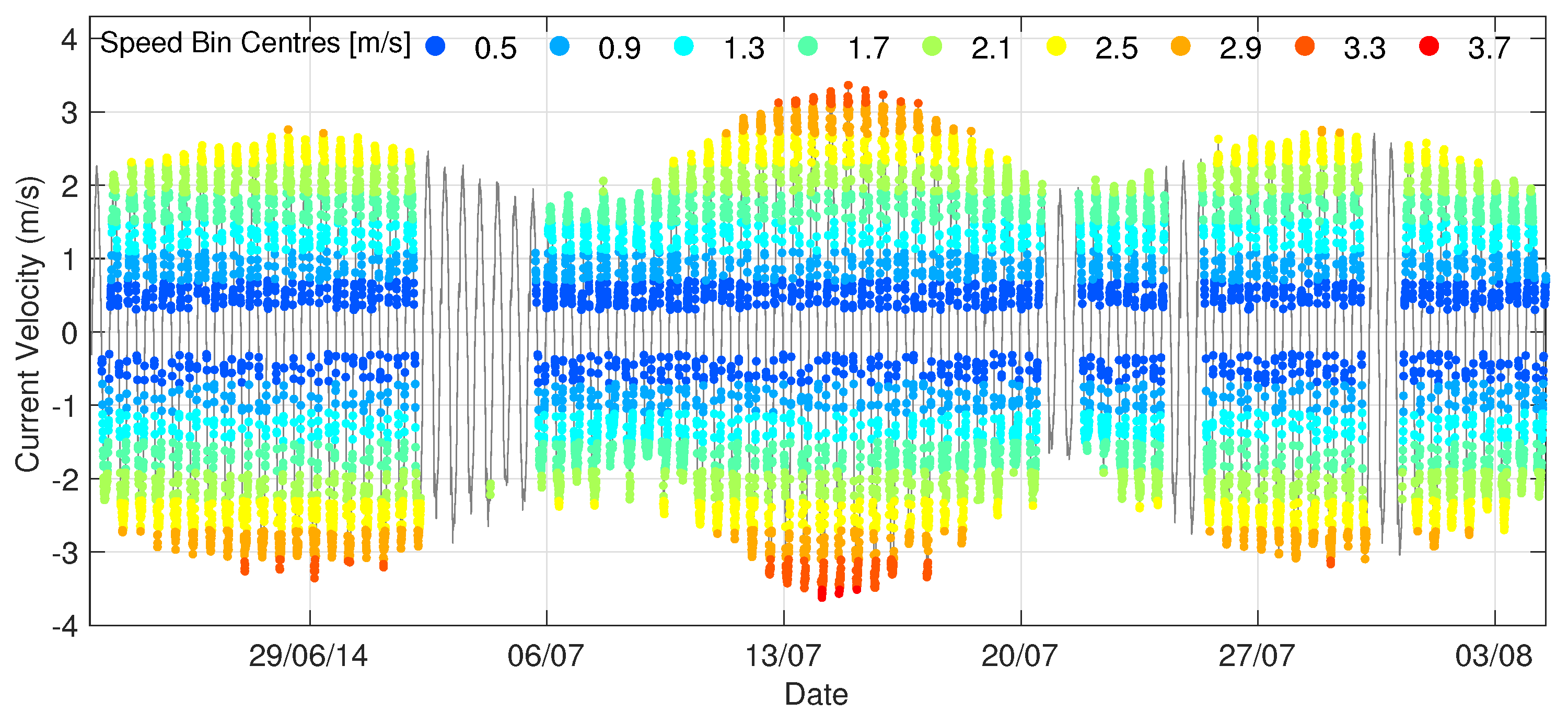
Figure 7 shows the results of a data query following the Quality Control (QC) stages outlined in Section 3. Importantly, all timestamps corresponding to site wave conditions exhibiting m have been rejected and are visible as ‘gaps’. Velocity binning of data produces coloured bands of bin width 0.4 m/s. For consistency and clarity, these coloured bands, graduated blue to red, are used in all subsequent plots relating to speed-binned data. Slack water periods, here defined as flow speeds below 0.3 m/s, have been removed. It is noted that if the analysis to derive TI included all of the data from this summer deployment, then the periods of removed wave activity would be incorporated and the wave orbital velocities would lead to high reported values of TI. For example, during a single summer campaign in 2013 of a duration of 42 days (involving instruments with ID 1 and ID 2 as per Table 1), variation in derived turbulence intensity values with and without wave filtering is shown in Table 5. In this example, the TI value applicable to floating TECs (near surface) for the unfiltered dataset is 9.2% compared to 8.4% for the wave-excluded set for ebb tide. It is notable that there is a much reduced difference when considering the flood tide, and preliminary work on the analyses of flow conditions in high wave conditions suggests sensitivity of the analyses to wave direction. Furthermore, for deployments featuring larger and more prolonged sea-states, the differences in derived TI values with and without wave exclusion filtering are considerably greater.
5.2. Depth Profiles of Streamwise Velocity
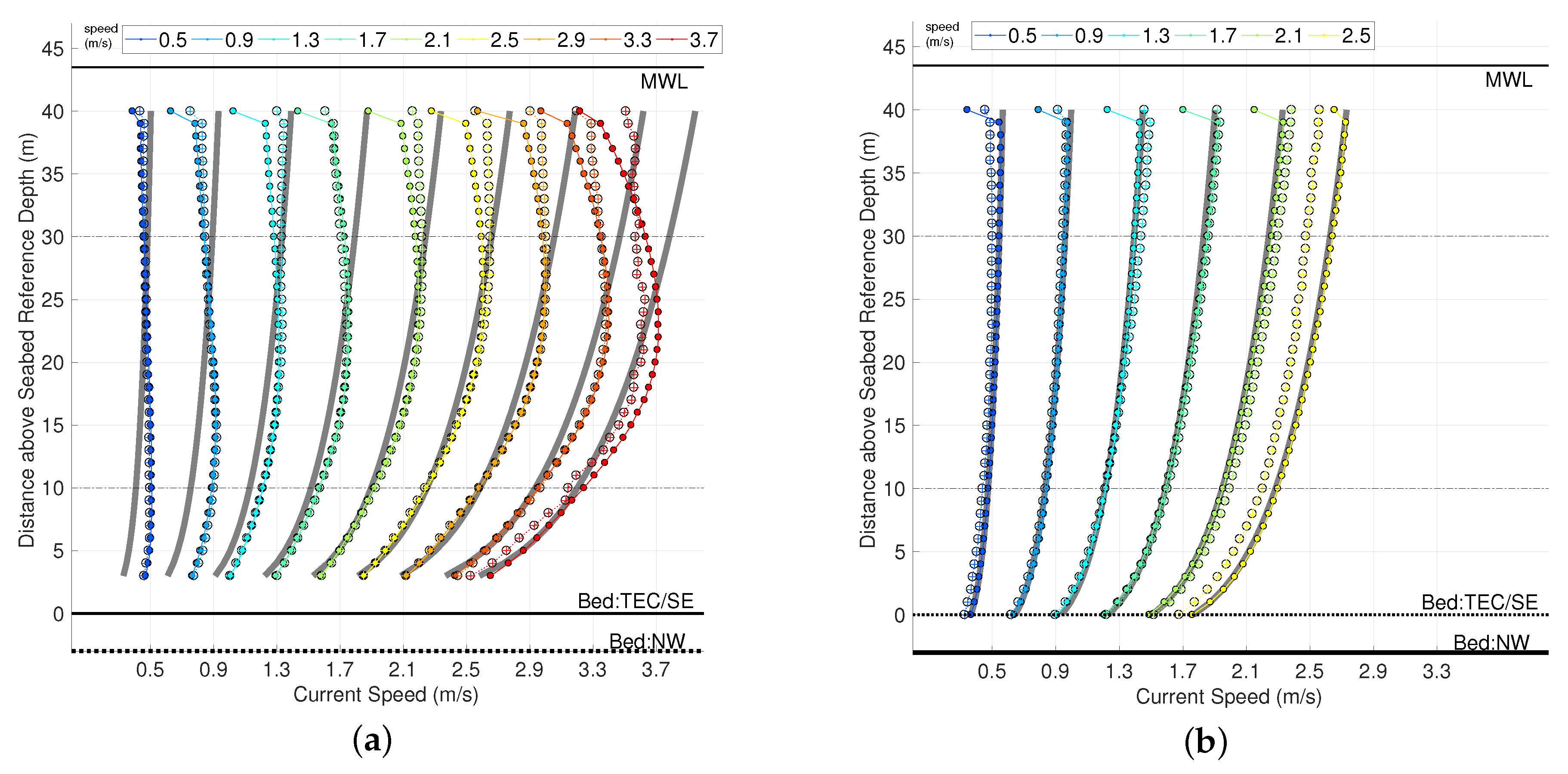
Figure 8a,b shows mean velocity depth profiles for eight separate instrument deployments for the ebb and flood tides, respectively. Averaging across the four instruments per tide is also shown as a solid line with no distinct markers. Velocity binning is carried out from 0.5 m/s to a maximum of 3.7 m/s using bin widths of 0.4 m/s. flood tides are measured by instruments located to the northwest of the TEC from deeper water with this depth indicated on these and subsequent figures as Bed: NW. Instruments measuring ebb tides (located to the southeast of the TEC) share similar depths with the TEC, which are indicated as Bed: TEC/SE. The number of returned ensembles is also shown with sample quantities ranging from a minimum of 130 to a maximum of 2032 five-minute ensembles. Flow retardation is evident from mid-depth upwards on the ebb tide. The ebb tides also display a greater degree of variability between deployments compared to the flood tide; thus, the presence of these profiles may impact the design of measurement campaigns, i.e., additional or longer deployments may be needed to capture stable long-term characterisations, which are important, for example, in energy yield calculations. This retarded or backwards-bent profile deviates from a typical power-law type fit as was previously shown in Figure 5a. On these and further plots, the extents of a 20-m rotor (typical of a 1 MW TEC) installed at approximately mid-depth are indicated by black dashed horizontal lines at 10 m and 30 m.
5.3. Depth Profiles of Streamwise Velocity Further Filtered by Flow Acceleration
Sensitivity of the profile form to tidal phase was investigated by filtering data by the sign of the flow acceleration, having taken the time-derivative of velocities after low pass filtering. Figure 9a,b shows the mean velocity depth profiles averaged over multiple D-ADP deployments. Upwards and downwards pointed chevrons represent flows that are accelerating and decelerating, respectively. Differences in the resulting profile shape are pronounced in ebb tides and minor in flood tides. Flows with average velocity of 3.3 m/s show a significant difference in the level of flow retardation between accelerating and decelerating flows. Separation of flows sharing similar average speeds across different tidal phases is discussed further in Section 6.
5.4. Depth Profiles of Turbulence Intensity
Figure 10a,b shows depth profiles of streamwise turbulence intensity derived from the same four measurement campaigns used to produce Figure 8 and Figure 9. Speed bin centres are listed in the plots. Values from individual instruments are shown as dotted lines with distinct makers, whilst the average across multiple deployments is shown as a solid marker-less line.
Since TI is calculated with velocity in the denominator, large TI values result where flow speeds are low. For TEC applications, the most relevant flow speeds are those above power-generating cut-in speed, typically > 1.5 m/s for large machines. There is significant variation in the magnitude and shape of profile between the tides. Flow retardation in the upper levels of the ebb tide impact the form of the TI depth profiles, as can be seen in Figure 10a, and across the profile, average values are lower for ebb than those for flood with the exception of the bottom 15 m.
A 1 MW TEC installed at mid-depth (with a 20-m rotor plane) would experience during ebb tides significantly higher levels of TI below the turbine centreline. At a flow speed of 3.3 m/s, the maximum range of TI between rotor top and bottom is approximately 7% varying between 7.1% (top) and 14.4% (bottom). The equivalent range for the flood tide is 9.0%–13.0%. For a floating TEC device, the magnitude and gradient of TI across the rotor plane would, for these conditions, be reduced. Summary results using varying spatial averaging dependent on envisaged TEC installation depth and rotor sizes are listed in Table 6 along with equivalent noise-corrected results (see Section 5.5).
5.5. Depth Profiles of Turbulence Intensity with Noise Correction Implemented
Instrument noise correction methods, as described in Section 3.5.1, were applied to the multiple measurement campaigns for flood and ebb tides. Results are shown in Figure 11a (ebb) and Figure 11b (flood). Corrected profiles are shown as closed circles; original data points are marked with crosses, and colours indicate velocity bins as shown in the top legend. The horizontal axis range has been reduced to emphasise TI values related to TEC operating speeds. TI profile forms are largely maintained, and expected reductions in TI can be seen, particularly in the upper half of the water column. At flow speeds above 1.9 m/s for both flood and ebb tides, spatially-averaged TI values are lowered in absolute terms by 0.8–1.0% when noise correction is applied. The effect of noise correction on TI when averaged over varying regions of the water column is detailed in Table 6.
A single average value for noise correction of 10.1 cm/s has been applied to all D-ADP instruments for both tides. Further work is required to assess the suitability of this value across the entire dataset and seasons. Investigation of the dependency or otherwise of this correction value on individual instrument configurations, as well as on environmental parameters such as flow speeds and flow turbidity is ongoing. Presently, this value is approximately 30–50% below the recommended value provided by the manufacturer. Evidence that this correction value is conservative and thus should be included in calculations of TI is provided in Section 5.7 during the comparison between differing instrument types.
5.6. Sensitivity of Turbulence Intensity to Spatial Averaging
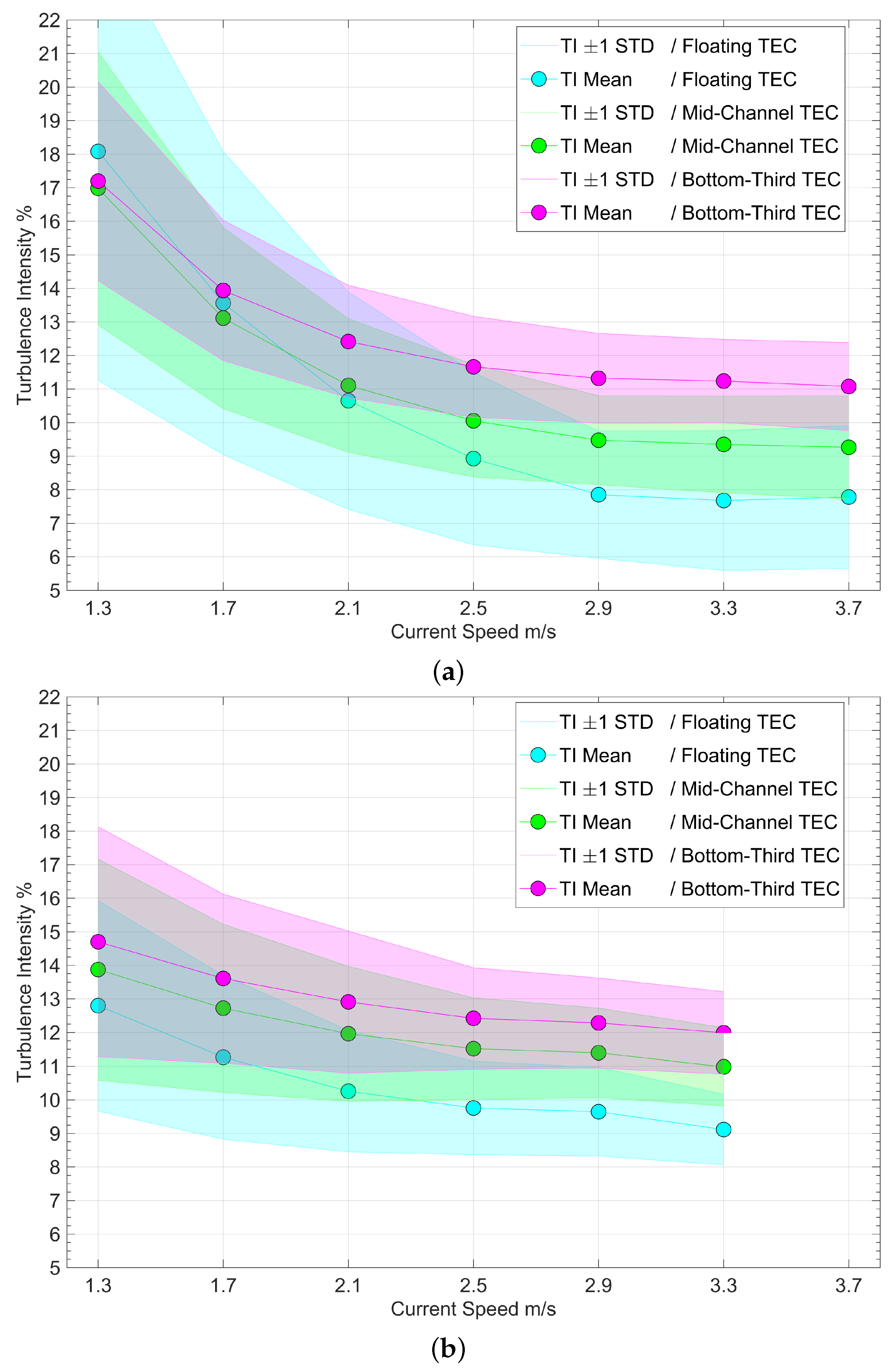
Figure 12a,b shows the dependency of TI on mean flow speed and includes the level of variation in TI across varying depths for ebb and flood tides, respectively. The magnitude of variation is indicated by the coloured shaded regions, which are plotted at one standard deviation above and below each mean value. As predicted by the higher levels of variation in ebb velocity profiles near the surface (see Figure 8a), the level of variation in TI within the sampled region applicable to a Floating TEC, indicated in Figure 12a as a cyan shaded region, is greater than the variation seen at mid-depths (green region) and lower depths (magenta region). In comparison to ebb tides, flood tides feature consistently higher TI values with smaller deviations between vertically-sampled layers.
Figure 12 makes clear the sensitivity to the specification of spatial averaging and tidal direction to any resulting characterisation of TI for this site.
5.7. Comparison of Mid-Depth Turbulence Intensity as Measured by SB-ADP and D-ADP
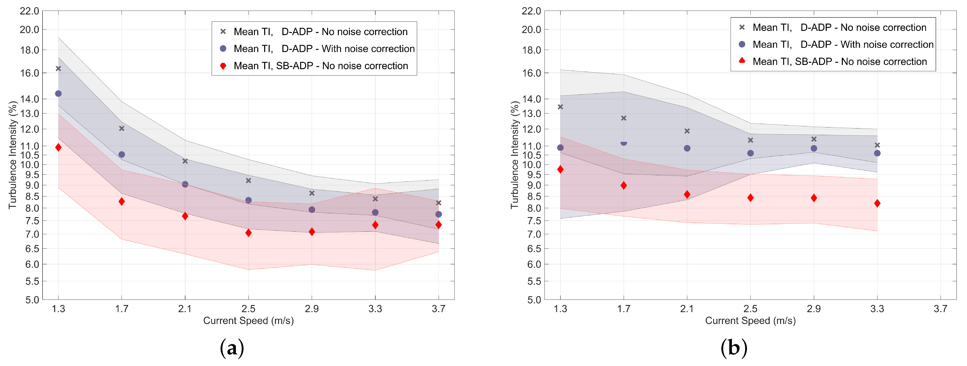
The availability of a single-beam ADP installed at mid-channel depths and operating at faster sampling rates with increased spatial resolution compared to industry standard D-ADPs (2–4 Hz/0.4 m bins compared to 0.5–1 Hz/1 m bins) enables an investigation of the level of agreement in TI values produced by these instrument types. The resulting Figure 13a,b shows the comparison of SB-ADP measurements of TI to those sampled from the equivalent depth bin using seabed-mounted D-ADPs for ebb and flood tides, respectively. A log scale is used for the Y-axis to allow improved differentiation of clustered TI values. The magnitude of the variation within each velocity bin is indicated by the shaded regions, which are plotted at one standard deviation from the instrument mean values: indicated as grey crosses and blue filled circles for D-ADP without and with noise correction, respectively, and red diamonds for SB-ADP with no noise correction applied.
The SB-ADP returns consistently and significantly lower TI values compared to the D-ADP, with a greater degree of difference compared to D-ADP values on the flood tide. At 3.3 m/s flow speed uncorrected and corrected, respectively, flood tide TI for the D-ADP is 11.0% and 10.6% compared to 8.2% for SB-ADP. Equivalent ebb tide values are 8.4%, 7.8% and 7.3%. An increase in SBD-ADP reported mean TI of approximately 0.5% (with increased variation around the mean) at flow speeds above 3.3 m/s is evident in Figure 13a. On further inspection, this is caused by periods of operation with incorrect configuration due to operator error (SB-ADPs were configured remotely and daily over many months and seven TEC deployments). Visual inspection of data shows regions featuring “velocity wrapping” whereby the sensor has been configured with too small a velocity measurement range. This manifests as incorrectly high TI values in affected ensembles. Three durations of incorrect configurations on a single instrument were manually identified and removed, totalling 9.0% of this data sub-set (234 out of 2604 five-minute ensembles), which reduced the previously large unexpected increase in TI at these flow speeds to the levels shown here.
5.8. Summary Tables: Comparative Turbulence Intensity Values
Table 6 summarises turbulence intensity results for four types of sampling range in the vertical direction with and without the implementation of noise-correction. Results have been further divided into three velocity groupings. TI derived from SB-ADP measurements are also shown.
6. Discussion
During the measurement campaigns described in Section 2, a significant volume of met-ocean data (now available publicly as outlined in Section 8) was produced by multiple instrument types operating in various configurations (as outlined in Section 2.3). These data were post-processed according to the procedures reported in Section 3 and further filtered by the results of the wave measurement and wave inference activities outlined in Section 4. The results shown have been limited to a subset of data and include analysis of streamwise depth profiles, in the absence of waves, of velocity and turbulence intensity. An investigation of the effects of the sign of flow acceleration on the resulting depth profiles is also provided. In addition, through access to SB-ADP sensors installed at mid-depth, a comparison of derived turbulence intensity in this region acquired by both SB-ADP and seabed-installed D-ADP has been carried out.
6.1. Processing and Filtering Data
Data QC has been implemented with the aim of maximising data availability for subsequent processing. Amplitude thresholds have been chosen so as to only reject data from beyond the normal operating range of each instrument, thus affecting horizontally-orientated SB-ADPs primarily. As described in Section 3.1, measurements proximal to instrument transducers and large bodies (the TEC) and the surface have not been used in subsequent analysis. A moving median deviation (MAD) filter was also applied, and in tandem with the standard scaling parameter of three and a window of 20 s, data removal was minimal. Noise correction was applied to D-ADP datasets following completion of a study (Section 3.5.1), which provided a static correction value, = 10.1 cm/s, for D-ADP instruments, and results have been reported throughout for both noise-corrected and uncorrected data. It should be noted that this correction value is approximately 30–50% smaller than that returned by the sensor manufacturer’s software prediction. The noise-correction study is currently being extended to assess sensitivity to sensor configuration, e.g., sample rate, and environmental conditions, e.g., varying flow speeds.
It was observed that for a single SB-ADP instrument during ebb tides, the level of variation in returned statistics had dramatically increased for high flow speeds. Further investigation revealed data acquired during periods of incorrect instrument configuration had passed QC. These were manually removed by generating time exclusion ranges and the results updated. Work is ongoing in developing improved data filtering routines for SB-ADPs to exclude measurements based on original sensor configurations. This is largely a task involving updating instrument meta-data and improving database homogenisation.
A trial of advanced outlier detection (see Section 3.3) is under-way with early results showing the universal method to be promising as a filter for D-ADPs of the type used in this work. The suitability of using single fixed parameters with these methods across varying instruments and environmental conditions is being assessed.
The selection of a 5-min stationarity period was taken from a pragmatic engineering viewpoint: TEC developers use numerical tools built on current site characterisation practices using 5-min averages; previous studies involving energetic tidal channels specify this duration; and a preliminary study conducted at the time of data acquisition showed that by 5 min for both tides, the rate of change of signal metrics, e.g., streamwise velocity variance, was small and stable (having undergone rapid decelerations during shorter averaging periods). Whilst this work has focused on the sensitivity of flow characterisations to tide direction, spatial averaging and instrument selection in the absence of waves, a dedicated piece of work on the stationarity of tidal flows is, however, warranted and has commenced in collaboration with the School of Mathematics. We will revisit the prescription of a suitable period over which to temporally average values from a statisticians viewpoint and conduct new sensitivity analyses.
Two distinct versions of the datasets required to recreate these results are publicly available, both the values used here and the unaltered raw data.
6.2. Streamwise Flow Velocities
Depth profiles of streamwise velocity are shown to exhibit differing forms between ebb (Figure 8a) and flood (Figure 8b) tides. Ebb tides at this location feature slower flows in the top one third of the water column compared to mid-depth flow speeds, deviating from standard models such as power-laws as discussed in Section 3.6, and show a greater degree of spatial and/or temporal variation in the depth profile form across multiple seabed instrument campaigns as shown in Figure 8a. This velocity retardation and high variability may have particular consequences for TEC developers who operate their devices nearer to the surface, using floating TECs for example. Since many industry-standard flow characterisation metrics, e.g., turbulence intensity, rely on descriptions of the underlying mean flow, careful consideration of the spatial variation with depth and measurement campaign duration is required to capture the appropriate mean flow description.
It is shown in Figure 9 that tidal accelerations should be considered during flow characterisation. Ebb tides at this site, when the sign of acceleration is included in data filtering, present differing velocity depth profiles. This would be expected to impact additional flow metrics including turbulent intensity and turbulent length scales, suggesting that reporting on a given metric against velocity alone could obfuscate important trends compared to analysis considering acceleration.
In addition, the presence of waves within data records also affects these time-averaged velocity-binned depth profiles of streamwise velocity, as seen in Figure 5. Filtering by wave regime is thus necessary when characterising mean flows. This will be expanded in a future article where analysis will include sensitivity to the varying wave conditions including wave heights, periods and directions.
6.3. Turbulence Intensities
The turbulence intensity plots shown in Figure 10 show very different levels of TI with depth between ebb and flood and furthermore illustrate that supplying a single value for TI for a tidal site is problematic and misleading. Varying the extent of included data in the vertical direction for flow perturbations and local velocity field impacts the resulting TI values as does the velocity range of interest as illustrated in Figure 12 and summarised in Table 6. Across the provided scenarios for tidal turbine installation position, TI in absolute terms varies by 1.7% for flood tides and 1.9% for ebb tides at speeds greater than 0.3 m/s. When considering only faster flows, at speeds greater than 1.9 m/s, TI is shown to vary by 2.7% for flood tides and 2.6% for ebb tides. These levels of variation are important, as they will have an impact on machine component selection and TEC device design. Whilst specifying a region of installation and rotor plane extent are important, in that rotor loading is dominated by these flows, other aspects of TEC operation including structural loading and the effects of the generated wake may require knowledge of the entire depth profile of TI.
Importantly, an inter-instrument comparison (described in Section 5.6) of mid-height turbulence intensities has been carried out. Given the advantageous location of SB-ADP, which allows direct sampling of streamwise velocity at mid-channel depths, the SB-ADP should be considered the baseline measurement for streamwise turbulence intensity characterisation. The SB-ADP method results in lower measured TI compared to D-ADP (Figure 13 and Table 6) and therefore provides us with confidence that the turbulence intensity values reported herein, for multiple spatial sampling regimes across both flood and ebb tides with the effects of waves removed, remain conservative and thus are suitable as reference values, for these flow types, for engineering applications in tidal energy.
This work has been conducted on a large dataset that has been filtered to prevent flow characterisations incorporating effects due to the presence of waves. A follow-up publication is in preparation detailing flow characterisation in the presence of varying wave conditions.
7. Conclusions
A data analysis to characterise depth varying mean velocity and Turbulence Intensity (TI) profiles at different phases of tidal flow at the Fall of Warness tidal test site within the European Marine Energy Centre (EMEC), Orkney, U.K., has been presented in this paper. These flow parameters are shown to vary considerably between flood and ebb tides. Unlike flood tides, ebb tides exhibit slower flows in the top one third of the water column compared to mid-depth flow speeds and feature, on average, lower turbulence intensities. Quantification of these parameters has been shown to exhibit significant sensitivity to: the vertical extents over which spatial averaging is conducted, the implementation of noise-correction methods on seabed installed D-ADP instruments and the magnitude of the local contemporaneous wave field, although analysis here focuses on conditions where wave-effected data have been excluded. In addition, during ebb tides in particular, whether the tide is accelerating or decelerating affects the form of the vertical velocity profile.
In terms of characterisation of mean flows, these are important factors to be considered by TEC developers, as many industry-standard flow characterisation metrics (e.g., turbulence intensity, length scale, etc.) depend on descriptions of the underlying mean flow. Careful consideration of the spatial averaging, measurement campaign duration, data processing and data filtering for the presence of surface waves is required to capture appropriate mean flow description.
In terms of the fluctuating component of the flow, turbulence intensity is shown to vary significantly between ebb and flood tides both in depth profile and spatially-averaged values. Averaged across a wide velocity range, TI is approximately 16% larger, relatively, on flood tide compared to ebb tide. TI depth-averaged over the middle 20 m of the channel at flow speeds above 1.9 m/s was found to be 11.7% for flood and 10.1% for ebb tides without noise correction and 10.9% and 9.3% with noise correction implemented. Selection of vertical averaging extents was found to strongly influence TI, which in absolute terms shows variation of 2.6% across both tides giving a maximum relative difference (when compared to the lowest value) for flood and ebb tides of 26% and 29%. These levels of variation have an impact on machine component selection, fatigue loading and TEC device design.
A novel comparison of mid-height turbulence intensities was conducted using multiple instrumentation arrays integrated with a deployed tidal turbine. Measurements made by SB-ADP reveal lower TI with relative reductions of up to 21% (depending on tide and averaging regime) compared to proximal D-ADPs. These SB-ADPs measure mid-depth flows directly at faster sampling rates with greater spatial precision and as such should be considered the baseline measurement for streamwise turbulence intensity characterisation in further analyses.
8. Availability of the Dataset
Environmental data acquired between June 2011 and October 2014 have been made available under two parallel activities: field data acquired in October 2014 are archived permanently at the Energy Data Centre of the UK Energy Research Centre (UKERC-EDC) http://data.ukedc.rl.ac.uk, whilst the latest data and re-analyses are hosted at http://redapt.eng.ed.ac.uk. This latter set contains updated information, re-analyses and field data collected beyond October 2014. Processed subsets are being transferred to the University of Edinburgh permanent digital archive where the data used within this article are already available [1,48].
Acknowledgments
This work was funded by the Engineering and Physical Sciences Research Council (EPSRC) through the Flows Waves and Turbulence (FloWTurb) Project (EPSRC EP/N021487/1). This work stems from the Reliable Data Acquisition Platform for Tidal (ReDAPT) Project funded by the Energy Technologies Institute (ETI). In addition, this work was further facilitated by the EPSRC through their institutional Impact Acceleration Accounts (IAA) via awards to the lead author, which provided critical support in maintaining the continuity of met-ocean data analysis between the two previously listed research projects. Maps were generated with bathymetry data provided by Marine Scotland.
Author Contributions
Brian G. Sellar was the lead researcher for the University of Edinburgh during the ReDAPT project, and in this role, he designed, managed and executed all aspects of the field measurement campaigns. He has also co-directed the re-analysis of data under the FloWTurb project. Gareth Wakelam has conducted re-analysis of ReDAPT data and has assisted in the preparation of this article. Duncan R. J. Sutherland assisted in the original acquisition of the ReDAPT data and in the preparation of this article. David M. Ingram developed and helped execute the ReDAPT project as University of Edinburgh Co-Investigator and provided input and internal review of this article. Venugopal Vengatesan as the Principal Investigator of the FloWTurb project co-directed this re-analysis of ReDAPT data and supported this specific article by providing internal review.
Conflicts of Interest
The authors declare no conflict of interest.
References
- Sellar, B. Metocean Data Set from the ReDAPT Tidal Project: Part 1 of 7. 2011–2014. Available online: http://dx.doi.org/10.7488/ds/1686 (accessed on 6 March 2017).
- Gunn, K.; Stock-Williams, C. Fall of Warness 3D Model Validation Report: ETI REDAPT MA1001 PM14 MD5.2; Technical Report; E.ON New Build & Technology: Coventry, UK, 2012. [Google Scholar]
- Afgan, I.; Ahmed, U.; Apsley, D.; Stallard, T.; Stansby, P. CFD Simulations of a Full-Scale Tidal Stream Turbine: Comparison Between Large-Eddy Simulations and Field Measurements: ETI REDAPT MA1001 MD1.4; Technical Report; School of MACE, University of Manchester: Manchester, UK, 2014. [Google Scholar]
- Smith, S.; Way, S.; Thomson, M. Environmental Modelling Validation ReportETI REDAPT MA1001 MD6.2; Technical Report; GL Garrad Hassan: Bristol, UK, 2014. [Google Scholar]
- Alstom Ocean Energy. ReDAPT—Initial Operation Power Curve (MC7.1); Technical Report; Alstom Ocean Energy: Nantes, France, 2014. [Google Scholar]
- Plymouth Marine Laboratory. ReDAPT—Final Report: Anti-Fouling Systems for Tidal Energy Devices (ME8.5); Technical Report; Plymouth Marine Laboratory: Plymouth, UK, 2014. [Google Scholar]
- DNV GL—Energy, Renewables Certification—Wave and Tidal. Horizontal Axis Tidal Turbines; Technical Report; DNV GL—Energy, Renewables Certification—Wave and Tidal: Høvik, Norway, 2014. [Google Scholar]
- Alstom Ocean Energy. ReDAPT—Public Domain Report: Final (MC7.3); Technical Report; Alstom Ocean Energy: Nantes, France, 2015. [Google Scholar]
- Sellar, B.; Sutherland, D. ReDAPT Tidal Site Characterisation: Final Report (MD3.8); Technical Report; University of Edinburgh: Edinburgh, UK, 2015. [Google Scholar]
- Milne, I.; Day, A.; Sharma, R.; Flay, R. The characterisation of the hydrodynamic loads on tidal turbines due to turbulence. Renew. Sustain. Energy Rev. 2016, 56, 851–864. [Google Scholar] [CrossRef] [Green Version]
- McNaughton, J.; Harper, S.; Sinclair, R.; Sellar, B. Measuring and modelling the power curve of a Commercial-Scale tidal turbine. In Proceedings of the 11th European Wave and Tidal Energy Conference (EWTEC), Nantes, France, 6–11 September 2015. [Google Scholar]
- Milne, I.; Sharma, R.; Flay, R.; Bickerton, S. The role of onset turbulence on tidal turbine blade loads. In Proceedings of the Australasian Fluid Mechanics Conference, Auckland, New Zealand, 5–9 December 2010. [Google Scholar]
- Blackmore, T.; Myers, L.E.; Bahaj, A.S. Effects of turbulence on tidal turbines: Implications to performance, blade loads, and condition monitoring. Int. J. Mar. Energy 2016, 14, 1–26. [Google Scholar] [CrossRef]
- MacEnri, J.; Reed, M.; Thiringer, T. Influence of tidal parameters on SeaGen flicker performance. Philos. Trans. R. Soc. Lond. A Math. Phys. Eng. Sci. 2013, 371, 20120247. [Google Scholar] [CrossRef] [PubMed]
- Evans, P.; Armstrong, S.; Wilson, C.; Fairley, I.; Wooldridge, C.; Masters, I. Characterisation of a Highly Energetic Tidal Energy Site with Specific Reference to Hydrodynamics and Bathymetry. In Proceedings of the 10th European Wave and Tidal Energy Conference (EWTEC), Aalborg, Denmark, 2–5 September 2013. [Google Scholar]
- Fairley, I.; Evans, P.; Wooldridge, C.; Willis, M.; Masters, I. Evaluation of tidal stream resource in a potential array area via direct measurements. Renew. Energy 2013, 57, 70–78. [Google Scholar] [CrossRef]
- Lu, Y.; Lueck, R.G. Using a Broadband ADCP in a Tidal Channel. Part I: Mean Flow and Shear. J. Atmos. Ocean. Technol. 1999, 16, 1556–1567. [Google Scholar] [CrossRef]
- Thomson, J.; Polagye, B.; Richmond, M.; Durgesh, V. Quantifying turbulence for tidal power applications. In Proceedings of the MTS/IEEE Seattle (OCEANS 2010), Seattle, WA, USA, 20–23 September 2010. [Google Scholar]
- Goddijn-Murphy, L.; Woolf, D.K.; Easton, M.C. Current Patterns in the Inner Sound (Pentland Firth) from Underway ADCP Data. J. Atmos. Ocean. Technol. 2013, 30, 96–111. [Google Scholar] [CrossRef]
- Rippeth, T.; Williams, E.; Simpson, J. Reynolds Stress and Turbulent Energy Production in a Tidal Channel. J. Phys. Oceanogr. 2002, 32, 1242–1251. [Google Scholar] [CrossRef]
- Nystrom, E.A.; Rehmann, C.R.; Oberg, K.A. Evaluation of Mean Velocity and Turbulence Measurements with ADCPs. J. Hydraul. Eng. 2007, 133, 1310–1318. [Google Scholar] [CrossRef]
- Gunawan, B.; Neary, V.S. ORNL ADCP Post-Processing Guide and MATLAB Algorithms for MHK Site Flow and Turbulence Analysis; Technical Report; Oak Ridge National Laboratory: Oak Ridge, TN, USA, 2011.
- RD Instruments. ADCP Coordinate Transformation: Formulas and Calculations; Technical Report; RD Instruments, Teledyne: Poway, CA, USA, 1998. [Google Scholar]
- Sellar, B.; Harding, S.; Richmond, M. High-resolution velocimetry in energetic tidal currents using a convergent-beam acoustic Doppler profiler. Meas. Sci. Technol. 2015, 26, 085801. [Google Scholar] [CrossRef]
- Hay, A.E.; Zedel, L.; Nylund, S.; Craig, R.; Culina, J. The Vectron. In Proceedings of the 2015 IEEE/OES Eleveth Current, Waves and Turbulence Measurement (CWTM), St. Petersburg, FL, USA, 2–6 March 2015. [Google Scholar]
- Boldt, J.A. Use of Numerical Simulations to Investigate the Performance of a Virtual Acoustic Doppler Current Profiler in Characterizing Flow. Master’s Thesis, University of Illinois, Champaign, IL, USA, 2013. [Google Scholar]
- Richmond, M.; Harding, S.; Romero-Gomez, P. Numerical performance analysis of acoustic Doppler velocity profilers in the wake of an axial-flow marine hydrokinetic turbine. Int. J. Mar. Energy 2015, 11, 50–70. [Google Scholar] [CrossRef]
- Richard, J.B.; Thomson, J.; Polagye, B.; Bard, J. Method for identification of Doppler noise levels in turbulent flow measurements dedicated to tidal energy. Int. J. Mar. Energy 2013, 3, 52–64. [Google Scholar] [CrossRef]
- Durgesh, V.; Thomson, J.; Richmond, M.C.; Polagye, B.L. Noise correction of turbulent spectra obtained from acoustic Doppler velocimeters. Flow Meas. Instrum. 2014, 37, 29–41. [Google Scholar] [CrossRef]
- Goring, D.G.; Nikora, V.I. Despiking acoustic Doppler velocimeter data. J. Hydraul. Eng. 2002, 128, 117–126. [Google Scholar] [CrossRef]
- Cea, L.; Puertas, J.; Pena, L. Velocity measurements on highly turbulent free surface flow using ADV. Exp. Fluids 2007, 42, 333–348. [Google Scholar] [CrossRef]
- Donoho, D.L.; Johnstone, J.M. Ideal spatial adaptation by wavelet shrinkage. Biometrika 1994, 81, 425–455. [Google Scholar] [CrossRef]
- Muste, M.; Kim, D.; Gonzalez-Castro, J.; Burkhardt, A.; Brownson, Z. Near-Transducer Errors in Acoustic Doppler Current Profiler Measurements. In Proceedings of the World Environmental and Water Resource Congress, Omaha, NE, USA, 21–25 May 2006. [Google Scholar]
- RD Instruments. Acoustic Doppler Current Profiler Principles of Operation A Practical Primer, 2nd ed.; RD Instruments: Poway, CA, USA, 1996. [Google Scholar]
- Nortek, A.S. Comprehensive Manual; Technical Report; Nortek: Rud, Norway, 2013. [Google Scholar]
- Sutherland, D.R.J. Assessment of Mid-Depth Arrays of Single Beam Acoustic Doppler Velocity Sensors to Characterise Tidal Energy Sites. Ph.D. Thesis, University of Edinburgh, Edinburgh, UK, 2015. [Google Scholar]
- Rousseeuw, P.J.; Croux, C. Alternatives to the Median Absolute Deviation. J. Am. Stat. Assoc. 1993, 88, 1273–1283. [Google Scholar] [CrossRef]
- Reynolds, O. On the Dynamical Theory of Incompressible Viscous Fluids and the Determination of the Criterion. Philos. Trans. R. Soc. Lond. A 1895, 186, 123–164. [Google Scholar] [CrossRef]
- Pope, S. Turbulent Flows, 1st ed.; Cambridge University Press: Cambridge, UK, 2000. [Google Scholar]
- Kolmogorov, A. A refinement of previous hypotheses concerning the local structure of turbulence in a viscous incompressible fluid at high Reynolds number. J. Fluid Mech. 1962, 13, 82–85. [Google Scholar] [CrossRef]
- Gooch, S.; Thomson, J.; Polagye, B.; Meggitt, D. Site characterization for tidal power. In Proceedings of the MTS/IEEE Biloxi—Marine Technology for Our Future: Global and Local Challenges (OCEANS 2009), Biloxi, MS, USA, 26–29 October 2009; pp. 1–10. [Google Scholar]
- Lewis, M.; Neill, S.P.; Robins, P.; Hashemi, M.R.; Ward, S. Characteristics of the velocity profile at tidal-stream energy sites. Renew. Energy 2017, 114, 258–272. [Google Scholar] [CrossRef]
- Way, S.; Thomson, M. Site Charecterisation and Design Basis Report ReDAPT MD6.1; Technical Report; GL Garrad Hassan: Bristol, UK, 2011. [Google Scholar]
- Thomson, J.; Polagye, B.; Durgesh, V.; Richmond, M.C. Measurements of turbulence at two tidal energy sites in puget sound, WA. IEEE J. Ocean. Eng. 2012, 37, 363–374. [Google Scholar] [CrossRef]
- Petrie, J.; Diplas, P.; Gutierrez, M.; Nam, S. Data evaluation for acoustic Doppler current profiler measurements obtained at fixed locations in a natural river. Water Resour. Res. 2013, 49, 1003–1016. [Google Scholar] [CrossRef]
- SonTek. SonWave-Pro: Directional Wave Data Collection; Technical Report; SonTek: San Diego, CA, USA, 2001. [Google Scholar]
- Nortek, A.S. AWAC Acoustic Wave and Current Meter User Guide, 1st ed. Document. No: n3000-126. 2005. Available online: http://www.nortek-as.com/en/support/manuals (accessed on 14 January 2012).
- Sellar, B. Metocean Data Set from the ReDAPT Tidal Project: Part 2 of 7. 2011–2014. Available online: http://dx.doi.org/10.7488/ds/1687 (accessed on 12 March 2017).
Figure 1.
Maps showing bathymetry and coastlines for (a) the Orkney Islands, Scotland, and the location of the European Marine Energy Centre (EMEC) tidal energy test site (red rectangle). In (b), the region of the test site is expanded, and the deployment location of the TEC and multiple Diverging-beam Acoustic Doppler Profilers (D-ADP) deployments are identified as a yellow circle and further detailed in (c), where range rings (grey circles) commence at a radius of 40 m from TEC and increment every 10 m. (a) The Orkney Islands; (b) the EMEC tidal test site; (c) D-ADP deployments.

Figure 2.
The DeepGen-IV 1 MW tidal turbine being deployed from Hatston Quay, Kirkwall, Orkney. Sensor platforms Edinburgh Subsea Instrument Platform 1 (ESIP-1) and ESIP-2 visible on the turbine top of the main nacelle and the left rear on the thruster housing. Turbine hub-mounted Single-Beam (SB)-ADP position indicated (HUB), but not visible at this image angle.

Figure 3.
Instrument layout on the DeepGen-IV tidal turbine. Acoustic beams are represented in grey.
Figure 3.
Instrument layout on the DeepGen-IV tidal turbine. Acoustic beams are represented in grey.

Figure 4.
Photograph of ESIP-1 showing: (1) the Converging Acoustic Doppler Profiler (C-ADP) system; (2,3) horizontally- and vertically-orientated SB-ADPs; (4) vertically-orientated D-ADP; (5) electronics’ subsea housing.
Figure 4.
Photograph of ESIP-1 showing: (1) the Converging Acoustic Doppler Profiler (C-ADP) system; (2,3) horizontally- and vertically-orientated SB-ADPs; (4) vertically-orientated D-ADP; (5) electronics’ subsea housing.

Figure 5.
Depth profiles of streamwise velocity for (a) ebb and (b) flood tide. Solid grey lines show power-law fit (). Small filled circles and large open circles with a centred cross show flows in the absence and presence of waves, respectively. Data is binned by speed as per the top horizontal legend. MWL shows mean water level. SE and NW indicate depths at southeast and northwest positions. (a) Ebb tide streamwise velocity depth profiles. (b) Flood tide streamwise velocity depth profiles.

Figure 6.
Time series (15–18 December 2014) of significant wave height, (top), and peak period, (middle), as measured above the TEC by (black line) the benchmark instrument, the AWAC D-ADP operating in “waves mode” and (red line) a vertically-orientated SB-ADP. The vertical grey line shows the starting time of an example surface tracking analysis (bottom) showing the background amplitude return signal from the SB-ADP and the corresponding detected surface (red line).

Figure 7.
Time series of velocity data (June–July 2014) acquired by an upstream D-ADP. Filtered data are shown segregated by speed bin-centres (graduated colours). The grey line shows all acquired data: gaps represent excluded data where significant wave height, , exceeds the 0.8-m threshold.
Figure 7.
Time series of velocity data (June–July 2014) acquired by an upstream D-ADP. Filtered data are shown segregated by speed bin-centres (graduated colours). The grey line shows all acquired data: gaps represent excluded data where significant wave height, , exceeds the 0.8-m threshold.

Figure 8.
Depth profiles of streamwise velocity for (a) ebb tide and (b) flood tide. Measurements from individual deployments are shown with distinct markers. Solid lines without markers present the average flow speed across instruments for a given speed bin. (a) Ebb tide streamwise velocity depth profiles. (b) Flood tide streamwise velocity depth profiles.

Figure 9.
Depth profiles of streamwise velocity for (a) ebb tide and (b) flood tide. Measurements are averages across all available instruments. Upwards-pointed chevrons show depth profiles corresponding to periods of positive flow acceleration; downwards-pointed chevrons show depth profiles corresponding to periods of negative flow acceleration. (a) Aggregate ebb tide velocity depth profiles with additional acceleration binning. (b) Aggregate flood tide velocity depth profiles with additional acceleration binning.

Figure 10.
Depth profiles of turbulence intensity for (a) ebb tide and (b) flood tide. Values, averaged over five minutes and binned by speed, from individual sensor deployments are shown with distinct markers: open circles, stars, pluses and small closed circles. Solid lines without markers present the average TI across these separate deployments for a given speed bin (shown in the top horizontal legend). (a) Ebb tide TI depth profiles. (b) Flood tide TI depth profiles.

Figure 11.
Aggregate (averaged over four instrument deployments per tide) depth profiles of TI for (a) ebb and (b) flood tides with noise correction implemented. Profiles featuring noise correction are marked by filled circles: uncorrected raw profiles are shown as crosses. (a) Aggregate ebb tide TI depth profiles. (b) Aggregate flood tide TI depth profiles.

Figure 12.
Spatially-averaged TI against current speed for (a) ebb and (b) flood tides and corresponding levels of variation (shown as ± one standard deviation (STD)) across the specific vertically-sampled region for the three TEC installation types described in Table 3. (a) Ebb tide TI variation with speed. (b) Flood tide TI variation with speed.

Figure 13.
Turbulence intensity against current speed for (a) ebb and (b) flood tides. Filled circles show mean values of TI per velocity bin derived from noise-corrected D-ADP data. Crosses show equivalent uncorrected values. Mean values of TI measured at hub-height via SB-ADP are marked with red diamonds. Shaded areas, matching mean-marker colours, represent plus and minus one standard deviation from these means. (a) Ebb Tide TI via D-ADP and SB-ADP. (b) Flood Tide TI via D-ADP and SB-ADP.


Table 1.
Turbine-proximal deployments of D-ADPs showing unique campaign ID, date deployed and duration of deployment. Locations are shown in Figure 1c. Due to a memory card error, no data were retrieved from the Deployment (Dep) 4 “NW”.
Table 1.
Turbine-proximal deployments of D-ADPs showing unique campaign ID, date deployed and duration of deployment. Locations are shown in Figure 1c. Due to a memory card error, no data were retrieved from the Deployment (Dep) 4 “NW”.
| ID | D-ADP Name | Date Deployed | Duration Days | ID | D-ADP Name | Date Deployed | Duration Days |
|---|---|---|---|---|---|---|---|
| 0 | 01_NW_Dep0 | 2013-02-21 | 24 | 4 | 02_NW_Dep4 | 2014-04-09 | 0 |
| 1 | 01_NW_Dep1 | 2013-06-05 | 42 | 4 | 02_SE_Dep4 | 2014-04-09 | 58 |
| 1 | 02_SE_Dep1 | 2013-06-05 | 42 | 5a | 03_SE_Dep1 | 2014-06-20 | 46 |
| 2 | 01_NW_Dep2 | 2013-07-18 | 15 | 5a | 01_NW_Dep5 | 2014-06-22 | 41 |
| 2 | 02_SE_Dep2 | 2013-07-18 | 15 | 5b | 02_NW_Dep5 | 2014-07-07 | 40 |
| 3 | 01_NW_Dep3 | 2013-10-15 | 42 | 6a | TD7_01_Dep1 | 2014-09-17 | 85 |
| 3 | 02_SE_Dep3 | 2013-10-15 | 40 | 6b | TD7_02_Dep1 | 2014-09-17 | 71 |
Table 2.
Acoustic instrument summary specification.
| Instrument Name (Manufacturer) | Acoustic Frequency (kHz) | Type | Sample Rate (Hz) | Quantity | Location |
|---|---|---|---|---|---|
| ADCP (RDI) | 600 | D-ADP | 0.5–2 | 2 | Seabed near-TEC |
| AWAC (Nortek) | 1000 | D-ADP | 1 | 1 | Turbine ESIP-1 |
| AD2CP (Nortek) | 1000 | SB-ADP | 1–4 | 16 | Turbine ESIP-1&2 |
| Continental (Nortek) | 192 | SB-ADP | 1 | 1 | Turbine ESIP-2 |
| AD2CP (Nortek) | 1000 | SB-ADP | 1–4 | 1 | Turbine Hub Centreline |
Table 3.
Spatial averaging regions in the vertical direction for three TEC installation types and a narrow mid-depth sampling regime. Distances are relative to the seabed.
Table 3.
Spatial averaging regions in the vertical direction for three TEC installation types and a narrow mid-depth sampling regime. Distances are relative to the seabed.
| Turbine Installation Type | Range from Seabed (m) | Rotor Diameter (m) |
|---|---|---|
| TEC Floating | 20–38 | 18 |
| TEC Mid-Depth | 10–30 | 20 |
| TEC Deep (Bottom Third) | 9–21 | 12 |
| Channel Mid-Depth | 19–21 | N/A |
Table 4.
Correction factors reported as the standard deviation in cm/s due to sensor noise for turbine-mounted SB-ADP and seabed-mounted D-ADP data in the absence of waves.
Table 4.
Correction factors reported as the standard deviation in cm/s due to sensor noise for turbine-mounted SB-ADP and seabed-mounted D-ADP data in the absence of waves.
| Sensor | Direction | Flood (cm/s) | Ebb (cm/s) |
|---|---|---|---|
| SB-ADP | U | 6.2 | 6.2 |
| D-ADP | U | 10.1 | 10.3 |
Table 5.
Streamwise Turbulence Intensity (TI) values with and without data exclusion based on contemporaneous wave measurement for a single summer D-ADP deployment. TI is a relative percentage difference.
Table 5.
Streamwise Turbulence Intensity (TI) values with and without data exclusion based on contemporaneous wave measurement for a single summer D-ADP deployment. TI is a relative percentage difference.
| Ebb Tide | Flood Tide | |||||
|---|---|---|---|---|---|---|
| All Data | TI | All Data | TI | |||
| Floating TEC | 8.4 | 9.2 | 9.0 | 9.7 | 9.8 | 1.2 |
| Mid-Depth | 9.4 | 9.6 | 2.5 | 11.4 | 11.4 | 0.3 |
Table 6.
TI with and without noise correction for differing TEC deployment depths. Std is the standard deviation derived spatially across the vertical range.
Table 6.
TI with and without noise correction for differing TEC deployment depths. Std is the standard deviation derived spatially across the vertical range.
| Turbine Installation Type | Noise Correction | TI (%) at Three Flow Speed Ranges (m/s) | |||||
|---|---|---|---|---|---|---|---|
| 0.3 < U < 3.9 | 1.1 < U < 3.9 | 1.9 < U < 3.9 | |||||
| Mean Std | Mean Std | Mean Std | |||||
| D-ADP ebb tide | |||||||
| Floating | No | 14.4 | 11.3 | 10.7 | 5.4 | 9.1 | 4.0 |
| Floating | Yes | 12.8 | 10.1 | 9.4 | 5.3 | 8.1 | 4.1 |
| Mid-Depth | No | 14.7 | 9.4 | 11.3 | 2.9 | 10.1 | 1.5 |
| Mid-Depth | Yes | 12.9 | 7.7 | 10.3 | 2.7 | 9.3 | 1.5 |
| Deep (Bottom Third) | No | 15.6 | 8.3 | 12.7 | 2.3 | 11.7 | 1.3 |
| Deep (Bottom Third) | Yes | 13.9 | 6.5 | 11.7 | 2.1 | 11.0 | 1.3 |
| Channel Mid-Depth | No | 13.7 | 9.8 | 10.3 | 3.2 | 9.0 | 1.5 |
| Channel Mid-Depth | Yes | 12.0 | 8.2 | 9.2 | 3.0 | 8.1 | 1.6 |
| D-ADP flood tide | |||||||
| Floating | No | 15.4 | 9.4 | 10.8 | 2.1 | 10.0 | 1.3 |
| Floating | Yes | 12.5 | 7.8 | 9.5 | 2.2 | 9.1 | 1.4 |
| Mid-Depth | No | 16.7 | 9.0 | 12.4 | 2.1 | 11.7 | 1.3 |
| Mid-Depth | Yes | 13.7 | 7.2 | 11.1 | 2.2 | 10.9 | 1.4 |
| Deep (Bottom Third) | No | 17.5 | 9.1 | 13.3 | 2.2 | 12.6 | 1.5 |
| Deep (Bottom Third) | Yes | 14.5 | 7.3 | 12.0 | 2.3 | 11.8 | 1.6 |
| Channel Mid-Depth | No | 16.4 | 9.0 | 12.2 | 2.8 | 11.5 | 1.8 |
| Channel Mid-Depth | Yes | 13.5 | 7.4 | 11.0 | 2.9 | 10.7 | 1.9 |
| SB-ADP ebb tide | |||||||
| Channel Mid-Depth | No | 10.8 | 6.1 | 7.9 | 1.9 | 7.3 | 1.3 |
| SB-ADP flood tide | |||||||
| Channel Mid-Depth | No | 11.9 | 6.3 | 8.8 | 1.4 | 8.5 | 1.1 |
© 2018 by the authors. Licensee MDPI, Basel, Switzerland. This article is an open access article distributed under the terms and conditions of the Creative Commons Attribution (CC BY) license (http://creativecommons.org/licenses/by/4.0/).
Share and Cite
MDPI and ACS Style
Sellar, B.G.; Wakelam, G.; Sutherland, D.R.J.; Ingram, D.M.; Venugopal, V. Characterisation of Tidal Flows at the European Marine Energy Centre in the Absence of Ocean Waves. Energies 2018, 11, 176. https://doi.org/10.3390/en11010176
AMA Style
Sellar BG, Wakelam G, Sutherland DRJ, Ingram DM, Venugopal V. Characterisation of Tidal Flows at the European Marine Energy Centre in the Absence of Ocean Waves. Energies. 2018; 11(1):176. https://doi.org/10.3390/en11010176
Chicago/Turabian StyleSellar, Brian G., Gareth Wakelam, Duncan R. J. Sutherland, David M. Ingram, and Vengatesan Venugopal. 2018. "Characterisation of Tidal Flows at the European Marine Energy Centre in the Absence of Ocean Waves" Energies 11, no. 1: 176. https://doi.org/10.3390/en11010176
Note that from the first issue of 2016, this journal uses article numbers instead of page numbers. See further details here.