
Experimental and Numerical Investigation of Forced Convection in a Double Skin Façade

1
Department of Architecture, Niğde Ömer Halisdemir University, Niğde 51240, Turkey
2
Department of Architecture, İzmir Institute of Technology, İzmir 35430, Turkey
3
Department of Mechanical Engineering, Dokuz Eylül University, İzmir 35397, Turkey
*
Author to whom correspondence should be addressed.
Energies 2017, 10(9), 1364; https://doi.org/10.3390/en10091364
Submission received: 7 July 2017
/
Revised: 25 August 2017
/
Accepted: 5 September 2017
/
Published: 8 September 2017
(This article belongs to the Section I: Energy Fundamentals and Conversion)
Abstract
:Flow and heat transfer of the air cavity between two glass façades designed in the box window type of double skin façade (DSF) was evaluated in a test room which was set up for measurements in the laboratory environment and analyzed under different working conditions by using a computational fluid dynamics tool. Using data from the experimental studies, the verification of the numerical studies was conducted and the air flow and heat transfer in the cavity between the two glass façades were examined numerically in detail. The depth to height of the cavity, the aspect ratio, was changed between 0.10 and 0.16, and was studied for three different flow velocities. Reynolds and average Nusselt numbers ranging from 28,000 to 56,500 and 134 to 272, respectively, were calculated and a non-dimensional correlation between Reynolds and Nusselt numbers was constructed to evaluate the heat transfer from the cavity (except inlet and outlet sections) air to the inside environment and it could be used the box window type of DSF applications having relatively short cavities.
1. Introduction
A double skin façade (DSF) acting as a second building envelope usually consists of an external glazed skin and an internal skin which is made of glazed or partially glazed material. These skins are separated from each other by an air cavity. The width of this air cavity can vary from 0.2 m to more than 2.0 m. This cavity behaves like a thermal buffer zone and it can be ventilated by stack and wind effects or by using mechanical system. DSF systems are generally proposed to decrease heating loads in winter through increasing outside temperature of the internal façade using solar radiation, and to decrease cooling loads in summer by lowering the internal façade temperature due to ventilation in the cavity.
Experimental approaches under laboratory conditions provide reliable information regarding airflow, temperature distribution and heat transfer in DSF. However, it is not an easy task and the results are highly dependent on the procedure and the accuracy of the measurements. Experimental studies which were conducted under such laboratory conditions of double skin façades are presented in the literature [1,2,3,4,5]. The experimental setup in the laboratory environment allowed to obtain more reliable and a wider range of data in these studies.
In some studies, different behaviors of the forced flow in the cavity were examined experimentally and numerically by computer methods. In this regard, various computational fluid dynamics (CFD) models were developed to study the behavior of DSF or to optimize its performance. Different ventilations strategies with DSF’s inlet conditions were investigated by using CFD tools for obtaining velocity and temperature fields for reducing energy usages [6]. A CFD tool was used to predict the effect of the different venetian blind positions. The CFD study was validated with experimental results of DSF cavity which was mechanically ventilated [7]. Venetian blind positions and their thermophysical properties were also studied by CFD simulation [8,9]. Additionally, the effect of the air flow rate as an inlet condition of DSF was investigated. A CFD tool was also used for determining the energy saving of an existing building [10,11].
Different from these CFD studies, this study focuses on the investigation of the flow and heat transfer inside the individual cavity for obtaining the non-dimensional heat transfer characteristics. For that purpose, the cavity part of the experimental setup was modelled by CFD software and the experimental results were compared with the numerical results and a validity check was made for the numerical results. Then parametrical studies conducted by CFD software were evaluated by non-dimensional heat transfer characteristics for forced convection through the surfaces of DSF’s cavity. This kind of fluid flow and heat transfer problems between two parallel plates are widely studied in the literature [12,13]. The current study stands out by using different boundary conditions and the specific geometric features as a DSF cavity. The first results obtained from the experimental setup were given for the situation of natural convection condition in an enclosed cavity of the DSF [14].
The experimental setup was reorganized for forced flow condition by using the air cavity designed in the box window type of DSF. The ranges of cavity aspect ratio (width/height) of DSF and the Reynolds numbers of the air flow in the cavity of 0.10–0.16 and 28,000–56,500, respectively, are the first limitations of the current study. The solar radiation is not considered in the simulations. Instead, the corresponding temperature values measured experimentally are directly defined on the side walls of the cavity as a function of vertical position for the CFD studies. And the last limitation; the box window type of DSF are studied numerically under turbulent and forced flow conditions between two glass façades to evaluate flow and heat transfer characteristics.
2. Experimental Study
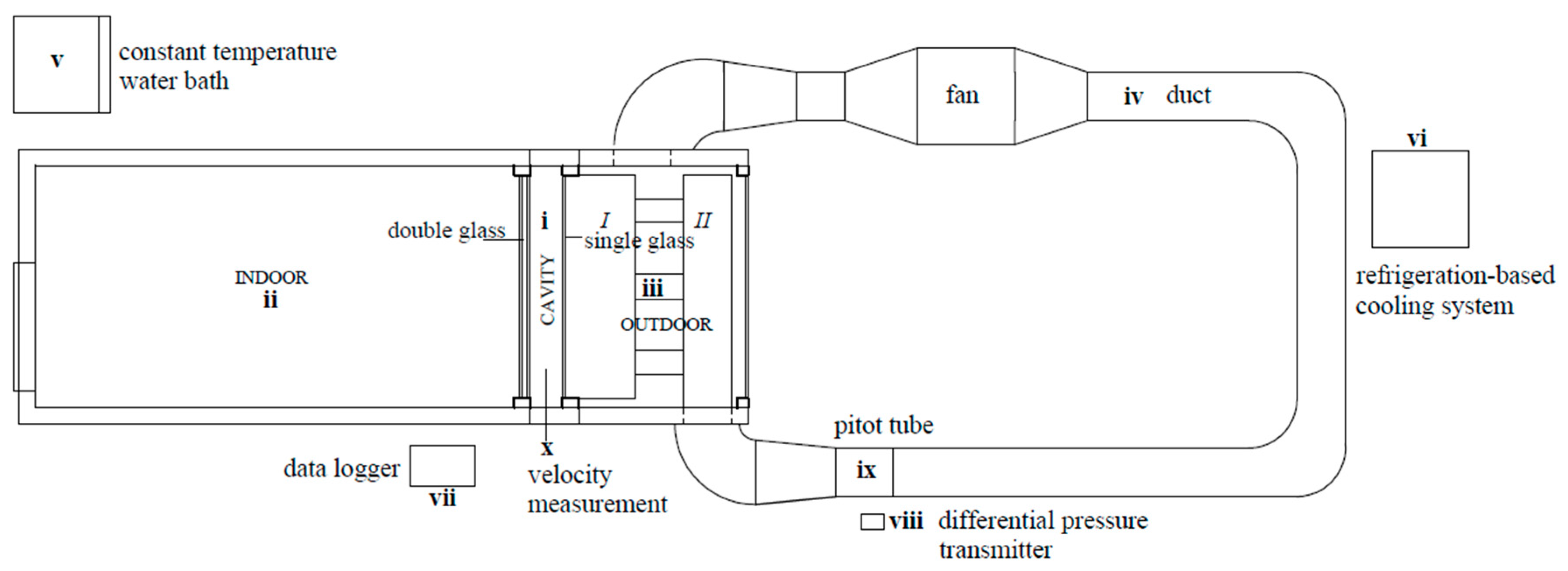
The experimental setup shown in Figure 1 is located in the Faculty of Architecture, İzmir Institute of Technology, Turkey. Flow and heat transfer was analyzed through the DSF’ cavity (i) positioned between the indoor (ii) and outdoor (iii) conditioned environments. A duct system (iv) was integrated into the system to create forced flow inside of the cavity. The indoor environment was conditioned by a constant temperature water bath v; and a refrigeration-based system (vi) cooled down the outdoor environment. Indoor and outdoor temperatures were maintained at the desired temperatures by two thermostats individually. The lengths of the indoor and outdoor environments are 3.0 m and 0.9 m, respectively. The inside dimensions of these environments are in 1.5 m (width) and 3.0 m (height). 10 cm-thick polyurethane insulation covered with metal sheets was used for the walls of the experimental environments. The cavity was designed to simulate the DSF; one of the walls was double-glazed with dimensions of 4-12-4 mm which separated from the indoor environment; the other surface was single-glazed with dimension of 4 mm which separated from the outdoor environment of the experimental setup. There were two openings for air inlet and outlet in the single-glazed exterior glass and inlet/outlet spans lied along the width of the cavity at the height of 0.2 m.
All of the measurements were recorded with a data logger indicated by (vii) in Figure 1. Air velocity in the duct was measured by using a differential pressure transmitter (DPT 2500-R8, HK Instruments, Muurame, Finland) which operated in the range of 0–100 Pa (mentioned as (viii) in Figure 1). This velocity pressure measurement obtained by a Pitot tube apparatus shown as (ix) in Figure 1 was recorded as voltage in the data logger and converted to the velocity by Bernoulli principle. Air velocity in the cavity was measured by a HD 4V3T S1 device (Delta Ohm, Padova, Italy) which was placed between the double façades linked to the data logger mentioned as (x) in Figure 1. For that purpose, the position of the prop was controlled manually from the outside of the cavity by using a fixed scale.
The duct system (iv) was integrated into the cavity at the bottom with two distribution hoods mentioned as I and II in Figure 1. The hood numbered II was fixed. The other hood (I) was mounted on the air inlet opening of the cavity and moved with the outside façade mentioned single glass of the cavity. Three flexible channels were used between these two hoods to compensate the motion. A perforated plate at the entry to the cavity was installed to create uniform flow. Fan sucked air from the air outlet of the cavity freely through an opening at the bottom of the outdoor environment (iii) which is connected to the duct cycle (iv).
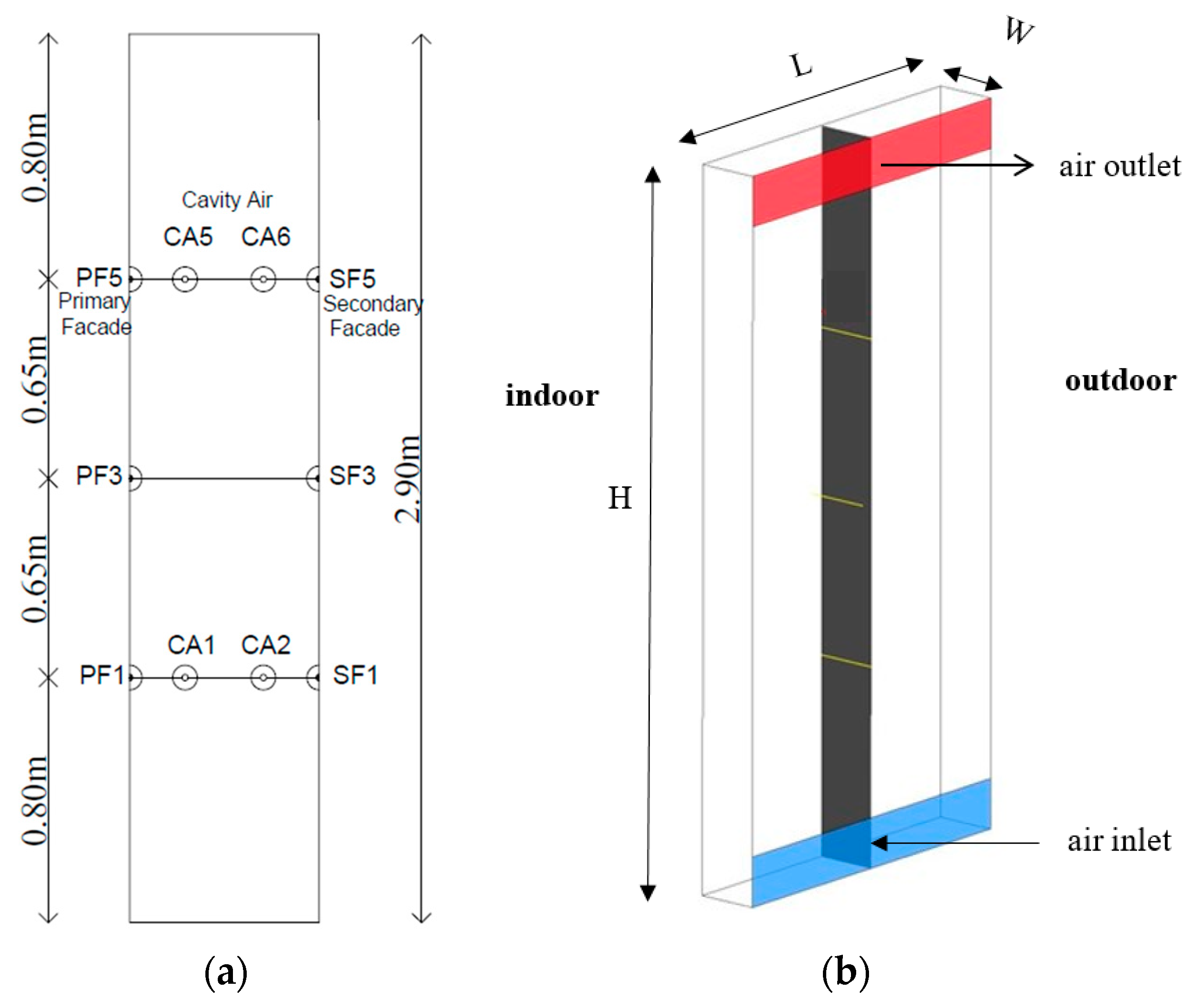
Eight T-type thermocouples coded as CA1 to 8 (CA3,4 and CA7,8 were positioned in the cavity at the same levels and the projection of the other four thermocouples) were placed inside the cavity to measure air temperature in Figure 2a. Two groups of six-T-type thermocouples (PF1-6 and SF1-6 in Figure 2a) were also connected to two inner surfaces of the cavity to measure surface temperatures (PF and SF2,4,6 were also positioned at the projection of the other six thermocouples). Cavity outer surfaces were also measured with two thermocouples at the level of 1.45 m. Air inlet temperature to the cavity was measured at the flexible channels between two hoods. Inside and outside environments were also measured.
The height and width of the cavity (i) geometry were, respectively, H = 2.9 m and L = 1.4 m (Figure 2b). Aluminum profiles, 5 cm thick were used for both façades in order to increase the durability of the glass. The depth of the cavity (i) was studied for three different situations as W = 25.0 cm, 32.5 cm and 40.0 cm. In order to adjust the depth of the cavity, limitless-geared mechanisms which were triggered by electric motors from bottom and top were used to achieve the desired span.
Calibration and Uncertainty
All thermocouples were calibrated in the calibration laboratories of İzmir Chamber of Mechanical Engineers. The calibration of the thermocouples was performed by using a PT 100 probe connected to an HP 3458 multimeter (Hewlett Packard, Palo Alto, CA, USA), both of which were calibrated in the National Metrology Institute of Turkey. The total uncertainty of the calibrated thermocouples and the data logger used in the experiments were estimated to be ±0.034 °C [15]. The depth of the cavity was checked by measuring from the points which are close to the four corners of the cavity and the middle point of the cavity and for each situation, the maximum value of deviation was detected as ±2 mm.
Differential pressure measurement system was self-calibrated. The uncertainty in relation to the differential pressure meter for the velocity measurement was defined as ±15‰ + 1 Pa. This velocity system was already calibrated by the manufacturer and the measurement values were also recorded as voltage in the data logger (vii) and converted to the velocity. The measurement accuracy of the device was defined as ±(0.2 m/s + 3% f.s.) [15]. The uncertainty of the energy transfer rate for the cavity air was calculated by considering the measurement devices and the thermophysical properties as 5.4% [16].
3. Experimental Results
The experimental conditions of the various experiments carried out are listed in Table 1. All experimental measurements reflect the average of long term measurements which were taken after the system reached the thermal equilibrium. Flow rate was controlled by driving fan rotation number for three different average rates, namely 1300, 1800 and 2300 m3/h, which were symbolized as low, medium and high flow rates, respectively. Tinlet defines the air inlet temperature, while Vinlet shows average air inlet velocity to the cavity. Thermocouples are numbered in Table 1 from T1,2avg (the average of the two thermocouple at the 0.80 m level) to T5,6avg (the average of the two thermocouples at the 2.10 m level) for PF for the portion of the primary façade facing the cavity and from T1,2avg to T5,6avg for the portion of the SF facing the cavity.
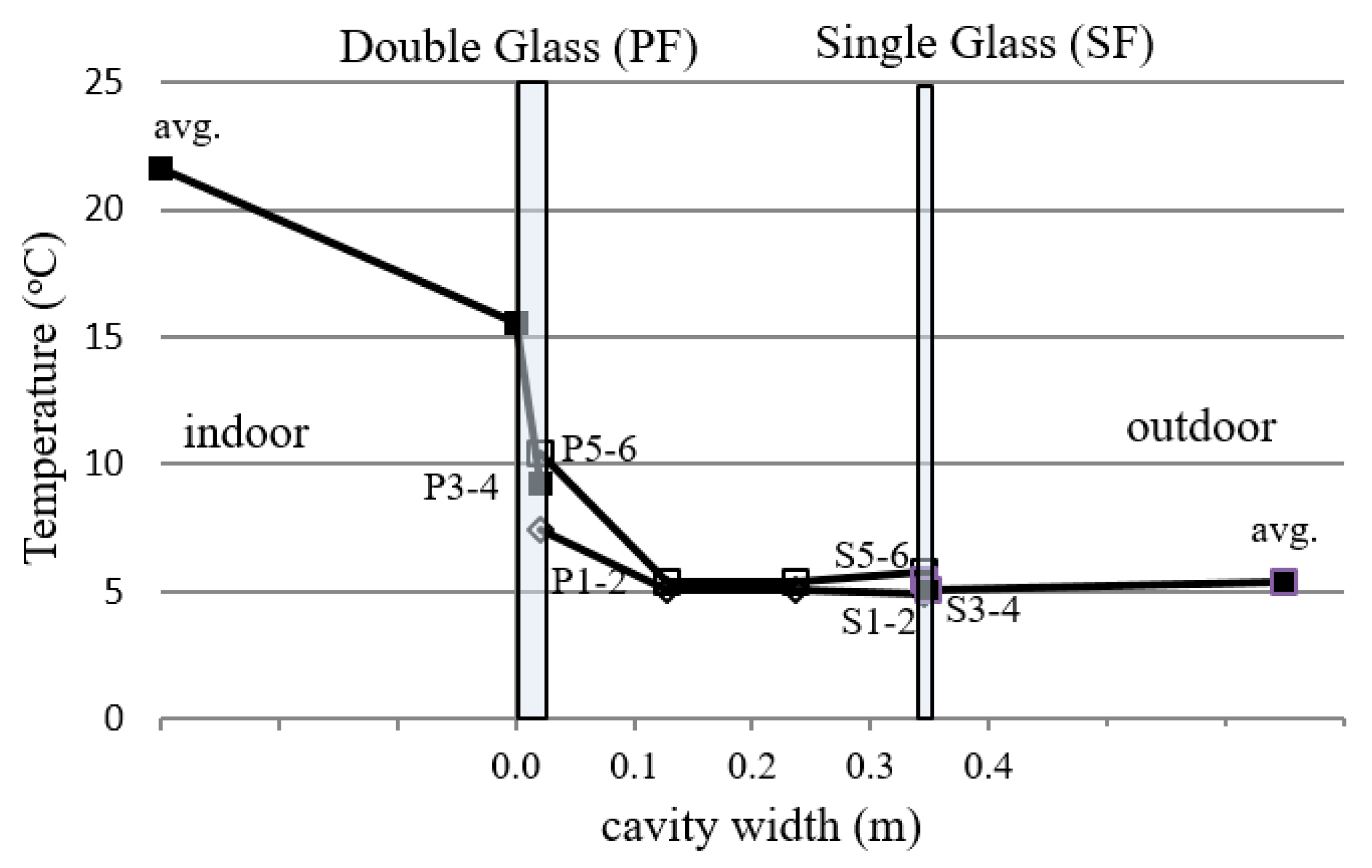
Under steady-state condition for each experiment, the temperature distribution of the system was also obtained graphically based on the values given in Table 1. The experimental study numbered 4 for low flow rate is shown in Figure 3 for 32.5 cm cavity depth. While the average temperature of the indoor environment was 21.65 °C (calculated by three thermocouples), the average temperature of the outdoor environment was 5.37 °C (calculated by two thermocouples) at the Experiment 4. Relatively low thermal resistance of the single glass (SF) did not create significant temperature drop. Due to the heat transfer which was from the indoor environment to the cavity, temperatures along the cavity and in its air flow increased on both of the surfaces. This increase was more visible on the primary façade (Figure 3).
4. Numerical Study
Under these different working conditions, the velocity, pressure and temperature changes in the cavity were examined numerically in detail.
4.1. Governing Equations
The governing equations for the Cartesian coordinate system in the following forms were used, respectively:
Mass equation,
x-momentum equation,
y-momentum equation
z-momentum equation
Energy equation,
where velocity, pressure and temperature were defined as time-averaged. Turbulence was determined for each node in the domain in terms of the local turbulence kinetic energy (k) and the diffusion rate (ε):
Large eddy simulation (LES) has been used in many studies to analyze turbulent flows in simple geometries and boundary conditions [17,18,19,20]. Although this method gives more accuracy solution, it needs more computer memories than standard k-epsilon method. In this study, k-epsilon method was used as turbulence model.
To resolve the turbulence energy and diffusion rate terms, the realizable k-epsilon turbulent model was used. In comparison to the classical k-epsilon method, the realizable model is more successful and accurate for the problems with flow separation, re-attachment and complicated secondary flows [21]. In the realizable k-epsilon method, the following additional equations are resolved to evaluate the kinetic energy and the dissipation rate, respectively:
The details of the terms and constants given in the governing equations can be found in the theory book of ANSYS [17].
4.2. Numerical Method
Calculations were conducted in the ANSYS-FLUENT version 16.0 environment based on the approach of the control volumes by forming the three dimensional numerical model of the geometry in the ANSYS environment [21]. The numerical solution is based on the following assumptions and approaches.
- The flow is steady, fully turbulent and three dimensional,
- The realizable k-epsilon turbulent model was used,
- SIMPLE algorithm was applied in the solution of the governing equations,
- Standard method was used for the separation of the pressure term,
- Second Order Upwind separation scheme was applied for the other transport equations
The SIMPLE algorithm of Patankar [22] was used to solve the pressure-velocity coupling. In the decomposition of the pressure term, the PRESTO method was used, whereas for the other transport equations, the QUICK scheme was applied [23]. In the analyses, for the all of the transport parameters, the convergence criterion was defined as 10−7.
The grid independent test for the physical model performed to determine the most suitable size of the mesh faces. There were 2,473,800 hexahedra type mesh elements in the model. While the minimum mesh volume was 1.3056 × 10⁻⁸ m3, the maximum mesh volume was 1.6465 × 10⁻⁶ m3. The total air volume was 1.0150 m3 for the cavity model. In order to analyze the changes which occurred where the air entrance and exit vents were located more precisely, the number of meshes in these zones were increased. It was observed that the convergence criterion was approximately at 10−5 levels in all of the conducted analyses.
4.3. Geometrical Setup and Boundary Conditions
The cavity geometry used for the numerical study is given in Figure 2b. The air flow in the cavity between primary (PF) and secondary façade (SF) is modeled and the results are shown along the longitudinal plane mentioned dark color. Three horizontal lines drawn in the dark color plane are shown temperature measurement sections.
Temperatures of the PF and SF surfaces (Table 1) were measured experimentally and defined as the boundary conditions of the numerical study. The other four surfaces of the rectangular cavity are assumed to be adiabatic. Air inlet and outlet sections given in Figure 2b are in the SF surface. Air inlet average velocity was taken as uniform and temperature values were also measured and used as given in Table 1. Air outlet was defined as the atmospheric pressure as a boundary condition in the ANSYS-FLUENT environment.
5. Results and Discussions
The numerical studies were conducted using the parameters in Table 1. The velocity and temperature values acquired from the experimental measurements with the numerical results are compared. Then, the distributions of air velocity, temperature and pressure in the cavity are examined and the streamlines for different working conditions are plotted. And later, the dimensionless heat transfer coefficients estimated from these results will be discussed.
5.1. Velocity Changes at the Horizontal Lines in the Middle of the Cavity
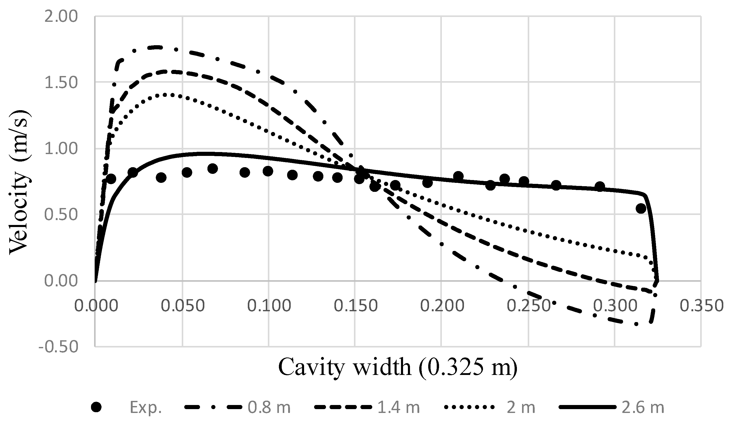
Velocity changes at various lengths on the longitudinal section were compared with the velocity values at 2.60 m height of the cavity which were measured experimentally (Figure 4). Because of the inlet flow condition of the cavity, the velocity values increased coming closer to the PF surface (0.0 m in Figure 4), when the velocity values decreased coming closer to the SF surface (0.325 m in Figure 4). The reverse flows were observed at 0.80 and 1.40 m heights of the cavity in the simulation results. Also it was seen that in the experimental results, at 2.60 m height of the cavity, the measurements which were taken along the cavity depth were coherent with the simulation results.
Forced flow oriented through the cavity height right after the cavity entrance provided that the air was lifted mostly by primary façade with the effect of the 90° turn here and created reverse flows at the secondary façade side. As the flow continued above to its situation of fully developed flow, it was affected by the section of the cavity exit. In the turbulent flow, fully developed flow hydrodynamically and thermally begins after entrance length and it is approximately taken to be 10 times of the hydraulic diameter defined as the cross sectional area and the perimeter of the cavity. Hydraulic diameters in the experiments are changed from 0.424 m to 0.622 m and the cavity height is only 2.9 m which is shorter than ten times of hydraulic diameters. Therefore, in all of the studies which were conducted here, the experimental and numerical analyses of the flow conditions mainly in the entrance region were conducted [15]. The entry length is much shorter if it is used a smaller hydraulic diameter and the effect of the reverse flows in the cavity become insignificant.
5.2. Temperature Changes at the Top Horizontal Line in the Middle of the Cavity
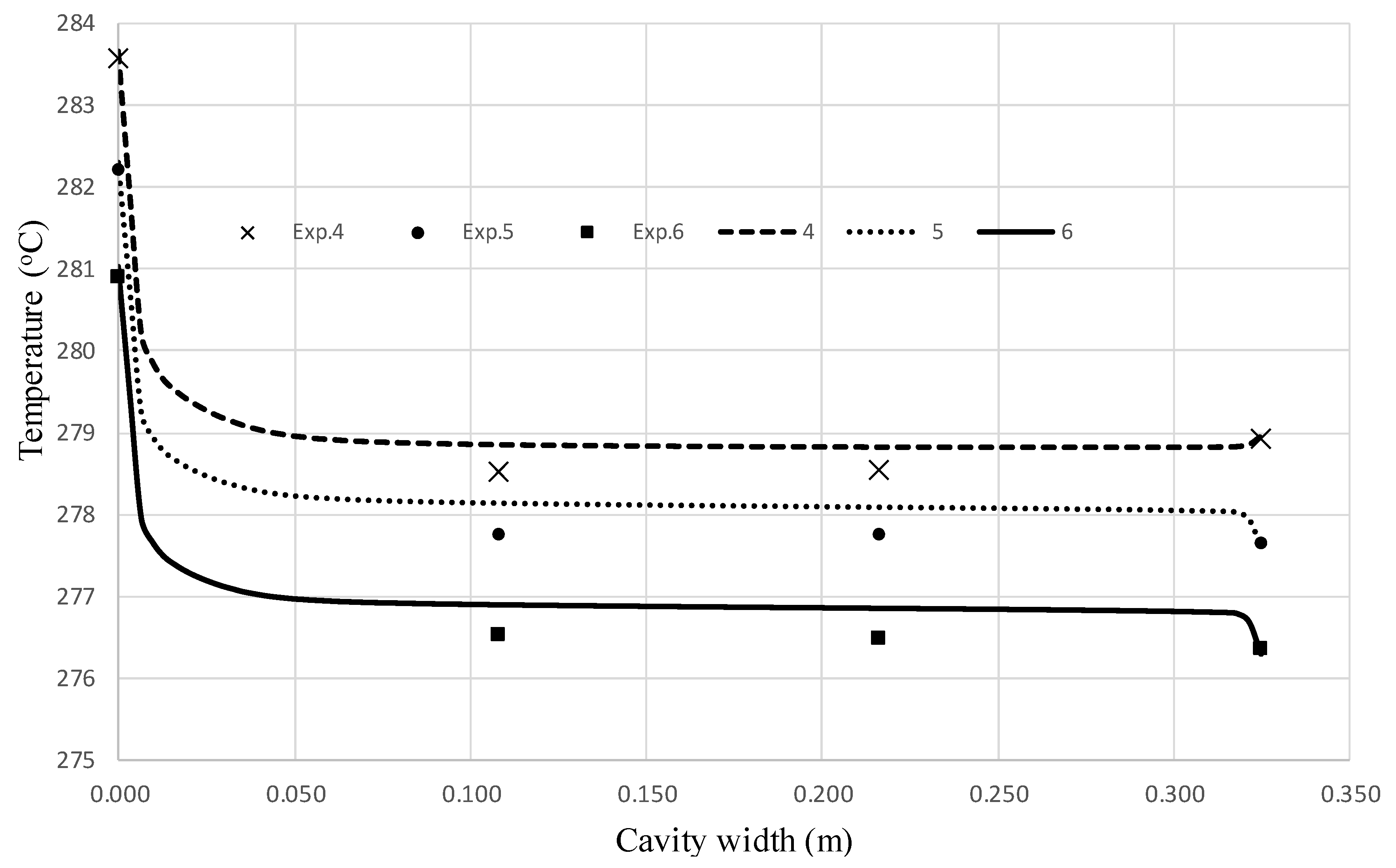
Temperature changes of the air flow and the glass surfaces (primary and secondary façade surfaces) are examined in Figure 5 for different working conditions. For the air temperature in the cavity, measurements which were taken with thermocouples at two levels were compared with the simulation results. It was observed that the numerical model and the experimental measurement results generally behave in coherence with each other. There was a difference at levels of 0.2–0.5 °C in the cavity air temperature for the measurements and simulations for all cavity depths [15]. The main reason of these differences was the heat loss of the cavity air to the laboratory environment even with the well-insulated DSF cavity.
5.3. Velocity Distributions and the Streamlines at the Vertical Section in the Middle of the Cavity
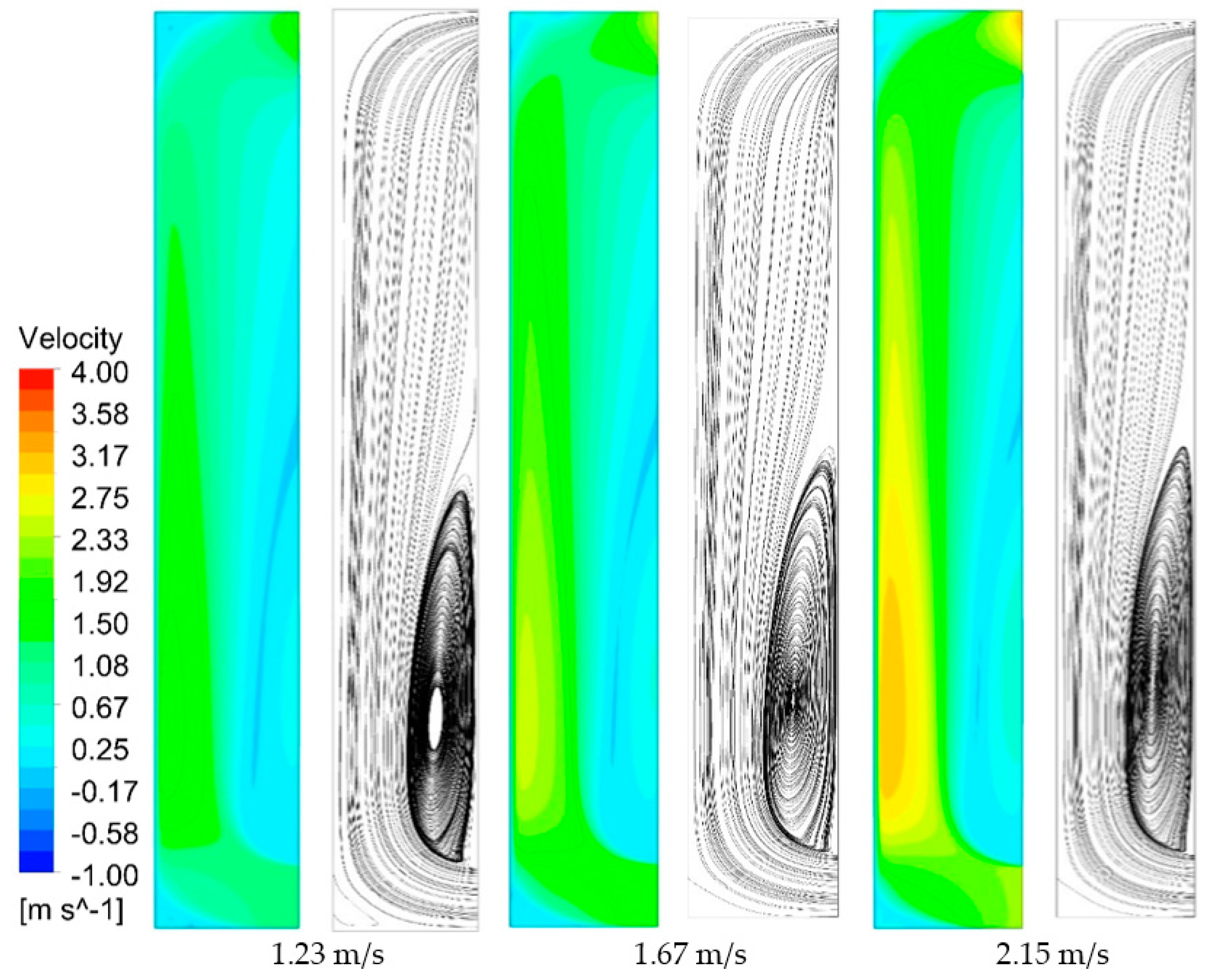
For the condition that the cavity depth was 32.5 cm, depending on different mass flow rates, the velocity distributions and the streamlines in the longitudinal section (mentioned in Figure 2b as a dark colored plane) placed in the middle of the cavity can be seen in Figure 6. In low velocity values, the region in the top section of the cavity with low velocity naturally spanned a larger area comparing to the other parts which had relatively higher velocity. Due to the conditions of entrance and exit to the cavity, the flow mostly rose along the PF surface, maintained at lower values on the SF surface and reverse flows occurred. This circulation zone took the form of a larger loop as the width of the cavity increased. Also, in this process, loops occurred in the corners facing the air entrance and exit vents when the cavity depth was 40 cm [15]. As the velocity increases, this effect becomes more visible. Therefore, as it was emphasized before, in the DSF design, it is important that there should be a slight transition without sharp turns on the corners where these reverse flows occur. This showed the importance of the design of air vents in DSF. With the applications in which the flow was directed to the cavity in the entrance, this negative effect was reduced. It is also important how to choose the appropriate flow rate as much as the design of the air inlet and outlet vent design.
5.4. The Average Pressure Drop at the Vertical Section in the Middle of the Cavity
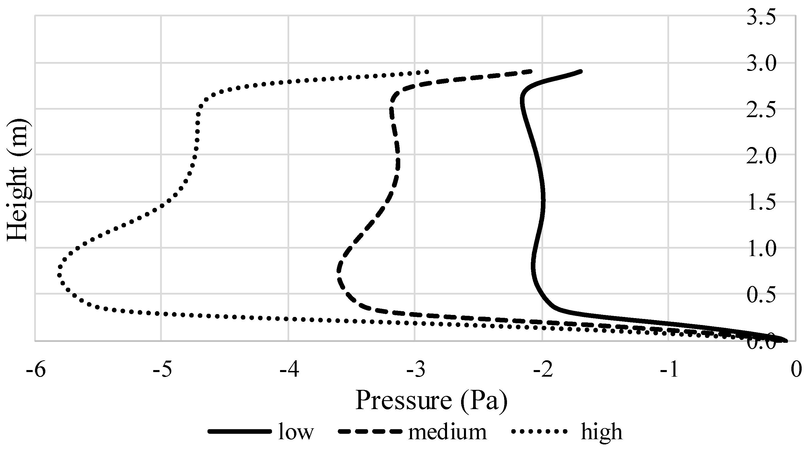
As it was seen from the velocity distributions in the cavity and streamlines, air entrance and exit vents have an important effect on the velocity field. Sharp turns here cause significant pressure drops. This pressure drop increases the required fan capacity and energy consumption together with the possibility of appearance of noise and vibration. For the cavity depth of 32.5 cm, pressure change curves along the cavity which were acquired for three different numerical experiments can be seen in Figure 7. As the cavity width increases, the pressure drop decreases, and with an increase of the velocity in the cavity, pressure drop also increases.
5.5. Temperature Distributions at the Vertical Section in the Middle of the Cavity
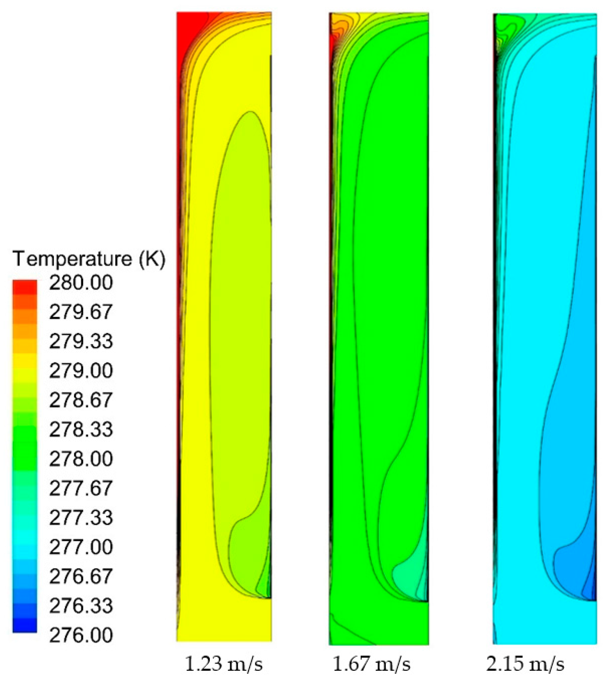
As can be seen in Figure 8, in the section which is close to the air exit vent, there are higher temperature gradients. It is observed that temperature gradients increase as they get closer to the surface of the interior glass (PF) façades due to the relatively higher temperature difference between surface and cavity air temperature. In high flow rate, as the heat convection coefficient value increases, heat transfer from the PF surface to the cavity air also increases. This also explains the importance of the selection of the flow rate in the applications. There is also relatively greater energy exchange between the PF and the cavity air at high velocities. Thus, temperature gradients are more explicit in a wide area of the cavity section.
5.6. Non-Dimensional Correlation Construction between Reynolds and Nusselt Numbers
In all numerical experiments, mass and energy balance were controlled separately and it was observed that they were conserved in each experiment as it can be seen in Table 2. The amount of heat transfer rates from PF and SF are almost equal to the rate of air energy changes (ΔEair) in the cavity and small quantity of energy rates are given as a remaining of numerical calculations shown as ΔEerror. Similarly, inlet and outlet mass flow rates are almost equal each other and there is only a small amount of remaining mass (Table 2). Pressure drops in the cavity are shown in subsequent column. The pressure drop increases with increasing velocity and decreasing cavity width.
Nusselt number, Nu is defined at the PF surface along the cavity height and can be determined as:
where Dh and kair are hydraulic diameter and thermal conductivity of cavity air. h is defined as convection heat transfer coefficient calculated by Equation (10) at the primary facade (PF) surface:
where QPF/APF values along the cavity height at the PF are directly calculated by code as heat fluxes (QPF is given in Table 2). TPF values given in Table 1 are determined experimentally and defined by using a linear equation based on three-point temperature measurements. Tair values along the cavity are the results of running the code.
Nu = h·Dh/kair
h = QPF/[APF(TPF − Tair)]
The Nusselt number changes at the hot surface (PF) along the cavity height are shown in Figure 9 for the numerical experiments numbered 4 to 6. The average Nusselt numbers increase with increasing Reynolds numbers. Heat transfer increased with high temperature changes slightly above from the air inlet of the cavity. Therefore, firstly a sudden increase of the Nusselt number is observed, then the number stabilizes relatively through the cavity. Similar with air inlet, sudden decrease conditions are observed in Nusselt numbers at the air outlet. Due to the flow is in the entrance region thermally along the cavity in all working conditions, the slope of temperature gradient on primary façade decreases along the cavity height (Figure 8). In parallel, Nusselt numbers and heat convection coefficients also decrease depend on temperature gradient. While the cavity air was thermally fully developed towards the end of the cavity (Nu numbers become constant), it decreases at the cavity outlet.
The average Nusselt numbers as well as Reynolds numbers for each experimental case are given in Table 3 for the PF surface of the cavity. Nusselt numbers were acquired by calculating the average value for a 2.0 m portion of the cavity, ranging from 0.5 m to 2.5 m, i.e., without considering the values at the entrance and the exit section. Flow is turbulent in all numerical experiments as shown in Reynolds numbers calculated by using the average velocity values for each situation separately and the hydraulic diameters (Table 3).
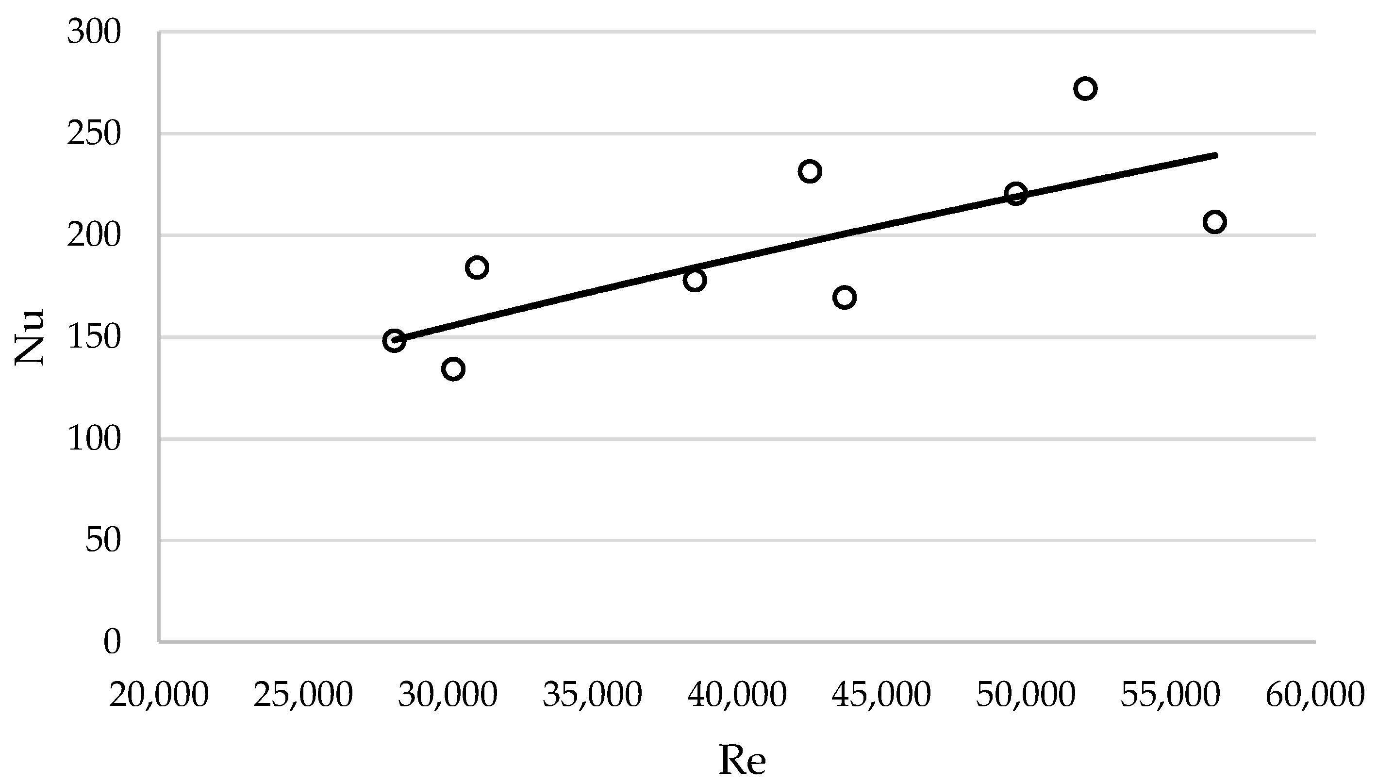
The results given in Table 3 could be generalized by a correlation to predict the heat transfer rate using the Nusselt number for the double skin façade operating with the external air channel condition for Reynolds numbers between 28,000 to 56,500; and 0.10 to 0.16 aspect ratio. Thus, the Nusselt number is a power function of the Reynolds number:
Nu = C·Rem
The Reynolds and Nusselt numbers given in Table 3 were used in a regression analysis to evaluate the indices C and m in Equation (11). By calculating the averages of the low, medium and high flow rates of the all of the cavity depths, Reynolds and Nusselt numbers were computed and a general equation was acquired as shown in Figure 10. Therefore, the correlation for the external air channel condition investigated in this study can be given as:
Nu = 0.1338·Re0.6844
This constructed non-dimensional heat transfer correlation given in Equation (12) can be used to investigate energy analysis of a DSF under defined geometric features and working conditions in this study. This kind of correlations are widely used to identify the convection coefficients of the inner cavity surfaces in the literature [5,24,25,26,27,28]. These correlations are valid under fully developed flow conditions which are the main difference from the current study valid for the entrance region condition hydrodynamically and thermally. Also these studies are more general than the current study covered narrow Re numbers and nonuniform wall temperatures. The correlation given in Equation (12) can be used the box window type of DSF applications having relatively short cavities (except inlet and outlet sections). Convection heat transfer coefficient values are relatively higher in the entrance section than the fully developed conditions. These differences affect the heat transfer rate and must be considered in the energy analysis. Investigation of the air flow and heat transfer of the DSF cavity showed how to change of the convection heat transfer coefficient along the cavity and to affect the heat transfer in the analysis.
6. Conclusions
In this study, experimental and numerical studies were conducted to investigate the flow and heat transfer characteristics through the double skin façade with an external air flow mode. The air cavity between two glass façades designed in the box window type of DSF was evaluated in a test room experimentally. A numerical model was developed to simulate the steady state forced convection inside the DSF cavity after the verification of the numerical studies by using data from the experimental studies. The comparative results showed that the current model could successfully predict the velocity field and temperature variations inside the domain. The following conclusions can be drawn from the current study:
- Forced flow through the DSF cavity were in the thermal and hydrodynamic entrance region for almost all numerical experiments. Thus, convection heat transfer coefficient values for each case were found to be relatively higher in the entrance region except of the inlet and outlet sections. This situation can be considered for the energy analysis of DSF.
- Design of cross section area of air inlet and outlet was significant. Sharp turns created significant pressure drops which increased fan capacity and its energy consumption. This sharp-edged inlet of the cavity behaved like an air flow constriction.
- Recirculating flows around the inlet section created pressure drop and the circulation zone took the form a larger loop as the velocity of the air in the cavity increased.
- Extended data sets from the nine experimental studies under steady-state conditions were collected. These data can be used by the validation of the different numerical studies for a double skin façade with an external airflow mode.
- A correlation based on a Nu-Re analysis of the numerical results was developed to predict the Nusselt numbers with the Reynolds number ranging from 28,000 to 56,500 approximately for a box window type of DSF with an external airflow mode for aspect ratios of 0.10–0.16.
- This non-dimensional correlation could be used to evaluate the energy performance of the double skin façade using climatic data from different locations as a future study.
Acknowledgments
This work was supported by the Scientific and Technological Research Council of Turkey (TÜBİTAK) Foundation under the grant number 112M170.
Author Contributions
Tuğba İnan and Tahsin Başaran designed the experimental setup and performed the experiments. Tuğba İnan, Tahsin Başaran and Aytunç Erek conceived the numerical studies, and Tuğba İnan carried out the numerical experiments. Tuğba İnan and Tahsin Başaran analyzed the experimental and numerical results and wrote the paper.
Conflicts of Interest
The founding sponsors had no role in the design of the study; in the collection, analyses, or interpretation of data; in the writing of the manuscript, and in the decision to publish the results.
Nomenclature
| CA | cavity air |
| C, Cμ, C1ε, C2ε, C3ε | constants |
| cp | specific heat, J/kg K |
| CFD | computational fluid dynamics |
| Dh | hydraulic diameter, m |
| DSF | double skin façade |
| E | energy transfer rate, W |
| Gb | generation of turbulence kinetic energy due to buoyancy |
| Gk | generation of turbulence kinetic energy due to mean velocity gradients |
| h | Convection heat transfer coefficient, W/m2K |
| H | geometric height, m |
| k | thermal conductivity, W/mK; local turbulence kinetic energy |
| L | geometric width, m |
| mass flow rate, kg/s | |
| Nu | Nusselt number |
| p | pressure, Pa |
| PF | primary façade |
| Re | Reynolds number |
| Q | heat transfer rate, W |
| SK, Sε | user-defined source terms |
| SF | secondary façade |
| t | time, s |
| T | temperature, °C |
| u | velocity component, x-direction, m/s |
| v | velocity component, y-direction, m/s |
| V | velocity, m/s |
| w | velocity component, z-direction, m/s |
| W | geometric depth, m |
| YM | contribution of fluctuating dilatation in compressible turbulence to overall dissipation rate |
| x, y, z | cartesian coordinates |
| Greek Symbols | |
| ε | diffusion rate |
| μ | dynamic viscosity, kg/m s |
| ρ | density, kg/m3 |
| σk, σε | turbulent Prandtl numbers for k and ε |
| Δ | differential element |
| Subscripts | |
| avg | average |
| i, j | tensors |
| t | turbulence |
| Superscript | |
| m | constant |
References
- Stec, W.J.; Paassen, A.H.C.; Maziarz, A. Modelling the double skin façade with plants. Energy Build. 2005, 37, 419–427. [Google Scholar] [CrossRef]
- Chou, S.K.; Chua, K.J.; Ho, J.C. A study on the effects of double skin façades on the energy management in buildings. Energy Convers. Manag. 2009, 50, 2275–2281. [Google Scholar] [CrossRef]
- Fuliottoa, R.; Cambulia, F.; Mandasa, N.; Bacchinb, N.; Manarab, G.; Chen, Q. Experimental and numerical analysis of heat transfer and airflow on an interactive building façade. Energy Build. 2010, 42, 23–28. [Google Scholar] [CrossRef]
- Gavan, V.; Woloszyn, M.; Kuznik, F.; Roux, J.J. Experimental study of a mechanically ventilated double-skin façade with Venetian sun-shading device: A full-scale investigation in controlled environment. Sol. Energy 2010, 84, 183–195. [Google Scholar] [CrossRef]
- Bhamjee, M.; Nurick, A.; Madyira, D.M. An experimentally validated mathematical and CFD model of a supply air window: Forced and natural flow. Energy Build. 2013, 57, 289–301. [Google Scholar] [CrossRef]
- Guardo, A.; Coussirat, M.; Valero, C.; Egusquiza, E.; Alavedra, P. CFD assessment of the performance of lateral ventilation in Double Glazed Façades in Mediterranean climates. Energy Build. 2011, 43, 2539–2547. [Google Scholar] [CrossRef]
- Jiru, T.E.; Tao, Y.X.; Haghighat, F. Airflow and heat transfer in double skin façades. Energy Build. 2011, 43, 2760–2766. [Google Scholar] [CrossRef]
- Hazem, A.; Ameghchouche, M.; Bougriou, C. A numerical analysis of the air ventilation management and assessment of the behavior of double skin façades. Energy Build. 2015, 102, 225–236. [Google Scholar] [CrossRef]
- Parra, J.; Guardo, A.; Egusquiza, E.; Alavedra, P. Thermal performance of ventilated double skin façades with venetian blinds. Energies 2015, 8, 4882–4898. [Google Scholar] [CrossRef] [Green Version]
- Radhia, H.; Sharples, S.; Fikiry, F. Will multi-façade systems reduce cooling energy in fully glazed buildings? A scoping study of UAE buildings. Energy Build. 2013, 56, 179–188. [Google Scholar] [CrossRef]
- Darkwa, J.; Li, Y.; Chow, D.H.C. Heat transfer and air movement behavior in a double-skin façade. Sustain. Cities Soc. 2014, 10, 130–139. [Google Scholar] [CrossRef]
- Bejan, A.; Kraus, A.D. Heat Transfer Handbook; John Wiley & Sons: Hoboken, NJ, USA, 2003. [Google Scholar]
- Kakaç, S.; Shah, R.K.; Aung, W. Handbook of Single-Phase Convective Heat Transfer; John Wiley & Sons: New York, NY, USA, 1987. [Google Scholar]
- İnan, T.; Başaran, T.; Ezan, M.A. Experimental and numerical investigation of natural convection in a double skin façade. Appl. Therm. Eng. 2016, 106, 1225–1235. [Google Scholar] [CrossRef]
- İnan, T. Experimental and Numerical Analysis of Flow and Heat Transfer in Double Skin Façade Cavities. Ph.D. Thesis, Department of Architecture, Izmir Institute of Technology, Izmir, Turkey, 2016. [Google Scholar]
- Başaran, T.; İnan, T. Experimental investigation of the pressure loss through a double skin façade by using perforated plates. Energy Build. 2016, 133, 628–639. [Google Scholar] [CrossRef]
- Drikakis, D.; Iliev, O.P.; Vassileva, D.P. A non-linear full multigrid method for the three-dimensional incompressible Navier-Stokes equations. J. Comput. Phys. 1998, 146, 301–321. [Google Scholar] [CrossRef]
- Hahn, M.; Drikakis, D. Large eddy simulation of compressible turbulence using high-resolution methods. Int. J. Numer. Methods Fluids 2005, 47, 971–977. [Google Scholar] [CrossRef]
- Drikakis, D.; Hahn, M.; Mosedale, A.; Thornber, B. Large eddy simulation using high resolution and high order methods. Philos. Trans. R. Soc. A 2009, 367, 2985–2997. [Google Scholar] [CrossRef] [PubMed] [Green Version]
- Kokkinakis, I.W.; Drikakis, D. Implicit large eddy simulation of weakly-compressible turbulent channel flow. Comput. Methods Appl. Mech. Eng. 2015, 287, 229–261. [Google Scholar] [CrossRef] [Green Version]
- ANSYS Inc. Ansys-Fluent 14.0 Theory Guide; ANSYS Inc.: Canonsburg, PA, USA, 2009. [Google Scholar]
- Patankar, S.V. Numerical Heat Transfer and Fluid Flow; Hemisphere: Washington, DC, USA, 1980. [Google Scholar]
- Leonard, B.P.; Mokhtari, S. Ultra-Sharp Nonoscillatory. Convection Schemes for High-Speed Steady Multidimensional Flow; NASA TM 1-2568 (ICOMP-90-12); NASA Lewis Research Center: Cleveland, OH, USA, 1990.
- Jiru, T.E.; Haghighat, F. Modeling ventilated double skin façade—A zonal approach. Energy Build. 2008, 40, 1567–1576. [Google Scholar] [CrossRef]
- Fallahi, A.; Haghighat, F.; Elsadi, H. Energy performance assessment of double-skin façade with thermal mass. Energy Build. 2010, 42, 1499–1509. [Google Scholar] [CrossRef]
- Zanghirella, F.; Perino, M.; Serra, V. A numerical model to evaluate the thermal behaviour of active transparent façades. Energy Build. 2011, 43, 1123–1138. [Google Scholar] [CrossRef]
- Ghadamian, H.; Ghadimi, M.; Shakouri, M.; Moghadasi, M.; Moghadasi, M. Analytical solution for energy modeling of double skin façades building. Energy Build. 2012, 50, 158–165. [Google Scholar] [CrossRef]
- Nastase, G.; Şerban, A.; Dragomir, G.; Bolocan, S.; Brezeanu, A.I. Box window double skin façade. Steady state heat transfer model proposal for energetic audits. Energy Build. 2016, 112, 12–20. [Google Scholar] [CrossRef]
Figure 1.
Experimental setup layout and its main sections.

Figure 2.
The section of DSF cavity. (a) Temperature measurement indication for primary façade (PF), secondary façade (SF) and cavity air (CA) (not to scale); (b) Model geometry with air inlet and outlet cross section areas for numerical study and result plane mentioned vertically.
Figure 2.
The section of DSF cavity. (a) Temperature measurement indication for primary façade (PF), secondary façade (SF) and cavity air (CA) (not to scale); (b) Model geometry with air inlet and outlet cross section areas for numerical study and result plane mentioned vertically.

Figure 3.
Variation of temperature from indoor to the outdoor environment for the 32.5 cm cavity width condition for low flow rate experiment numbered 4, 1300 m3/h.
Figure 3.
Variation of temperature from indoor to the outdoor environment for the 32.5 cm cavity width condition for low flow rate experiment numbered 4, 1300 m3/h.

Figure 4.
Velocity profiles and experimental measurement results (#4) at different cavity heights (Cavity depth: 32.5 cm; low flow rate, 1300 m3/h).
Figure 4.
Velocity profiles and experimental measurement results (#4) at different cavity heights (Cavity depth: 32.5 cm; low flow rate, 1300 m3/h).

Figure 5.
Numerical temperature profiles and their comparison with the experimental (#4–6) results (Cavity depth: 32.5 cm, three different flow rates).
Figure 5.
Numerical temperature profiles and their comparison with the experimental (#4–6) results (Cavity depth: 32.5 cm, three different flow rates).

Figure 6.
Velocity distributions and streamlines in the velocity field in the vertical section through the DSF’s cavity (depth: 32.5 cm) for the numerical experiments numbered 4–6.
Figure 6.
Velocity distributions and streamlines in the velocity field in the vertical section through the DSF’s cavity (depth: 32.5 cm) for the numerical experiments numbered 4–6.

Figure 7.
Pressure drop at the vertical section for the numerical experiments numbered 4–6 (Cavity depth: 32.5 cm).
Figure 7.
Pressure drop at the vertical section for the numerical experiments numbered 4–6 (Cavity depth: 32.5 cm).

Figure 8.
Temperature distributions through the DSF’s cavity for different uniform velocities at the entrance of the cavity (Cavity depth: 32.5 cm).
Figure 8.
Temperature distributions through the DSF’s cavity for different uniform velocities at the entrance of the cavity (Cavity depth: 32.5 cm).

Figure 9.
Variations of the Nusselt numbers at the primary facade’s surface along the cavity height (Cavity depth: 32.5 cm) for the numerical experiments numbered 4–6.
Figure 9.
Variations of the Nusselt numbers at the primary facade’s surface along the cavity height (Cavity depth: 32.5 cm) for the numerical experiments numbered 4–6.

Figure 10.
Nusselt numbers as a function of Reynolds numbers and the relation of Nusselt number as a power function of Reynolds number.
Figure 10.
Nusselt numbers as a function of Reynolds numbers and the relation of Nusselt number as a power function of Reynolds number.


Table 1.
Experimental results.
| Exp. # | Cavity Depth (cm) | Flow | (°C) | (m/s) | PF (°C) | SF (°C) | ||||
|---|---|---|---|---|---|---|---|---|---|---|
| Tinlet | Vinlet | T1,2avg | T3,4avg | T5,6avg | T1,2avg | T3,4avg | T5,6avg | |||
| 1 | 25.0 | low | 4.40 | 1.25 | 6.28 | 8.41 | 9.45 | 3.79 | 4.41 | 4.73 |
| 2 | med | 4.52 | 1.81 | 5.84 | 7.83 | 8.60 | 3.53 | 4.01 | 4.31 | |
| 3 | high | 3.34 | 2.34 | 4.53 | 6.45 | 7.13 | 2.30 | 2.56 | 2.89 | |
| 4 | 32.5 | low | 5.71 | 1.23 | 7.45 | 9.22 | 10.41 | 4.95 | 5.44 | 5.78 |
| 5 | med | 5.03 | 1.67 | 6.31 | 7.98 | 9.06 | 3.84 | 4.11 | 4.49 | |
| 6 | high | 3.78 | 2.15 | 5.03 | 6.76 | 7.76 | 2.66 | 2.78 | 3.20 | |
| 7 | 40.0 | low | 6.40 | 1.40 | 8.30 | 10.14 | 11.34 | 5.53 | 5.95 | 6.33 |
| 8 | med | 6.36 | 1.92 | 7.86 | 9.58 | 10.58 | 5.15 | 5.29 | 5.63 | |
| 9 | high | 5.89 | 2.35 | 7.18 | 8.84 | 9.76 | 4.75 | 4.60 | 4.92 | |
Table 2.
Numerical experiment results: Energy and mass balances and CFD outputs as outlet temperature and pressure drop for the cavity.
Table 2.
Numerical experiment results: Energy and mass balances and CFD outputs as outlet temperature and pressure drop for the cavity.
| Exp. # | (K) | Q (W) | Pascal | ṁ (kg/s) | |||||
|---|---|---|---|---|---|---|---|---|---|
| Toutlet | PF | SF | ΔEair | ΔEerror | Δp | ṁinlet | ṁoutlet | Δṁ | |
| 1 | 277.82 | 119.900 | −1.017 | 118.573 | −0.310 | 1.753 | 0.44204980 | 0.44204962 | 1.788 × 10⁻⁷ |
| 2 | 277.83 | 124.700 | 19.994 | 104.285 | −0.421 | 3.152 | 0.64110140 | 0.64110191 | −5.364 × 10⁻⁷ |
| 3 | 276.62 | 142.023 | −30.802 | 110.551 | −0.670 | 4.608 | 0.83308649 | 0.83308619 | 2.980 × 10⁻⁷ |
| 4 | 279.06 | 94.339 | −7.224 | 86.773 | −0.342 | 1.878 | 0.43359959 | 0.43359985 | −2.682 × 10⁻⁷ |
| 5 | 278.30 | 98.098 | −25.357 | 72.265 | −0.477 | 2.635 | 0.59128022 | 0.59128016 | 5.960 × 10⁻⁸ |
| 6 | 277.05 | 120.811 | −29.322 | 90.900 | −0.589 | 3.867 | 0.76466095 | 0.76466018 | 7.749 × 10⁻⁷ |
| 7 | 279.73 | 100.283 | −10.254 | 89.612 | −0.418 | 1.937 | 0.49215615 | 0.49215606 | 8.941 × 10⁻⁸ |
| 8 | 279.63 | 108.603 | −26.712 | 81.446 | −0.445 | 2.780 | 0.67640877 | 0.67640847 | 2.980 × 10⁻⁷ |
| 9 | 279.14 | 116.771 | −34.663 | 81.458 | −0.650 | 3.565 | 0.83000046 | 0.83000070 | −2.384 × 10⁻⁷ |
Table 3.
Average Nusselt numbers calculated numerically and Reynolds numbers determined experimentally.
Table 3.
Average Nusselt numbers calculated numerically and Reynolds numbers determined experimentally.
| Exp. # | #1 | #2 | #3 | #4 | #5 | #6 | #7 | #8 | #9 |
|---|---|---|---|---|---|---|---|---|---|
| C. Depth (cm) | 25.0 | 32.5 | 40.0 | ||||||
| Re | 30,190 | 43,720 | 56,530 | 28,150 | 38,540 | 49,650 | 31,010 | 42,520 | 52,050 |
| Nu | 134.29 | 169.45 | 206.59 | 148.17 | 177.88 | 220.39 | 184.10 | 231.38 | 272.10 |
© 2017 by the authors. Licensee MDPI, Basel, Switzerland. This article is an open access article distributed under the terms and conditions of the Creative Commons Attribution (CC BY) license (http://creativecommons.org/licenses/by/4.0/).
Share and Cite
MDPI and ACS Style
İnan, T.; Başaran, T.; Erek, A. Experimental and Numerical Investigation of Forced Convection in a Double Skin Façade. Energies 2017, 10, 1364. https://doi.org/10.3390/en10091364
AMA Style
İnan T, Başaran T, Erek A. Experimental and Numerical Investigation of Forced Convection in a Double Skin Façade. Energies. 2017; 10(9):1364. https://doi.org/10.3390/en10091364
Chicago/Turabian Styleİnan, Tuğba, Tahsin Başaran, and Aytunç Erek. 2017. "Experimental and Numerical Investigation of Forced Convection in a Double Skin Façade" Energies 10, no. 9: 1364. https://doi.org/10.3390/en10091364
Note that from the first issue of 2016, this journal uses article numbers instead of page numbers. See further details here.