A Quadratic Fractional Map without Equilibria: Bifurcation, 0–1 Test, Complexity, Entropy, and Control

Abstract

Fractional calculus in discrete-time systems is a recent research topic. The fractional maps introduced in the literature often display chaotic attractors belonging to the class of “self-excited attractors”. The field of fractional map with “hidden attractors” is completely unexplored. Based on these considerations, this paper presents the first example of fractional map without equilibria showing a number of hidden attractors for different values of the fractional order. The presence of the chaotic hidden attractors is validated via the computation of bifurcation diagrams, maximum Lyapunov exponent, 0–1 test, phase diagrams, complexity, and entropy. Finally, an active controller with the aim for stabilizing the proposed fractional map is successfully designed.

1. Introduction

Continuous-time and discrete-time chaotic dynamical systems have been extensively studied over the last few years [1], and a large number of papers on chaos control, synchronization, and chaos application has been introduced continuously [2,3]. Chaotic microelectromechanical resonator model has been analyzed in [3]. Multistability has been observed in a chaotic system with two circles of equilibrium points [4]. The digital chaotic oscillator has been designed and implemented [5]. Complex dynamics of a memristor-based chaotic circuit has been reported in [6]. It is noted that Nozaki et al. studied nonlinear control system applied to atomic force microscope including parametric errors [7]. Referring to continuous-time systems, the most common type of attractors are the so-called “self-excited attractors”, for which the initial conditions are located close to the saddle points of the chaotic flow [8,9]. However, chaos can be generated also in systems without saddle points—for example, in systems characterized by the absence of equilibria [10] or by the presence of stable equilibria only [11]. These types of attractors are the so-called “hidden attractors”, for which the initial conditions can only be found via extensive numerical search [12]. Consequently, these types of chaotic attractors are difficult to be discovered [13]. Referring to discrete-time systems, the topic of chaotic maps characterized by “hidden attractors” has been only recently investigated [14,15,16]. For example, in [14], a 1D chaotic discontinuous map without equilibria has been illustrated, whereas, in [15], 2D and 3D chaotic maps with different types of stable equilibria have been proposed. Moreover, 2D chaotic quadratic maps without equilibria and with no discontinuity in the right-hand equations have been introduced in [16]. After deriving a simple detailed explanation about the procedure of designing such systems with quadratic nonlinearities and continuous right-hand side function, the authors systematically investigated the complex dynamical behaviors of these maps using numerical simulation.

The previous considerations are related to integer-order chaotic systems. However, over the last few years, several efforts have been devoted to the study of fractional-order chaotic systems, i.e., both continuous-time systems described by fractional-order differential equations [17,18] and discrete-time systems described by fractional-order difference equations [19,20]. Referring to the latter systems, a number of fractional-order chaotic maps has been recently introduced [21,22,23,24]. For example, in [21] 3D Stefanski, Rössler, and Wang fractional maps have been illustrated, whereas, in [22], a novel 3D generalized Hénon map is analyzed. Moreover, in [23], the fractional-order version of the Grassi–Miller map is considered, whereas, in [24], the dynamics of the fractional discrete double scroll are analyzed in detail.

It should be noted that the mentioned fractional maps show chaotic attractors belonging to the class of “self-excited attractors”. To the best of the authors’ knowledge, no fractional map showing “hidden attractors” has been introduced in the literature to date. Based on these considerations, this paper presents a fractional map without equilibria on the basis of reference [16], which shows a number of hidden attractors for different values of the fractional order in the difference equations. The presence of the chaotic hidden attractors is validated via the bifurcation diagrams, the computation of the maximum Lyapunov exponent, and the 0–1 test. Additionally, the complexity (that reflects the irregularity in the discrete data) and the entropy (that quantifies the amount of regularity and the unpredictability of fluctuations in the data) are carefully evaluated and analyzed. The paper is organized as follows. In Section 2, by exploiting the Caputo difference operator, a 2D fractional-order map with no discontinuity in the right-hand equations is introduced. In particular, it is shown that there is no equilibrium point in the system dynamics for any value of the bifurcation parameters. In Section 3, bifurcation diagrams, maximum Lyapunov exponent, 0–1 test, phase diagrams, complexity, and entropy are computed and discussed. Finally, an active controller with the aim of stabilizing the proposed fractional map is designed in Section 4.

2. A Fractional-Order Map without Equilibria

Recently, Panahi et al. [16] proposed a simple two-dimensional chaotic map with no equilibrium point and with quadratic nonlinearities. The mathematical model of the map is defined as:

$$\left\{\begin{array}{c}{x}_{n+1}=y_n+x_n,\hfill \\ y_{n+1}=0.1x_n^2+0.1+y_n[-x_n-b{y}_n]+y_n,\hfill \end{array}\right.$$

(1)

where x, y are state variables and b is the bifurcation parameter. The chaotic attractors of this map are hidden. The phase space, bifurcation diagram, and Lyapunov exponents are plotted in Figure 1 confirming the existence of chaos. In order to derive the fractional version of (1), we start by taking the the first–order difference as

$$\left\{\begin{array}{c}\Delta x_n=y_n,\hfill \\ \Delta y_n=0.1x_n^2-b{y}_n^2-y_n{x}_n+0.1.\hfill \end{array}\right.$$

(2)

Let us first recall some of the necessary fractional discrete operators such as fractional sum and Caputo type delta difference.

Definition 1.

Let $X\left(t\right):{\mathbb{N}}_a\to \mathbb{R}$ with ${\mathbb{N}}_a=\left\{a,a+1,a+2,\dots \right\}$ and $\nu >0,$ we define the fractional sum of $X\left(t\right)$ with order ν as [25]:

$${\Delta }_a^{-\nu }X\left(t\right)=\frac{1}{\mathrm{\Gamma }\left(\nu \right)}\sum _{s=a}^{t-\nu }{\left(t-s-1\right)}^{\left(\nu -1\right)}X\left(s\right).$$

(3)

Note that the term $t^{\left(\nu \right)}$ is known as the falling function and may be defined by means of the Γ-function as

$$t^{\left(\nu \right)}=\frac{\mathrm{\Gamma }\left(t+1\right)}{\mathrm{\Gamma }\left(t+1-\nu \right)}.$$

(4)

Definition 2.

For $X\left(t\right):{\mathbb{N}}_{a+n-\nu }\to \mathbb{R}$ and $\nu \notin \mathbb{N}$, the Caputo difference operator of $X\left(t\right)$ with order ν is given as [26]:

$${}^C{\Delta }_a^{\nu }X\left(t\right)={\Delta }_a^{-(n-\nu )}{\Delta }^{\nu }X\left(t\right)=\frac{1}{\mathrm{\Gamma }\left(n-\nu \right)}\sum _{s=a}^{t-\left(n-\nu \right)}{\left(t-s-1\right)}^{\left(n-\nu -1\right)}{\Delta }_s^{n}X\left(s\right),$$

(5)

where $n=⌈\nu ⌉+1$.

By introducing the ${}^C{\Delta }_a^{\nu }$ operator in the integer order difference Equation (2), the fractional-order map with order $\nu \in ]0,1]$ is given as:

$$\left\{\begin{array}{c}{}^C{\Delta }_a^{\nu }x\left(t\right)=y(t-1+\nu ),\hfill \\ {}^C{\Delta }_a^{\nu }y\left(t\right)=0.1x^2(t-1+\nu )-b{y}^2(t-1+\nu )-x(t-1+\nu )y(t-1+\nu )+0.1,\hfill \end{array}\right.$$

(6)

where a is the starting point and $t\in N_{a+1-\nu }$. We denote the equilibrium point of the fractional-order map (6) with $(x_e,y_e)$. The equilibrium point of the fractional-order map (6) can be found by solving

$$\left\{\begin{array}{c}{}^C{\Delta }_a^{\nu }{x}_e=y_e,\hfill \\ {}^C{\Delta }_a^{\nu }{y}_e=0.1x_e^2-b{y}_e^2-x_e{y}_e+0.1,\hfill \end{array}\right.$$

(7)

and by taking in mind that the Caputo-like delta difference of constant is equal to zero, we get:

$$0.1\left(x_e^2+1\right)=0.$$

Therefore, there is no any equilibrium point in the fractional-order map (6) for any value of the bifurcation parameter $b.$

3. Chaos Analysis

In the following, we will mainly discuss the chaotic behavior of the fractional-order map (6) using simulation experiments, including phase portraits, bifurcation diagrams, and maximum Lyapunov exponents. In addition, some tests of chaos such as the 0–1 test, $C_0$ complexity, and entropy are added to see the performance of our numerical results. To continue with our analysis, we need to recall the following theorem which will allow us to define the numerical formula of the proposed system.

Theorem 1.

[27] For the fractional difference equation,

$$\left\{\begin{array}{c}{}^C{\Delta }_a^{\nu }u\left(t\right)=f(t+\nu -1,u(t+\nu -1)),\hfill \\ {\Delta }^{k}u\left(a\right)=u_k,n=⌈\nu ⌉+1,k=0,1,\dots ,n-1,\hfill \end{array}\right.$$

(8)

the equivalent discrete integral equation can be obtained as

$$u\left(t\right)=u_0\left(t\right)+\frac{1}{\mathrm{\Gamma }\left(\nu \right)}\sum _{s=a+n-\nu }^{t-\nu }{(t-s-1)}^{(\nu -1)}f(s+\nu -1,u(s+\nu -1)),t\in {\mathbb{N}}_{a+n},$$

(9)

where

$$u_0\left(t\right)=\sum _{k=0}^{n-1}\frac{{(t-a)}^{\left(k\right)}}{\mathrm{\Gamma }\left(k+1\right)}{\Delta }^{k}u\left(a\right).$$

(10)

Using Theorem 1 and assuming that $a=0$, the system (6) is converted to:

$$\left\{\begin{array}{c}x\left(n\right)=x\left(0\right)+\frac{1}{\mathrm{\Gamma }\left(\nu \right)}\sum _{j=1}^n\frac{\mathrm{\Gamma }\left(n-j+\nu \right)}{\mathrm{\Gamma }\left(n-j+1\right)}\left(y\left(j-1\right)\right),\hfill \\ y\left(n\right)=y\left(0\right)+\frac{1}{\mathrm{\Gamma }\left(\nu \right)}\sum _{j=1}^n\frac{\mathrm{\Gamma }\left(n-j+\nu \right)}{\mathrm{\Gamma }\left(n-j+1\right)}\hfill \\ \times \left(0.1x^2(j-1)-b{y}^2(j-1)-x(j-1)y(j-1)+0.1\right).\hfill \end{array}\right.$$

(11)

This numerical formula will allow us to examine the sensitivity of the fractional-order map (6) throughout the remainder of this paper.

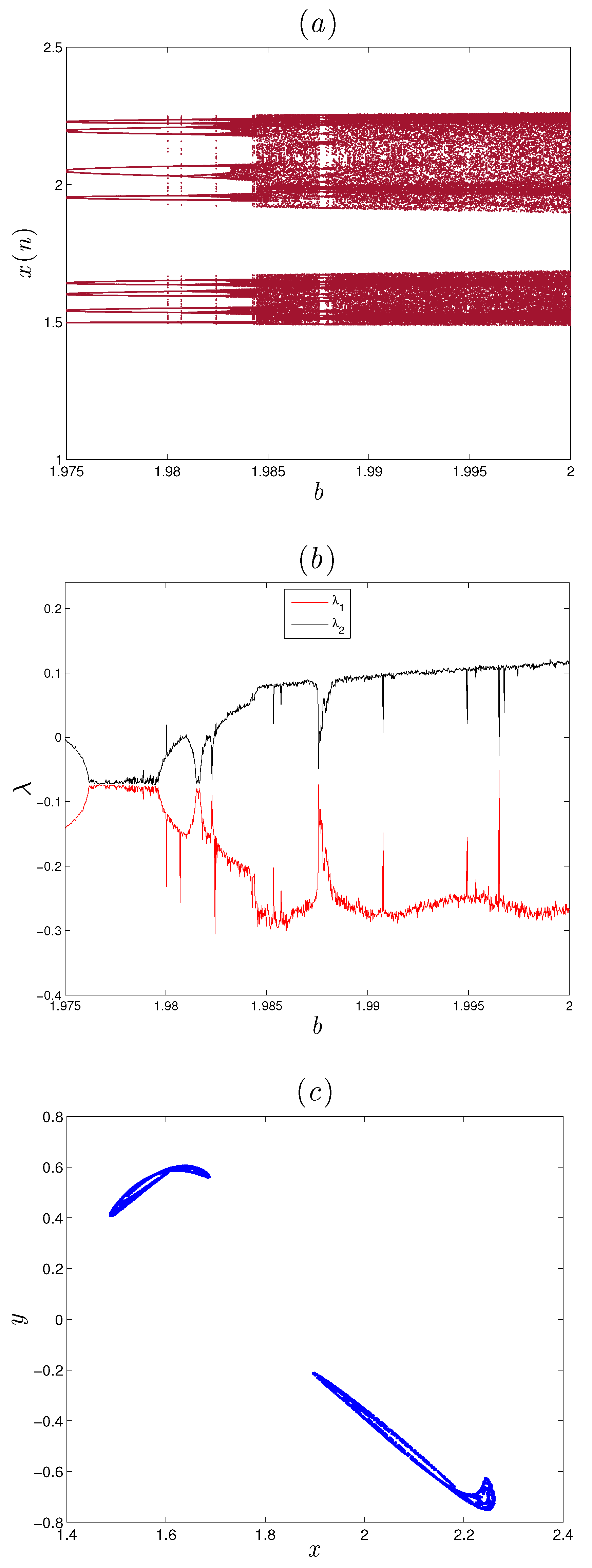
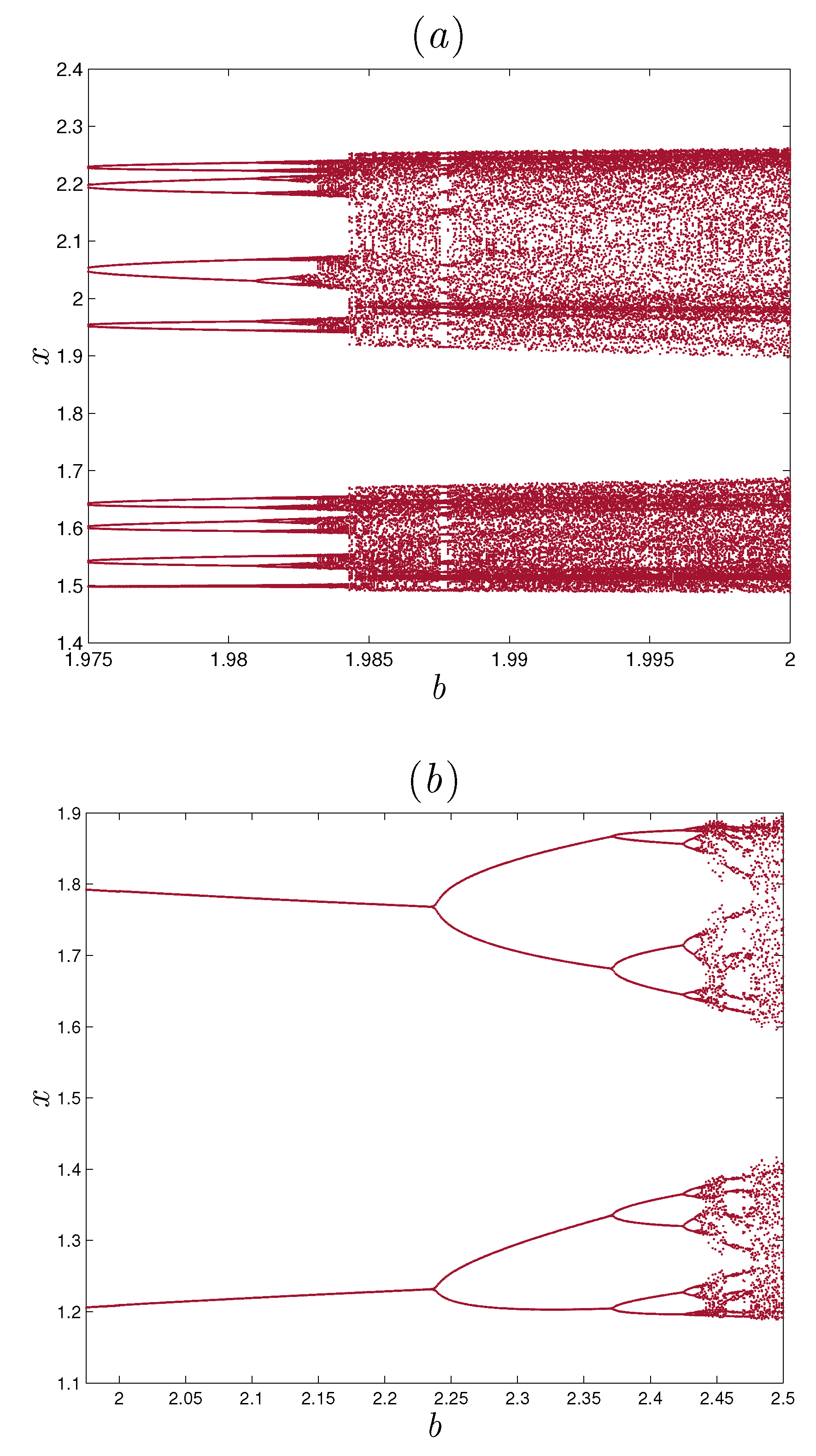
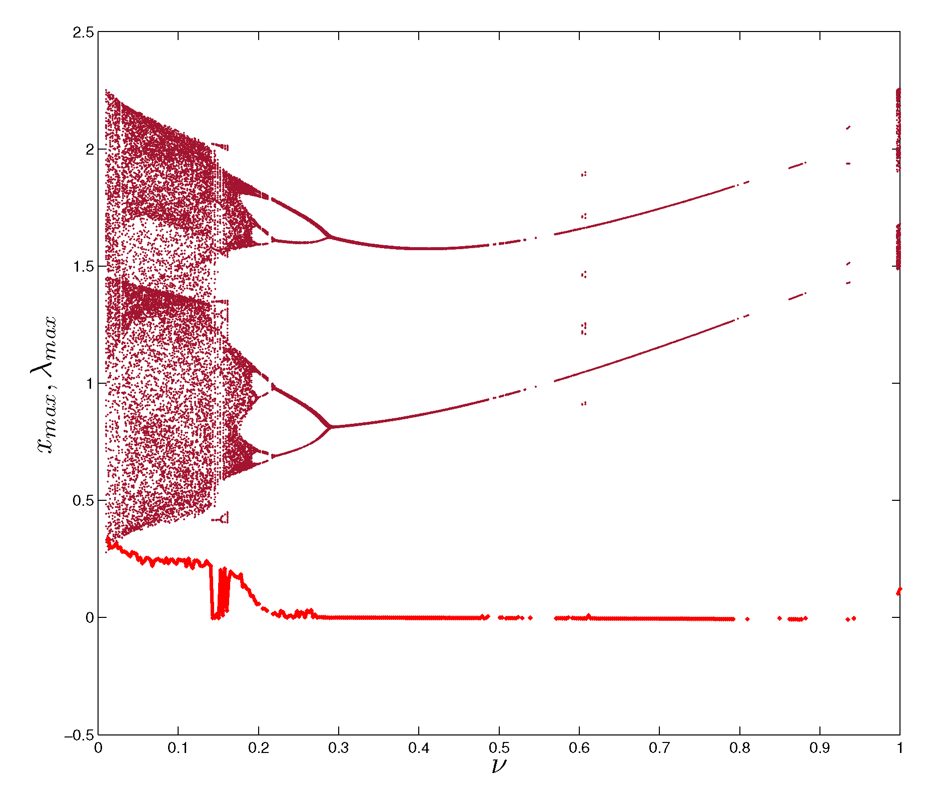
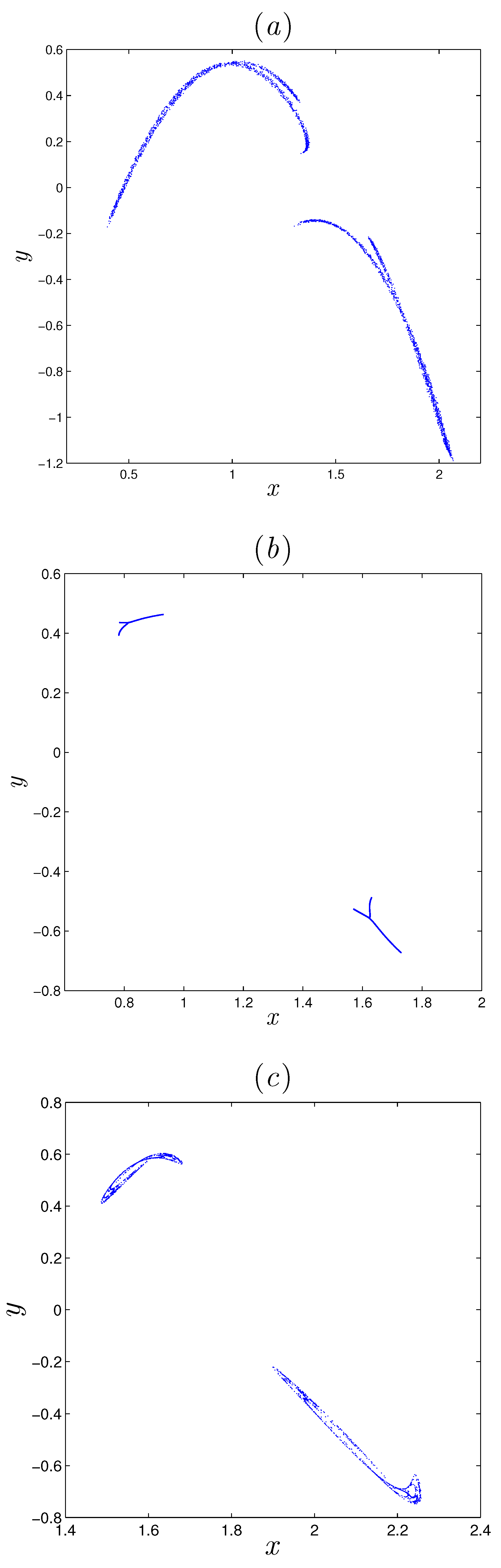
3.1. Bifurcations and Maximum Lyapunov Exponents

This subsection is devoted to analyze the dynamic properties of the fractional-order map (6). Consider the dynamic evolution of system (6) with respect to parameter b under the given initial condition $(x_0,y_0)=(1.7,-0.39)$. The bifurcation diagrams of the fractional-order map (6) for two different values of $\nu$ are shown in Figure 2. As it can be seen, the variation of order $\nu$ has a critical impact on the states of the fractional-order map (6). Figure 2a is the bifurcation diagram of system (6) with order $\nu =1$. When $b\in [1.975,1.983]$, a series of periodic windows is observed. As we range b from $1.983$ to 2, the states of the fractional-order map (6) display chaotic dynamics. In the bifurcation diagram of Figure 2b, we use the fractional order value $\nu =0.7457$. In this case, the route leading to chaos is a period doubling bifurcation. Comparing this diagrams, it can be seen that the area of chaotic motions decreases as the order $\nu$ varied. Now, we consider the effect of $\nu$ on the dynamic behavior of the fractional-order map (6) for $b=2$. Figure 3 shows the resulting bifurcation diagram. Clearly, a period doubling scenario route to chaos is observed as $\nu$ decreases. In this case, the fractional-order map is chaotic when $\nu \in ]0.01,0.1962[\cup [0.996,1]$, while it is regular in the remaining interval. To validate this, the maximum Lyapunov exponent is calculated using the Jacobian matrix algorithm [28]. As is well known, a system is verified to be chaotic when the maximum Lyapunov exponent (LE) is positive. The maximum LE diagram which is associated with Figure 3 is reported with a red line. In Figure 3, the maximum Lyapunov exponent is equal to zero or negative over most of the rang $(0.1962,0.996)$, which implies that the fractional-order map is periodic. For small values of $\nu$, the fractional-order map is more complex because the corresponding maximum LE is larger. The phase diagrams with several specified values of fractional order are plotted in Figure 4. From Figure 4, we can see that there are different and new hidden chaotic attractors, which is consistent with the results in Figure 3.

3.2. 0–1 Test

In this subsection, we justified the existence of chaos by means of a 0–1 test method. The 0–1 test for chaos is a relatively new method that is applied directly to a series of data and does not require phase space reconstruction. Based on the state $x\left(n\right)$ of the numerical formula (11), we define the translation variables $p_c\left(n\right)={\sum }_{j=1}^{n}x\left(j\right)\cos \left(jc\right)$ and $q_c\left(n\right)={\sum }_{j=1}^{n}x\left(j\right)\sin \left(jc\right),$ for $n=1,\dots ,n$, with c being randomly chosen from the interval $(0,2\pi )$. To determine whether chaos occurs, we can simply plot $q_c$ and $p_c$ in the the two-dimensional $(p_c-q_c)$ plane. Namely, Brownian-like trajectories imply chaos, whereas bounded trajectories imply regular dynamics. Next, we compute the mean square displacement $M_c\left(n\right)$ as follows:

$$M_c\left(n\right)=\underset{N\to \infty }{\lim }\frac{1}{N}\sum _{j=1}^N{\left[p_c(j+n)-p_c\left(j\right)\right]}^2+{\left[q_c(j+n)-q_c\left(j\right)\right]}^2.$$

(12)

From this one, we can define the asymptotic growth rate $K_c$ for random number c as:

$$K_c=\underset{n\to \infty }{\lim }\frac{\log M_c\left(n\right)}{\log \left(n\right)}.$$

(13)

Finally, we define K as the median of all $K_c$ values for which $K=1$ signifies chaos while $K=0$ describes the regular dynamics.

Table 1. Results of the 0–1 test for the fractional order map (6) with different fractional order values.

$\nu$	0.06767	0.0852	0.2931	0.4244	0.998
K	0.996	0.901	−0.0015	−0.00762	0.7633

and Figure 5 depict the results of the test for different values of $\nu$ with $b=2$. We observe that, when $\nu =0.06767,\nu =0.0852$ and $\nu =0.998$, the asymptotic growth rate K of the fractional order map are $K=0.996$, $K=0.901$, and $K=0.7633$, respectively. Additionally, the unbounded behavior of the translation component in the $p-q$ plane (Figure 5) shows Brownian-like trajectories which indicates chaos. These results agree well with the phase diagrams in Figure 4. Conversely, for $\nu =0.2931$, the 0–1 test approaches 0 and returns bounded trajectories as shown in Figure 5b, confirming that the fractional order map is periodic for $\nu =0.2931$.

3.3. $C_0$ Complexity

The $C_0$ complexity is an index that can describe the random degree of a discrete data [29]. This algorithm is described as follows. Considering the state $\left\{x\right(n),n=0,1,2,\dots ,N-1\}$ of the fractional-order map (6), its corresponding Fourier transformation is computed by

$${\psi }_N\left(j\right)=\frac{1}{N}\sum _{k=0}^{N-1}x\left(j\right){\exp }^{-2\pi i\left(\frac{kj}{N}\right)},j=0,1,2,\dots ,N-1,$$

(14)

where j is the imaginary unit. Next, calculate the mean square value of ${\psi }_N$ as:

$$G_N=\frac{1}{N}\sum _{j=0}^{N-1}{\left|{\psi }_N\left(j\right)\right|}^2,$$

(15)

and let

$${\overline{\psi }}_N\left(j\right)=\left\{\begin{array}{cc}{\psi }_N\left(j\right),\hfill & \mathrm{if}{\left|{\psi }_N\left(j\right)\right|}^2>r{G}_N,\hfill \\ 0\hfill & \mathrm{if}{\left|{\psi }_N\left(j\right)\right|}^2\le r{G}_N,\hfill \end{array}\right.$$

(16)

where r is a control parameter. Thus, $C_0$ complexity is defined as:

$$C_0=\frac{{\sum }_{k=0}^{N-1}{\left|x\left(k\right)-\overline{x}\left(k\right)\right|}^2}{{\sum }_{k=0}^{N-1}{\left|x\left(k\right)\right|}^2}.$$

(17)

The $C_0$ complexity of state $x\left(n\right)$ of the numerical formula (11) is calculated versus order $\nu$ as shown in Figure 6. Figure 6 presents that the complexity of the fractional order map (6) decreases with the increment of the fractional order $\nu$, which agrees with the results in Figure 3.

3.4. Approximate Entropy

Now, the complexity of the fractional-order map (6) is described by employing approximate entropy (ApEn), which is briefly described as follows. Given n set of discrete data $x\left(1\right),x\left(2\right),\dots ,x\left(n\right)$ obtained from the fractional-order map (6), for a given m, form a sequence of vectors $X\left(j\right)$ for $j=1,\dots ,n-m+1$ as $X\left(j\right)=\left(x\right(j),\dots ,x(j+m-1\left)\right)$. These vectors represent m consecutive x values, starting with the $i-$th point. Define the distance $d\left(X\right(i),X(j\left)\right)$ between vectors $X\left(i\right)$ and $X\left(j\right)$ as the maximum difference in their respective scalar components. For a given $X\left(i\right)$, count the number of j so that $d\left(X\right(i),X(j\left)\right)\le r$ is denoted as K, the relative frequency of $X\left(i\right)$ being similar to $X\left(j\right)$ is:

$$C_i^m\left(r\right)=\frac{K}{n-m+1}.$$

(18)

The approximate entropy [30] is defined by

$$ApEn={\varphi }^m\left(r\right)-{\varphi }^{m+1}\left(r\right),$$

(19)

where ${\varphi }^m\left(r\right)$ is considered as

$${\varphi }^m\left(r\right)=\frac{1}{n-m-1}\sum _{i=1}^{n-m+1}\log C_i^m\left(r\right).$$

(20)

Let $b=2$ and $(x_0,y_0)=(1.7,-0.39)$, Figure 7 shows the ApEn of the proposed fractional-order map (6) for different fractional order values. As one can see, the complexity of the fractional-order map (6) varied as we change $\nu$. Therefore, we must be aware of the selected fractional order in order to have a relatively high structural complexity. The fractional-order map (6) is more complex when $\nu \in (0.1253,0.1353)$.

4. Chaos Control

For the purpose of stabilizing the fractional-order map (6), we design an active controller in this section. First, let us present the following theorem reported in [31], which provides the basis for the stability conditions of the zero solution of a fractional-order map.

Theorem 2.

The zero equilibrium of the linear fractional-order discrete–time system

$${}^C{\Delta }_a^{\nu }X\left(t\right)=\mathbf{M}X\left(t+\nu -1\right),$$

(21)

where $X\left(t\right)={\left(x_1\left(t\right),\dots ,x_n\left(t\right)\right)}^T,$ $0<\nu \le 1,$ $\mathbf{M}\in {\mathbb{R}}^{n\times n}$ and $\forall t\in {\mathbb{N}}_{a+1-\nu },$ is asymptotically stable if

$$\lambda \in \left\{z\in \mathbb{C}:\left|z\right|<{\left(2\cos \frac{\left|\arg z\right|-\pi }{2-\nu }\right)}^{\nu }\mathit{and}\left|\arg z\right|>\frac{\nu \pi }{2}\right\},$$

(22)

for all the eigenvalues λ of $\mathbf{M}$.

The states of the fractional-order map (6) with controller $({\mathbf{C}}_1$,${\mathbf{C}}_2{)}^T$ are described as:

$$\left\{\begin{array}{c}{}^C{\Delta }_a^{\nu }x\left(t\right)=y(t-1+\nu )+{\mathbf{C}}_1,\hfill \\ {}^C{\Delta }_a^{\nu }y\left(t\right)=0.1x^2(t-1+\nu )-b{y}^2(t-1+\nu )-x(t-1+\nu )y(t-1+\nu )+0.1+{\mathbf{C}}_2.\hfill \end{array}\right.$$

(23)

Here, our goal is to design a suitable controller to assure that all states of the fractional-order map converge to zero asymptotically. For that, we propose the following theorem.

Theorem 3.

The two–dimensional fractional-order map (6) is stabilized under the following two–dimensional control law described by

$$\left\{\begin{array}{c}{\mathbf{C}}_1=-x\left(t\right),\hfill \\ {\mathbf{C}}_2=-y\left(t\right)-0.1x^2\left(t\right)+b{y}^2\left(t\right)+x\left(t\right)y\left(t\right)-0.1.\hfill \end{array}\right.$$

(24)

Proof. 

Substituting the proposed control law (21) into the system (22) yields the simplified dynamics

$${}^C{\Delta }_a^{\nu }{\left(x\left(t\right),y\left(t\right)\right)}^T=\mathbf{M}\times {\left(x\left(t-1+\nu \right),y\left(t-1+\nu \right)\right)}^T,$$

(25)

where

$$\mathbf{M}=\left(\begin{array}{cc}-1& 1\\ 0& -1\end{array}\right).$$

(26)

Based on the stability results of linear fractional-order maps Theorem 2, the zero equilibrium point of the system (25) is asymptotically stable if the eigenvalues ${\lambda }_1$, ${\lambda }_2$ of the matrix $\mathbf{M}$ satisfy

$$\left|\arg {\lambda }_i\right|=\pi >\frac{\nu \pi }{2}\mathrm{and}\left|{\lambda }_i\right|=1<{\left(2\cos \frac{\left|\arg {\lambda }_i\right|-\pi }{2-\nu }\right)}^{\nu },i=1,2.$$

Clearly, the above condition is fulfilled, which means that the zero equilibrium of the system (23) is asymptotically stable. Hence, the states are guaranteed to converge to zero asymptotically.  □

In order to validate the result of Theorem 3, one can set the system (23) with $b=2$, $a=0$, and fractional order $\nu =0.998$, and the evolution of states is displayed in Figure 8. Obviously, Figure 8 shows clearly that the states converge rapidly towards zero, which confirms the result very well.

5. Conclusions

Since the field of fractional map showing “hidden attractors” is completely unexplored in the literature, this paper has made a contribution to the topic by presenting the first example of fractional map without equilibria. The proposed fractional difference equations exploit the Caputo operator and do not contain any discontinuity on their right-hand side. The conducted analysis has shown that the map possesses a number of hidden attractors for different values of the fractional order in the difference equations. Bifurcation diagrams, maximum Lyapunov exponent, 0–1 test, phase diagrams, complexity, and entropy have been computed in order to highlight the effectiveness of the proposed approach. Finally, an active controller for stabilizing the system dynamics has been successfully designed. The influence of parametric errors will be studied in our future works. It is believed that the proposed no equilibrium fractional-order map will contribute to the development of the theoretical study of fractional-order maps with hidden attractors. Moreover, it has the potential application of being used in several scientific and engineering fields.

References

1. Sprott, J.C. Elegant Chaos: Algebraically Simple Chaotic Flows; World Scientific: Singapore, 2010. [Google Scholar]
2. Tusset, A.M.; Balthazar, J.M.; Rocha, R.T.; Ribeiro, M.A.; Lenz, W.B. On suppression of chaotic motion of a nonlinear MEMS oscillator. Nonlinear Dyn. 2020, 99, 537–557. [Google Scholar] [CrossRef]
3. Bassinello, D.G.; Tusset, A.M.; Rocha, R.T.; Balthazar, J.M. Dynamical analysis and control of a chaotic microelectromechanical resonator model. Shock Vibration 2018, 2018, 4641629. [Google Scholar] [CrossRef] [Green Version]
4. Sambas, A.; Vaidyanathan, S.; Tlelo-Cuautle, E.; Zhang, S.; Guillen-Fernandez, O.; Hidayat, Y.S.; Gundara, G. A novel chaotic system with two circles of equilibrium points: Multistability, electronic circuit and FPGA realization. Electronic 2019, 8, 1211. [Google Scholar] [CrossRef] [Green Version]
5. Berviller, Y.; Tisserand, E.; Poure, P.; Rabah, H. Design and implementation of a digital dual orthogonal outputs chaotic oscillator. Electronis 2020, 9, 264. [Google Scholar] [CrossRef] [Green Version]
6. Song, Q.; Chang, H.; Li, Y. Complex dynamics of a novel chaotic system based on an active memristor. Electronis 2020, 9, 410. [Google Scholar] [CrossRef] [Green Version]
7. Nozaki, R.; Balthazar, J.M.; Tusset, A.M.; de Pontes , B.R., Jr.; Bueno, A.M. Nonlinear control system applied to atomic force microscope including parametric errors. J. Control Autom. Electr. Sys. 2013, 24, 223–231. [Google Scholar] [CrossRef]
8. Leonov, G.A.; Kuznetsov, N.V.; Vagaitsev, V.I. Hidden attractor in smooth Chua systems. Phys. D Nonlinear Phenom. 2012, 241, 1482–1486. [Google Scholar] [CrossRef]
9. Leonov, G.A.; Kuznetsov, N.V.; Kiseleva, M.A.; Solovyeva, E.P.; Zaretskiy, A.M. Hidden oscillations in mathematical model of drilling system actuated by induction motor with a wound rotor. Nonlinear Dyn. 2014, 77, 277–288. [Google Scholar] [CrossRef]
10. Wei, Z. Dynamical behaviors of a chaotic system with no equilibria. Phys. Lett. A 2011, 376, 102–108. [Google Scholar] [CrossRef]
11. Molaie, M.; Jafari, S.; Sprott, J.C.; Golpayegani, S.M.R.H. Simple chaotic flows with one stable equilibrium. Int. J. Bifurc. Chaos 2013, 23, 1350188. [Google Scholar] [CrossRef]
12. Leonov, G.A.; Kuznetsov, N.V. Hidden attractors in dynamical systems. From hidden oscillations in Hilbert–Kolmogorov, Aizerman, and Kalman problems to hidden chaotic attractor in Chua circuits. Int. J. Bifurc. Chaos 2013, 23, 1330002. [Google Scholar] [CrossRef] [Green Version]
13. Sharma, P.R.; Shrimali, M.D.; Prasad, A.; Kuznetsov, N.V.; Leonov, G.A. Controlling dynamics of hidden attractors. Int. J. Bifurc. Chaos 2015, 25, 1550061. [Google Scholar] [CrossRef]
14. Jafari, S.; Pham, V.T.; Golpayegani, S.M.R.H.; Moghtadaei, M.; Kingni, S.T. The relationship between chaotic maps and some chaotic systems with hidden attractors. Int. J. Bifurc. Chaos 2016, 26, 1650211. [Google Scholar] [CrossRef]
15. Jiang, H.; Liu, Y.; Wei, Z.; Zhang, L. A new class of three-dimensional maps with hidden chaotic dynamics. Int. J. Bifurc. Chaos 2016, 26, 1650206. [Google Scholar] [CrossRef]
16. Panahi, S.; Sprott, J.C.; Jafari, S. Two simplest quadratic chaotic maps without equilibrium. Int. J. Bifurc. Chaos 2018, 28, 1850144. [Google Scholar] [CrossRef]
17. Wen, G.; Grassi, G.; Feng, Z.; Liu, X. Special issue on advances in nonlinear dynamics and control. J. Franklin Inst. 2015, 8, 2985–2986. [Google Scholar] [CrossRef]
18. Azar, A.T.; Vaidyanathan, S.; Ouannas, A. (Eds.) Fractional Order Control and Synchronization of Chaotic Systems; Springer: Cham, Switzerland, 2017; Volume 688. [Google Scholar]
19. Ouannas, A.; Khennaoui, A.A.; Odibat, Z.; Pham, V.T.; Grassi, G. On the dynamics, control and synchronization of fractional-order Ikeda map. Chaos Solitons Fractals 2019, 123, 108–115. [Google Scholar] [CrossRef]
20. Khennaoui, A.A.; Ouannas, A.; Bendoukha, S.; Grassi, G.; Lozi, R.P.; Pham, V.T. On fractional–order discrete–time systems: Chaos, stabilization and synchronization. Chaos Solitons Fractals 2019, 119, 150–162. [Google Scholar] [CrossRef]
21. Khennaoui, A.A.; Ouannas, A.; Bendoukha, S.; Grassi, G.; Wang, X.; Pham, V.T.; Alsaadi, F.E. Chaos, control, and synchronization in some fractional-order difference equations. Adv. Differ. Equ. 2019, 2019, 1–23. [Google Scholar] [CrossRef] [Green Version]
22. Jouini, L.; Ouannas, A.; Khennaoui, A.A.; Wang, X.; Grassi, G.; Pham, V.T. The fractional form of a new three-dimensional generalized Hénon map. Adv. Differ. Equ. 2019, 2019, 122. [Google Scholar] [CrossRef]
23. Ouannas, A.; Khennaoui, A.A.; Grassi, G.; Bendoukha, S. On chaos in the fractional-order Grassi–Miller map and its control. J. Comput. Appl. Math. 2019, 358, 293–305. [Google Scholar] [CrossRef]
24. Ouannas, A.; Khennaoui, A.A.; Bendoukha, S.; Grassi, G. On the Dynamics and Control of a Fractional Form of the Discrete Double Scroll. Int. J. Bifurc. Chaos 2019, 29, 1950078. [Google Scholar] [CrossRef]
25. Atici, F.M.; Eloe, P.W. Discrete fractional calculus with the nabla operator. Electr. J. Qual. Theory Differ. Equ. 2009, 2009, 1–12. [Google Scholar] [CrossRef]
26. Abdeljawad, T. On Riemann and Caputo fractional differences. Comp. Math. Appl. 2011, 62, 1602–1611. [Google Scholar] [CrossRef] [Green Version]
27. Anastassiou, G.A. Principles of delta fractional calculus on time scales and inequalities. Math. Comp. Modell. 2010, 52, 556–566. [Google Scholar] [CrossRef]
28. Wu, G.C.; Baleanu, D. Jacobian matrix algorithm for Lyapunov exponents of the discrete fractional maps. Commun. Nonlinear Sci. Numer. Simulat. 2015, 22, 95–100. [Google Scholar] [CrossRef]
29. En-Hua, S.; Zhi-Jie, C.; Fan-Ji, G. Mathematical foundation of a new complexity measure. Appl. Math. Mech. 2005, 26, 1188–1196. [Google Scholar] [CrossRef]
30. Pincus, S.M. Approximate entropy as a measure of system complexity. Proc. Natl. Acad. Sci. USA 1991, 88, 2297–2301. [Google Scholar] [CrossRef] [Green Version]
31. Cermak, J.; Gyori, I.; Nechvatal, L. On explicit stability conditions for a linear fractional difference system. Fract. Calc. Appl. Anal. 2015, 18, 651–672. [Google Scholar] [CrossRef]
Figure 1. Numerical analysis of system (1) with ( x 0 , y 0 ) = ( 1.7 0.39 ) : (a) bifurcation diagram with the variation of b; (b) Lyapunov exponents with variation of b; (c) hidden chaotic attractor for b = 2 .
Electronics 09 00748 g001
Figure 2. Bifurcation diagrams of the fractional-order map (6) when the parameter b is varied with the different values of order ν : (a) for ν = 1 ; (b) for ν = 0.7457 .
Electronics 09 00748 g002
Figure 3. Bifurcation diagram and largest Lyapunov exponent of the fractional-order map (6) when the fractional order ν is varied with b = 0.2 .
Electronics 09 00748 g003
Figure 4. Hidden attractors for different values of ν : (a) Hidden chaotic attractor for ν = 0.0852 ; (b) Hidden periodic attractor for ν = 0.2931 ; (c) Hidden chaotic attractor for ν = 0.998 .
Electronics 09 00748 g004
Figure 5. Dynamics of the translation components p q for the fractional order map (6) different values of ν : (a) ν = 0.0852 , (b) ν = 0.2931 , (c) ν = 0.998 .
Electronics 09 00748 g005
Figure 6. C o complexity of the fractional order map (6) with ν varying and b = 2 .
Electronics 09 00748 g006
Figure 7. ApEn of the fractional-order map (6) with ν varying and b = 2 .
Electronics 09 00748 g007
Figure 8. State and Phase trajectories of the fractional order map (6) after control: (a) evolution of state x ( n ) ; (b) evolution of state y ( n ) ; (c) phase space.
Electronics 09 00748 g008