Scan Matching by Cross-Correlation and Differential Evolution

Abstract

Scan matching is an important task, solved in the context of many high-level problems including pose estimation, indoor localization, simultaneous localization and mapping and others. Methods that are accurate and adaptive and at the same time computationally efficient are required to enable location-based services in autonomous mobile devices. Such devices usually have a wide range of high-resolution sensors but only a limited processing power and constrained energy supply. This work introduces a novel high-level scan matching strategy that uses a combination of two advanced algorithms recently used in this field: cross-correlation and differential evolution. The cross-correlation between two laser range scans is used as an efficient measure of scan alignment and the differential evolution algorithm is used to search for the parameters of a transformation that aligns the scans. The proposed method was experimentally validated and showed good ability to match laser range scans taken shortly after each other and an excellent ability to match laser range scans taken with longer time intervals between them.

1. Introduction

The determination of the position of a moving object is an essential part of many complex applications. While outdoor localization can be achieved with the help of global satellite networks including the Global Positioning System (GPS) and the Global Navigation Satellite System (GLONASS), an efficient indoor localization is still an open problem [1,2]. It can be defined as the process of obtaining the location of a moving object in an indoor environment [2]. Indoor localization is an enabling technology for a variety of location-based services that can be used in the context of advanced manufacturing (Industry 4.0) [3], Internet of things [2], smart buildings [1], indoor (underground) rescue operations [4,5] and many other applications.

Self-localization of an autonomous mobile robot or an unmanned aerial vehicle (UAV) [6], a special type of indoor localization, is one of the great challenges of modern robotics [7,8]. It relies on an independent measurement and analysis of sensor data that performed by the robot to estimate its own position and motion trajectory in an unknown indoor environment. In contrast to other types of indoor localization, it does not use any external signals, beacons or other information than is not sensed by the robot itself [8]. Self-localization is associated with the problem of simultaneous localization and mapping (SLAM). As SLAM, it requires approaches that are accurate, robust and computationally efficient at the same time [8].

There are many methods of mobile robot indoor self-localization [2,7,9,10,11]. In general, they are based on video signals analysis and computer vision, infrared and ultrasound sensors, laser range finders, sonar systems [7,12], radio-frequency identification (RFID), wireless network technologies such as Wi-Fi, Bluetooth [10,11] and Zigbee [2], ultra-wideband (UWB), magnetic sensors and acoustic signal analysis [2,10]. Indoor self-localization by light detection and ranging (LiDAR) relies on analysis of a sequence of laser range scans. The scans capture the surroundings of the robot as a series of points representing the intersections of the laser beam with nearby objects [7]. They generate sequences of 2- or 3-dimensional point clouds that are mutually compared (matched) to approximate the trajectory of the robot in the environment. In general, scan matching algorithms can be split into two major groups. Point-based approaches process the entire point clouds, while feature-based techniques focus on features extracted from the point clouds by various feature extraction algorithms. The features are seen as landmarks and the changes in their (relative) locations are used to estimate the moves of the robot [7].

Advanced methods that utilize artificial intelligence, machine learning and soft computing can be used for different types of self-localization applications. For example, artificial neural networks and support vector machines have been used to build indoor localization models based on the received signal strength indicator (RSSI) [2]. In this work, a novel scan matching algorithm based on differential evolution and modified cross-correlation is introduced. Cross-correlation is used to evaluate the alignment of laser range scans, while differential evolution serves as an optimization method for the approximation of the scan matching parameters.

The contributions of this work are twofold: (1) It shows that the differential evolution can be used as an optimization mechanism in a point-based scan matching strategy; and (2) It demonstrates that cross-correlation is a computationally efficient and at the same time robust point cloud alignment measure. The extensive experimental evaluation of these novel concepts also demonstrates that the scan matching procedure based on differential evolution and cross-correlation can be used for accurate indoor localization of autonomous mobile devices.

The remainder of this article is structured in the following way. The problem of localization is summarized and related work is reviewed in Section 2. The algorithms used in this work (scan matching, cross-correlation and differential evolution) are described in Section 3. The proposed approach is detailed in Section 4 and experimentally evaluated in Section 5. The results of conducted experiments are discussed in Section 6 and the article is concluded in Section 7 which also outlines future research directions.

2. Related Work

Although indoor localization has been addressed by a plethora of methods and algorithms with various properties, it still remains an open problem. Tightly linked to mapping of (unknown) indoor environments, it is an essential element of the compound problem of simultaneous localization and mapping (SLAM) [13,14]. Different types of localization and SLAM algorithms have been developed for various types of environments [15]. Accurate SLAM algorithms have been proposed for large outdoor areas [16] and limited indoor spaces [17]. Monte Carlo localization (MCL) is a popular family of localization methods [9,18,19] that use, among others, particle and Kalman filters [20]. At the starting point of the MCL process, a pool of random positions and angles is created. When the robot moves through an environment, the algorithm updates all positions in the pool according to a robot motion model. The expected robot surrounding is compared to data from a sensor (e.g., the LiDAR) surveying the actual environment and the positions that correspond to the real data most are rewarded. The disadvantage of the MCL method is the necessity for robot movement and the need for additional sensors (e.g., odometers) that are required by the motion model [21].

Another family of promising SLAM approaches is based on the use of event cameras [22]. Event cameras produce sequences of video frames and, additionally, information about brightness changes on the pixel level. The advantages of event cameras include very high dynamic range, absence of motion blur and only a small latency (in the order of microseconds [23]). An overview of SLAM algorithms that use event cameras is provided, for example, in [24].

Localization is also one of the major challenges of UAVs. They require information about precise location in to order to avoid obstacles [25] and for trajectory planning [26]. UAVs can, in general, implement similar localization approaches as mobile robots. However, the localization methods need to be adjusted to address the specifics of aerial movement such as 3D SLAM. A comprehensive review of localization strategies for UAVs can be found in [6].

Scan matching [27,28] is a group of popular high-level localization/SLAM methods that process laser range scans of an environment [29]. They align two laser range scans of the (usually unknown) environment in order to detect the change of the location and orientation of a moving object [30]. Scan matching algorithms can be classified as point-based and feature-based. Point-based methods process laser range scans point-by-point whereas feature-base methods extract higher-level features such as lines, corners and so forth, and align these features. Feature-based methods extract distinctive features before matching itself and thus decrease the amount of data that needs to be processed. As a result, their scan matching phase has lower computational costs but they suffer from lower robustness and worse accuracy in rich and well-structured environments.

Iterative closest point (ICP) is a typical representative of point-based scan matching algorithms [31]. ICP is a seminal method that has a number of modifications [32,33]. A representative of feature-based scan matching strategies is the complete line segment (CLS) method [34]. It looks for flat areas in point clouds, extracts lines and detects complete and incomplete line segments. It expects that a complete line segment in an environment has a specific constant length from any point of view. Other feature-based scan matching strategies include the anchor point relationships (APR) algorithm [35] that detects specific anchors, plane extraction approaches [36] and keypoint and keyline extraction [37].

Nature-inspired methods, such as evolutionary computation, have been used in the area of mobile robot localization as well. In [38], the differential evolution algorithm was used in conjunction with the traditional normal distribution transform (NDT) algorithm [39]. Another work used differential evolution as part of a feature-based scan matching algorithm that extracted lines, planes and spheres from laser range scans [40]. Other nature-inspired methods such as the harmonic search algorithm were used for differential scan matching as well [41].

This work proposes a novel scan matching algorithm based on a combination of two recently introduced approaches. The cross-correlation approach [42,43] is adopted for the assessment of laser range scans’ similarity and the differential evolution is used for the search of accurate laser range scan transformation parameters [44]. The evaluation of the proposed scan matching strategy is performed in a series of simulation experiments with the help of a software framework introduced in [45].

3. Background

This section provides the background of the presented work. It outlines the simulation-based design strategy it adopts, relevant scan matching methods such as the iterative closest point algorithm, the fundamentals of the cross-correlation principle and the optimization process implemented by the differential evolution.

3.1. Experimental Setup and Embedded Data Processing

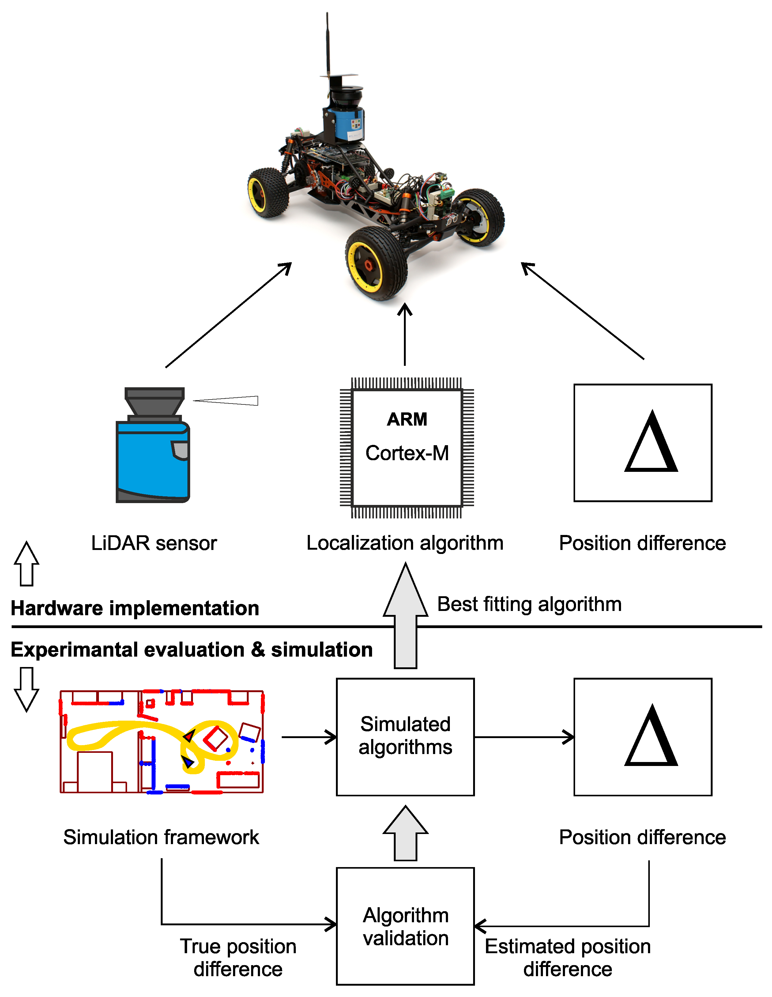
The aim of this work is the design of a localization algorithm suitable for an autonomous mobile vehicle, for example a wheeled mini robot for exploration, surveillance and rescue operations. Hardware architecture of such vehicle was described, for example, in [46]. The mechanical construction of the vehicle was based on the RC Baja 5B SS chassis and it was equipped with all necessary electronic devices that allowed the control of its movement. The vehicle was also equipped with the SICK LMS 100 LiDAR and a set of odometry sensors.

A novel algorithm for a specific system or device ought to be validated in terms of correctness, accuracy, reliability and robustness. In order to allow rapid prototyping and evaluation of various approaches, a model-based development using a software simulation of particular system components (i.e., Software in the Loop) was adopted to validate the scan matching algorithm. The simulation framework provides information about the true position and orientation of the device, simulates its movement in a pre-defined indoor environment and produces simulated LiDAR and odometry data. The structure of the environment is defined by a floor plan. The target processor is an Advanced RISC Machine (ARM) Cortex-M microcontroller expected to run the scan matching algorithm and to compute the estimated position and orientation of the device in the real device. This top–level design strategy is visually illustrated in Figure 1.

An ARM Cortex-M processor supports different functionality depending on its version.

Table 1. Overview of various ARM Cortex-M features useful for computational localization.

	ARM Cortex-M Version	M0+	M3	M4	M7
Architecture	CPU architecture	Von Neumann	Harvard	Harvard	Harvard
	Pipeline stages	2	3	3	6
Integer operations	MULT 32 bit	Fast/Slow	Fast	Fast	Fast
	DIV 32 bit	No	Yes	Yes	Yes
	DSP	No	No	Yes	Yes
Floating-point operations	FPU single precision	No	No	Optional	Optional
	FPU double precision	No	No	No	Optional

describes the basic features of several recent ARM Cortex-M versions (M0+, M3, M4 and M7) [47]. In general, the proposed approach makes use of summation, multiplication and division operations that can be implemented as integer or floating-point operations.

The performance of a processor can be assessed from three different perspectives. An ARM Cortex-M processor can implement the von Neumann or the Harvard architecture. The Harvard architecture has a separate instruction bus connected to an internal cross-bar bus. It supports hardware parallelism by allowing simultaneous access to instructions and data. The second important property of the implemented architecture is the number of stages in the instruction pipeline. A higher number of pipeline stages can accelerate instruction execution and increase the computational power of a processor. For integer operations, the processor implements an add instruction as a standard functionality of an arithmetic logic unit (ALU). However, multiply, divide and digital signal processing (DSP) instructions are optional. ARM Cortex-M family processors can be equipped with slow (32 cycles) or fast (1 cycle) multiply instructions, 32-bit divide instructions and digital signal processing instructions (e.g., a multiply–accumulate operation) useful for input signal filtering. If the executed algorithm uses floating-point data types, then the presence of a floating-point unit (FPU) is highly recommended due to the long processing times without this mathematical co-processor. An FPU can be realized in the processor core as a single (32-bit) or a double (64-bit) precision version of a mathematical co-processor.

The selection of a suitable processor core version depends not only on data-type implementation but there are several important algorithm parameters including the resolution of input data, grid map cell size and the type and configuration of the optimization procedure.

3.2. Scan Matching

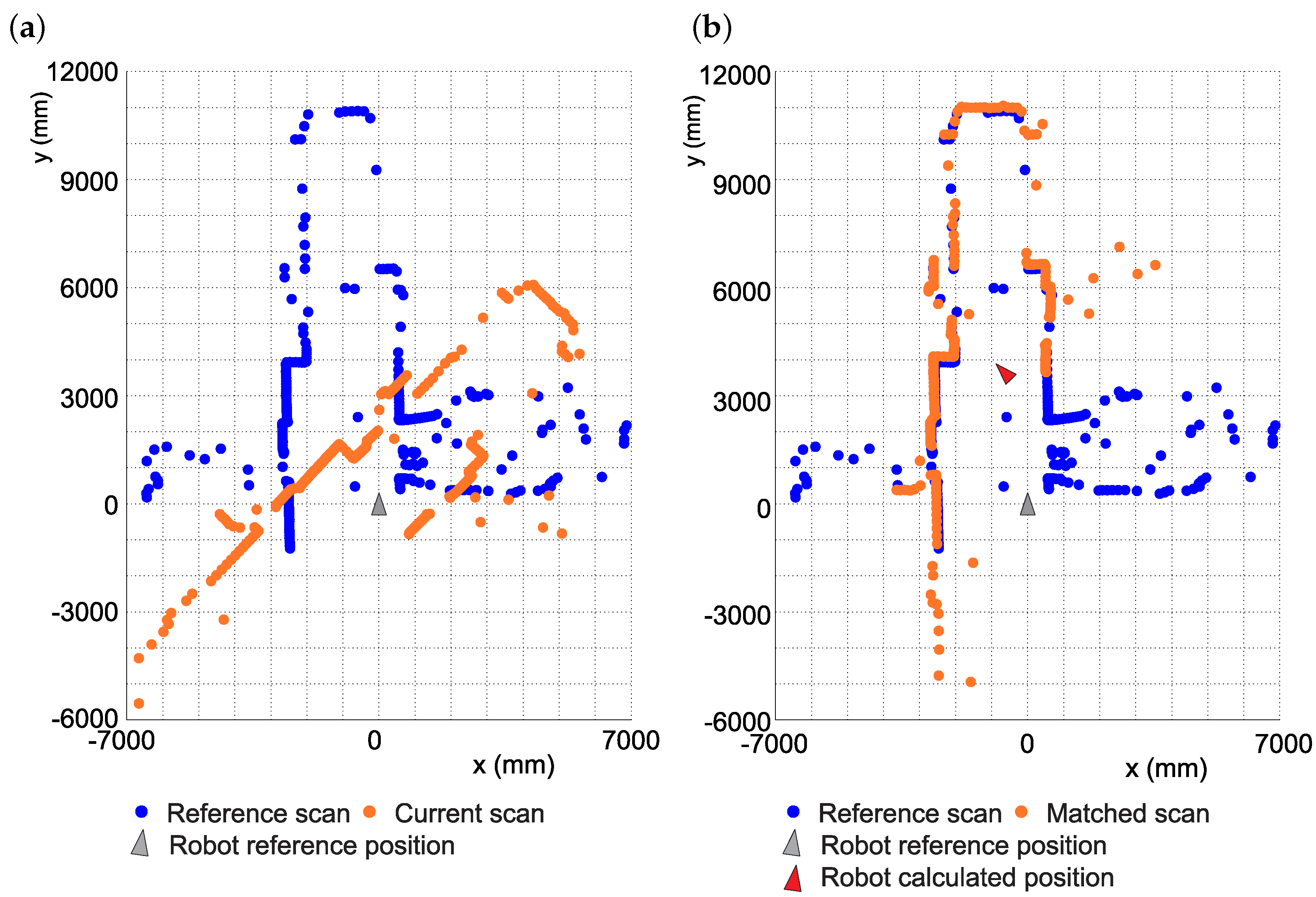
Scan matching is a high-level self-localization strategy based on the assumption that two spatio-temporally collocated laser range scans of an environment are alike and can be (to a large extent) aligned [48]. Scan matching methods seek transformations that align two laser range scans taken by a robot in the same environment but at different locations and from a different angle. The first laser range scan, taken at the first location, is usually called the reference scan and the second laser range scan, taken at the second location, is called the current scan. The transformation that aligns the scans is defined by parameters that describe the relative position and rotation of the scan (see Figure 2). Figure 2a shows two laser range scans before the transformation (alignment) and Figure 2b shows the same scans after a successful alignment.

Scan matching is most often based on 2 or 3-dimensional point clouds captured by LiDAR laser rangefinders. The LiDAR periodically measures the distance to the nearest object in the direction of a laser beam it emits [48]. In a 2-dimensional LiDAR, the measuring laser beam is rotated on the horizontal plane and creates a laser range scan that corresponds to the surrounding of the scanner [49]. 3-dimensional LiDARs also tilt the measuring sensor in the vertical direction and obtain 3-dimensional point clouds [50]. A typical 2-dimensional LiDAR laser range finder, also used in this study, is Sick LMS 100 by SICK AG. This type of range scanner produces counterclockwise oriented vectors of distances to the nearest obstacle. The output of the scanner is a range vector,

$$\overrightarrow{a}=\langle |a_1|,|a_2|,\cdots ,|a_{s_{max}}|\rangle ,$$

(1)

composed of a sequence of distances to the nearest objects, $|a_1|,|a_2|,\cdots ,|a_{s_{max}}|$ and $s_{max}$ is the number of measurement steps within the aperture range of the scanner. Each measured distance, $|a_{{\varphi }_i}|$, corresponds to a particular angle, ${\varphi }_i$ and each range vector, $\overrightarrow{a}$, corresponds to a vector of angles,

$$\overrightarrow{\varphi }=\langle {\varphi }_1,{\varphi }_2,\cdots ,{\varphi }_{s_{max}}\rangle ,$$

(2)

where the index of the angle corresponds to the orientation of the laser beam. The range vector, $\overrightarrow{a}$, together with the angle vector, $\overrightarrow{\varphi }$, describe the surrounding of the scanner in the polar coordinate system. The laser range scan, $(\overrightarrow{a},\overrightarrow{\varphi })$, can be transformed to the Cartesian coordinates by

$$\mathbf{A}=\left(\begin{array}{c}\langle \left|a_1\right|·cos\left({\varphi }_1\right),\left|a_2\right|·cos\left({\varphi }_2\right),\cdots ,\left|a_{s_{max}}\right|·cos\left({\varphi }_{s_{max}}\right)\rangle \hfill \\ \langle \left|a_1\right|·sin\left({\varphi }_1\right),\left|a_2\right|·sin\left({\varphi }_2\right),\cdots ,\left|a_{s_{max}}\right|·sin\left({\varphi }_{s_{max}}\right)\rangle \hfill \end{array}\right),$$

(3)

where $\mathbf{A}\in {\mathbb{R}}^{2\times s_{max}}$ is a real matrix with the first row representing the x coordinates and the second row to the y coordinates of the points in the scan expressed in Cartesian coordinates. Each column of $\mathbf{A}$, ${\overrightarrow{a}}_s\in \mathbf{A}$, corresponds to a single point of the scan in Cartesian coordinates:

$${\overrightarrow{a}}_s=\left(\begin{array}{c}{a}_x\hfill \\ a_y\hfill \end{array}\right)=\left(\begin{array}{c}|a_s|·cos\left({\varphi }_s\right)\hfill \\ |a_s|·sin\left({\varphi }_s\right)\hfill \end{array}\right),s\in \{1,s_{max}\}$$

(4)

The scan matching problem can be formulated as the search for a vector of parameters, $\overrightarrow{t}=\langle t_x,t_y,\mathsf{\Phi }\rangle$, of an affine transformation,

$$\mathcal{T}({\overrightarrow{a}}_s,t_x,t_y,\mathsf{\Phi })=\left(\begin{array}{cc}cos\mathsf{\Phi }& -sin\mathsf{\Phi }\\ sin\mathsf{\Phi }& cos\mathsf{\Phi }\end{array}\right)·{\overrightarrow{a}}_s+\left(\begin{array}{c}{t}_x\\ t_y\end{array}\right),\forall s\in \{1,s_{max}\},$$

(5)

that leads to the best alignment of the reference scan to the transformed current scan.

3.3. Iterative Closest Point

The Iterative closest point algorithm is the de-facto standard point-based scan matching algorithm. It is based on the search for the pairs of the closest points in the matched laser range scans [51]. For each point in the aligned scan, it finds the nearest point in the reference scan and seeks transformation parameters that minimize the Euclidean distance between these two points [31]. The ICP consists of the following steps [51]:

• Preprocessing
• Matching
• Rejection
• Cost function evaluation
• Minimization of the cost function (go to step 1. when termination criteria are not met)

In the preprocessing step, the points that are not useful for matching of the two point clouds (e.g., outliers) are filtered out to reduce the volume of the data. The pairs of the closest points in the matched scans are found in the matching phase. The rejection phase discards the point pairs with too large distance in-between.

The cost function, $f_{\mathrm{cost}}$, that evaluates the level of alignment between the reference scan, $\mathbf{A}$ and the current scan, $\mathbf{B}$, is defined as [52]

$$f_{\mathrm{cost}}\left(\mathbf{A},\mathbf{B},t_x,t_y,\mathsf{\Phi }\right)=\sum _{s=1}^{s_{max}}{∥\mathcal{T}({\overrightarrow{a}}_s,t_x,t_y,\mathsf{\Phi })-{\overrightarrow{b}}_{\vartheta \left(s\right)}∥}^2,$$

(6)

where $\mathcal{T}$ is an affine transformation defined in Equation (5), $\vartheta$ represents the function that finds for each point ${\overrightarrow{a}}_s\in \mathbf{A}$ the nearest point ${\overrightarrow{b}}_{\vartheta \left(s\right)}\in \mathbf{B}$. The parameters of $\mathcal{T}$ in ICP are found by an arbitrary real-parameter optimization method, for example the Newton-Raphson method [53].

3.4. Cross-Correlation

Cross-correlation is a concept known in the area of signal processing. It is a measure that evaluates the similarity between two signals, x and y, shifted in time by a specific value, $\tau$ [54]. The cross-correlation of two arbitrary signals, expressed by N discrete samples,

$$R_{xy}\left(\tau \right)=\sum _{i=0}^{N-1}{x}_i\left(t\right)·y_i(t-\tau ),$$

(7)

reaches maximum for a value of $\tau$ for which are the signals most similar. In this study, the cross-corelation principle is used to match two laser range scans for indoor robot localization. Cross-corelation of a laser range scan, $\mathbf{A}$, with a translated and rotated version of another scan, $\mathbf{B}$, is maximized when the parameters of the transformation that correspond to the cumulative transition and rotation of the robot (scanner) between the scans were taken are found [42]. The evaluation of the cross-correlation between two 2-dimensional laser range scans under affine transformation $\mathcal{T}$ with parameter vector $\overrightarrow{t}=(t_x,t_y,\mathsf{\Phi })$ can be expressed by

$$\begin{array}{c}\hfill R_{\mathbf{A}\mathbf{B}}(t_x,t_y,\mathsf{\Phi })=\mathbf{A}\odot \left(\mathcal{T}(\mathbf{B},t_x,t_y,\mathsf{\Phi })\right),\end{array}$$

(8)

where ⊙ is an operator that compares two 2-dimensional laser range scans and quantifies the degree of their alignment (i.e., an implementation of Equation (7) suitable for the comparison of 2-dimensional signals). The definition of ⊙ is essential for the properties of the process. A simple measure such as the root mean square error (RMSE) can provide a reasonable estimate of the degree of scan alignment and it can be used as a part of an optimization-based scan matching procedure [44]. However, its computational complexity is too high for practical use. In this work, an efficient numerical algorithm, implementing the cross-correlation principle for 2-dimensional signals, is used instead of RMSE to evaluate the level of alignment of two laser range scans in the scan matching procedure.

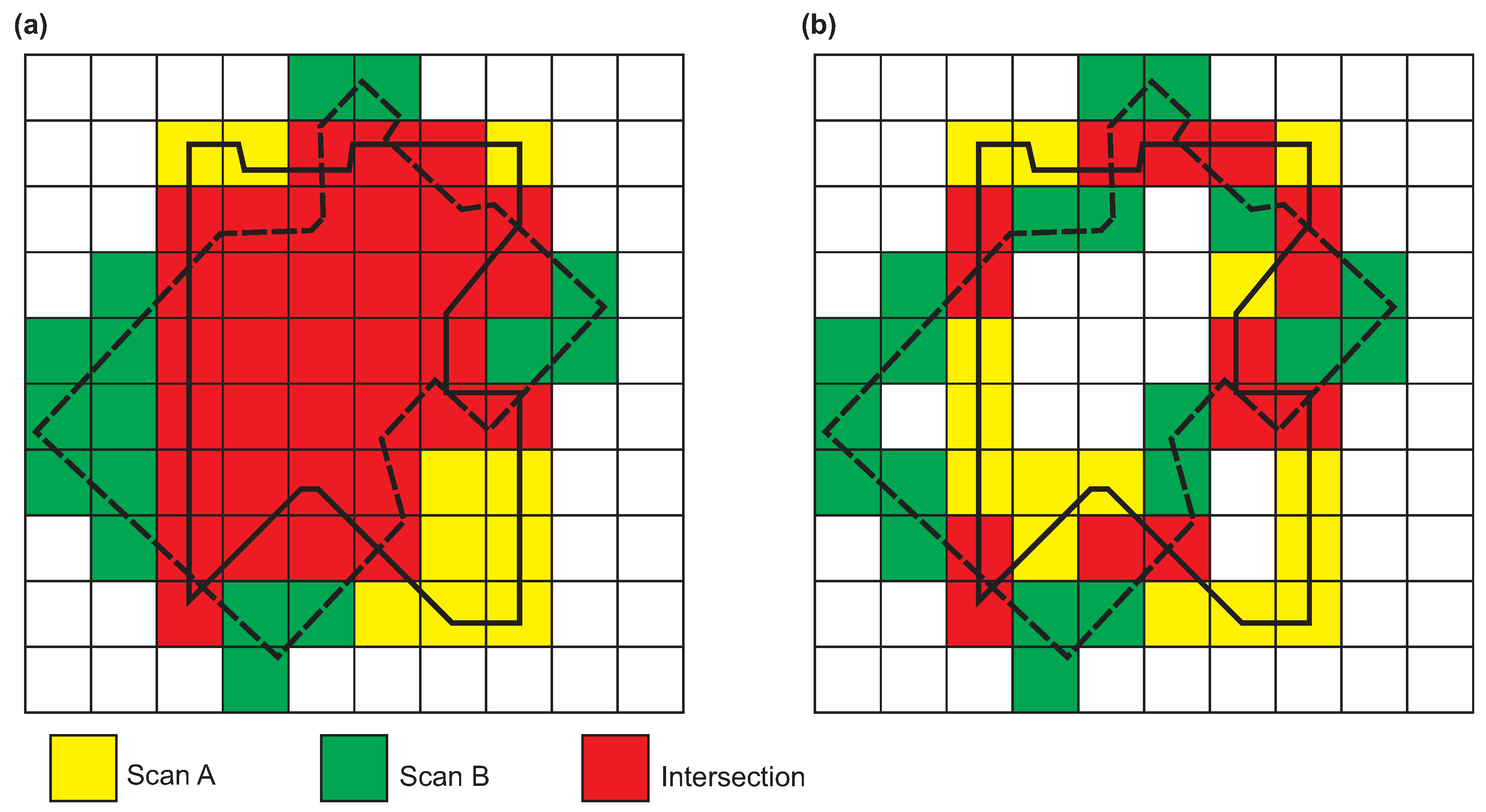
In the proposed approach, the laser range scan is converted to Cartesian coordinates in the same manner as in [44]. Next, a grid map simplifying the scene is created from the point cloud data. The grid map can be build using an arbitrary computationally feasible procedure. Figure 3 illustrates two methods for grid map creation. The approach, shown in Figure 3a, is based on area comparison. It assumes that the best scan match is achieved when the total volume of the overlapping regions is maximized. For each cell in the grid, the algorithm decides whether it is inside of the first or the second scan and then computes the number of overlapping cells. The second method, shown in Figure 3b, is based on boundary line analysis. It assumes that the best scan match is obtained when the intersection of the boundary lines is maximized. This approach does not require any operations over empty grid cells and laser scans can be represented by lists of non-empty grid cells that contain the points of the scans.

During the grid map creation, more than one point can be located in a single grid cell. This fact can be used by the scan matching procedure. For example, each cell can have a weight corresponding to the number of points it contains [42]. The cell weight can then affect the remainder of the scan matching procedure. However, initial experiments carried out in the scope of this study showed that the use of cell weights leads to the premature convergence of the optimization process and, in many cases, it prevents the algorithm from reaching the global optima. The scan matching algorithm is more robust when the cell weights are not taken into account and the grid cells are simply marked as occupied or empty. The number of occupied cells is usually not greater than 10% of all grid cells and the creation of grid maps as well as their comparison is fast.

3.5. Differential Evolution

Differential evolution (DE) is a successful stochastic evolutionary optimization method for continuous parameter optimization [55,56]. It is an evolutionary optimization process based on the concept of scaled vector differentials. The DE represents a continuous alternative to the widespread genetic algorithms that work with a discrete encoding of the candidate solutions. Both algorithms are nature-inspired problem-solving strategies that evolve a population of candidate solutions. On the other hand, they use different solution encodings (real–valued vs. discrete one), apply different operations to evolve the population and as a result implement different search strategies.

The DE algorithm has a history of successful applications in many industrial and engineering domains. It was designed as a generic global optimization metaheuristic but with practical engineering applications in mind [56]. It was used, among others, to predict the ground state structures of hydrogenated amorphous silicon (Si-H) clusters in material science, to streamline non-imaging optical design in optics and lightning development, to achieve 3D image registration in healthcare imaging, to design transversal digital filters in electronics and in particular signal processing, to fuse sensor data in robotics , to optimize industrial compressor supply systems, to realize system identification for decision making and in general in the area of robotics and expert systems [56]. The algorithm has also been applied in electrical engineering and electromagnetics. For example, it was used to optimize design of antennas for low signal-to-noise ratio conditions, to improve power allocation for the interleave-division multiple-access channel access method, to optimize antenna locations in a wireless network for maximum space coverage and to optimize source pulses and detection template in ultra-wideband radio systems. In the area of electromagnetics, the DE has been used to solve electromagnetic inverse scattering problems, the frequency assignment problem with real-world constraints and multiple objectives and to model large devices with distributed dipoles [56].

The wide variety of industrial applications shows that the DE is a metaheuristic optimization algorithm popular among practitioners. In this article, it is used as an optimization method for the registration of two 2-dimensional laser range scans.

From an optimization point of view, the DE evolves a group (population) of real-valued vectors by an iterative application of the differential mutation and crossover operations [55]. So-called trial vectors are in every iteration of the algorithm created from the current population by the differential mutation and recombined with corresponding target vectors by the crossover operator. The novel solutions the trial vectors represent are evaluated in the context of the problem and the trial vectors compete with the target vectors for survival in the population.

The DE procedure starts with a randomly constructed population of N real–valued vectors. In the course of the evolution, new trial vectors are created as scaled perturbations of existing population vectors. The algorithm creates trial vectors as scaled differences of a minimum of two distinct population vectors added to a third one. If a trial vector represents a better solution than the corresponding target vector, it takes its place in the population.

DE’s most important control parameters are scaling factor and mutation probability [55]. The scaling factor, $F\in [0,\infty ]$, affects the rate at which the population evolves and the crossover probability, $C\in [0,1]$, regulates the ratio of elements (vector values) that are transferred to the trial vector from the target vector. Population size, N and the choice of particular differential operators are important parameters of the top–level optimization process, too.

The elementary DE operations can be defined using the following equations [55]: the random initialization of the ith vector of length N is given by

$$\begin{array}{cc}\hfill {\overrightarrow{x}}_i\left[j\right]& =\mathrm{rand}(b_j^{\mathrm{L}},b_j^{\mathrm{U}}),j\in \{1,\dots ,N\},\hfill \end{array}$$

(9)

where $b_j^{\mathrm{L}}$ is the lower bound of the j-th parameter, $b_j^{\mathrm{U}}$ is the upper bound of the j-th parameter and $\mathrm{rand}(a,b)$ returns a random number from the range $[a,b]$. The basic differential mutation is defined as

$$\begin{array}{cc}\hfill {\overrightarrow{v}}_i& ={\overrightarrow{v}}_{r1}+F({\overrightarrow{v}}_{r2}-{\overrightarrow{v}}_{r3}),\hfill \end{array}$$

(10)

where F is the scaling factor and ${\overrightarrow{v}}_{r1}$, ${\overrightarrow{v}}_{r2}$ and ${\overrightarrow{v}}_{r3}$ are three distinct vectors selected randomly from the population. The vector ${\overrightarrow{v}}_{r1}$ is the base vector, ${\overrightarrow{v}}_{r2}$ and ${\overrightarrow{v}}_{r3}$ are the difference vectors and ${\overrightarrow{v}}_i$ is the trial vector.

The uniform (binomial) crossover that combines the target vector, ${\overrightarrow{x}}_i$, with the trial vector, ${\overrightarrow{v}}_i$, is given by

$$\begin{array}{cc}\hfill v_i\left[j\right]& =\left\{\begin{array}{cc}{v}_i\left[j\right]\hfill & if(\mathrm{rand}(0,1)<C) \mathrm{or} j=j_{\mathrm{rand}}\hfill \\ x_i\left[j\right],\hfill & \mathrm{otherwise}\hfill \end{array}\right.\hfill \end{array}$$

(11)

for each $j\in \{1,\dots ,N\}$. The index $j_{\mathrm{rand}}$ is selected at random as $j_{\mathrm{rand}}=\mathrm{rand}(1,N)$. The operator swaps the parameters in ${\overrightarrow{v}}_i$ with the parameters in ${\overrightarrow{x}}_i$ with probability equal to $1-C$. The outline of the classic DE according to [55] is summarized in Algorithm 1.

Algorithm 1: A summary of the basic DE.

4. Scan Matching by Cross-Correlation and Differential Evolution

A novel mobile robot self-localization strategy that uses the combination of cross-correlation of laser range scans [42] and the DE is designed and evaluated in this work. It improves a recent DE-based scan matching algorithm [44] through the use of laser range scan cross-correlation as an accurate and computationally lightweight fitness function. In this approach, the DE is used as an optimization mechanism to find the optimal set of parameters for an affine transformation that aligns two 2-dimensional laser range scans so that their mutual cross-correlation is maximized. The parameters of the transformation correspond to the displacement of a mobile robot in the direction of the x and y axes, $t_x$ and $t_y$ and its rotation, $\mathsf{\Phi }$. The algorithm evolves a population of 3-dimensional candidate transformation vectors, $\overrightarrow{t}=(t_x,t_y,\mathsf{\Phi })$.

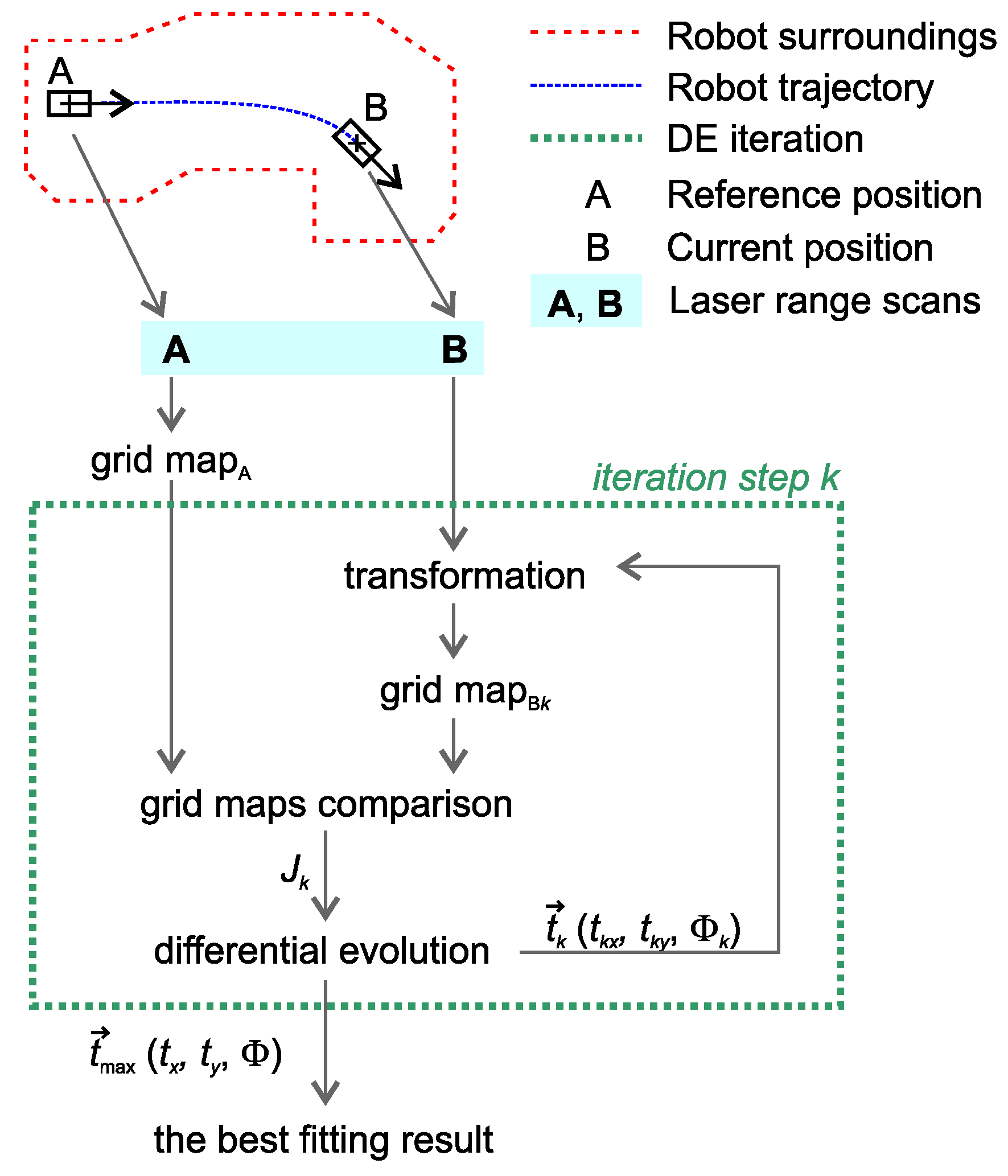
A graphical outline of the proposed scan matching process is shown in Figure 4. The figure shows a mobile robot moving in an indoor environment. On its way, the robot moved from a point of reference, A, to its current position, B. At each location, it acquired laser range scans denoted as $\mathbf{A}$ and $\mathbf{B}$, respectively. Each laser range scan produces a 2-dimensional point cloud in polar coordinates that represents the surroundings of the robot in the field-of-view of the LiDAR. The first scan, $\mathbf{A}$, is transformed into a grid map, map${}_{\mathrm{A}}$, by Algorithm 2, to represent the original position of the robot.

Algorithm 2: Pseudocode of grid map composition.

The second scan, $\mathbf{B}$, is matched with $\mathbf{A}$ by the DE algorithm. In each step, k, of every generation of DE, scan $\mathbf{B}$ is transformed by $\mathcal{T}$ with parameter vector, ${\overrightarrow{t}}_k=\left(t_x,t_y,\mathsf{\Phi }\right)$, encoded by the k-th trial vector. Grid map map${}_{\mathrm{Bk}}$ is then created from $\mathbf{B}k$ and the cross-correlation of map${}_{\mathrm{A}}$ and map${}_{\mathrm{Bk}}$ is evaluated using Algorithm 3. The resulting degree of alignment,

$$J(\mathbf{A},\mathbf{B},{\overrightarrow{t}}_k)=\mathrm{CC}\left[\mathrm{GM}\left(\mathbf{A}\right),\mathrm{GM}\left(\mathcal{T}\left(\mathbf{B},t_{kx},t_{ky},{\mathsf{\Phi }}_k\right)\right)\right],$$

(12)

is taken by the DE as a fitness function. The fitness function consists of cross-correlation, CC, which is basically the implementation of ⊙ (see Equation (8)) and the function which creates grid map from a scan, GM. It determines whether the trial vector substitutes the corresponding target vector in the population. This procedure is iteratively repeated until the DE terminates. The best solution found by the DE corresponds to the best set of parameters and defines the transformation leading to the maximum cross-correlation between grid mas map${}_{\mathrm{A}}$ and map${}_{\mathrm{Bk}}$.

Algorithm 3: Pseudocode of cross-correlation.

5. Experimental Evaluation

A variety of computer experiments were carried out to evaluate the ability of DE with cross-correlation as fitness function to perform point-based laser scan matching for self-localization of an autonomous mobile robot. The experiments used a series of simulated laser scans of an indoor environment describing the sensor readings of a virtual mobile robot moving through a room. The location data, corresponding to the simulated robot trajectory, was used as the ground truth.

5.1. Simulation Framework and Experimental Data

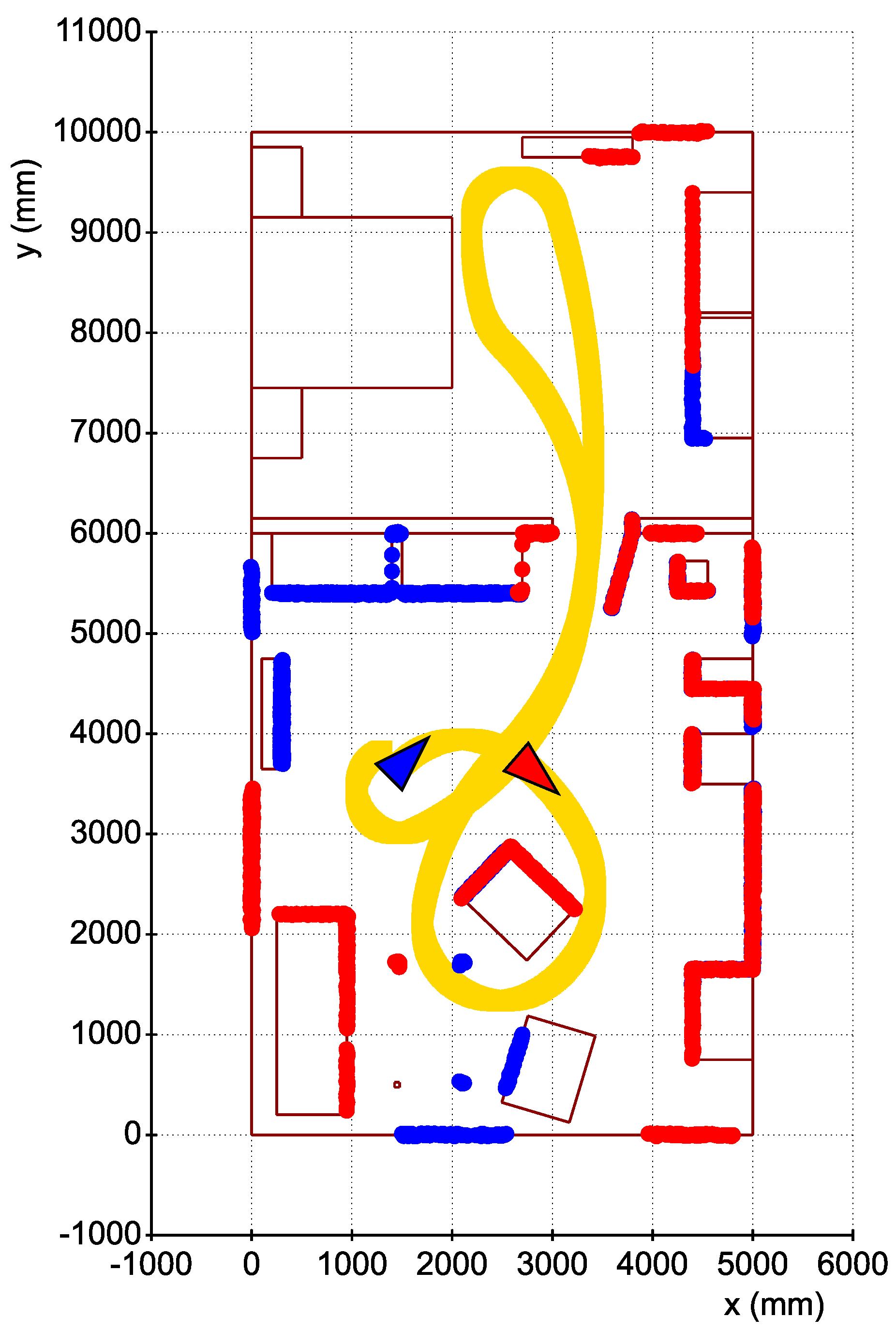
The software framework, introduced in [45], allows the simulation of a mobile robot in an indoor environment. It provides data corresponding to the laser scans performed by a common type of LiDAR, SICK LMS 100, mounted on top of a mobile robot. The robot moves through a surroundings with topology and obstacles defined by a map (stored in an XML configuration file). The framework provides data of the laser scans, robot’s absolute position and orientation assumed by the robot on its way. The data is stored in a CSV file with each line corresponding to one laser range scan. Figure 5 displays an example of a map in the simulation framework with the simulated robot trajectory (yellow) and two simulated laser scans (red, blue) highlighted.

5.2. Experimental Methodology

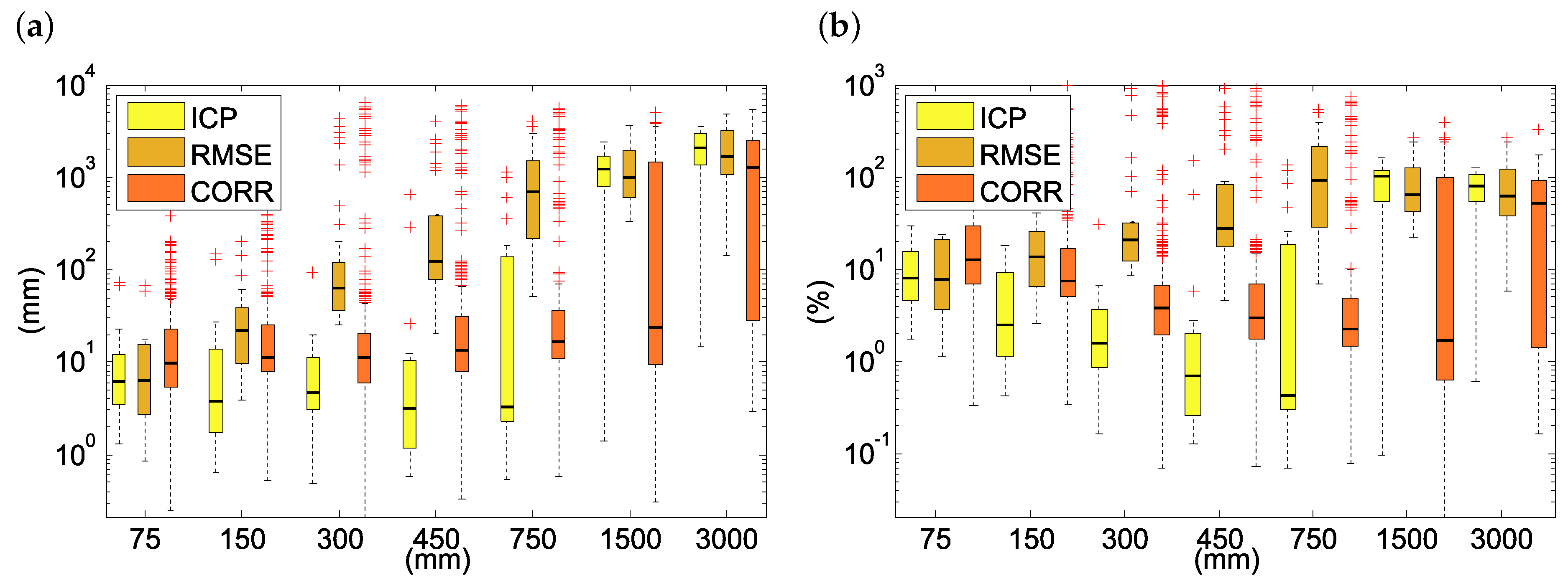
In each experiment, the DE was used to search for parameters of transformation $\mathcal{T}$ that would align selected pairs of laser scans from the data set created using the simulation framework. 20 random laser range scans were selected from a single robot trajectory and matched with subsequent scans taken 5, 10, 20, 30, 50, 100 and 200 LiDAR cycles later. That roughly corresponded to traveled distances of 75, 150, 300, 450, 750, 1500 and 3000 mm. In total, 140 distinct scans were matched during the experiments.

The experiments used the traditional/DE/rand/1 variant of the differential evolution with cross-correlation defined according to Section 3.4 as the fitness function. The DE worked with a population of 3-dimensional vectors representing the transformation parameters, $t_x,t_y$ and $\mathsf{\Phi }$. The remaining DE parameters were set after a series of trial-and-error runs and with respect to best practices and past experience. The size of the population, M, was set to 100, the crossover probability, C and the scaling factor, F, were both set to 0.9. The evolution was terminated after the maximum of 5000 generations and all experiments were independently executed 50 times to avoid bias caused the stochastic nature of the algorithm.

6. Results

In this section, the results of the computational experiments are detailed and the proposed evolutionary scan matching strategy based on cross-correlation (denoted CORR) is compared with a recent approach based on root mean square error (denoted RMSE) [44] and with the standard ICP algorithm [52].

Table 2. The translation and rotation errors of scan matching by the ICP, RMSE and CORR  methods.

Per-	Absolute Translation Error			Relative Translation Error			Absolute Rotation Error			Relative Rotation Error
Cen-	(mm)			(%)			(${}^{\circ }$)			(%)
tile	ICP	RMSE	CORR	ICP	RMSE	CORR	ICP	RMSE	CORR	ICP	RMSE	CORR
75 mm
25th	3.5	2.7	5.4	4.6	3.6	7.0	0.18	0.02	0.08	11.0	2.1	2.8
50th	6.1	6.4	9.7	8.1	7.8	12.7	0.40	0.08	0.19	15.0	5.2	11.9
75th	11.9	15.7	22.5	15.9	20.9	30.0	0.78	0.26	0.36	49.0	14.0	38.4
150 mm
25th	1.7	9.9	7.9	1.2	6.6	5.1	0.11	0.12	0.09	2.5	6.7	1.7
50th	3.8	22.2	11.4	2.5	13.6	7.5	0.25	0.40	0.17	4.9	12.1	5.1
75th	13.8	38.4	25.4	9.2	25.6	16.9	0.64	1.27	0.36	21.6	21.0	15.8
300 mm
25th	3.0	36.5	5.9	0.9	12.2	2.0	0.08	0.48	0.07	0.5	11.9	1.0
50th	4.7	62.6	11.3	1.6	21.0	3.8	0.25	1.14	0.17	4.1	17.9	2.4
75th	11.1	120.5	20.5	3.7	32.0	6.6	0.49	5.50	0.37	9.5	42.8	5.3
450 mm
25th	1.2	77.1	7.8	0.3	17.2	1.7	0.03	1.03	0.10	0.2	14.1	0.9
50th	3.2	124.3	13.2	0.7	28.0	2.9	0.07	2.31	0.25	0.9	29.8	1.8
75th	10.4	376.2	31.4	2.0	83.7	7.0	0.43	9.37	0.44	3.0	95.7	6.4
750 mm
25th	2.3	215.0	11.0	0.3	28.7	1.5	0.05	5.12	0.09	0.3	34.7	0.5
50th	3.2	704.8	16.8	0.4	91.6	2.3	0.12	13.64	0.19	0.8	55.9	1.1
75th	135.9	1535.0	36.3	18.6	212.7	4.9	1.12	88.81	0.45	10.5	270.6	2.8
1500 mm
25th	814.7	615.4	9.5	55.1	41.5	0.6	26.66	13.04	0.15	71.1	58.3	0.5
50th	1212.9	975.1	23.5	100.8	65.1	1.7	81.03	37.67	0.53	127.1	111.5	1.7
75th	1709.7	1915.8	1479.4	115.9	127.4	98.8	128.64	117.91	90.90	369.2	275.8	88.5
3000 mm
25th	1382.2	1076.6	27.7	54.4	37.5	1.4	43.72	77.87	0.93	72.9	90.5	1.1
50th	2084.5	1700.7	1257.6	81.2	61.9	52.6	92.49	151.26	93.41	111.0	144.5	106.4
75th	2948.9	3129.6	2466.5	106.3	121.2	91.0	163.38	167.56	167.99	229.4	518.3	365.4
Total
25th	2.8	30.2	8.2	1.0	14.8	1.8	0.10	0.45	0.10	1.1	9.6	1.0
50th	8.9	141.5	15.6	5.1	31.0	5.3	0.49	2.57	0.25	9.6	28.4	2.8
75th	814.7	1076.6	51.6	69.1	91.1	18.0	26.07	51.61	1.17	85.9	113.4	19.7

provides the results of the comparison between the ICP, RMSE and CORR scan matching strategies. The table is divided into 8 sections. Each of the first 7 sections summarizes the relative and absolute translation and rotation errors of all scan matching cases for scans taken after the robot traveled 75, 150, 300, 450, 750, 1500 and 3000 mm, respectively. The 8th section provides a summary of the errors for all scan matching experiments. The absolute translation error is the euclidean distance between the true ($l_{\mathrm{true}}$) and the estimated ($l_{\mathrm{est}}$) location of the robot. The relative translation error (in percent) is defined as

$${\delta }_l=\frac{\left|l_{\mathrm{true}}-l_{\mathrm{est}}\right|}{l_{\mathrm{true}}}·100.$$

(13)

The absolute rotation error is calculated as the difference between the true (${\mathsf{\Phi }}_{\mathrm{true}}$) and the estimated (${\mathsf{\Phi }}_{\mathrm{est}}$) rotation of the robot and its relative form (in percent) is defined as

$${\delta }_{\mathsf{\Phi }}=\frac{\left|{\mathsf{\Phi }}_{\mathrm{true}}-{\mathsf{\Phi }}_{\mathrm{calc}}\right|}{{\mathsf{\Phi }}_{\mathrm{true}}}·100.$$

(14)

The percentile values corresponding to the 25th, 50th and the 75th percentile (i.e., the lower quartile, median and the upper quartile) of the errors for each algorithm are shown in the individual sections of Table 2. The lower the percentile value, the better the results and thus the algorithm performance.

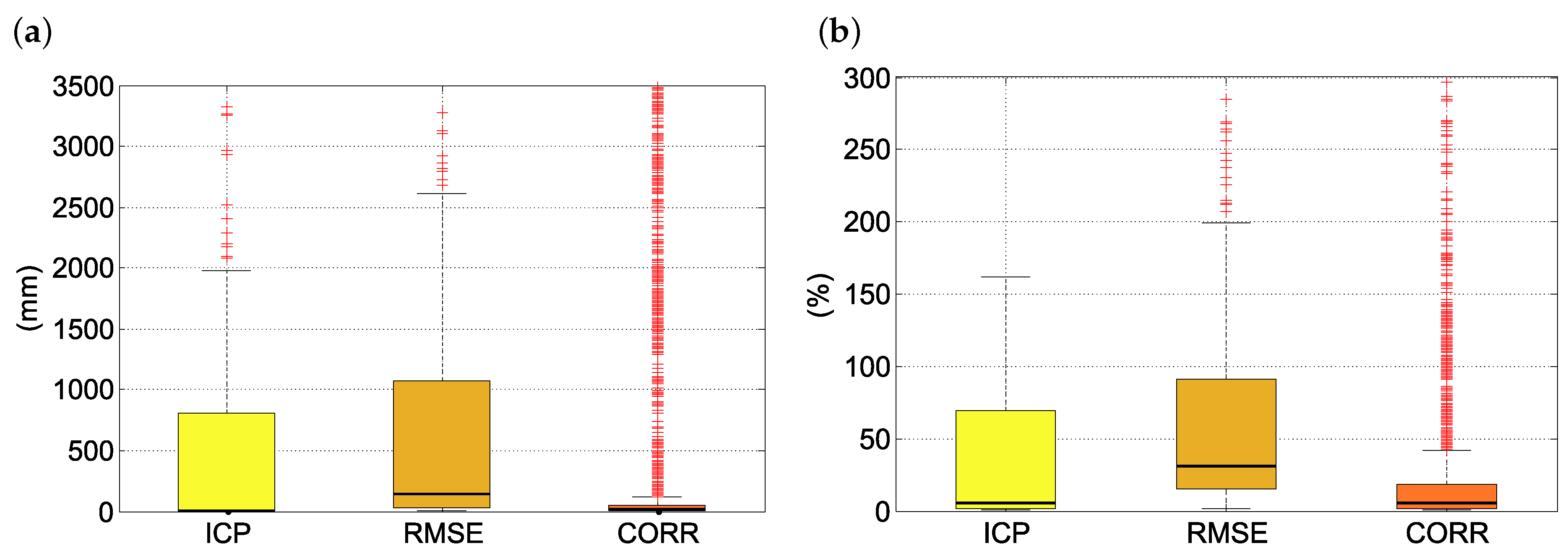
Figure 6 illustrates the distribution of the absolute and the relative translation errors of all scan matching experiments performed with the ICP, RMS and CORR algorithms. Results shown in Figure 6b indicate that the difference between the medians of the relative translation errors of the standard ICP and the proposed CORR algorithm is not significant (5.1% ICP, 5.3% CORR). This can be attributed to the uniformly distributed noise generated by the simulation framework used for the experiments [45]. Furthermore, the CORR method has significantly lower translation error values at the lower and upper quartiles than the other tested methods. This shows that the proposed algorithm achieves for the majority of the considered test cases a robust and accurate scan matching functionality. In general, the RMSE method obtains scan matching with a higher error than the other two methods.

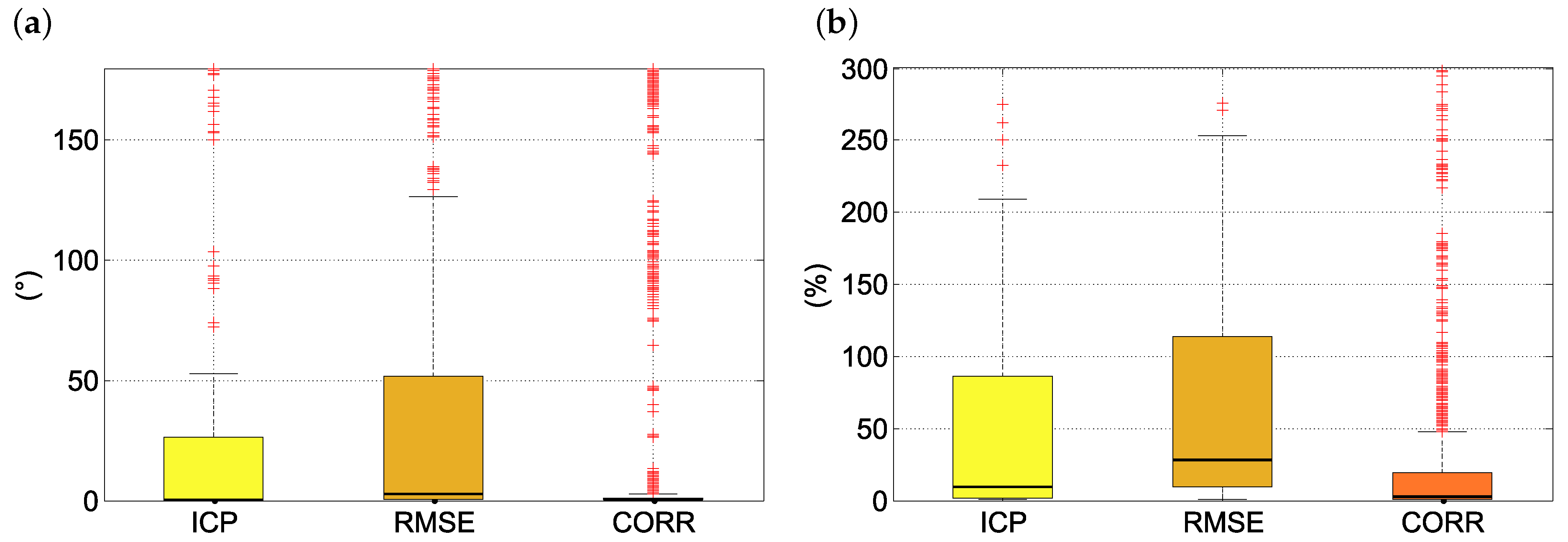
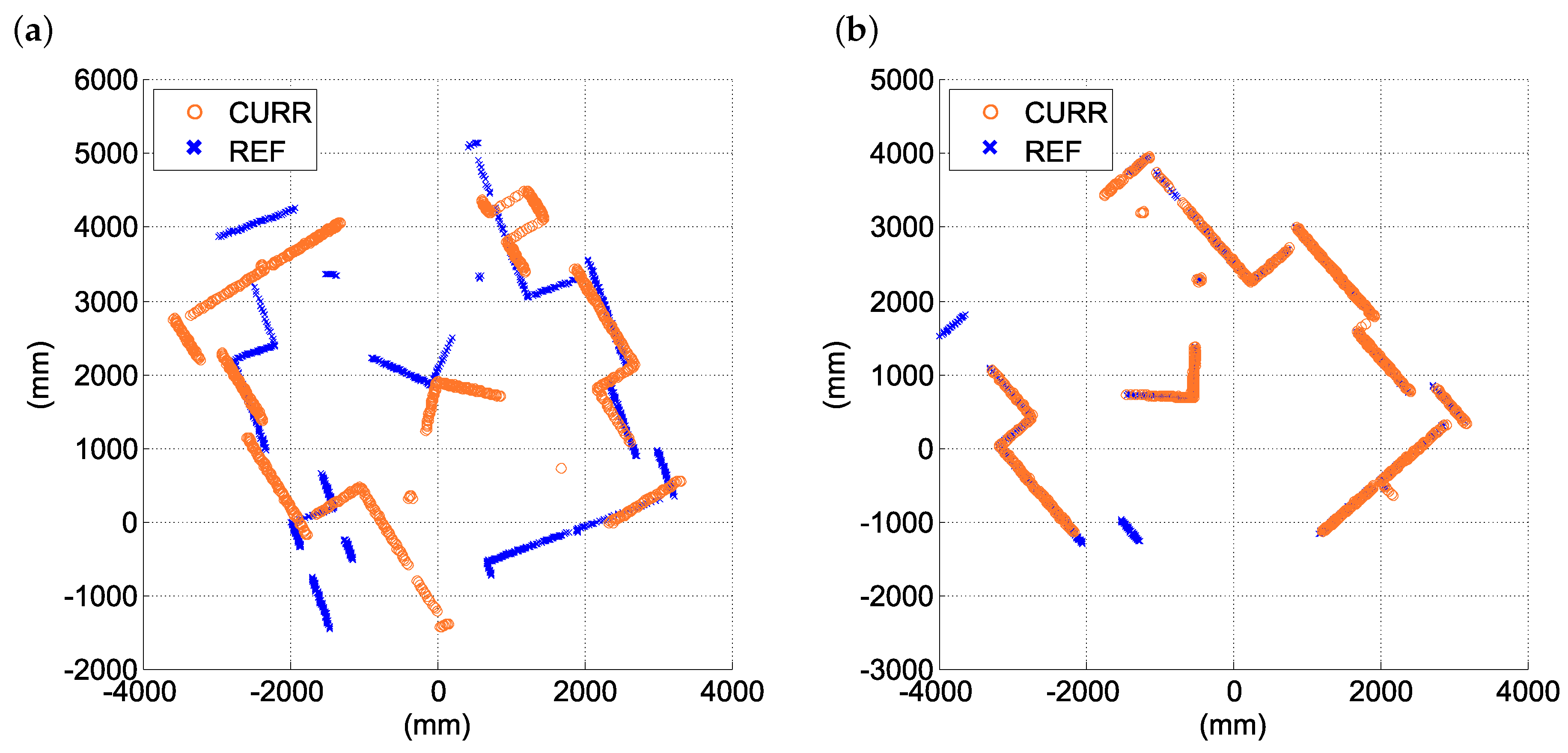
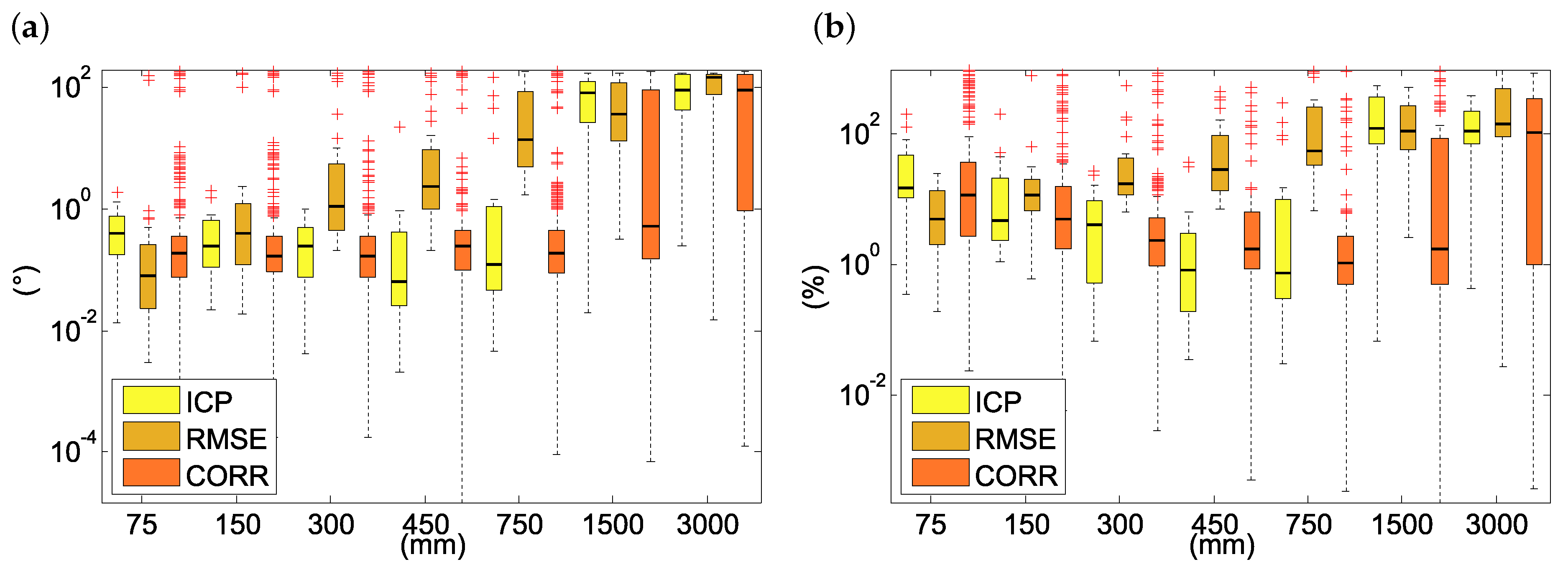
The absolute and the relative rotation errors of all scan matching experiments are shown in Figure 7. The box plots clearly demonstrate that the proposed CORR algorithm achieves better (i.e., lower) error values for all observed translation error percentiles. The median relative error value of the CORR method is 2.8% while the standard ICP algorithm has relative error of 9.6%. Similarly to its performance on translation, the RMSE method performs the worst of the three compared scan matching strategies with median relative rotation error of 28.4% . Figure 7a also reveals some important information about the nature of rotation errors of the ICP and CORR methods. The rotation outliers, that is, scan matching cases with high absolute rotation error, are concentrated in the proximity of 90${}^{\circ }$ and 180${}^{\circ }$ values. The false alignments are caused by the tendency of both algorithms to converge to local rotation optima which is typically situated around 90${}^{\circ }$, 180${}^{\circ }$ and 270${}^{\circ }$. This situation is illustrated in the following pair of figures. Figure 8a shows a wrong alignment at a local rotation optimum of 180${}^{\circ }$, while Figure 8b shows the correct alignment. The relatively high number of rotation outliers in results obtained by the CORR method indicate its higher sensitivity to rotation errors, compared to the ICP algorithm.

Comparisons of translation and rotation errors of scan matching experiments in relation to the length of the robot trajectory between the scans are shown, respectively, in Figure 9 and Figure 10. It can be seen that the ICP algorithm provides the best alignment for scans taken after the robot traveled between 75 mm to 450 mm. The error of scan alignment by ICP starts to rise for scans taken after the robot traveled 750 mm or more. Its accuracy deteriorates even more when matching laser range scans taken after the robot traveled long distances, that is, 1500 mm or 3000 mm. Based on the executed scan matching experiments, the proposed scan matching method (CORR) has for scans spaced 75 mm to 450 mm only slightly worse results than the ICP, still sufficient for practical indoor localization. However, the CORR algorithm shows superior results when matching laser range scans taken after the robot traveled long distances of 750 mm or more. In these cases, it provides significantly better localization than the standard ICP algorithm.

Figure 9 and Figure 10 also illustrate the convergence of the proposed approach. In contrast to the ICP, RMSE and CORR are both stochastic methods with random initialization. They were outperformed by the ICP for scans taken when the robot traveled between 75 and 750 mm in terms of minimum and average absolute and translation and rotation errors. However, the figures also clearly illustrate that all independent CORR runs that processed laser range scans taken after the robot moved 1500 mm and more obtained better average results than the ICP method. This suggests that the proposed approach, although not deterministic, produced in these cases, on average, scan alignments of better quality than the ICP method.

7. Conclusions

A novel scan matching strategy, based on the combination of cross-correlation and differential evolution, was introduced in this work. It uses cross-correlation as an accurate, robust and computationally efficient measure of the similarity of 2-dimensional laser range scans and differential evolution for the search of scan transformation parameters. The proposed scan matching strategy was implemented and extensively evaluated. The evaluation used a software framework for the simulation of the movement of an autonomous mobile robot in an interior. The framework generated a data set composed of virtual laser range scans, taken when the robot followed a pre-defined trajectory in a virtual room.

The proposed method was used to match laser range scans taken by the robot after it traveled different distances ranging from 75 mm to 3000 mm. The accuracy of the estimated translation and rotation of the robot was compared to the accuracy of translation and rotation obtained by a standard scan matching algorithm, ICP and a previous method based on a combination of RMSE and differential evolution. The experiments showed that the proposed method has only slightly lower accuracy than the ICP algorithm when matching laser range scans taken after the robot traveled between 75 mm and 750 mm but it achieved substantially better results for scans taken after it traveled 1500 mm or 3000 mm. The results of the computational experiments suggest that the proposed approach is an accurate and robust scan matching strategy suitable in particular for situations when the mobile robot travels longer distances.

The future work will include an efficient implementation of the proposed method for embedded devices (for example, NVIDIA Jetson Nano) and field tests with a physical mobile robot in a real environment.

References

- Turgut, Z.; Aydin, G.Z.G.; Sertbas, A. Indoor Localization Techniques for Smart Building Environment. Procedia Comput. Sci. 2016, 83, 1176–1181. [Google Scholar] [CrossRef] [Green Version]
- Zafari, F.; Gkelias, A.; Leung, K.K. A Survey of Indoor Localization Systems and Technologies. arXiv 2017, arXiv:1709.01015. [Google Scholar] [CrossRef]
- Syberfeldt, A.; Ayani, M.; Holm, M.; Wang, L.; Lindgren-Brewster, R. Localizing operators in the smart factory: A review of existing techniques and systems. In Proceedings of the 2016 International Symposium on Flexible Automation (ISFA), Cleveland, OH, USA, 1–3 August 2016; pp. 179–185. [Google Scholar] [CrossRef]
- Li, J.; Bao, J.; Yu, Y. Study on the Localization for a Rescue Robot Based on Laser Scan Matching. In Proceedings of the 2010 International Conference on Machine Vision and Human-Machine Interface, Kaifeng, China, 24–25 April 2010; pp. 642–645. [Google Scholar] [CrossRef]
- Cui, Y.A.; Cai, Z.X.; Lu, W.A. Scene recognition for mine rescue robot localization based on vision. Trans. Nonferrous Met. Soc. China 2008, 18, 432–437. [Google Scholar] [CrossRef]
- Wang, F.; Cui, J.Q.; Chen, B.M.; Lee, T. A comprehensive UAV indoor navigation system based on vision optical flow and laser FastSLAM. Zidonghua Xuebao/Acta Autom. Sin. 2013, 39, 1889–1900. [Google Scholar] [CrossRef]
- Bonaccorso, F.; Catania, F.; Muscato, G. Evaluation of Algorithms for indoor mobile robot self-localization through laser range finders data. In Proceedings of the 7th IFAC Symposium on Intelligent Autonomous Vehicles, Lecce, Italy, 6–8 September 2010; Volume 43, pp. 563–568. [Google Scholar]
- Sobreira, H.; Costa, C.M.; Sousa, I.; Rocha, L.; Lima, J.; Farias, P.C.M.A.; Costa, P.; Moreira, A.P. Map-Matching Algorithms for Robot Self-Localization: A Comparison Between Perfect Match, Iterative Closest Point and Normal Distributions Transform. J. Intell. Robot. Syst. 2018. [Google Scholar] [CrossRef]
- Kaboli, A.; Bowling, M.; Musilek, P. Bayesian Calibration for Monte Carlo Localization. In Proceedings of the 21st Conference on Artificial Intelligence (AAAI-06), Boston, MA, USA, 16–20 July 2006; pp. 964–969. [Google Scholar]
- Gu, Y.; Lo, A.; Niemegeers, I. A survey of indoor positioning systems for wireless personal networks. IEEE Commun. Surv. Tutor. 2009, 11, 13–32. [Google Scholar] [CrossRef] [Green Version]
- Mainetti, L.; Patrono, L.; Sergi, I. A survey on indoor positioning systems. In Proceedings of the 2014 22nd International Conference on Software, Telecommunications and Computer Networks (SoftCOM), Split, Croatia, 17–19 September 2014; pp. 111–120. [Google Scholar] [CrossRef]
- Guanlao, R.; Musilek, P.; Ahmad, F.; Kaboli, A. Fuzzy situation based navigation of autonomous mobile robot using reinforcement learning. In Proceedings of the Annual Meeting of the North American Fuzzy Information Processing Society (NAFIPS’04), Banff, AB, Canada, 27–30 June 2004; pp. 820–825. [Google Scholar]
- Filliat, D.; Meyer, J.A. Map-based navigation in mobile robots: I. A review of localization strategies. Cogn. Syst. Res. 2003, 4, 243–282. [Google Scholar] [CrossRef]
- Karahan, M.; Erkmen, A.; Erkmen, I. Prioritized Mobile Robot Exploration Based on Percolation Enhanced Entropy Based Fast SLAM. J. Intell. Robot. Syst. Theory Appl. 2013, 75, 541–567. [Google Scholar] [CrossRef]
- Dumble, S.; Gibbens, P. Efficient Terrain-Aided Visual Horizon Based Attitude Estimation and Localization. J. Intell. Robot. Syst. 2015, 78, 205–221. [Google Scholar] [CrossRef]
- Bosse, M.; Zlot, R. Map matching and data association for large-scale two-dimensional laser scan-based SLAM. Int. J. Robot. Res. 2008, 27, 667–691. [Google Scholar] [CrossRef]
- Corso, N.; Zakhor, A. Indoor localization algorithms for an ambulatory human operated 3D mobile mapping system. Remote Sens. 2013, 5, 6611–6646. [Google Scholar] [CrossRef]
- Hornung, A.; Oßwald, S.; Maier, D.; Bennewitz, M. Monte carlo localization for humanoid robot navigation in complex indoor environments. Int. J. Humanoid Robot. 2014, 11, 1441002. [Google Scholar] [CrossRef]
- Kurecka, A.; Konecny, J.; Prauzek, M.; Koziorek, J. Monte carlo based wireless node localization. Elektron. Ir Elektrotech. 2014, 20, 12–16. [Google Scholar] [CrossRef]
- Jiang, Z.; Zhou, W.; Li, H.; Mo, Y.; Ni, W.; Huang, Q. A New Kind of Accurate Calibration Method for Robotic Kinematic Parameters Based on the Extended Kalman and Particle Filter Algorithm. IEEE Trans. Ind. Electron. 2018, 65, 3337–3345. [Google Scholar] [CrossRef]
- Dellaert, F.; Fox, D.; Burgard, W.; Thrun, S. Monte Carlo localization for mobile robots. Proc. IEEE Int. Conf. Robot. Autom. 1999, 2, 1322–1328. [Google Scholar]
- Weikersdorfer, D.; Adrian, D.B.; Cremers, D.; Conradt, J. Event-based 3D SLAM with a depth-augmented dynamic vision sensor. In Proceedings of the IEEE International Conference on Robotics and Automation, Hong Kong, China, 31 May–7 June 2014; pp. 359–364. [Google Scholar]
- Chen, Y.; Tang, J.; Jiang, C.; Zhu, L.; Lehtomäki, M.; Kaartinen, H.; Kaijaluoto, R.; Wang, Y.; Hyyppä, J.; Hyyppä, H.; et al. The accuracy comparison of three simultaneous localization and mapping (SLAM)-based indoor mapping technologies. Sensors 2018, 18, 3228. [Google Scholar] [CrossRef] [PubMed]
- Bardow, P.; Davison, A.J.; Leutenegger, S. Simultaneous optical flow and intensity estimation from an event camera. In Proceedings of the IEEE Computer Society Conference on Computer Vision and Pattern Recognition, Las Vegas, NV, USA, 27–30 June 2016; Volume 2016, pp. 884–892. [Google Scholar]
- Hermand, E.; Nguyen, T.; Hosseinzadeh, M.; Garone, E. Constrained Control of UAVs in Geofencing Applications. In Proceedings of the MED 2018 26th Mediterranean Conference on Control and Automation (MED), Zadar, Croatia, 19–22 June 2018; pp. 217–222. [Google Scholar]
- Ballesteros-Escamilla, M.; Cruz-Ortiz, D.; Chairez, I.; Luviano-Juárez, A. Adaptive output control of a mobile manipulator hanging from a quadcopter unmanned vehicle. ISA Trans. 2019. [Google Scholar] [CrossRef]
- Friedman, C.; Chopra, I.; Rand, O. Perimeter-Based Polar Scan Matching (PB-PSM) for 2D Laser Odometry. J. Intell. Robot. Syst. Theory Appl. 2015, 80, 231–254. [Google Scholar] [CrossRef]
- Park, S.; Park, S.K. Global localization for mobile robots using reference scan matching. Int. J. Control. Autom. Syst. 2014, 12, 156–168. [Google Scholar] [CrossRef]
- Gao, Y.; Liu, S.; Atia, M.; Noureldin, A. INS/GPS/LiDAR integrated navigation system for urban and indoor environments using hybrid scan matching algorithm. Sensors 2015, 15, 23286–23302. [Google Scholar] [CrossRef]
- Diosi, A.; Kleeman, L. Fast Laser Scan Matching using Polar Coordinates. Int. J. Robot. Res. 2007, 26, 1125–1153. [Google Scholar] [CrossRef]
- Rusinkiewicz, S.; Levoy, M. Efficient variants of the ICP algorithm. In Proceedings of the Third International Conference on 3-D Digital Imaging and Modeling, Québec City, QC, Canada, 28 May–1 June 2001; pp. 145–152. [Google Scholar]
- Teza, G.; Galgaro, A.; Zaltron, N.; Genevois, R. Terrestrial laser scanner to detect landslide displacement fields: A new approach. Int. J. Remote Sens. 2007, 28, 3425–3446. [Google Scholar] [CrossRef]
- Ishii, M.; Yokoyama, K. Mapping and correction method in static environments for autonomous mobile robot. Int. J. Soc. Mater. Eng. Resour. 2014, 20, 207–212. [Google Scholar] [CrossRef]
- Zezhong, X.; Jilin, L.; Zhiyu, X. Scan matching based on CLS relationships. In Proceedings of the IEEE International Conference on Robotics, Intelligent Systems and Signal Processing, Changsha, China, 8–13 October 2003; Volume 1, pp. 99–104. [Google Scholar]
- Weber, J.; Jörg, K.W.; von Puttkamer, E. APR—Global Scan Matching Using Anchor Point Relationships. In Proceedings of the Intelligent Autonomous Systems (IAS-6), Venice, Italy, 25–27 July 2000. [Google Scholar]
- Sun, Q.; Yuan, J.; Zhang, X.; Sun, F. RGB-D SLAM in Indoor Environments with STING-Based Plane Feature Extraction. IEEE/ASME Trans. Mechatron. 2018, 23, 1071–1082. [Google Scholar] [CrossRef]
- Li, J.; Zhong, R.; Hu, Q.; Ai, M. Feature-based laser scan matching and its application for indoor mapping. Sensors 2016, 16, 1265. [Google Scholar] [CrossRef]
- Prieto, P.G.; Martin, F.; Moreno, L.; Carballeira, J. DENDT: 3D-NDT scan matching with Differential Evolution. In Proceedings of the 2017 25th Mediterranean Conference on Control and Automation, MED 2017, Valletta, Malta, 3–6 July 2017; pp. 719–724. [Google Scholar]
- Biber, P.; Strasser, W. The normal distributions transform: A new approach to laser scan matching. In Proceedings of the 2003 IEEE/RSJ International Conference on Intelligent Robots and Systems (IROS 2003) (Cat. No.03CH37453), Las Vegas, NV, USA, 27–31 October 2003; Volume 3, pp. 2743–2748. [Google Scholar]
- Martin, F.; Triebel, R.; Moreno, L.; Siegwart, R. Two different tools for three-dimensional mapping: DE-based scan matching and feature-based loop detection. Robotica 2014, 32, 19–41. [Google Scholar] [CrossRef]
- Mirkhani, M.; Forsati, R.; Shahri, A.M.; Moayedikia, A. A novel efficient algorithm for mobile robot localization. Robot. Auton. Syst. 2013, 61, 920–931. [Google Scholar] [CrossRef]
- Konecny, J.; Prauzek, M.; Kromer, P.; Musilek, P. Novel Point-to-Point Scan Matching Algorithm Based on Cross-Correlation. Mob. Inf. Syst. 2016, 2016, 6463945. [Google Scholar] [CrossRef]
- Konecny, J.; Prauzek, M.; Hlavica, J. SLAM algorithm based on cross-correlation scan matching. In Proceedings of the 8th International Conference on Signal Processing Systems, Auckland, New Zealand, 21–24 November 2016; pp. 89–93. [Google Scholar]
- Kromer, P.; Konecny, J.; Prauzek, M. Point-based scan matching by differential evolution. In Proceedings of the 2016 International Conference on Intelligent Networking and Collaborative Systems, IEEE INCoS 2016, Ostrawva, Czech Republic, 7–9 September 2016; pp. 215–221. [Google Scholar]
- Konecny, J.; Prauzek, M.; Hlavica, J. Indoor LiDAR Scan Matching Simulation Framework for Intelligent Algorithms Evaluation. In Proceedings of the First International Scientific Conference “Intelligent Information Technologies for Industry” (IITI’16), Sochi, Russia, 16–21 May 2016; Advances in Intelligent Systems and Computing. Volume 451, pp. 355–364. [Google Scholar]
- Kotzian, J.; Konecny, J.; Prokop, H.; Lippa, T.; Kuruc, M. Autonomous explorative mobile robot: Navigation and construction. In Proceedings of the 9th RoEduNet IEEE International Conference, RoEduNet 2010, Sibiu, Romania, 24–26 June 2010; pp. 49–54. [Google Scholar]
- ARM Information Center. Available online: http://infocenter.arm.com (accessed on 15 July 2019).
- Wen, J.; Qian, C.; Tang, J.; Liu, H.; Ye, W.; Fan, X. 2D LiDAR SLAM Back-End Optimization with Control Network Constraint for Mobile Mapping. Sensors 2018, 18, 3668. [Google Scholar] [CrossRef]
- Wang, Z.; Chen, Y.; Mei, Y.; Yang, K.; Cai, B. IMU-Assisted 2D SLAM Method for Low-Texture and Dynamic Environments. Appl. Sci. 2018, 8, 2534. [Google Scholar] [CrossRef]
- Wang, W.; Sakurada, K.; Kawaguchi, N. Reflectance Intensity Assisted Automatic and Accurate Extrinsic Calibration of 3D LiDAR and Panoramic Camera Using a Printed Chessboard. Remote. Sens. 2017, 9, 851. [Google Scholar] [CrossRef]
- Besl, P.J.; McKay, N.D. A Method for Registration of 3-D Shapes. IEEE Trans. Pattern Anal. Mach. Intell. 1992, 14, 239–256. [Google Scholar] [CrossRef]
- Konecny, J.; Prauzek, M.; Hlavica, J. ICP Algorithm in Mobile Robot Navigation: Analysis of Computational Demands in Embedded Solutions. IFAC-PapersOnLine 2016, 49, 396–400. [Google Scholar] [CrossRef]
- Hazewinkel, M. Encyclopaedia of Mathematics: Monge—Ampère Equation—Rings and Algebras; Encyclopaedia of Mathematics; Springer: New York, NK, USA, 1995. [Google Scholar]
- Tan, C.C.; Hird, C.; Okada, Y. Processing of sound field signal of a constrained panel by cross-correlation. In Proceedings of the International Conference on Information, Communications and Signal Processing, ICICS, Singapore, 12 September 1997; Volume 1, pp. 316–320. [Google Scholar]
- Yang, X. Nature-Inspired Optimization Algorithms; Elsevier: Amsterdam, The Netherlands, 2014. [Google Scholar]
- Das, S.; Mullick, S.S.; Suganthan, P. Recent advances in differential evolution—An updated survey. Swarm Evol. Comput. 2016, 27, 1–30. [Google Scholar] [CrossRef]
Figure 1.
An outline of the simulation-based design.
Figure 2.
Scan matching: problem definition. (a) Scans before alignment (b) Scans after alignment.
Figure 3.
Degree of alignment approaches: (a) Area comparison (b) Boundary line comparison.
Figure 4.
Description of the proposed algorithm: laser range reading and DE-based scan matching.
Figure 5.
Simulation framework: an example of a map, robot trajectory (yellow) and two simulated laser scans (red, blue).
Figure 6.
A boxplot visualization of the absolute (a) and the relative (b) translation error of all scan matching experiments (section Total of Table 2).
Figure 7.
A boxplot visualization of the absolute (a) and the relative (b) rotation error of all scan matching experiments (section Total of Table 2).
Figure 8.
An example of scan alignment by the CORR method: (a) Incorrect alignment due to a rotation error. (b) Correct alignment.
Figure 9.
Absolute (a) and relative (b) translation errors of scan matching experiments for laser range scans taken after robot movement of 75–3000 mm.
Figure 10.
Absolute (a) and relative (b) rotation errors of scan matching experiments for laser range scans taken after robot movement of 75–3000 mm.