
Fuzzy Rough Nearest Neighbour Methods for Aspect-Based Sentiment Analysis


1
Computational Web Intelligence, Department of Applied Mathematics, Computer Science and Statistics, Ghent University, 9000 Ghent, Belgium
2
LT3 Language and Translation Technology Team, Ghent University, 9000 Ghent, Belgium
*
Author to whom correspondence should be addressed.
Electronics 2023, 12(5), 1088; https://doi.org/10.3390/electronics12051088
Submission received: 15 January 2023
/
Revised: 11 February 2023
/
Accepted: 20 February 2023
/
Published: 22 February 2023
(This article belongs to the Special Issue AI for Text Understanding)
Abstract
:Fine-grained sentiment analysis, known as Aspect-Based Sentiment Analysis (ABSA), establishes the polarity of a section of text concerning a particular aspect. Aspect, sentiment, and emotion categorisation are the three steps that make up the configuration of ABSA, which we looked into for the dataset of English reviews. In this work, due to the fuzzy nature of textual data, we investigated machine learning methods based on fuzzy rough sets, which we believe are more interpretable than complex state-of-the-art models. The novelty of this paper is the use of a pipeline that incorporates all three mentioned steps and applies Fuzzy-Rough Nearest Neighbour classification techniques with their extension based on ordered weighted average operators (FRNN-OWA), combined with text embeddings based on transformers. After some improvements in the pipeline’s stages, such as using two separate models for emotion detection, we obtain the correct results for the majority of test instances (up to 81.4%) for all three classification tasks. We consider three different options for the pipeline. In two of them, all three classification tasks are performed consecutively, reducing data at each step to retain only correct predictions, while the third option performs each step independently. This solution allows us to examine the prediction results after each step and spot certain patterns. We used it for an error analysis that enables us, for each test instance, to identify the neighbouring training samples and demonstrate that our methods can extract useful patterns from the data. Finally, we compare our results with another paper that performed the same ABSA classification for the Dutch version of the dataset and conclude that our results are in line with theirs or even slightly better.
1. Introduction
Since the advent of social media at the beginning of this century, the analysis of the wealth of user feedback written on these social platforms has become a vibrant research domain in the domain of natural language processing. While the classic sentiment analysis or opinion mining approaches mainly focused on determining the mood behind whole texts (review, letter, article, and other), more fine-grained approaches have also been proposed more recently, which give more insights into what exactly people like or dislike about a given product or service. In the case of the Aspect-Based Sentiment Analysis (ABSA), the task consists in determining the polarity of a part of the text describing a specific aspect of a given product or service [1].
For example, for the analysis of the following restaurant review: “The pizza was delicious, but the service was slow.”, we cannot use classical sentiment analysis to define the general sentiment of the customer, as it is neither wholly negative nor entirely positive. In this case, we can apply ABSA techniques, which will first determine what aspects of this restaurant visit are discussed (“pizza” and “service”); each of these aspect terms will then be assigned to an aspect category (e.g., FOOD_quality and SERVICE_speed), after which a sentiment label or even a more fine-grained emotion label will be assigned to each of these aspect categories (for example, “positive” and “negative” or “satisfaction” and “dissatisfaction”, correspondingly) [2].
This paper is one of the first attempts to apply fuzzy-rough-based methods to the ABSA three-level task. Previously, such techniques were already used for various other machine learning tasks, including in sentiment analysis and emotion detection. In particular, in [3,4,5], we investigated the application of fuzzy-rough methods for emotion categorisation, irony and hate speech detection. The datasets for these experiments originate from different SemEval competitions (https://semeval.github.io/, accessed on 14 January 2023). While the majority of the best-performing solutions submitted to these competitions were based on neural networks or transformers, our solutions achieved comparable results and were consistently ranked among the TOP-5 results, as demonstrated in [5]. At the same time, we were able to provide interpretability of our solution (as also demonstrated in Section 6), which is an important advantage when dealing with a subjective topic such as emotions. In the current work, we will demonstrate that this interpretable solution also obtains promising results for ABSA, predicting all three classes correctly for the majority of test instances.
The remainder of the paper has the following structure: Section 2 provides an overview of the most relevant studies about ABSA and our previous research. Section 3 gives a detailed overview of the task and data which with we will work. Section 4 is a methodological section, discussing data preprocessing, the embedding methods we explored and the structure of the pipelines we used. Section 5 discusses the results for the different experiments, while in Section 6, we provide an error analysis of those results with examples showcasing the explainability of our approach. Finally, Section 7 concludes our work and presents some thoughts regarding future work.
2. Related Work
In this section, we review the general ABSA task and explain how it evolved into its current form. We also discuss its use within SemEval competitions and introduce the specific task we are working with. Next, we provide an overview of interpretability types for text analysis models, and recall our own previous work on sentiment analysis using fuzzy-rough methods.
2.1. ABSA Studies Summary
One of the first studies that presented a task similar to ABSA was [6] in 2004, where the authors called this task “feature-based summary” or “feature-based opinion mining”. They formulated a sentiment analysis task that contains three subtasks: (1) identifying the specific product features about which customers left their opinion (referred to as product features), (2) identifying review sentences that give positive or negative opinions for each feature and (3) constructing a summary using the information that has been discovered.
Some years later, ref. [1] formulated ABSA as a task with two steps: aspect extraction and aspect sentiment classification. While initially, lexicon-based and feature-based supervised learning approaches were applied to the ABSA task, the introduction of transformer-based approaches in NLP also led to their application in ABSA. In [7], the authors presented a solution where a BERT-based architecture outperformed all previous approaches with a superficial linear classification layer. Later, in [8], the authors used adversarial training on a general BERT and a domain-specific post-trained BERT for the two ABSA tasks mentioned before: aspect extraction and aspect sentiment classification. Meanwhile, in [9], a knowledge-enabled language representation BERT-based model was introduced for the ABSA task. This model could provide explainable results by leveraging extra information obtained from a sentiment knowledge graph to navigate the input embedding of a sentence with a BERT language representation model.
Recent studies targeting ABSA are primarily based on transformer-based models [8,9,10]. Particularly, in [10], the authors presented a transformer-based multi-task learning framework. They called this solution the Cross-Modal Multitask Transformer, whose task is to deal with Multimodal Aspect-Based Sentiment Analysis (MABSA), where aspect-sentiment tandems were extracted from pairs of sentences and images.
ABSA was presented for the first time in the format of a shared task at SemEval 2014 Task 4 by [11]. The organisers presented several datasets of reviews for different business types, where aspect terms and their corresponding polarities were annotated for each sentence. They expanded their work in SemEval-2015 Task 12 [12], where all the recognised components of the expressed opinions (i.e., aspects, opinion target expressions, and sentiment polarities) were linked within sentence-level tuples in a framework, which combined previously introduced subtasks into a single task. The organisers expanded the previous task with text-level ABSA annotations in the following SemEval-2016 Task 5 [13]. They also expanded tasks to new domains and presented seven more languages besides English.
2.2. Source of Our ABSA Dataset
The specific task that we were working on was provided by [2]. In their paper, the authors presented the SentEMO platform, a tool which performs ABSA, but also ABEA (Aspect-Based Emotion Detection), after which the results are visualised by means of different dashboards. For both sentiment and emotion detection, they trained a model established on transformer-based text embeddings and SVM classifiers for six domains for the Dutch language. Moreover, the authors introduced a pipeline structure similar to the one we will approach in our study, where the output of each step serves as the input for the next one. The pipeline consists of four steps: (1) extraction of an aspect term, (2) aspect category classification, (3) polarity classification (4) and emotion classification, where each aspect thus is assigned a sentiment and an emotion. In our experiment, we will use the English version of one of their datasets, described further in Section 3.
2.3. Interpretability for Text Classification Methods
Obtaining an understandable explanation for results predicted by transformer-based approaches is generally very challenging. There are two primary options when discussing the model interpretability for text analysis [14]. The first one establishes the “scale” of explainability: local approaches provide an explanation for a single prediction, whereas global ones do so for the entire prediction model.
From another angle, we can categorize interpretability techniques into two groups: post-hoc interpretation and self-explanatory models. As an example of the first type, we can consider Perturbed Masking [15], LIME (Local Interpretable Model-agnostic Explanations, [16]), and SampleShapley [17]. The self-explanatory category includes the majority of the current explainable NLP models, which are derived from, for example, the model’s attention weights [18] or Variational Word Masks (VMASK, [19]).
In addition to differentiating between “global” vs. “local” and “self-explanatory” vs. “post-hoc” solutions, Danilevsky et al. recognised five major explainability methods: feature importance, surrogate models, example-driven techniques, provenance-based, and declarative induction. If we take a look at two of the most widely used techniques nowadays, viz. the attention mechanism [20] and first-derivative saliency [21], we can say that they are part of the feature importance-based explanation methods. Another popular technique are example-driven methods. Such approaches are usually typical for local-level explainability models [22,23].
Since we represent text as high-dimensional embedding vectors to offer explanations for the test instance’s predicted label by examining the nearby training examples, our approach can be categorised as a local, self-explaining example-driven method. It differs from usual transformer-based models that primarily use attention mechanism techniques; thus, we are able to provide a distinct perspective.
2.4. Description of Our Previous Work
Fuzzy rough set approaches have been successfully applied in different machine learning tasks [24], for example, in rule-based classifiers [25], imbalanced data learning [26], fuzzy rough neural networks [27], etc. In our own previous work, we explored the usage of fuzzy-rough-based models for emotion classification tasks in [3,4,5], where we not only showed that our results were competitive to the state-of-the-art, but also that fuzzy-rough nearest neighbour classification methods allow for a more transparent detection of particular patterns in the prediction process.
In [28], we investigated the effectiveness of the weighted k Nearest Neighbor (wkNN) classifier for the emotion detection task. We performed our experiments on the emotion intensity dataset released in the framework of SemEval-2018 Task 1 [29] and suggested a pipeline combining the tweet cleaning and embedding methods. We also attempted to enhance the information in the embeddings with emotion lexicons (dictionaries of words and corresponding intensity scores of various emotions). The impact on the PCC scores, however, was minimal. We implemented a fine-tuned ensemble of wkNN models based on several embeddings in the final proposal, and we ended fourth in the competition.
In the following paper, ref. [3], we investigated the fuzzy-rough nearest neighbour classification method extension with ordered weighted average (OWA) operators, known as FRNN-OWA (explained in Section 4.3). We also used more preprocessing methods and model confidence scores, which led us to third place in the same SemEval competition leaderboard. Later, we applied this approach to more datasets, for example, sarcasm in [4] and hate speech and irony in [5]. In the current paper, we investigate with which accuracy the different subtasks of ABSA can be tackled with fuzzy-rough nearest neighbour-based classification methods. If these methods perform on par with state-of-the-art neural methodologies, we may argue that they provide a valid alternative due to their transparency.
3. Data Description
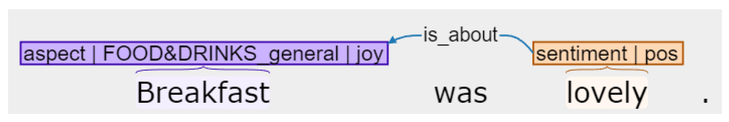
As data for the experiments, we used FMCG (Fast Moving Consumer Goods) reviews which were collected and manually labelled in the framework of the multilingual SentEMO project (http://sentemo.org, accessed on 14 January 2023). The dataset consists of product reviews, i.e., almost 900 reviews in the training set and nearly 400 in the test set. Each review comprises one or more sentences, while each may contain several or no “aspect terms”, which are words or collocations which have been assigned three labels, namely an aspect class, sentiment class and emotion class (we will refer to them as “gold labels”). This annotation is exemplified in Figure 1 for the term “breakfast”, which is assigned the aspect class “Food&Drinks_general”, and for which a positive sentiment is expressed, as well as the emotion, “joy”.
Each of these annotations results in a set of classification labels, which we will consider as three separate tasks in the classification experiments:
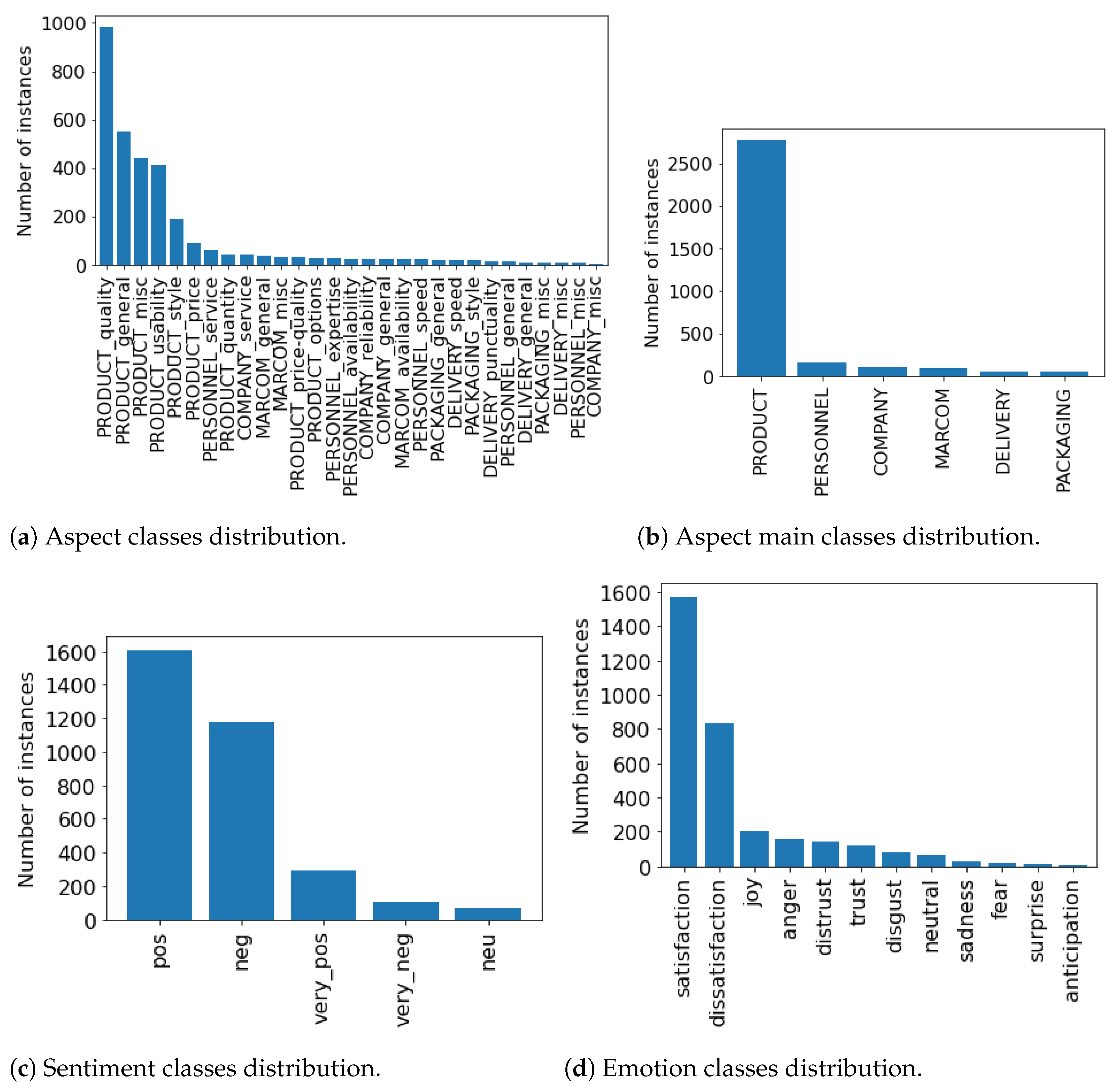
- For the aspect category classification, we consider six main categories (“product”, “personnel”, “company”, “marcom”, “delivery”, and “packaging”; Figure 2b), and each category is further divided into subcategories (“product_quality”, “product_general”, etc.; Figure 2a), which results in a total of 29 classes.
- For sentiment classification, we distinguish five ordinal labels: “very positive”, “positive”, “neutral”, “negative”, and “very negative” (Figure 2c).
- For emotions, there are 12 associated labels: “anger”, “neutral”, “disgust”, “surprise”, “trust”, “distrust”, “dissatisfaction”, “fear”, “joy”, “satisfaction”, “anticipation”, and “sadness” (Figure 2d).
For each of the three tasks, the class distribution is skewed, as is also clearly visualised in Figure 2. While the large majority of instances fall within the “product” category, the sentiment and emotion annotations are also primarily situated in 2 out of the available 5 (sentiment) or 12 (emotion) classes.
4. Methodology
In this section, we provide the theoretical background supporting our approach. In Section 4.1, we briefly describe how the data were presented to us and which data preprocessing steps we considered. Further, in Section 4.2, we list the text embedding methods that we use to prepare the text for the classifiers that we describe in Section 4.3. Finally, in Section 4.4, we discuss the evaluation metrics used to measure the quality of the obtained predictions.
4.1. Data Preprocessing
For our experiments, we selected each term as a separate data instance with all corresponding information, such as the ordinal number of the review, the original full sentence, and the individual classification task labels. We decided not to use any additional text preprocessing to the text before its usage in the embedding methods in order not to dismiss any potentially helpful information.
On the other hand, we tried to provide different text spans to the embedding method (described in Section 4.2) and more specifically considered four options:
- The target term (it can be one word or a collocation).
- The sentence that contains our target term (this could be repeated for different instances because one sentence can contain several terms).
- The combination of the previous two vectors, or the so-called “merged” vector of term and sentence vectors (in this way, this embedding vector’s length will be double the previous one).
- A window of terms, which means that we take into account the words around the target term. We considered windows with sizes of three and five; if a sentence has fewer words before or after the target term, we take as much as it has. We also tried two approaches to apply the embedding: for the first approach, we compute the vector embedding for each word in the window separately and then calculate its mean, while for the second approach, we take the embedding of the whole piece of text.
4.2. Text Embeddings
To be able to use text in the fuzzy-rough classification models, we first need to transform it into an N-dimensional vector form. Methods that perform such a task are called “embedding models”, and they follow the same principle: similar pieces of text should be represented in the N-dimensional space by close vectors. Since the original Word2Vec models, first introduced in [30,31], embedding methods have come a long way, and the state-of-the-art in the NLP field now focuses on transformer encoders. The original BERT model was described in [32] with the idea of pre-training deep bidirectional representations using unlabelled text. The original BERT tasks were language modelling and next-sentence prediction. However, to fine-tune this model, there is no need to modify its architecture, and it can be achieved by adding extra output layers. In our work, we considered several BERT-based models, including the BERT and ALBERT models by TextAttack (https://huggingface.co/textattack/bert-base-uncased-yelp-polarity, accessed on 14 January 2023) fine-tuned using the TextAttack package [33] and the YELP polarity dataset [34] for the sequence classification task.
However, the best results for our experiments were obtained with the DistilBERT Yelp Review Sentiment model (https://huggingface.co/spentaur/yelp, accessed on 14 January 2023) that was fine-tuned on one million reviews from the YELP dataset [34] for the sentiment analysis task. The DistilBERT architecture is a lighter and faster version of BERT that takes less time to fine-tune. As this particular DistilBERT model outperformed both BERT and ALBERT models, in Section 5, we provide the results only for this best embedding method.
All mentioned BERT-based models were fine-tuned on the YELP dataset that contains user reviews from yelp.com, accessed on 14 January 2023. We chose such models due to the similar nature of the data used for their fine-tuning and ours. Although these models were used as classification/regression models for the sequence classification and sentiment analysis tasks, we will use them as embedding models by extracting the encoded vector representations of text.
4.3. Classification Methods
As a classification model, we considered two fuzzy rough set-based methods:
- Fuzzy-Rough Nearest Neighbour (FRNN) is an instance-based classification model proposed by [35], which classifies instances using their lower and upper approximations from fuzzy rough set theory. Particularly, we used the FRNN extension with ordered weighted average (OWA) operators [36] called FRNN-OWA, as described in [37]. To represent the similarity among our instances, we used cosine similarity.
- Fuzzy Rough OVO COmbination (FROVOCO) is also an instance-based algorithm, introduced in [26]. FROVOCO is developed for multi-class classification and especially for imbalanced tasks, which could be suitable given the imbalance present in our data. It decomposes several classes into separate one-vs.-one and one-vs.-rest tasks. For each pair, FROVOCO considers the constructed classes’ imbalance ratio to use specific weights. For this method, we used the recommended Manhattan distance metric.
For both methods, we used additive weights—a vector with a length corresponding to the parameter k (the number of neighbours) with linearly decreasing weights. We took both implementations of FRNN-OWA and FROVOCO from [38] provided at the corresponding GitHub page (https://github.com/oulenz/fuzzy-rough-learn, accessed on 14 January 2023).
4.4. Evaluation Metrics
We used three metrics to measure the performance of considered approaches, viz. F1-score, accuracy, and Cost Corrected Accuracy (CCA).
The F1-score (1) corresponds to the harmonic mean of two other metrics: Precision and Recall:
where the Precision metric represents the ratio of correctly predicted labels out of all predicted labels, and Recall corresponds to the ratio of correctly predicted instances out of all instances with ground-truth labels. F1-score is a suitable metric for an imbalanced dataset. For our experiments, we calculated the weighted F1-score, which is first computed for each label separately, and then the output is their average (weighted by support scores) (https://scikit-learn.org/stable/modules/generated/sklearn.metrics.f1_score.html, accessed on 14 January 2023).
Another evaluation metric that we use in our experiments is accuracy. It corresponds to the number of correctly predicted instances out of all instances in the dataset. It is not the most suitable metric for imbalanced datasets. Still, in our case, it reflects how many data instances are actually left after all the steps of the considered pipelines with data filtration are passed.
As an alternative to accuracy, we also calculated the CCA metric, introduced by [39]. This metric applies to ordinal classification tasks only and is similar to accuracy. However, CCA takes into account the cost of prediction. In other words, for ordinal classes, the prediction of a class close to the actual one (i.e., to the gold label) should have a lower cost than a prediction of a class which is further removed. As a simple example, we can consider a polarity classification task with ordered labels “positive”, “neutral”, and “negative”. Then, we can set up costs in a way that, for instance, with a gold label “positive”, a correctly predicted label will have a cost of 0; a prediction of “neutral” has an associated cost of 1/2, while predicting the “negative” label will correspond to the full cost of 1. Based on this information, we can construct a cost matrix, which is symmetrical with classes on the rows and columns, 0 on the diagonal and the cost of each “prediction mistake” on other positions. Then, having the confusion matrix Cf and a cost matrix Ct, we can calculate CCA with Formula (2):
In this way, higher CCA scores will correspond to better methods in the same way as accuracy, which can be observed as its special case with the cost of each prediction mistake equal to 1. In our experiments, we can apply CCA only for the sentiment and emotion tasks since, for aspect classification, we do not have ordered classes. For both those tasks, we provided the cost matrices in Appendix A Table A1 and Table A2, respectively.
4.5. Pipelines
While others have already investigated tackling some of the ABSA subtasks jointly [40,41,42], the predominant methodology in ABSA is still a pipeline approach in which the first aspect categorisation is performed, and after which the sentiment and emotion labels are predicted for the predicted aspect categories. These pipeline approaches are known to be sensitive to error propagation, which might be even more the case for the imbalanced datasets we are working with. In our experiments, we want to investigate different pipelines and their error and more specifically study how fuzzy rough-set-based methods such as FRNN-OWA, but also FROVOCO, which is specifically designed to handle imbalanced datasets, behave in such a pipeline setup.
Before describing the actual pipeline for the ABSA task, we should mention some preparatory steps that we performed. First of all, we aimed to detect the best classification model setup for each task separately (i.e., aspect, sentiment, and emotion classification) based on gold labels and cross-validation (CV) evaluation. For this purpose, for each task, we computed predictions using various classification models and different text spans for the text embeddings and tuned each model’s parameters. Through this, using CV, we were able to define the best approach for each classification task.
These best models were then applied one by one, forming the “pipeline” for the ABSA task. First, the best “aspect model” was applied to predict aspect classes for all test set instances. Then, the best “sentiment model” was evaluated on the instances with correctly predicted aspect labels, after which the “emotion model” was applied to the instances which were correctly predicted in the previous step. Contrary to a normal test scenario, in which we evidently do not have access to gold standard annotations, this approach of only taking into account the correctly predicted instances for the next step primarily enabled us to assess the error propagation throughout the classification pipeline.
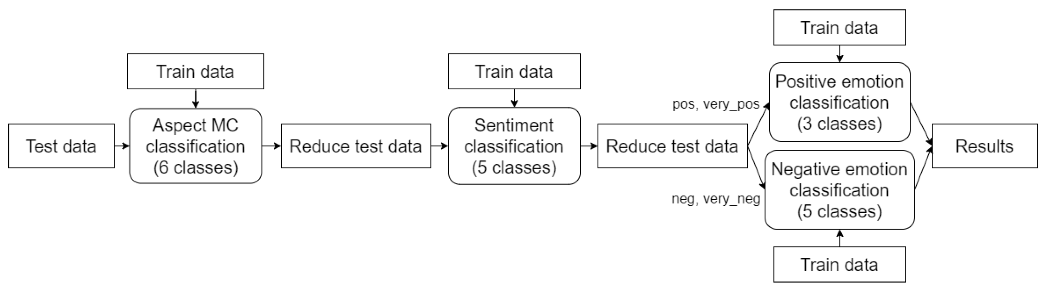
We improved this baseline approach with two modifications. First of all, as was showcased in Figure 2a, the class distribution of the aspect categories is highly imbalanced. Since there was simply too little training data for the large majority of aspect categories, we generalised the 29 aspect classes into 6 main categories as discussed in Section 3. A second modification we considered is splitting the emotion models into positive and negative ones. We thus divided the gold emotion labels into two groups; some of them we joined into one emotion class due to the similar nature of the emotions and the small size of their classes:
- Three positive emotions: joy combined with anticipation and “positive” surprise (instances that have emotion gold label “surprise” and sentiment gold labels “positive” or “very positive”); satisfaction; and trust.
- Five negative emotions: anger; disgust; dissatisfaction; distrust merged with fear; and sadness combined with “negative” surprise (instances that have emotion gold label “surprise” and sentiment gold labels “negative” or “very negative”).
For the model tuning on the gold standard, we divided the training instances into two groups based on their gold emotion labels (positive and negative). However, for the pipeline approach, the approach had to be different. Since we base our emotion prediction step on sentiment classification results, we use the predicted sentiment labels to divide instances into three groups. We combine all instances with “positive” and “very positive” sentiment labels and apply a positive emotion model setup. A similar procedure is conducted for the “negative” and “very negative” sentiment labels. The remaining instances have a “neutral” sentiment label and are automatically assigned the “neutral” emotion. We call the described pipeline “System 1”, which is illustrated in Figure 3. To illustrate how System 1 works, we can take a look at the test example: “The staff was very friendly, but the breakfast could have been better”. “Staff” has the gold labels “personnel” as aspect category, “positive” as sentiment and “joy” as emotion; the corresponding labels for “breakfast” are “food&drinks”, “negative” and “dissatisfaction”. If System 1, for example, erroneously predicts “breakfast” as “very negative”, this instance will not be taken into account anymore for emotion prediction.
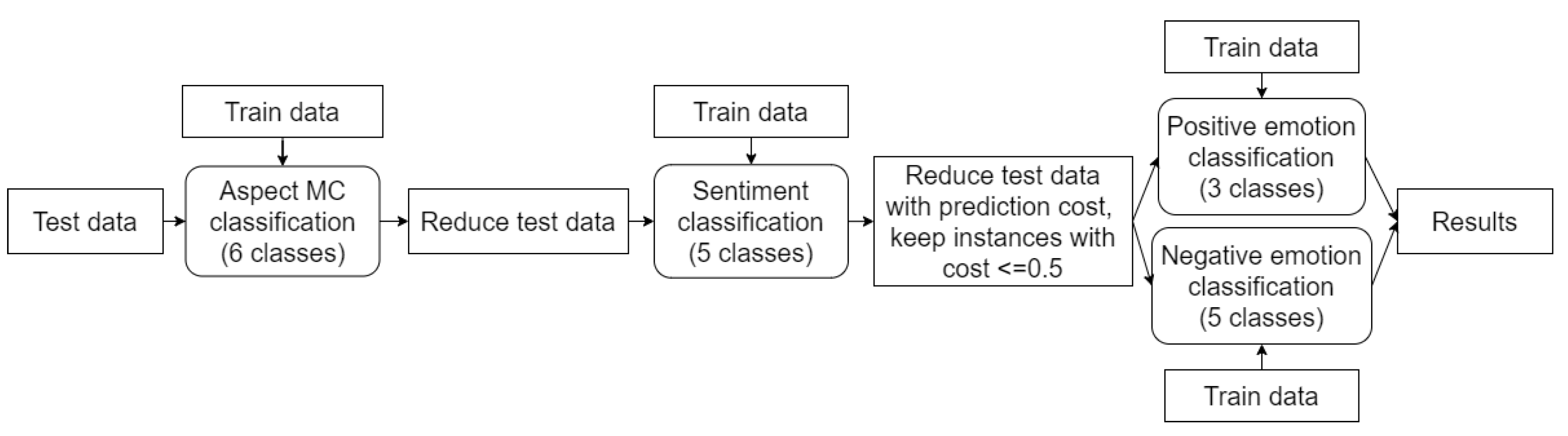
We also considered a more relaxed pipeline. For “System 2” (Figure 4), we perform data reduction with the cost matrices described in Section 4.4. Since the first step (aspect classification) is not an ordinal task, and we do not have a cost matrix for it, this approach is only relevant for the latter two tasks. While in System 1, we only kept instances for further processing when they had a cost of “0”; we now also keep instances with a cost “0.5”. This modification allows us to bring more instances to the emotion detection step. However, the scores for aspect and sentiment detection evidently will remain the same.
When we come back to our test example and use System 2 on it, we predictably will receive the same aspect and sentiment labels as System 1. However, the cost of our sentiment classification mistake will be 0.5, which is acceptable. The subsequent emotion detection step leads to the predicted emotional class, “dissatisfaction”, which is actually correct.
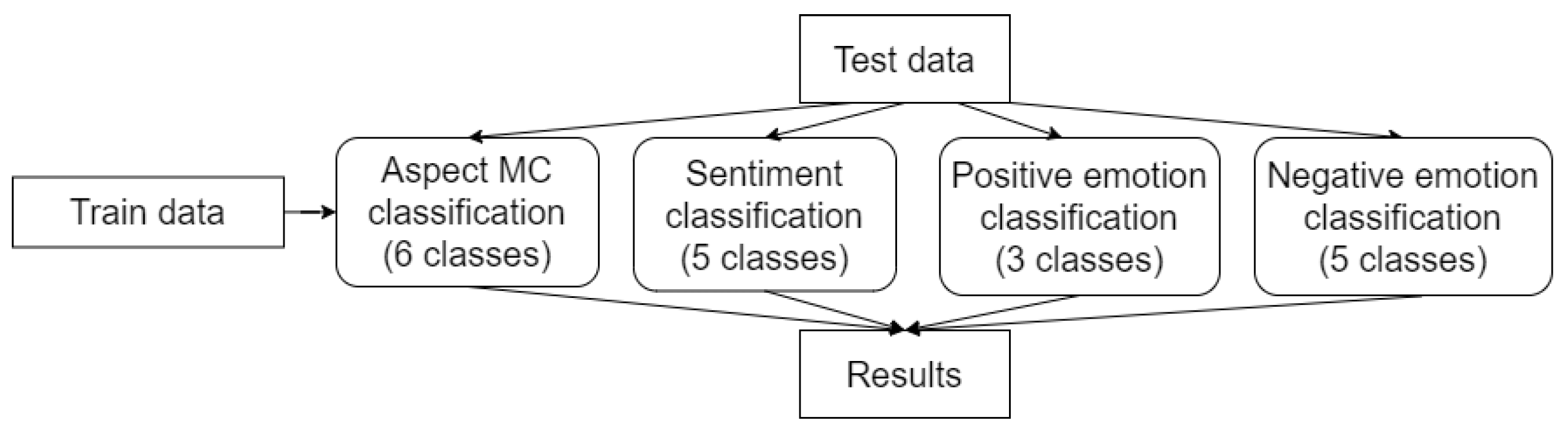
Finally, in “System 3”, we make our three classification steps independent (Figure 5) of each other, giving us an idea of the performance of each of the classifiers on the complete test data. In fact, this third system can be observed as the upperbound for the previous two pipeline systems, in which a test instance is only counted correct if all three classification predictions are correct.
5. Results
In this section, we provide the results obtained from our experiments. First, in Section 5.1, we describe the best model setup tuned for each classification task based on gold labels. Then, in Section 5.2, we provide results for our three systems based on the models from Section 5.1.
5.1. Detecting the Best Setup for Each Classification Task
To achieve the highest possible scores in the pipeline, we should be sure that we receive the best results on each classification step. With this idea, we tuned the best model for each task of the three classification steps: aspect category classification, sentiment and emotion classification. For each of them, we compared two classification models (FRNN-OWA and FROVOCO), four text spans for the text embedding technique (term, sentence, window of words and combined vectors of term and sentence), and finally tuned the model parameter k (the number of neighbours), trying odd values from 1 to 29. We used the F1-score for the fivefold cross-validation to evaluate the results based on gold labels. The obtained scores are provided in Table 1. All provided results are presented for the DistilBERT text embedding.
In Table 1, “Aspect Main Categories” corresponds to the aspect classification task with six main category classes, while “Positive Emotions” and “Negative Emotions” stand for the positive and negative emotion models explained in Section 4.5. When we consider the text spans, “merged” means the merged vector of term and sentence, and “w5 whole” stands for the usage of an embedding vector generated for the text span obtained with a window size of five around the target term.
From Table 1, we can observe that we obtained the highest F1-score for the aspect classification task and the lowest for the negative emotion prediction. Regarding the classification model of choice, FRNN-OWA and FROVOCO are both selected as best classifier for two of the four classification tasks. As for the text spans, we can say that the option of the “merged” vector was always better than the terms and the sentence vectors. A window of terms approach only outperformed the merged vector setup once, namely for the sentiment classification task. A window with size five and an embedding taking into account the whole text span was always the strongest approach compared to the other windows’ setups.
5.2. Systems
Once we obtained the best setup for each classification task, we combined them in the three systems described in Section 4.5. For each system, we measured the F1-score, accuracy, and CCA for each of the three classification tasks: aspect, sentiment and emotion classification. The results for all three systems are provided in Table 2.
As we can observe from Table 2, the separate systems from System 3 yield performances of 86.3% for aspect categorisation (accuracy), 84.6% for sentiment analysis (CCA) and 81.4% for emotion detection (CCA). When we consider the first two pipeline systems, the results evidently drop because an error in the previous step negatively impacts the following step. Furthermore, the cost-driven filtering of the instances seems to pay off.
6. Error Analysis
We manually explored some correctly and incorrectly predicted test instances for each classification task to assess the performance of our FRNN approach. In doing so, we went back into our solution to find neighbouring training instances to the considered test instance. For each classification task’s best setup, we calculated the top k nearest neighbours to the target test instance and examined those neighbours in order to find patterns in these neighbouring instances.
First, we considered a test sample that obtained the wrong sentiment prediction for all systems:
Example 1.
In fact, I will likely buy a second.
From here on, for each example we will label a term with an underline. For Example 1, its gold aspect main label “product” was correctly predicted by all three systems. However, the gold sentiment label “positive” was misclassified by all systems as “negative”. It leads to no emotion prediction for Systems 1 and 2 when System 3 predicted “dissatisfaction”, which is the opposite to gold “trust”, but was logical for the predicted negative sentiment.
Taking a look at the training neighbours for the sentiment task (Table 3), we can observe that the majority of them represent negative feedback. Those examples demonstrate that they all have a common topic—the impression of the product that influences the user’s decision to repurchase it or to recommend this product to others. We can suggest that due to the high amount of examples where users were dissatisfied with their products, we can have a lot of negative neighbours for our test example, which leads to a wrong prediction. Hence, the same topic can be a substantial similarity feature for our approach.
Second, we take a look at a test sample, where the sentiment was wrong with a low cost:
Example 2.
We use these in our bathrooms and kitchen and believe they work very well.
Again, the aspect class “product” was predicted correctly by all systems, while the gold sentiment label “very positive” was predicted as “positive”. Because of that, System 1 cannot predict emotion; however, System 2 can because the cost of this mistake is 0.5, and we allowed it. Due to this, System 2 predicts the “satisfaction” emotion, which corresponds to the prediction of System 3 and the gold label.
If we take a look at some of the neighbouring training instances (Table 4), we can observe that all neighbours are either “positive” or “very positive”, so it is easy to confuse. Meanwhile, we can also notice an interesting pattern—the common thing among those neighbours is not a topic but rather positive words, such as “work well” (the same collocation as in the test example), “very professional”, “very happy”, and others. We can conclude that words with high emotional colouring could be a trigger for our similarity algorithm.
Third, we considered a test example, where all systems guessed the sentiment correctly:
Example 3.
It has NO SENSOR for odor detection; therefore, it will not automatically change the fan setting if unwelcomed odors were to invade the space.
While the gold aspect main label “product” and gold sentiment label “negative” were correctly predicted by all three systems, for the emotion label, all systems made a mistake, as instead of the gold emotion label “anger”, for each system “dissatisfaction” was predicted. To investigate that, we can take a look at the neighbouring training instances to the corresponding test one in Table 5.
While the majority of neighbours have the label “dissatisfaction” (or “anger”), actually, the closest sentence by meaning is the first sentence that is labelled with “satisfaction”. However, the content of the first neighbour seems rather disappointing and negatively toned. In this way, we can confirm our preliminary conclusions that the common topic seems to be a strong feature that marks the neighbours. Moreover, we can notice that some training instances can have confusing or even unsuitable labels. We cannot dismiss the fact that similar emotions, such as anger and dissatisfaction, could be easily confused due to the subjectivity of emotions, which again shows the usefulness of the CCA metric.
Finally, we take a look at some test examples that were predicted with a wrong aspect label (gold aspect classes are provided between brackets):
Example 4.
- 1.
- This shampoo did not come spilled, packaged to perfection (“packaging”).
- 2.
- There are good sales people (“personnel”).
- 3.
- Dishonest company and seller (“company”).
All those texts were predicted as “product”, which can be expected due to the huge unbalance of the data. For this reason, we have no predictions for the sentiment and emotion labels from Systems 1 and 2; meanwhile, System 3 predicted them correctly for each sample (“positive” and “satisfaction” for Example 4(1) and Example 4(2), and “negative” and “distrust” for Example 4(3)). What is curious about those examples is that they all are quite short and still have some emotionally strong words that can appear in their neighbours: “perfect” for the first, “good” for the second, and “dishonest” (“horrible”, “awful”) for the third.
To conclude, we can say that human emotions are very subjective concepts that can lead to contradictory instance labelling and unexpected patterns chosen by the system. By a manual analysis of the output and the nearest neighbours of both the OWA-FRNN and FROVOCO systems, we can inspect which instances lead to a given classification decision, gaining more insights in the underlying data. This not only enables us to find some explanations for classification decisions, but can also aid us in pinpointing errors, shortcomings or even biases in the underlying data as a basis for improving our future work.
7. Conclusions and Future Work
In this work, we have considered two fuzzy rough set-based machine learning techniques for the task of Aspect-Based Sentiment Analysis. It gives novelty to our solution since interpretability was not investigated much for considered emotion-detection tasks before, as well as the usage of DL-based and BERT-based embedding techniques with the instance-based fuzzy-rough-based approaches. We used them to approach the ABSA task, which in our setup consists of three subtasks: aspect, sentiment and emotion classification, and which we tackle using a pipeline approach. For each of these subtasks, we implemented the fuzzy rough set-based methods FRNN-OWA and FROVOCO using transformers-based text embeddings and showed high results on the test data (up to 0.86 accuracy score for aspect categorisation, 0.84 CCA for sentiment analysis and 0.81 CCA for emotion detection). In addition, our solution is interpretable in a local, self-explaining, example-driven way. Through error analysis, we demonstrated that our approaches could identify helpful patterns from the results that can update future models.
Since [2] used the Dutch version of the dataset, while we were working with an English one, we could not thoroughly compare our results. However, we used the same evaluation metrics, such as F1-score and CCA, to approximate the quality of our performance. In general, we can observe that our results were in line (classification of sentiment and emotions) or even slightly higher (classification of main aspects).
In future work, we plan to address the problem of unbalanced data and explore a more systematic method to analyse the solution’s interpretability. Moreover, we can try to apply the extracted patterns from the previous models to improve the next ones.
Author Contributions
O.K., Conceptualisation, Methodology, Software, Validation, Formal analysis, Investigation Data curation, Writing original draft and Visualisation. C.C., Supervision, Resources and Writing—review and editing. V.H., Supervision, Resources, and Writing—review and editing. All authors have read and agreed to the published version of the manuscript.
Funding
Olha Kaminska and Chris Cornelis would like to thank the Odysseus project from Flanders Research Foundation (FWO), Grant No. G0H9118N, for funding their research.
Institutional Review Board Statement
Not applicable.
Informed Consent Statement
Not applicable.
Data Availability Statement
Acknowledgments
We would like to thank Ellen De Geyndt for providing the data and consultation regarding the pipeline developing.
Conflicts of Interest
The authors declare no conflict of interest.
Appendix A. Cost Matrices

Table A1.
Sentiment Cost Matrix.
| Negative | Neutral | Positive | Very_Negative | Very_Positive | |
|---|---|---|---|---|---|
| Negative | 0 | 0.5 | 1 | 0.5 | 1 |
| Neutral | 0.5 | 0 | 0.5 | 0.5 | 0.5 |
| Positive | 1 | 0.5 | 0 | 1 | 0.5 |
| very_negative | 0.5 | 0.5 | 1 | 0 | 1 |
| very_positive | 1 | 0.5 | 0.5 | 1 | 0 |
Table A2.
Emotion Cost Matrix.
| Anger | Anticipation | Disgust | Dissatisfaction | Distrust | Fear | Joy | Neutral | Sadness | Satisfaction | Surprise | Trust | |
|---|---|---|---|---|---|---|---|---|---|---|---|---|
| Anger | 0 | 1 | 0.25 | 0.5 | 0.25 | 0.25 | 1 | 0.75 | 0.25 | 1 | 0.25 | 1 |
| Anticipation | 1 | 0 | 1 | 1 | 1 | 1 | 0.25 | 0.75 | 1 | 0.5 | 0.25 | 0.25 |
| Disgust | 0.25 | 1 | 0.25 | 0.5 | 0 | 0.25 | 1 | 0.75 | 0.25 | 1 | 0.25 | 1 |
| Dissatisfaction | 0.5 | 1 | 0.5 | 0 | 0.5 | 0.5 | 1 | 0.5 | 0.5 | 1 | 0.25 | 1 |
| Distrust | 0.25 | 1 | 0 | 0.5 | 0.25 | 0.25 | 1 | 0.75 | 0.25 | 1 | 0.25 | 1 |
| Fear | 0.25 | 1 | 0.25 | 0.5 | 0.25 | 0 | 1 | 0.75 | 0.25 | 1 | 0.25 | 1 |
| Joy | 1 | 0.25 | 1 | 1 | 1 | 1 | 0 | 0.75 | 1 | 0.5 | 0.25 | 0.25 |
| Neutral | 0.75 | 0.75 | 0.75 | 0.5 | 0.75 | 0.75 | 0.75 | 0 | 0.75 | 0.5 | 0.75 | 0.75 |
| Sadness | 0.25 | 1 | 0.25 | 0.5 | 0.25 | 0.25 | 1 | 0.75 | 0 | 1 | 0.25 | 1 |
| Satisfaction | 1 | 0.5 | 1 | 1 | 1 | 1 | 0.5 | 0.5 | 1 | 0 | 0.25 | 0.5 |
| Surprise | 1 | 0.25 | 1 | 1 | 1 | 1 | 0.25 | 0.75 | 1 | 0.5 | 0.25 | 0 |
| Trust | 0.25 | 0.25 | 0.25 | 0.5 | 0.25 | 0.25 | 0.25 | 0.75 | 0.25 | 0.5 | 0 | 0.25 |
References
- Liu, B. Sentiment analysis and opinion mining. Synth. Lect. Hum. Lang. Technol. 2012, 5, 1–167. [Google Scholar]
- De Geyndt, E.; De Clercq, O.; Van Hee, C.; Lefever, E.; Singh, P.; Parent, O.; Hoste, V. SentEMO: A Multilingual Adaptive Platform for Aspect-based Sentiment and Emotion Analysis. In Proceedings of the 12th Workshop on Computational Approaches to Subjectivity, Sentiment & Social Media Analysis, Collocated with Association for Computational Linguistics, Dublin, Ireland, 23–25 May 2022; pp. 51–61. [Google Scholar]
- Kaminska, O.; Cornelis, C.; Hoste, V. Fuzzy-Rough Nearest Neighbour Approaches for Emotion Detection in Tweets. In Proceedings of the Rough Sets, Bratislava, Slovakia, 19–24 September 2021; Springer International Publishing: Berlin/Heidelberg, Germany, 2021. [Google Scholar]
- Kaminska, O.; Cornelis, C.; Hoste, V. LT3 at SemEval-2022 Task 6: Fuzzy-Rough Nearest Neighbor Classification for Sarcasm Detection. In Proceedings of the 16th International Workshop on Semantic Evaluation (SemEval-2022), Online, 14–15 July 2022; Association for Computational Linguistics: Seattle, WA, USA, 2022; pp. 987–992. [Google Scholar] [CrossRef]
- Kaminska, O.; Cornelis, C.; Hoste, V. Fuzzy rough nearest neighbour methods for detecting emotions, hate speech and irony. Inf. Sci. 2023, 625, 521–535. [Google Scholar] [CrossRef]
- Hu, M.; Liu, B. Mining and summarizing customer reviews. In Proceedings of the Tenth ACM SIGKDD International Conference on Knowledge Discovery and Data Mining, Seattle, WA, USA, 22–25 August 2004; pp. 168–177. [Google Scholar]
- Li, X.; Bing, L.; Zhang, W.; Lam, W. Exploiting BERT for End-to-End Aspect-based Sentiment Analysis. In Proceedings of the 5th Workshop on Noisy User-Generated Text (W-NUT 2019), Hong Kong, China, 4 November 2019; Association for Computational Linguistics: Hong Kong, China, 2019. [Google Scholar]
- Karimi, A.; Rossi, L.; Prati, A. Adversarial training for aspect-based sentiment analysis with bert. In Proceedings of the 2020 25th International Conference on Pattern Recognition (ICPR), Milan, Italy, 10–15 January 2021; pp. 8797–8803. [Google Scholar]
- Zhao, A.; Yu, Y. Knowledge-enabled BERT for aspect-based sentiment analysis. Knowl.-Based Syst. 2021, 227, 107220. [Google Scholar] [CrossRef]
- Yang, L.; Na, J.C.; Yu, J. Cross-modal multitask transformer for end-to-end multimodal aspect-based sentiment analysis. Inf. Process. Manag. 2022, 59, 103038. [Google Scholar] [CrossRef]
- Pontiki, M.; Galanis, D.; Pavlopoulos, J.; Papageorgiou, H.; Androutsopoulos, I.; Manandhar, S. SemEval-2014 Task 4: Aspect Based Sentiment Analysis. In Proceedings of the 8th International Workshop on Semantic Evaluation (SemEval 2014), Dublin, Ireland, 23–24 August 2014; Association for Computational Linguistics: Dublin, Ireland, 2014; pp. 27–35. [Google Scholar] [CrossRef] [Green Version]
- Pontiki, M.; Galanis, D.; Papageorgiou, H.; Manandhar, S.; Androutsopoulos, I. SemEval-2015 Task 12: Aspect Based Sentiment Analysis. In Proceedings of the 9th International Workshop on Semantic Evaluation (SemEval 2015), Denver, CO, USA, 4–5 June 2015; Association for Computational Linguistics: Denver, CO, USA, 2015; pp. 486–495. [Google Scholar] [CrossRef] [Green Version]
- Pontiki, M.; Galanis, D.; Papageorgiou, H.; Androutsopoulos, I.; Manandhar, S.; AL-Smadi, M.; Al-Ayyoub, M.; Zhao, Y.; Qin, B.; De Clercq, O.; et al. SemEval-2016 Task 5: Aspect Based Sentiment Analysis. In Proceedings of the 10th International Workshop on Semantic Evaluation (SemEval-2016), San Diego, CA, USA, 16–17 June 2016; Association for Computational Linguistics: San Diego, CA, USA, 2016; pp. 19–30. [Google Scholar] [CrossRef] [Green Version]
- Danilevsky, M.; Qian, K.; Aharonov, R.; Katsis, Y.; Kawas, B.; Sen, P. A Survey of the State of Explainable AI for Natural Language Processing. In Proceedings of the 1st Conference of the Asia-Pacific Chapter of the Association for Computational Linguistics and the 10th International Joint Conference on Natural Language Processing, Suzhou, China, 4–7 December 2020; Association for Computational Linguistics: Suzhou, China, 2020; pp. 447–459. [Google Scholar]
- Wu, Z.; Chen, Y.; Kao, B.; Liu, Q. Perturbed masking: Parameter-free probing for analyzing and interpreting BERT. arXiv 2020, arXiv:2004.14786. [Google Scholar]
- Ribeiro, M.T.; Singh, S.; Guestrin, C. “Why should I trust you?” Explaining the predictions of any classifier. In Proceedings of the 22nd ACM SIGKDD International Conference on Knowledge Discovery and Data Mining, San Francisco, CA, USA, 13–17 August 2016; pp. 1135–1144. [Google Scholar]
- Strumbelj, E.; Kononenko, I. An efficient explanation of individual classifications using game theory. J. Mach. Learn. Res. 2010, 11, 1–18. [Google Scholar]
- Yang, Z.; Yang, D.; Dyer, C.; He, X.; Smola, A.; Hovy, E. Hierarchical attention networks for document classification. In Proceedings of the 2016 Conference of the North American Chapter of the Association for Computational Linguistics: Human Language Technologies, San Diego, CA, USA, 12–17 June 2016; Association for Computational Linguistics: San Diego, CA, USA, 2016; pp. 1480–1489. [Google Scholar]
- Chen, H.; Ji, Y. Learning variational word masks to improve the interpretability of neural text classifiers. arXiv 2020, arXiv:2010.00667. [Google Scholar]
- Bahdanau, D.; Cho, K.H.; Bengio, Y. Neural machine translation by jointly learning to align and translate. In Proceedings of the 3rd International Conference on Learning Representations, ICLR 2015, San Diego, CA, USA, 7–9 May 2015. [Google Scholar]
- Li, J.; Chen, X.; Hovy, E.; Jurafsky, D. Visualizing and Understanding Neural Models in NLP. In Proceedings of the NAACL-HLT, San Diego, CA, USA, 12–17 June 2016; pp. 681–691. [Google Scholar]
- Croce, D.; Rossini, D.; Basili, R. Auditing deep learning processes through kernel-based explanatory models. In Proceedings of the 2019 Conference on Empirical Methods in Natural Language Processing and the 9th International Joint Conference on Natural Language Processing (EMNLP-IJCNLP), Hong Kong, China, 3–7 November 2019; Association for Computational Linguistics: Hong Kong, China, 2019; pp. 4037–4046. [Google Scholar]
- Jiang, Y.; Joshi, N.; Chen, Y.-C.; Bansal, M. Explore, Propose, and Assemble: An Interpretable Model for Multi-Hop Reading Comprehension. In Proceedings of the 57th Annual Meeting of the Association for Computational Linguistics, Florence, Italy, 28 July–2 August 2019; pp. 2714–2725. [Google Scholar]
- Vluymans, S.; D’eer, L.; Saeys, Y.; Cornelis, C. Applications of fuzzy rough set theory in machine learning: A survey. Fundam. Inform. 2015, 142, 53–86. [Google Scholar] [CrossRef] [Green Version]
- Zhao, S.; Tsang, E.; Chen, D.; Wang, X. Building a Rule-Based Classifier—A Fuzzy-Rough Set Approach. IEEE Trans. Knowl. Data Eng. 2010, 22, 624–638. [Google Scholar] [CrossRef]
- Vluymans, S.; Fernández, A.; Saeys, Y.; Cornelis, C.; Herrera, F. Dynamic affinity-based classification of multi-class imbalanced data with one-versus-one decomposition: A fuzzy rough set approach. Knowl. Inf. Syst. 2018, 56, 55–84. [Google Scholar] [CrossRef]
- Zhao, J.Y.; Zhang, Z.L. Fuzzy rough neural network and its application to feature selection. In Proceedings of the 4th International Workshop on Advanced Computational Intelligence, Wuhan, China, 19–21 October 2011; pp. 684–687. [Google Scholar]
- Kaminska, O.; Cornelis, C.; Hoste, V. Nearest neighbour approaches for Emotion Detection in Tweets. In Proceedings of the 11th Workshop on Computational Approaches to Subjectivity, Sentiment and Social Media Analysis, Online, 19–23 April 2021; pp. 203–212. [Google Scholar]
- Mohammad, S.M.; Bravo-Marquez, F.; Salameh, M.; Kiritchenko, S. SemEval-2018 Task 1: Affect in Tweets. In Proceedings of the International Workshop on Semantic Evaluation (SemEval-2018), New Orleans, LA, USA, 5–6 June 2018. [Google Scholar]
- Mikolov, T.; Chen, K.; Corrado, G.; Dean, J. Efficient Estimation of Word Representations in Vector Space. arXiv 2013, arXiv:1301.3781. [Google Scholar]
- Mikolov, T.; Sutskever, I.; Chen, K.; Corrado, G.; Dean, J. Distributed Representations of Words and Phrases and Their Compositionality. In Proceedings of the 26th International Conference on Neural Information Processing Systems—Volume 2, Lake Tahoe, NV, USA, 5–10 December 2013; NIPS’13. pp. 3111–3119. [Google Scholar]
- Devlin, J.; Chang, M.W.; Lee, K.; Toutanova, K. BERT: Pre-training of Deep Bidirectional Transformers for Language Understanding. In Proceedings of the 2019 Conference of the North American Chapter of the Association for Computational Linguistics: Human Language Technologies, Volume 1 (Long and Short Papers), Minneapolis, MN, USA, 2–7 June 2019; pp. 4171–4186. [Google Scholar]
- Morris, J.; Lifland, E.; Yoo, J.Y.; Grigsby, J.; Jin, D.; Qi, Y. TextAttack: A Framework for Adversarial Attacks, Data Augmentation, and Adversarial Training in NLP. In Proceedings of the 2020 Conference on Empirical Methods in Natural Language Processing: System Demonstrations, Online, 16–20 November 2020; pp. 119–126. [Google Scholar]
- Zhang, X.; Zhao, J.; LeCun, Y. Character-Level Convolutional Networks for Text Classification. arXiv 2015, arXiv:1509.01626. [Google Scholar]
- Jensen, R.; Cornelis, C. Fuzzy-rough nearest neighbour classification and prediction. Theor. Comput. Sci. 2011, 412, 5871–5884. [Google Scholar] [CrossRef] [Green Version]
- Vluymans, S.; Mac Parthaláin, N.; Cornelis, C.; Saeys, Y. Weight selection strategies for ordered weighted average based fuzzy rough sets. Inf. Sci. 2019, 501, 155–171. [Google Scholar] [CrossRef]
- Lenz, O.U.; Peralta, D.; Cornelis, C. Scalable approximate FRNN-OWA classification. IEEE Trans. Fuzzy Syst. 2019, 28, 929–938. [Google Scholar] [CrossRef] [Green Version]
- Lenz, O.U.; Peralta, D.; Cornelis, C. Fuzzy-rough-learn 0.1: A Python library for machine learning with fuzzy rough sets. In Proceedings of the IJCRS 2020: International Joint Conference on Rough Sets, Havana, Cuba, 29 June–3 July 2020; Volume 12179, pp. 491–499. [Google Scholar]
- De Bruyne, L.; De Clercq, O. Prospects for Dutch Emotion Detection: Insights from the New EmotioNL Dataset. Comput. Linguist. Neth. J. 2022, 11, 231–255. [Google Scholar]
- Chen, G.; Tian, Y.; Song, Y. Joint Aspect Extraction and Sentiment Analysis with Directional Graph Convolutional Networks. In Proceedings of the 28th International Conference on Computational Linguistics, Online, 8–13 December 2020; International Committee on Computational Linguistics: Barcelona, Spain, 2020; pp. 272–279. [Google Scholar] [CrossRef]
- Mao, Y.; Shen, Y.; Yu, C.; Cai, L. A joint training dual-mrc framework for aspect based sentiment analysis. AAAI Conf. Artif. Intell. 2021, 35, 13543–13551. [Google Scholar] [CrossRef]
- Wan, H.; Yang, Y.; Du, J.; Liu, Y.; Qi, K.; Pan, J.Z. Target-aspect-sentiment joint detection for aspect-based sentiment analysis. AAAI Conf. Artif. Intell. 2020, 34, 9122–9129. [Google Scholar] [CrossRef]
Figure 1.
Annotation example of the user review with demonstration of aspect, sentiment, and emotion classes of the defined term.
Figure 1.
Annotation example of the user review with demonstration of aspect, sentiment, and emotion classes of the defined term.

Figure 2.
Histograms depicting class distribution for training data for each classification task.

Figure 3.
System 1: pipeline of three classification tasks in sequence with modifications in the form of aspects’ main categories prediction and two emotion models.
Figure 3.
System 1: pipeline of three classification tasks in sequence with modifications in the form of aspects’ main categories prediction and two emotion models.

Figure 4.
System 2: a modification of System 1, where after the sentiment prediction step, data reduction is performed based on misclassification cost.
Figure 4.
System 2: a modification of System 1, where after the sentiment prediction step, data reduction is performed based on misclassification cost.

Figure 5.
System 3: three independent classification tasks on the full test set with no data reduction.
Figure 5.
System 3: three independent classification tasks on the full test set with no data reduction.

Table 1.
Best setup for each individual classification task: aspect, sentiment and emotion prediction.
Table 1.
Best setup for each individual classification task: aspect, sentiment and emotion prediction.
| Task | Model | k | Text Span | F1 CV |
|---|---|---|---|---|
| Aspect Main Categories | FRNN-OWA | 3 | merged | 0.9036 |
| Sentiment | FROVOCO | 9 | w5 whole | 0.7289 |
| Positive Emotions | FRNN-OWA | 9 | merged | 0.8273 |
| Negative Emotions | FROVOCO | 5 | merged | 0.7025 |
Table 2.
Results for all classification tasks for the three systems.
| System | Aspect | Sentiment | Emotion | ||||||
|---|---|---|---|---|---|---|---|---|---|
| F1 | Acc | CCA | F1 | Acc | CCA | F1 | Acc | CCA | |
| 1 | 0.8406 | 0.8627 | - | 0.7147 | 0.6756 | 0.7268 | 0.5647 | 0.4872 | 0.5697 |
| 2 | 0.6155 | 0.5598 | 0.6564 | ||||||
| 3 | 0.7740 | 0.7846 | 0.8458 | 0.6851 | 0.7012 | 0.8142 | |||
Table 3.
Training neighbour instances for Example 1.
| The Full Sentence | Sentiment |
|---|---|
| I plan to return this item and look for a higher quality air purifier. | Negative |
| I will probably not choose Cottonelle Ultra next time around. | Negative |
| I would recommend it for sure, but now I do not have this equipment. | Positive |
| I would HIGHLY suggest you choose another fan, as this one seems to be nothing but one disaster after another. | Very negative |
Table 4.
Training neighbour instances for Example 2.
| The Full Sentence | Sentiment |
|---|---|
| I have worked with them and I think they work well. | Positive |
| They are very responsive, very professional and very present when we need them. | Very positive |
| We are very happy with the product, the machines are reliable and perform. | Very positive |
| They work well and the one we have mounted in our small bathroom helps cut down on the heat in that room, which really builds up as it does not receive air conditioning like the rest of our home. | Positive |
Table 5.
Training neighbour instances for Example 3.
| The Full Sentence | Emotion |
|---|---|
| Unfortunately, upon installing and turning on the air purifier, the output air had a chemical odor smell that is similar to what other reviewers have been describing since 2018. | Satisfaction |
| The error messages with calibrators are annoying though, because they always show up, and it does not say which error it is. | Dissatisfaction |
| Due to the characteristics of immunoassay designs, especially in the free ideas in the measurement of two-step methods, interference and transport disturbances of thyroid hormones are reduced. | Dissatisfaction |
| Your AB and screen choice can be set to activate when you raise your arm, but there is an irritating delay, even when set to the arm raise’s sensitive setting. | Anger |
Disclaimer/Publisher’s Note: The statements, opinions and data contained in all publications are solely those of the individual author(s) and contributor(s) and not of MDPI and/or the editor(s). MDPI and/or the editor(s) disclaim responsibility for any injury to people or property resulting from any ideas, methods, instructions or products referred to in the content. |
© 2023 by the authors. Licensee MDPI, Basel, Switzerland. This article is an open access article distributed under the terms and conditions of the Creative Commons Attribution (CC BY) license (https://creativecommons.org/licenses/by/4.0/).
Share and Cite
MDPI and ACS Style
Kaminska, O.; Cornelis, C.; Hoste, V. Fuzzy Rough Nearest Neighbour Methods for Aspect-Based Sentiment Analysis. Electronics 2023, 12, 1088. https://doi.org/10.3390/electronics12051088
AMA Style
Kaminska O, Cornelis C, Hoste V. Fuzzy Rough Nearest Neighbour Methods for Aspect-Based Sentiment Analysis. Electronics. 2023; 12(5):1088. https://doi.org/10.3390/electronics12051088
Chicago/Turabian StyleKaminska, Olha, Chris Cornelis, and Veronique Hoste. 2023. "Fuzzy Rough Nearest Neighbour Methods for Aspect-Based Sentiment Analysis" Electronics 12, no. 5: 1088. https://doi.org/10.3390/electronics12051088
Note that from the first issue of 2016, this journal uses article numbers instead of page numbers. See further details here.