Permanent Magnet Synchronous Motor Driving Mechanical Transmission Fault Detection and Identification: A Model-Based Diagnosis Approach

Abstract

This paper presents a model-based scheme for permanent magnet synchronous motor (PMSM) driving transmission fault detection and identification (FDI) in a steady-state condition. The proposed framework utilizes a PMSM state-space model and an approximated transmission model to construct the regression models for parameter estimation using the Recursive Least-Square (RLS) algorithm. The FDI are accomplished by the residual current spectrum thresholding method to assess the fault characteristic frequency magnitude and also by parameter clustering. Two types of mechanical transmission with three different fault conditions are tested in the experiments. As a preliminary effort in the condition monitoring of PMSM driving transmission, the study results demonstrate a promising approach by considering both residual current spectrum and parameter cluster, which achieved a satisfactory decision making in detecting and identifying the faulty condition.

1. Introduction

In recent years, PMSMs have been used in many applications such as industrial manufacturing, electric vehicles, and power generation. In these applications, a mechanical transmission is usually implemented to couple the PMSM and the driven load. Due to its role in transmitting the energy from PMSM to the driven load, the transmission is highly exposed to failures. Failures in transmission can lead to severe consequences from production loss to safety issues. Hence, there is a demand for condition monitoring and early FDI of PMSM transmission to prevent failures and avoid unplanned downtime.

The vibration-based diagnosis method is popular because the fault in transmission generates certain characteristic frequencies that modulate in the vibration spectrum [1]. The complexity of gear configuration and kinetics results in non-stationary and time-varying vibration signals. Thus, signal processing such as Fourier series, short-time Fourier transform, and wavelet transform generally applied on the vibration signal to obtain the information regarding the transmission fault [2,3,4,5]. However, the vibration-based diagnosis method is expensive for its implementation. It requires dedicated accelerometer transducers and data acquisition devices to perform the continuous condition monitoring. Moreover, the vibration signal is vulnerable to background noises, and the diagnosis accuracy depends on the location of the accelerometer transducers. Many of the locations and drive-train configurations are not accessible to install the accelerometer transducers [6].

Another approach in transmission FDI is the electrical signal analysis. This method is well-known as the motor current signature analysis (MCSA). Basically, the fault in transmission disturbs the air-gap relationship between the stator and the rotor [7,8]. Thus, the fault condition is reflected in the current signals. Similar to vibration analysis, MCSA employs signal processing techniques such as Fast-Fourier transform (FFT) as its common approach [1,7,9]. In contrast with the vibration-based method, MCSA provides low-cost implementation, as it requires only one current sensor for continuous monitoring. However, MCSA has no-fault threshold standard guidance to determine the fault severity. Hence, the expert’s manual analysis is required to determine the fault severity. Moreover, as an inverter drives the PMSM, it makes the output current signal from PMSM highly contaminated by the input voltage harmonics and noises. The input voltage signal is the result of the feedback controller. Thus, it may also compensate for any anomaly in the PMSM output current signal [10]. Since any anomaly from the fault signature could be compensated by the feedback controller, it makes the sensitivity of the current signal to transmission fault signature low. Hence, to overcome this challenge, the model-based FDI is proposed.

The model-based approach exploits the relationship between the input voltage signal and the output current signal, where the PMSM behavior can be deeply understood through the mathematical model. The voltage signal will be fed into the mathematical model to generate an estimated current signal. Then, the current signal will be subtracted by the estimated current signal. Thus, the harmonics and noises from the voltage and any compensation from the controller inverter can be filtered out and leave the transmission fault signature in the residual current signal. In contrast to the general residual signal analysis, the residual current signal is converted from the time-domain to the frequency-domain in this study. The fault signatures observation is done in the residual current spectrum instead of the time-domain residual current signal. The transmission faults in the PMSM can be considered disturbances to the PMSM rotation. Thus, a specific fault in the transmission will generate a particular frequency that disturbs the PMSM rotation harmonics. The chance to spot the fault signatures is higher in the frequency-domain than in the time-domain. Thus, in contrast to MCSA, the model-based approach utilizes the residual current spectrum instead of the measured current spectrum.

The mathematical model in the model-based approach can be derived through physical-based and data-driven manners [11,12]. Physical-based derivation of PMSM have been well developed in the literature [13]. The available model can be modified depending on the application such as inter-turn stator fault [14,15], open-winding [16], high-resistance connection fault [17], and sensor fault [18,19]. In terms of data-driven manner, the state-space model identification becomes the interest. Black-box model identification such as subspace identification is mostly applied [20]. Data-driven state-space model derivation has been applied for induction motors in misalignment [21] and sensor fault diagnosis [22]. It has also been applied to PMSM, but for the control interest [23]. Physical-based derivation provides information about the system because its model parameters have physical meaning. In contrast, data-driven derived model parameters have no physical meaning. The study presented in this paper utilizes the physical-based synchronous dq-frame PMSM model and two mass–spring–damper systems to approximate the transmission torque relationship.

This paper proposes a scheme in implementing the model-based approach in diagnosing the transmission fault in PMSMs. The PMSM runs in a steady-state condition with constant speed and load. The RLS algorithm is employed to estimate the model parameters. The RLS algorithm has been successfully implemented in different applications such as the estimation of vehicle mass and road grade [24], the estimation of biodiesel reactor parameters [25], and the estimation of robotic manipulator parameters by combining the RLS algortihm with Kalman filter [26]. There are three regression models implemented in this study including d-axis, q-axis, and torque regression models. d-axis and q-axis regression models are derived from a PMSM state-space model, while the torque regression model is derived from a two-mass–spring–damper approximation of transmission system. The proposed approach utilizes healthy data to identify the PMSM healthy model parameters by using d-axis and q-axis regression models, as shown in Figure 1a. After that, the healthy model is employed to generate the estimated current signal. As shown in Figure 1b, the estimated current signal is used to subtract the measured current signal and generate the residual current signal. Then, the fault diagnosis based on the residual current spectrum analysis is performed. The residual current spectrum threshold is employed against the residual current spectrum to automatically determine the transmission fault characteristic frequency and its magnitude level without the need for expert analysis. In addition, the proposed approach also utilizes parameter clustering, as shown in Figure 1c. In the parameter-clustering process, it employs the RLS algorithm with d-axis, q-axis, and torque regression models and chooses one electrical parameter from the PMSM state-space model and one mechanical parameter from the approximated transmission model as the index set to determine faults. The proposed approach considers both the residual current spectrum analysis and the parameter clustering as the FDI decision. The experimental results are presented to show the effectiveness of the proposed model-based approach.

This study is limited to the steady-state conditions with constant speed and load. Nonetheless, it still poses a potential application in the industrial facility where the operating condition of the systems run by the PMSM tends to be steady state with constant speed and load. There is also a trend in the industry that the induction motor is replaced by the PMSM to save more energy. Thus, there are still opportunities for the proposed PMSM model-based FDI to be implemented to improve the reliability of industrial operation. The contributions proposed in this paper are highlighted as the following:

• Few works from the literature discuss the transmission fault in PMSM. This study presents a systematic implementation of a model-based FDI for transmission fault in PMSM. The model-based FDI scheme that utilizes residual current spectrum analysis and parameter clustering is proposed and tested experimentally.
• The transmission is approximated as a simple linear model by using a two-mass-spring damper system, in which the model parameters are estimated using the RLS algorithm.
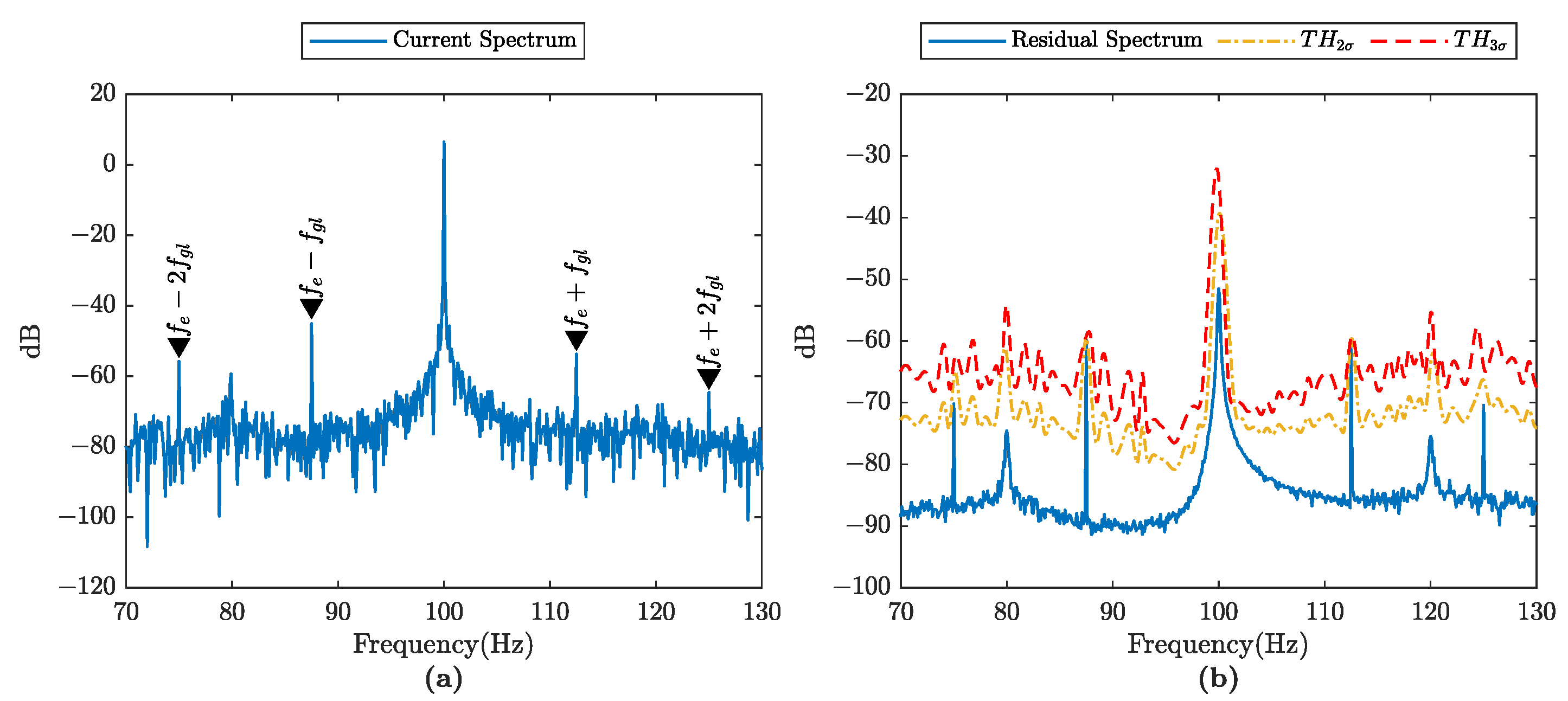
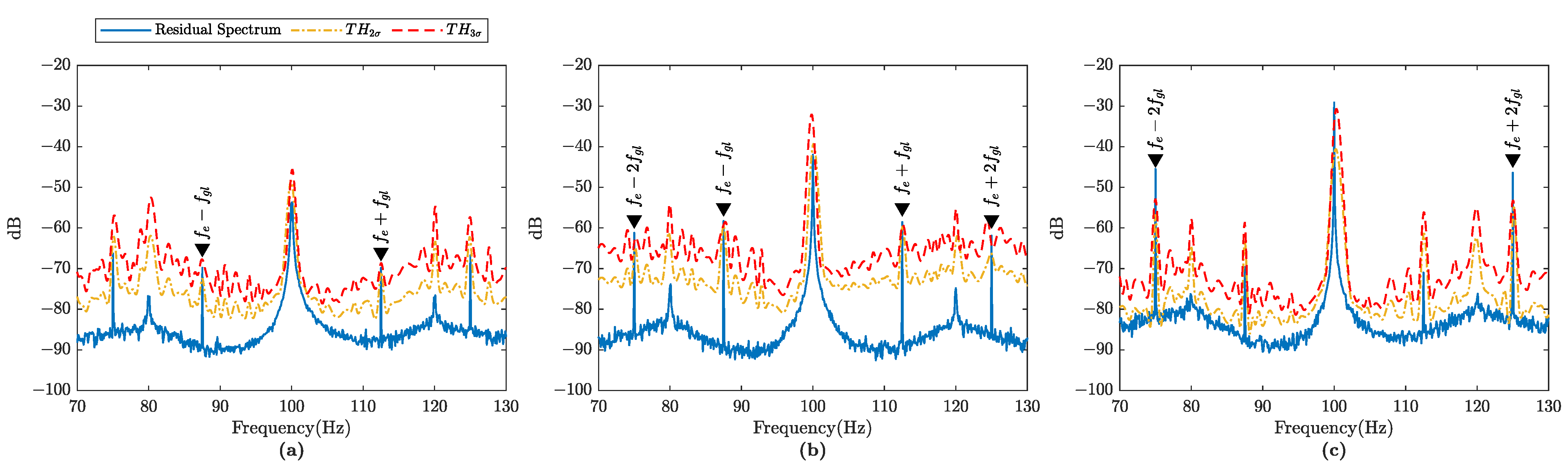
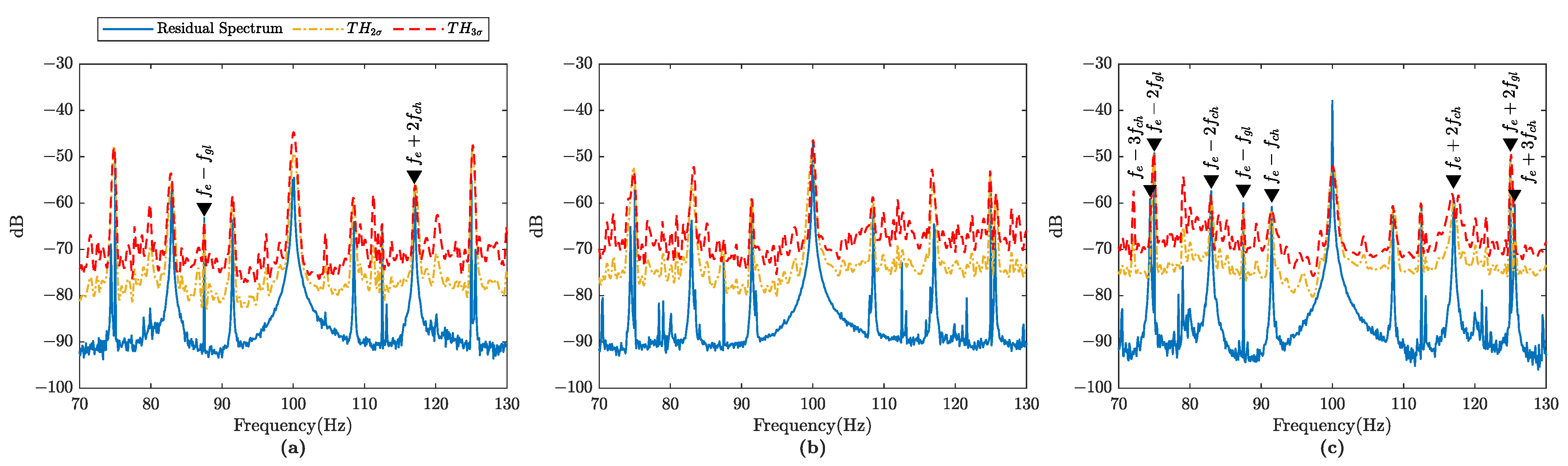
• The model-based FDI mitigates the influence from all the main harmonic frequencies that dominated the spectrum, thus leaving the fault frequencies in the residual current spectrum more visible. The fault frequencies magnitudes are evaluated using the residual current spectrum threshold without the need of expert knowledge. This approach has not been considered in MCSA before.
• A preliminary study to verify the model compatibility with the data in various load conditions.
• An indirect measurement approach for the transmission FDI. Most of the transmission FDIs are vibration-based that requires direct measurement in the transmission location. This approach is considered expensive and not always feasible in the cases where the vibration transducers cannot be installed at the designated location.

2. PMSM and Transmission Mathematical Models

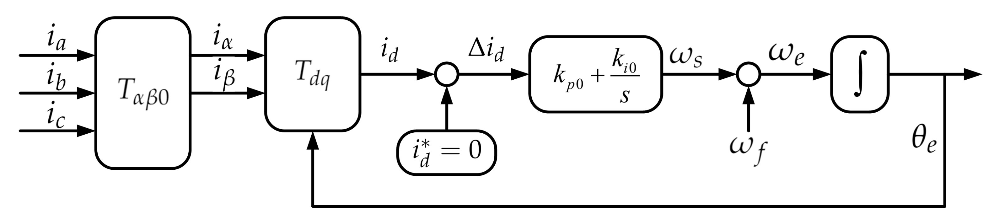
2.1. Coordinate Transformation

The stator-fixed three-phase $abc$-frame can be converted into the stator-fixed $\alpha \beta 0$-frame by using the following transformation matrix,

$$T_{\alpha \beta 0}=\frac{2}{3}\left[\begin{array}{ccc}1& -\frac{1}{2}& -\frac{1}{2}\\ 0& -\frac{\sqrt{3}}{2}& \frac{\sqrt{3}}{2}\\ \frac{1}{2}& \frac{1}{2}& \frac{1}{2}\end{array}\right]$$

(1)

Then, the stator-fixed $\alpha \beta 0$-frame can be converted into the synchronous $dq$-frame by using the following transformation matrix,

$$T_{dq}\left({\theta }_e\left(t\right)\right)=\left[\begin{array}{ccc}cos{\theta }_e\left(t\right)& -sin{\theta }_e\left(t\right)& 0\\ sin{\theta }_e\left(t\right)& cos{\theta }_e\left(t\right)& 0\\ 0& 0& 1\end{array}\right]$$

(2)

The stator-fixed three-phase $abc$-frame quantity can be reconstructed from the synchronous $dq$-frame quantity by using $T_{dq}{\left({\theta }_e\left(t\right)\right)}^{-1}$ and $T_{\alpha \beta 0}^{-1}$ matrices.

2.2. PMSM Differential Equation

In this study, an interior-type PMSM is used. Unlike the surface-type PMSM, the interior-type PMSM has a salient pole effect where the direct-axis inductance is not equal to the quadrature-axis inductance ($L_d\ne L_q$). The PMSM mathematical model can be expressed by the voltages and the flux linkages in the synchronous $dq$-frame as the following [13],

$$\begin{array}{cc}\hfill v_d& =R_s{i}_d+\frac{d}{dt}{\psi }_d-{\omega }_e{\psi }_q\hfill \\ \hfill v_q& =R_s{i}_q+\frac{d}{dt}{\psi }_q+{\omega }_e{\psi }_d\hfill \end{array}$$

(3)

$$\begin{array}{cc}\hfill {\psi }_d& =L_d{i}_d+{\psi }_m\hfill \\ \hfill {\psi }_q& =L_q{i}_q\hfill \end{array}$$

(4)

where $v_d$ and $v_q$ are the $dq$-frame voltages, $i_d$ and $i_q$ the $dq$-frame stator currents, $R_s$ is the stator resistance, ${\omega }_e$ is the electric angular velocity, ${\psi }_d$ and ${\psi }_q$ the $dq$-frame flux linkages, and ${\psi }_m$ is the mutual flux linkage. Substituting Equation (4) into (3), and as the permanent magnets are poor electrical conductors so that, $\frac{d}{dt}{\psi }_m=0$ [13], it yields

$$\begin{array}{cc}\hfill v_d& =R_s{i}_d+L_d\frac{d}{dt}{i}_d-{\omega }_e{L}_q{i}_q\hfill \\ \hfill v_q& =R_s{i}_q+L_q\frac{d}{dt}{i}_q+{\omega }_e(L_d{i}_d+{\psi }_m)\hfill \end{array}$$

(5)

In this study, the electric angular velocity ${\omega }_e$ can be easily obtained. Then, Equation (5) can be converted from the continuous-time domain into the discrete-time domain using the zero-order hold method as follows,

$$\left[\begin{array}{c}{i}_d(k+1)\\ i_q(k+1)\end{array}\right]=\left[\begin{array}{cc}-\frac{R_s}{L_d}{T}_s+1& \frac{{\omega }_e{L}_q}{L_d}{T}_s\\ -\frac{{\omega }_e{L}_d}{L_q}{T}_s& -\frac{R_s}{L_q}{T}_s+1\end{array}\right]\left[\begin{array}{c}{i}_d\left(k\right)\\ i_q\left(k\right)\end{array}\right]+\left[\begin{array}{cc}\frac{T_s}{L_d}& 0\\ 0& \frac{T_s}{L_q}\end{array}\right]\left[\begin{array}{c}{v}_d\left(k\right)\\ v_q\left(k\right)\end{array}\right]-\left[\begin{array}{c}0\\ \frac{{\omega }_e{\psi }_m}{L_q}{T}_s\end{array}\right]$$

(6)

where $T_s$ is the sampling time used to acquire the data.

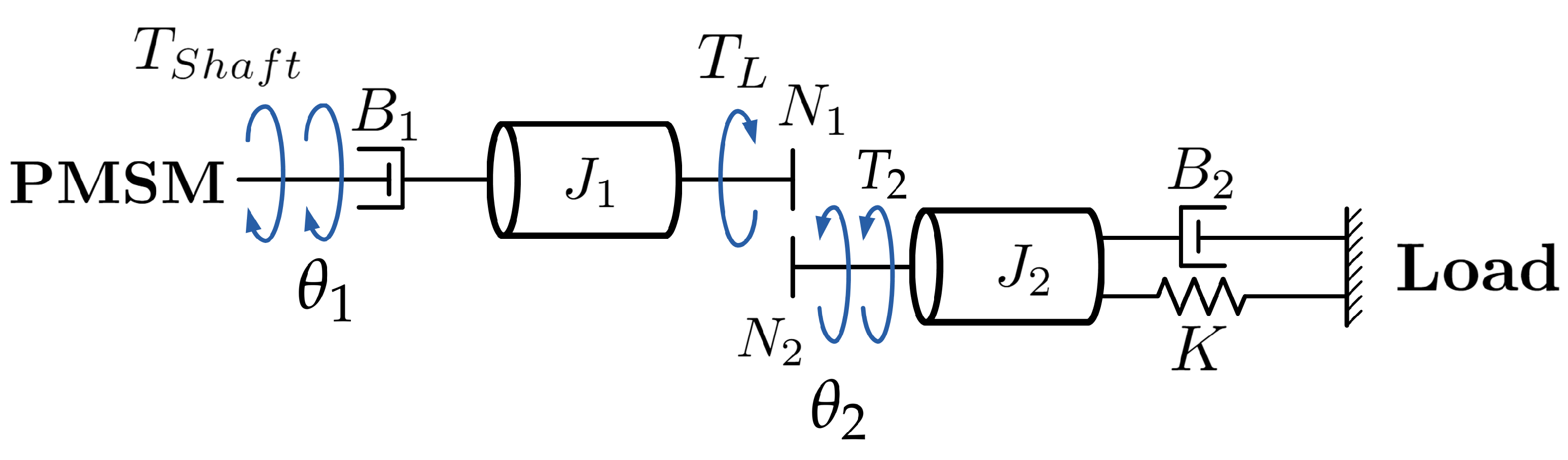
2.3. Transmission Model

This study proposes a general approximation of the mechanical transmission model instead of the fault transmission model. It is aimed to utilize this model to describe the dynamic input–output relationship of the inspected system for different transmission configurations and faults. Hence, the parameter deviation of the approximated model is observed instead of looking at the fault model structure as in general model-based FDI in this study. The mechanical transmission is approximated by using two mass–spring–damper systems, as shown in Figure 2. The gears are assumed ideal with no backlash. In Figure 2, the torques in the transmissions are derived as the following,

$$T_{Shaft}=J_1\frac{d^2}{d{t}^2}{\theta }_1+B_1\frac{d}{dt}{\theta }_1+T_L$$

(7)

$$T_L=T_2\frac{{\theta }_2}{{\theta }_1}=\frac{{\theta }_2}{{\theta }_1}(J_2\frac{d^2}{d{t}^2}{\theta }_2+B_2\frac{d}{dt}{\theta }_2+K{\theta }_2)=\frac{{\theta }_2^2}{{\theta }_1^2}(J_2\frac{d^2}{d{t}^2}{\theta }_1+B_2\frac{d}{dt}{\theta }_1+K{\theta }_1)$$

(8)

where $T_{Shaft}$ and $T_L$ are the shaft and the load torques, $J_1$ and $J_2$ are two gears’ inertia, respectively, $B_1$ and $B_2$ are the friction coefficients associated to each shaft, K is the spring coefficient at the load gear, and ${\theta }_1={\theta }_m$ is the rotor angular position. In addition, the ratio of the radii is inversely proportion to the ratio of the gear teeth number such that $\frac{{\theta }_2}{{\theta }_1}$ = $\frac{N_1}{N_2}$.

Substitute Equation (8) into (7) and replace the the ratio of the radii by the ratio of the gear teeth numberl; then, it arrives at,

$$T_{Shaft}=(J_1+J_2\frac{N_1^2}{N_2^2})\frac{d}{dt}{\omega }_m+(B_1+B_2\frac{N_1^2}{N_2^2}){\omega }_m+K\frac{N_1^2}{N_2^2}{\theta }_m$$

(9)

where ${\omega }_m=\frac{d}{dt}{\theta }_1$ is the rotor mechanical speed. Since the PMSM runs in a steady-state condition with constant speed and load, the $\frac{d}{dt}{\omega }_m=0$. Moreover, $T_{Shaft}$ is estimated through the linear relationship between the actual and the rated torque power as follows,

$$T_{Shaft}=\frac{T_{Rated}}{P_{Rated}}{P}_{In}$$

(10)

Then, by setting the $B_{GT}=B_1+B_2\frac{N_1^2}{N_2^2}$ and $K_{GT}=K\frac{N_1^2}{N_2^2}$, Equation (9) is simplified and is expressed in the discrete-time domain as the following,

$$T_{Shaft}\left(k\right)=B_{GT}{\omega }_m\left(k\right)+K_{GT}{\theta }_m\left(k\right)$$

(11)

Because the PMSM used in this study has four pole pairs, ${\omega }_m\left(k\right)$ and ${\theta }_m\left(k\right)$ are obtained by,

$$\begin{array}{ccc}\hfill {\omega }_m\left(k\right)=\frac{1}{4}{\omega }_e\left(k\right)& \hfill & \hfill {\theta }_m\left(k\right)=\frac{1}{4}{\theta }_e\left(k\right)\end{array}$$

(12)

where ${\omega }_e\left(k\right)$ and ${\theta }_e\left(k\right)$ are estimated through the Phase-Locked Loop (PLL), as shown in Figure 3. The lumped parameters $B_{GT}$ and $K_{GT}$ are therefore estimated through the relationship shown in Equation (11).

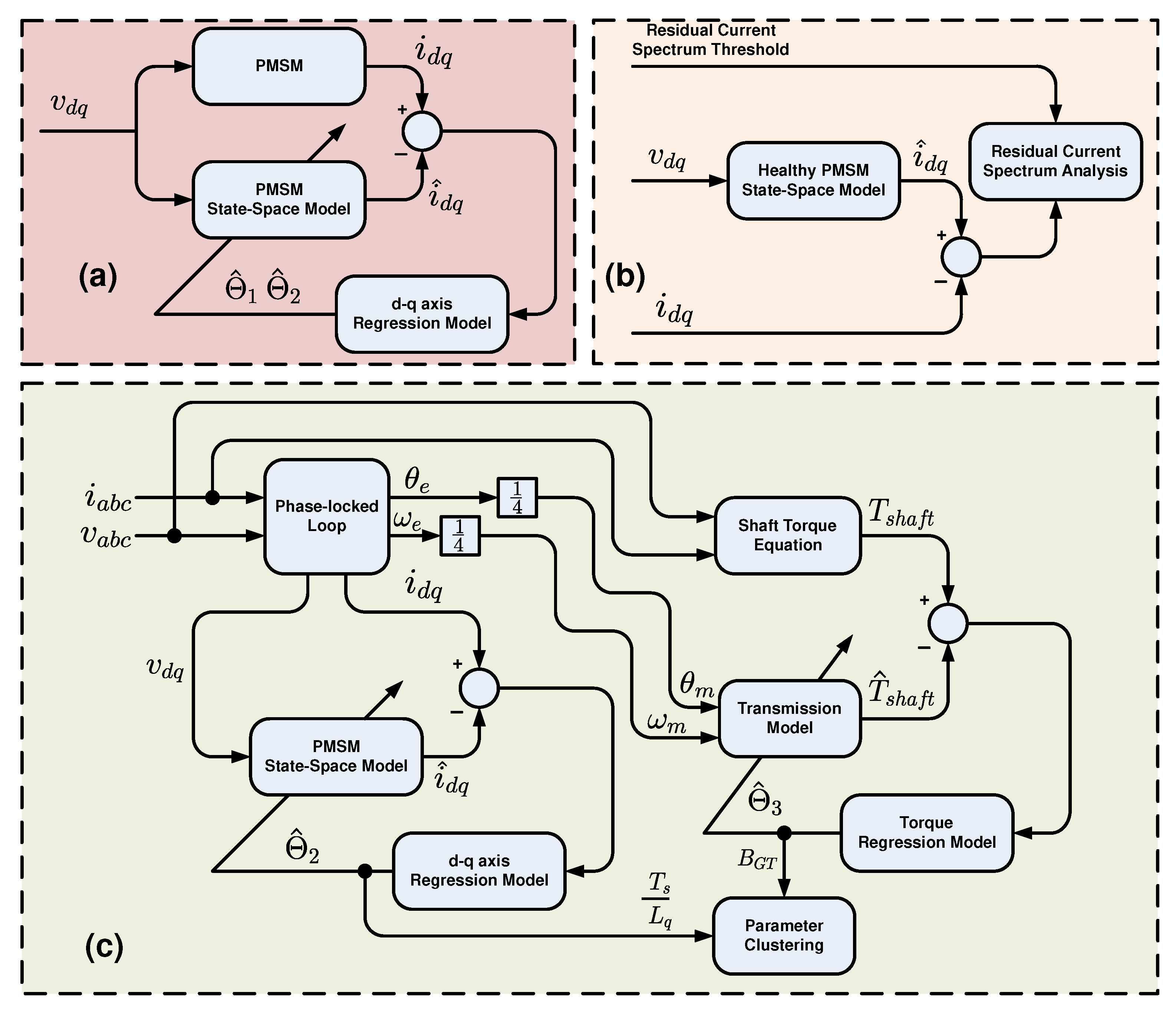
3. A Systematic Model-Based Fault Diagnosis Scheme

3.1. Parameter Estimation via Recursive Least Square

To estimate the model parameters of Equations (6) and (11) using the RLS algorithm, the models have to be arranged as the regression models first. Equation (6) can be divided into two regression models according to the d-axis and the q-axis as the following,

$$i_d(k+1)=\left[\begin{array}{ccc}{i}_q\left(k\right)& i_d\left(k\right)& v_d\left(k\right)\end{array}\right]\left[\begin{array}{c}\frac{{\omega }_e{L}_q}{L_d}{T}_s\\ -\frac{R_s}{L_d}{T}_s+1\\ \frac{T_s}{L_d}\end{array}\right]$$

(13)

$$i_q(k+1)=\left[\begin{array}{cccc}{i}_q\left(k\right)& i_d\left(k\right)& v_q\left(k\right)& {\omega }_e\end{array}\right]\left[\begin{array}{c}-\frac{R_s}{L_q}{T}_s+1\\ -\frac{{\omega }_e{L}_d}{L_q}{T}_s\\ \frac{T_s}{L_q}\\ -\frac{{\psi }_m}{L_q}{T}_s\end{array}\right]$$

(14)

Meanwhile, the torque regression model in Equation (11) can be described as follows,

$$T_{Shaft}\left(k\right)=\left[\begin{array}{cc}{\theta }_m\left(k\right)& {\omega }_m\left(k\right)\end{array}\right]\left[\begin{array}{c}{K}_{GT}\\ B_{GT}\end{array}\right]$$

(15)

In this study, the RLS algorithm will be implemented to estimate the parameters in Equations (13)–(15). Generally, the estimation problem can be defined as: using the dataset $\left\{\begin{array}{ccc}\left(x\left(k\right),y\left(k\right)\right)& |& k=1,2,\dots ,N\end{array}\right\}$and the RLS algorithm, estimate the parameters $\Theta$. The problem definition before performing the RLS algorithm is presented in

Table 1. The RLS algorithm problem definitions in this study.

Problems	Output	Input	Parameters
RLS 1 (Equation (13))	$y_1\left(k\right)=i_d(k+1)$	$x_1\left(k\right)=\left[\begin{array}{ccc}{i}_q\left(k\right)& i_d\left(k\right)& v_d\left(k\right)\end{array}\right]$	${\Theta }_1=\left[\begin{array}{c}\frac{{\omega }_e{L}_q}{L_d}{T}_s\\ -\frac{R_s}{L_d}{T}_s+1\\ \frac{T_s}{L_d}\end{array}\right]$
RLS 2 (Equation (14))	$y_2\left(k\right)=i_q(k+1)$	$x_2\left(k\right)=\left[\begin{array}{cccc}{i}_q\left(k\right)& i_d\left(k\right)& v_q\left(k\right)& {\omega }_e\end{array}\right]$	${\Theta }_2=\left[\begin{array}{c}-\frac{R_s}{L_q}{T}_s+1\\ -\frac{{\omega }_e{L}_d}{L_q}{T}_s\\ \frac{T_s}{L_q}\\ -\frac{{\psi }_m}{L_q}{T}_s\end{array}\right]$
RLS 3 (Equation (15))	$y_3\left(k\right)=T_{shaft}\left(k\right)$	$x_3\left(k\right)=\left[\begin{array}{cc}{\theta }_m\left(k\right)& {\omega }_m\left(k\right)\end{array}\right]$	${\Theta }_3=\left[\begin{array}{c}{K}_{GT}\\ B_{GT}\end{array}\right]$

.

The RLS algorithm to estimate the parameters $\widehat{\Theta }$ can be expressed as follows,

$${\widehat{\Theta }}_i(k+1)={\widehat{\Theta }}_i\left(k\right)+K(k+1)[y_i(k+1)-x_i(k+1){\widehat{\Theta }}_i\left(k\right)]$$

(16)

with

$$K(k+1)=P\left(k\right)x_i^T(k+1){[x_i(k+1)P\left(k\right)x_i^T(k+1)+W^{-1}]}^{-1}$$

(17)

$$P(k+1)=P\left(k\right)-K(k+1)x_i(k+1)P\left(k\right)$$

(18)

where subscript $i=1,2,3$ denotes the RLS algorithm problem definition in Table 1. The RLS algorithm procedures can be implemented as a pseudocode in Algorithm 1.

Algorithm 1 RLS algorithm

1: initialization: a dataset $\left\{\begin{array}{ccc}{x}_i\left(k\right),y_i\left(k\right)& |& k=1,2,\dots ,N\end{array}\right\}$; initial parameter $\widehat{\Theta }\left(0\right)$; weight W; and initial covariance matrix $P\left(0\right)$  2: for$k=0,1,2,3,\dots ,N-1$do  3:      $K(k+1)=P\left(k\right)x_i^T(k+1){[x_i(k+1)P\left(k\right)x_i^T(k+1)+W^{-1}]}^{-1}$  4:      $P(k+1)=P\left(k\right)-K(k+1)x_i(k+1)P\left(k\right)$  5:      ${\widehat{\Theta }}_i(k+1)={\widehat{\Theta }}_i\left(k\right)+K(k+1)[y_i(k+1)-x_i(k+1){\widehat{\Theta }}_i\left(k\right)]$  6: end for  7: The final estimated parameter is ${\widehat{\Theta }}_i\left(k\right)$ when the index $k=N$

3.2. Baseline Model and Residual Current Spectrum Threshold

A dataset of m measurements of the PMSM voltage and current signals in healthy condition is collected. Based on Figure 1a, the lumped parameters are estimated from the measured voltage and current signals. The procedure is presented in Algorithm 2 for loop lines 4 to 8. It requires Algorithm 1 to execute that for loop. After that, the identified lumped parameters are averaged to obtain a single value for each lumped parameter, as presented in Algorithm 2 line 10. The averaged lumped parameters are used to construct the baseline model using Equation (6). Then, a set of m residual current spectrum is generated using the baseline model from Algorithm 2. The residual current spectrum generation is presented in Algorithm 3 lines 3 to 9. It is important to note that in line 7, only the residual phase A is selected to generate the residual current spectrum threshold. It is not a requirement to use all the three phase residual current signals. A mean and a standard deviation are calculated from this set of residual current spectrum data. Finally, two different level thresholds are constructed from the residual current spectrum mean and the standard deviation data. The threshold construction is presented in Algorithm 3 lines 10 to 13.

Algorithm 2 Baseline model identification
1: initialization: m dataset $\left\{\begin{array}{ccc}{v}_d\left(k\right),v_q\left(k\right),i_d\left(k\right),i_q\left(k\right)& |& k=1,2,\dots ,N\end{array}\right\}$; and ${\omega }_e$;   2: set the problem definition of RLS 1 and RLS 2 as in Table 1   3: set matrix $\mathbf{H}=\mathrm{zeros}(7,m)$   4: for$j=1,2,3,\dots ,m$do   5:       estimate parameters ${\widehat{\Theta }}_1\in {\mathbb{R}}^{3\times 1}$ for RLS 1 via Algorithm 1   6:       estimate parameters ${\widehat{\Theta }}_2\in {\mathbb{R}}^{4\times 1}$ for RLS 2 via Algorithm 1   7:       update matrix $\mathbf{H}(:,j)=\left[\begin{array}{c}{\widehat{\Theta }}_1\\ {\widehat{\Theta }}_2\end{array}\right]$   8: end for   9: The final matrix $\mathbf{H}\in {\mathbb{R}}^{7\times m}$
10: calculate ${\Theta }_{mean}=\left[\begin{array}{c}\frac{1}{m}{\sum }_{j=1}^m\mathbf{H}(1,j)\\ ⋮\\ \frac{1}{m}{\sum }_{j=1}^m\mathbf{H}(7,j)\end{array}\right]\in {\mathbb{R}}^{7\times 1}$	▹ identified parameters mean
11: input ${\Theta }_{mean}$ as the parameters for Equation (6)	▹ PMSM baseline model

Algorithm 3 Residual current spectrum threshold development
1: initialization:m dataset $\left\{\begin{array}{ccc}{v}_d\left(k\right),v_q\left(k\right),i_d\left(k\right),i_q\left(k\right)& |& k=1,2,\dots ,N\end{array}\right\}$; ${\omega }_e$; and estimated parameters $\Theta$   2: set matrix $\mathbf{R}=\mathrm{zeros}(p,m)$   3: for$j=1,2,3,\dots ,m$do   4:       calculate $\left[\begin{array}{c}{\widehat{i}}_d\left(k\right)\\ {\widehat{i}}_q\left(k\right)\end{array}\right]$ using Equation (6) with parameters $\Theta$   5:       calculate $\left[\begin{array}{c}{r}_d\left(k\right)\\ r_q\left(k\right)\end{array}\right]=\left[\begin{array}{c}{i}_d\left(k\right)\\ i_q\left(k\right)\end{array}\right]-\left[\begin{array}{c}{\widehat{i}}_d\left(k\right)\\ {\widehat{i}}_q\left(k\right)\end{array}\right]$   6:       calculate $\left[\begin{array}{c}{r}_a\left(k\right)\\ r_b\left(k\right)\\ r_c\left(k\right)\end{array}\right]=T_{\alpha \beta 0}^{-1}{T}_{dq}{\left({\theta }_e\left(k\right)\right)}^{-1}\left[\begin{array}{c}{r}_d\left(k\right)\\ r_q\left(k\right)\\ 0\end{array}\right]$
7:       calculate $R_a\left(f\right)=\mathbf{fft}\left(r_a\left(k\right)\right)$ via FFT	▹ residual current spectrum
8:       update matrix $\mathbf{R}(:,j)=R_a\left(f\right)$   9: end for
10: calculate $\overline{R}=\left[\begin{array}{c}\frac{1}{m}{\sum }_{j=1}^m\mathbf{R}(1,j)\\ ⋮\\ \frac{1}{m}{\sum }_{j=1}^m\mathbf{R}(p,j)\end{array}\right]\in {\mathbb{R}}^{p\times 1}$	▹ residual current spectrum mean
11: calculate $R_{\sigma }=\left[\begin{array}{c}\sqrt{\frac{1}{m-1}{\sum }_{j=1}^m(\mathbf{R}(1,j)-{\overline{R}}_1)}\\ ⋮\\ \sqrt{\frac{1}{m-1}{\sum }_{j=1}^m(\mathbf{R}(1,j)-{\overline{R}}_p)}\end{array}\right]\in {\mathbb{R}}^{p\times 1}$	▹ residual current spectrum standard deviation
12: calculate $T{H}_{2\sigma }=\overline{R}+2\times R_{\sigma }$, where $T{H}_{2\sigma }\in {\mathbb{R}}^{p\times 1}$	▹$2\sigma$ threshold
13: calculate $T{H}_{3\sigma }=\overline{R}+3\times R_{\sigma }$, where $T{H}_{3\sigma }\in {\mathbb{R}}^{p\times 1}$	▹$3\sigma$ threshold

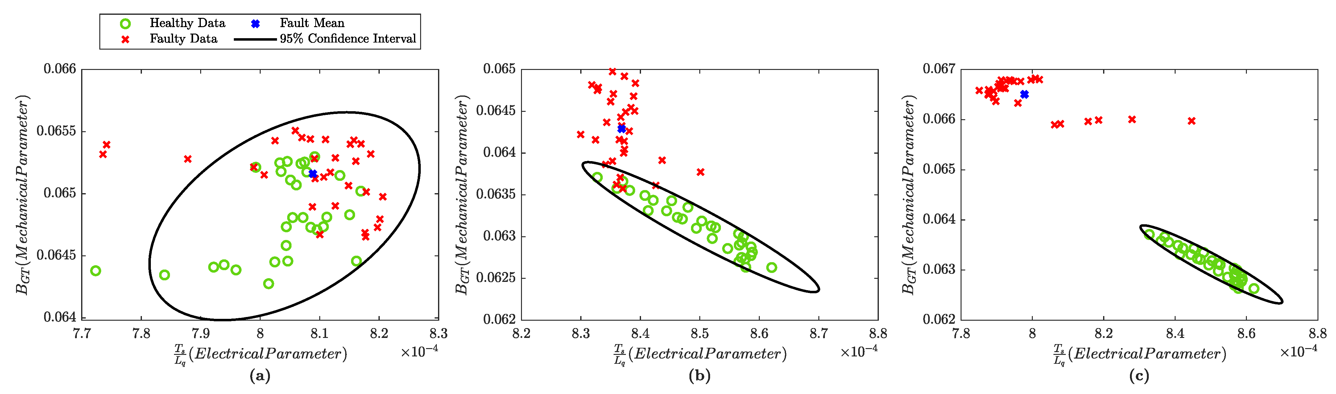
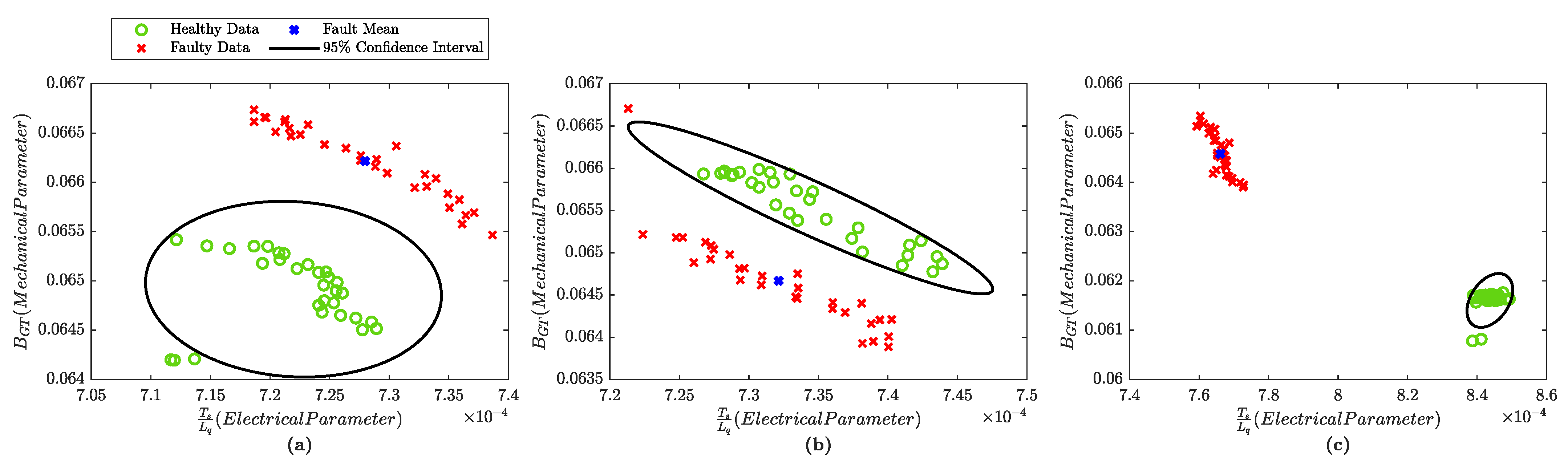
3.3. Parameter Clustering

In addition to the residual current spectrum analysis, the parameter clustering is included in the proposed PMSM transmission FDI, as shown in Figure 1c. According to Equations (13) to (15), there are in total nine lumped parameters that can be identified from the measured data. Considering that many of the true physical values are nontrivial to recover precisely due to the non-linearity, one electrical lumped parameter and one mechanical lumped parameter are chosen to form the parameter cluster. Because the d-axis is used as the reference in the synchronous $dq$-frame transformation, the d-axis current is zero. It is thus desirable to choose the lumped parameter that is unrelated to the d-axis. The electrical lumped parameter $\frac{T_s}{L_q}$ is chosen from Equation (14), and it is recovered trivially. Moreover, because the fault in transmission affects the friction coefficient, the mechanical lumped parameter $B_{GT}$ is chosen from Equation (15).

Firstly, a set of m healthy data is measured. The lumped parameters $\frac{T_s}{L_q}$ and $B_{GT}$ are estimated from this healthy dataset, as shown in Algorithm 4 lines 6 to 10. Finally, the parameter cluster plot is then generated. From this cluster plot, the 95% confidence range is calculated to generate the healthy condition boundary. This process is presented in Algorithm 4 lines 11 to 12. It is therefore that any condition will be considered faulty if the chosen parameter values are located outside the confidence span.

Algorithm 4 Healthy parameter confidence interval

1: initialization: m dataset $\left\{\begin{array}{ccc}{v}_a\left(k\right),v_b\left(k\right),v_c\left(k\right),i_a\left(k\right),i_b\left(k\right),i_c\left(k\right)& |& k=1,2,\dots ,N\end{array}\right\}$; This dataset is obtained from a normal condition PMSM   2: obtain ${\omega }_e$ and ${\theta }_e$ using PLL, then, calculate ${\omega }_m=\frac{1}{4}{\omega }_e$, and ${\theta }_m=\frac{1}{4}{\theta }_e$   3: calculate $T_{Shaft}=\frac{T_{Rated}}{P_{Rated}}{P}_{In}$   4: calculate $\left[\begin{array}{c}{i}_d\left(k\right)\\ i_q\left(k\right)\\ i_0\left(k\right)\end{array}\right]=T_{dq}\left({\theta }_e\left(k\right)\right)T_{\alpha \beta 0}\left[\begin{array}{c}{i}_a\left(k\right)\\ i_b\left(k\right)\\ i_c\left(k\right)\end{array}\right]$, and $\left[\begin{array}{c}{v}_d\left(k\right)\\ v_q\left(k\right)\\ v_0\left(k\right)\end{array}\right]=T_{dq}\left({\theta }_e\left(k\right)\right)T_{\alpha \beta 0}\left[\begin{array}{c}{v}_a\left(k\right)\\ v_b\left(k\right)\\ v_c\left(k\right)\end{array}\right]$   5: set the problem definition of RLS 2 and RLS 3 as in Table 1   6: for$j=1,2,3,\dots ,m$do   7:       estimate parameters ${\widehat{\Theta }}_2\in {\mathbb{R}}^{4\times 1}$ for RLS 2 via Algorithm 1   8:       estimate parameters ${\widehat{\Theta }}_3\in {\mathbb{R}}^{2\times 1}$ for RLS 3 via Algorithm 1   9:       get $\frac{T_s}{L_q}$ from ${\widehat{\Theta }}_2(3,j)$, and $B_{GT}$ from ${\widehat{\Theta }}_3(2,j)$  10: end for  11: create cluster plot via scatter($\frac{T_s}{L_q}$,$B_{GT}$)  12: calculate the 95% confidence interval of healthy cluster plot

3.4. Fault Characteristic Frequency Detection

A short periodic impulse occurs in the current signal whenever the driving gear comes in contact with a damaged tooth in the driven gear. The impulse is modulated around the fundamental frequency and generates the side-band harmonics [27]. The driving gear fault characteristic frequency $f_m$ is expressed as the following,

$$\begin{array}{cc}\hfill f_{gm}& =\frac{f_e}{n_p}\hfill \\ \hfill f_m& =f_e\pm k{f}_{gm}\hfill \end{array}$$

(19)

where $f_e$ is the operational frequency and $n_p$ is the number of the PMSM pole, and $k=1,2,\dots$. Since there is a changing ratio between the driving and the driven gears, the gear ratio $g_r$ is considered in the driven gear fault characteristic frequency $f_l$ calculation as depicted in the following,

$$\begin{array}{cc}\hfill f_{gl}& =\frac{f_e}{g_r{n}_p}\hfill \\ \hfill f_l& =f_e\pm k{f}_{gl}\hfill \end{array}$$

(20)

In contrast to the gear-to-gear direct contacting configuration, the sprocket–chain configuration has a series chain connecting the driving and the driven sprockets. The literature rarely studies the sprocket–chain transmission fault. On the other hand, the sprocket–chain transmission has a similar mechanical configuration as the belt–pulley transmission. Thus, the chain fault characteristic frequency is depicted based on the belt fault characteristic frequency as following [28],

$$f_{ch}=\frac{2\pi r_m{f}_r}{l_{ch}}$$

(21)

where $f_r$ is the driving gear rotation frequency, $r_m$ is the driving gear radius, and $l_{ch}$ is the chain length. Due to the similar physical phenomena to the gear set, the sprocket fault characteristic frequency in the spectrum is described using the formula from the gear fault characteristic frequency,

$$f_{sc}=f_e\pm k{f}_{ch}$$

(22)

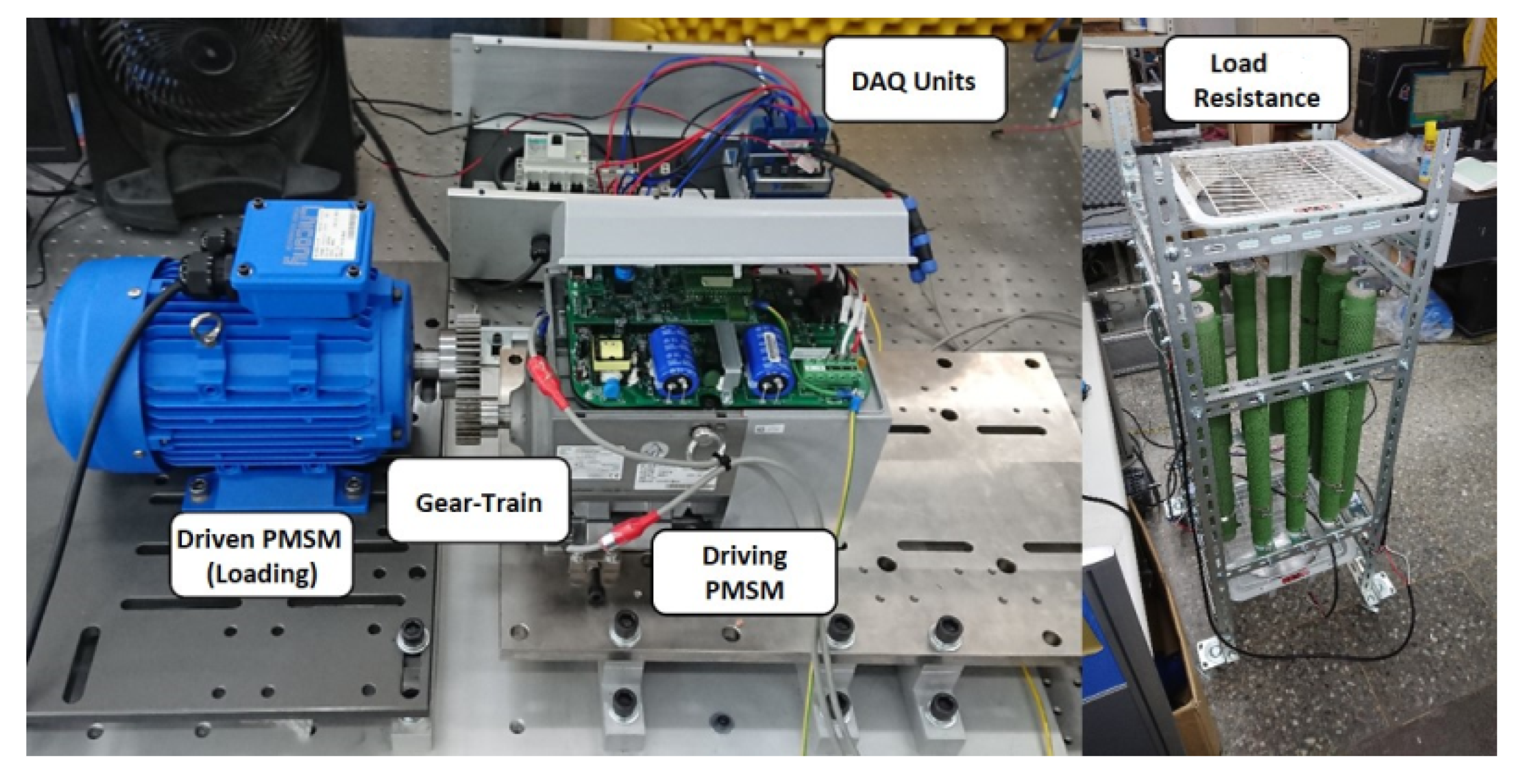
4. Experimental Setup

4.1. PMSM Load Experimental Platform

The driving motor used in this study is a Chicony PMSM. The PMSM motor has a built-in variable frequency drive with a closed-loop speed controller. Another Chicony PMSM without an inverter is configured as a driven motor on the load side. The driven motor is connected to the electrical load resistance and serves as a generator to simulate various operation load conditions. In this study, the driving PMSM is operated in 100 Hz operation frequency and reaches 80% load condition by changing the load resistance value, as shown in Figure 4. The driving and the driven motors’ rated specifications are shown in

Table 2. Driving and driven PMSM rated specifications.

Parameters	Driving PMSM	Driven PMSM	Units
Rated Voltage	380	380	Volt
Rated Current	6.6	8.3	Amp
Rated Power	2.2	3.7	kW
Rated Speed	1500	1500	RPM
Rated Torque	14	23.6	Nm
Poles	4	4	pair
Efficiency	89.4	91.9	%

. The signal data acquisition process is accomplished by using a 24-bits NI-9244 card for the three-phase voltage signal acquisition and a 24-bits NI-9239 card for the three-phase current signal acquisition. The NI data acquisition cards are set at a 25 kHz sampling frequency. The data acquisition interface is programmed using the NI LabVIEW.

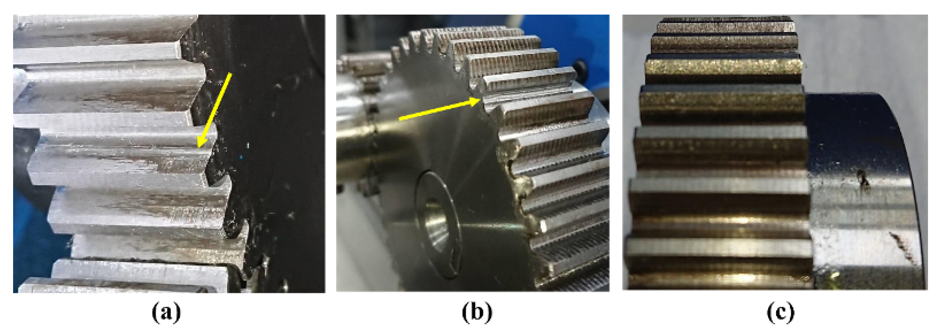
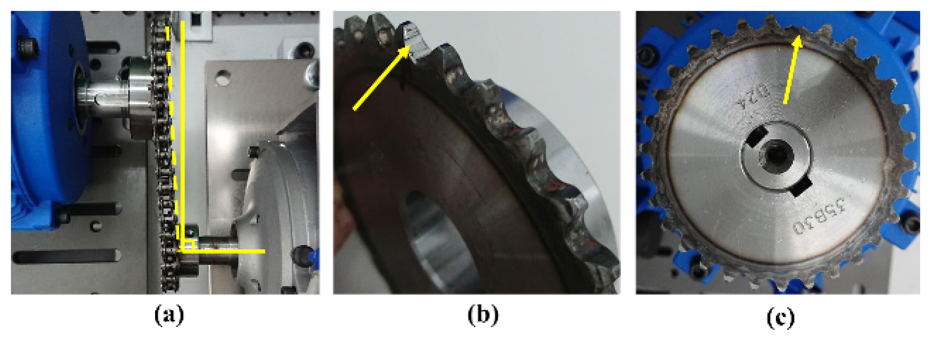
4.2. Transmission Faulty Specimens

The faults in two types of transmission configuration, being gear-to-gear and sprocket–chain, are experimented. As shown in Figure 5, three fault conditions have been tested for the gear-to-gear transmission, including slight wear at one of the driven gear teeth, severe wear along the surface on one of the driven gear tooth, and no lubricant condition. For the sprocket–chain configuration shown in Figure 6, three experimented fault conditions are slight wear at one of the driven gear teeth, one missing tooth at the driven gear, and chain alignment offset from the driving gear to the driven gear. The gear specifications for the gear-to-gear and the sprocket–chain are listed in

Table 3. Gear-to-gear and sprocket–chain specifications.

		Driving Gear	Driven Gear	Units
gear-to-gear	No. teeth	20	40	-
	Pressure angle	20	20	${}^{\circ }$
	Gear module	2	2	-
sprocket–chain	No. teeth	15	30	-
	Pitch circle diameter	45.81	91.12	mm
	Chain length	423		mm

. According to Table 3, the gear-to-gear ratio and the sprocket–chain ratio between the driving and the driven gears are 1:2. In the fault experiments, the PMSM load is fixed at 80%.

5. Results and Discussions

5.1. Fault Detection and Identification

The current spectrum of PMSM with the gear-to-gear transmission under healthy condition is shown in Figure 7a. Certain side-bands are observed and verified to be related to the driven gear characteristic frequency $f_e\pm k{f}_{gl}$. The presence of these feature frequencies in the current spectrum is reasonable because of the dynamic interaction between two gears and the inevitable tolerance in the gear manufacturing. Due to the lack of fault threshold standard in MCSA, an intuitive evaluation on this current spectrum may lead to a false diagnosis of the gear-to-gear transmission condition. Therefore, the model-based approach is proposed and implemented in this study, and a residual current spectrum is obtained for the purpose of FDI, as shown in Figure 7b. The residual current spectrum threshold for healthy data is obtained by using Algorithm 3, and the residual current spectrum is evaluated based on its standard deviation. From the observation of Figure 7b, the driven gear characteristic frequency $f_e\pm k{f}_{gl}$ is less than the 2 standard deviation threshold ($T{H}_{2\sigma }$). Thus, it implies a healthy condition. A more detailed comparison between MCSA and the model-based approach for electric motor fault diagnosis can be found in [21].

Three different fault conditions are experimented for gear-to-gear transmission, as shown in Figure 5, and their residual current spectrum result is presented in Figure 8. Figure 8a shows the residual current spectrum of a slightly worn fault in one of the driven gear teeth. It can be seen that $f_e\pm k{f}_{gl}$ at 87.5 Hz and 112.5 Hz have amplitudes higher than $T{H}_{2\sigma }$ but below $T{H}_{3\sigma }$. In comparison to the slightly worn fault, peaks at $f_e\pm k{f}_{gl}$ at 75 Hz, 87.5 Hz, 112.5 Hz, and 125 Hz have amplitudes higher than $T{H}_{3\sigma }$ for the severely worn fault, as shown in Figure 8b. In no lubricant fault, the signature peak of $f_e\pm k{f}_{gl}$ has a higher peak than the $T{H}_{3\sigma }$ at 75 Hz and 125 Hz, as seen in Figure 8c.

As shown in Figure 1, the proposed FDI scheme also includes parameters clustering. For all gear-to-gear fault cases, a comparison of identified lumped parameter values between 30 healthy and 30 fault data is demonstrated. From the set of 30 healthy data, a 95% confidence span of parameter cluster is generated using Algorithm 4. As shown in Figure 9, the identified lumped parameter values from healthy data are represented as the green circles, and the faulty data values are represented as the red crosses. For the slightly worn driven-gear fault, the faulty parameter cluster almost overlaps the healthy confidence span, as seen in Figure 9a. It implies that the slight wear damage is not severe enough and just incipient. Thus, it could not be detected using the parameter clustering. This is also confirmed by the residual current spectrum, as the $f_e\pm k{f}_{gl}$ amplitudes are higher than $T{H}_{2\sigma }$ but lower than $T{H}_{3\sigma }$. For the severely worn fault in Figure 9b, it is observed that the faulty parameter cluster lies almost outside of the healthy confidence span. Moreover, for the no-lubricant case in Figure 9c, the faulty parameter cluster is located in a distinct distance outside the healthy confidence span. Since there is no lubricant in both the driving and the driven gears, the friction force between these gears has increased. As a result, the friction-related parameter is identified as higher than that in the healthy condition. The friction-related parameter $B_{GT}$ causes the distinct distance between the healthy and faulty parameter clusters in Figure 9c.

The conditions for the three different sprocket–chain faults are shown in Figure 6. The residual current spectrum result of the chain offset fault is shown in Figure 10a. The fault signature of $f_e\pm k{f}_{gl}$ has a peak higher than $T{H}_{3\sigma }$ at 87.5 Hz and also a peak of $f_e\pm k{f}_{ch}$ higher than $T{H}_{3\sigma }$ at 117 Hz, as seen in Figure 10a. The residual current spectrum of a slightly worn fault in the sprocket shows no clear signature that is higher than $T{H}_{2\sigma }$ or $T{H}_{3\sigma }$, as seen in Figure 10b. The slightly worn fault is considered incipient to generate a signature amplitude higher than the threshold in the experiment. On the other hand, in the case of one missing tooth, the residual current spectrum shows that the signature of $f_e\pm k{f}_{gl}$ has peaks higher than $T{H}_{3\sigma }$ at 75 Hz, 87.5 Hz, and 125 Hz, as seen in Figure 10c. It is also observed that the peaks of signature $f_e\pm k{f}_{ch}$ are higher than $T{H}_{3\sigma }$ at 74.4 Hz, 83 Hz, 91.5 Hz, 117 Hz, and 125.6 Hz.

Based on Figure 11a, the parameter cluster of the chain offset fault lies outside of the healthy confidence span. A similar phenomenon also happened to the slightly worn tooth and one missing tooth faults. The parameter cluster lies outside the healthy confidence span for both faults, as shown in Figure 11b,c. As seen from the residual current spectrum for the slightly worn faults, the signature peaks are low in the magnitude as well. The same information is also concluded using the parameter clustering, as the distance between the faulty parameter cluster and the healthy confidence span is closer. However, the faulty parameter cluster lies outside the healthy confidence span. Meanwhile, the missing tooth case is severe enough to establish a distinguishable distance of the fault parameter cluster. In the case that the sprocket–chain fault is incipient and the residual current spectrum fails to detect the this fault, the parameter clustering approach provides better sensitivity to detect the fault because the identified mechanical related parameter $B_{GT}$ is strongly linked to the friction coefficient.

Table 4. The summary of gear-to-gear and sprocket–chain transmissions FDI results using residual current spectrum threshold and parameter cluster.

Transmission	Fault	Load	Residual Current Spectrum	Parameter Cluster
gear-to-gear	slightly worn	80%	caution	normal
	severely worn	80%	warning	warning
	no lubricant	80%	warning	warning
sprocket–chain	chain offset	80%	warning	warning
	slightly worn	80%	normal	warning
	one missing tooth	80%	warning	warning

shows the summary of the FDI results for the experimented gear-to-gear and sprocket–chain faults. In the residual current spectrum, the warning is above the $T{H}_{3\sigma }$, and the caution is above the $T{H}_{2\sigma }$ but below the $T{H}_{3\sigma }$. In the parameter cluster, the warning means that the fault parameter cluster lies outside the healthy confidence span. It can be observed that the combination of the residual current spectrum threshold and the parameter cluster helps to define the FDI decision confidently. For example, in the case of slightly worn faults in gear-to-gear where the damage is incipient, the parameter cluster fails but the residual current spectrum shows a caution alarm. In the case of a slightly worn fault in the sprocket–chain where the damage is incipient, the residual current spectrum threshold fails but the parameter cluster shows a warning alarm. When the damage is severe enough, both the residual current spectrum threshold and parameter cluster show the same warning alarm.

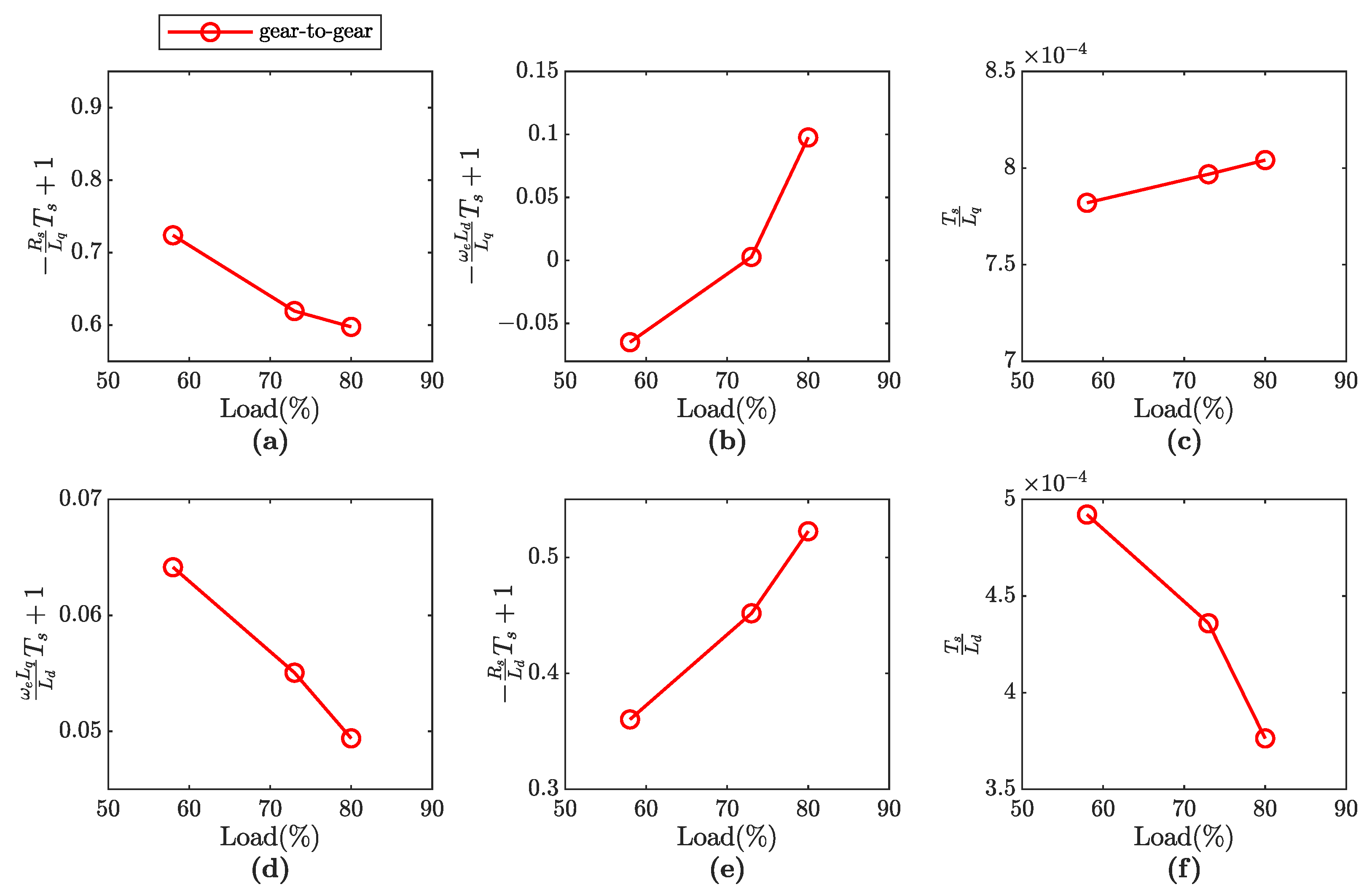
5.2. Load Variations

The PMSM operating condition discussed in this study is a steady-state condition with constant operating speed and load. In this case, the PMSM is assumed to be a linear time-invariant system, as shown in Equation (6). However, the parameters presented in Equation (6) indeed vary with different operating conditions. It is observed from Figure 12 where the lumped parameter values of the PMSM for three different load conditions are identified. The lumped parameter values are presented in 58%, 73%, and 80% load conditions. This load change is done by adjusting the resistance value of the variable resistors in Figure 4. During the load change, the PMSM operating speed is kept constant at 1500 RPM.

It is observed that all the PMSM model lumped parameters vary according to the load conditions in Figure 12. Therefore, a specific parameter set identified under a particular load condition should only be used in the model to represent that specific load condition.

Table 5. Residual RMSE comparison of gear-to-gear transmission measured signal and estimated signal based on the load conditions.

	58% Load Estimated Signal	73% Load Estimated Signal	80% Load Estimated Signal
58% Load Measured Signal	2.77%	5.73%	7.85%
73% Load Measured Signal	7.32%	2.11%	4.18%
80% Load Measured Signal	16.76%	5.58%	1.90%

shows the residual fitting error between the measured signal and the estimated signal at particular load conditions. If the fitting residual error is small, it implies that the model is proper to describe those load conditions. This result demonstrates that a proper model must be cautiously selected according to the operation condition. In a broad sense, the selection is applied to the model and the residual current spectrum threshold. The residual current spectrum threshold must be determined for a specific load condition using a specific model identified under that load. Thus, the solution presented in this study is limited only to a steady-state operating condition. The future development will be carried out for transient and more dynamic operating conditions.

6. Conclusions

For a PMSM with mechanical transmission, the transmission fault characteristic frequencies in the current spectrum are inevitable due to the dynamic interaction between two or more gears and sprockets. The conventional MCSA may lead to false diagnosis due to its lack of fault magnitude threshold standards. Through the residual current spectrum threshold, the fault characteristic frequencies magnitude is easily evaluated. The fault detection can also be accomplished through the parameter value monitoring. Combining electrical and mechanical lumped parameters, these parameters are visualized as a cluster to differentiate the normal and the faulty conditions. Three different fault conditions are experimented for gear-to-gear and sprocket–chain transmissions to evaluate the proposed method. The results demonstrate that the combination of the residual current spectrum threshold and the parameter cluster can be used for fault diagnosis decisions and has achieved satisfactory results.

This study is limited to the steady-state conditions with constant speed and load. Based on the presented results, the estimated model parameters will also change as the load conditions change. Thus, for PMSMs with the transient conditions where the operating condition is varying in a short time, this solution may not be applicable. However, this study still provides insights especially in regard to the sensitivity compared to MCSA and the load influence, and it can be used as a reference in developing the model-based FDI for PMSM in transient conditions. In the future, the PMSM will be operated in different operating frequencies and loads. A set of the healthy state-space model and the residual current spectrum threshold will be identified and generated for each combination of the operating frequency and load. Then, the set of the state-space and the current spectrum residual threshold will be selected based on the operating frequency and load of the data utilized. This approach is similar to the gain scheduling in the adaptive control method.

References

1. Mohanty, A.; Kar, C. Fault Detection in a Multistage Gearbox by Demodulation of Motor Current Waveform. IEEE Trans. Ind. Electron. 2006, 53, 1285–1297. [Google Scholar] [CrossRef]
2. Yuan, X.; Cai, L. Variable amplitude Fourier series with its application in gearbox diagnosis—Part I: Principle and simulation. Mech. Syst. Signal Process. 2005, 19, 1055–1066. [Google Scholar] [CrossRef]
3. Wang, X.; Makis, V.; Yang, M. A wavelet approach to fault diagnosis of a gearbox under varying load conditions. J. Sound Vib. 2010, 329, 1570–1585. [Google Scholar] [CrossRef]
4. Chen, X.; Feng, Z. Time-Frequency Analysis of Torsional Vibration Signals in Resonance Region for Planetary Gearbox Fault Diagnosis Under Variable Speed Conditions. IEEE Access 2017, 5, 21918–21926. [Google Scholar] [CrossRef]
5. Zak, G.; Wylomanska, A.; Zimroz, R. Local Damage Detection Method Based on Distribution Distances Applied to Time-Frequency Map of Vibration Signal. IEEE Trans. Ind. Appl. 2018, 54, 4091–4103. [Google Scholar] [CrossRef]
6. Jung, J.; Lee, S.B.; Lim, C.; Cho, C.H.; Kim, K. Electrical Monitoring of Mechanical Looseness for Induction Motors With Sleeve Bearings. IEEE Trans. Energy Convers. 2016, 31, 1377–1386. [Google Scholar] [CrossRef]
7. Kia, S.; Henao, H.; Capolino, G.A. Analytical and Experimental Study of Gearbox Mechanical Effect on the Induction Machine Stator Current Signature. IEEE Trans. Ind. Appl. 2009, 45, 1405–1415. [Google Scholar] [CrossRef]
8. Purbowaskito, W.; Lan, C.Y.; Liu, M.K.; Fuh, K. A Novel Scheme on Fault Diagnosis of Induction Motors using Current per Voltage Bode Diagram. J. Chin. Soc. Mech. Eng. 2020, 41, 781–790. [Google Scholar]
9. Zhang, R.; Gu, F.; Mansaf, H.; Wang, T.; Ball, A.D. Gear wear monitoring by modulation signal bispectrum based on motor current signal analysis. Mech. Syst. Signal Process. 2017, 94, 202–213. [Google Scholar] [CrossRef]
10. ISO 20958:2013; Condition monitoring and diagnostics of machine systems—Electrical signature analysis of three-phase induction motors. Standard, International Organization for Standardization: Geneva, Switzerland, 2013.
11. Chen, J.; Yang, F. Data-driven subspace-based adaptive fault detection for solar power generation systems. IET Contr. Theory Appl. 2013, 7, 1498–1508. [Google Scholar] [CrossRef]
12. Dai, X.; Gao, Z. From Model, Signal to Knowledge: A Data-Driven Perspective of Fault Detection and Diagnosis. IEEE Trans. Ind. Informatics 2013, 9, 2226–2238. [Google Scholar] [CrossRef] [Green Version]
13. Krause, P.; Wasynczuk, O.; Sudhoff, S.; Pekarek, S. (Eds.) Analysis of Electric Machinery and Drive Systems; John Wiley & Sons, Inc.: Hoboken, NJ, USA, 2013. [Google Scholar] [CrossRef]
14. Mazzoletti, M.A.; Bossio, G.R.; Angelo, C.H.D.; Espinoza-Trejo, D.R. A Model-Based Strategy for Interturn Short-Circuit Fault Diagnosis in PMSM. IEEE Trans. Ind. Electron. 2017, 64, 7218–7228. [Google Scholar] [CrossRef]
15. Kiselev, A.; Kuznietsov, A.; Leidhold, R. Model based online detection of inter-turn short circuit faults in PMSM drives under non-stationary conditions. In Proceedings of the 2017 11th IEEE International Conference on Compatibility, Power Electronics and Power Engineering, Cadiz, Spain, 4–6 April 2017. [Google Scholar] [CrossRef]
16. Zhan, H.; Zhu, Z.Q.; Odavic, M.; Li, Y. A Novel Zero-Sequence Model-Based Sensorless Method for Open-Winding PMSM With Common DC Bus. IEEE Trans. Ind. Electron. 2016, 63, 6777–6789. [Google Scholar] [CrossRef]
17. Hang, J.; Zhang, J.; Ding, S.; Huang, Y.; Wang, Q. A Model-Based Strategy With Robust Parameter Mismatch for Online HRC Diagnosis and Location in PMSM Drive System. IEEE Trans. Power Electron. 2020, 35, 10917–10929. [Google Scholar] [CrossRef]
18. Kommuri, S.K.; Defoort, M.; Karimi, H.R.; Veluvolu, K.C. A Robust Observer-Based Sensor Fault-Tolerant Control for PMSM in Electric Vehicles. IEEE Trans. Ind. Electron. 2016, 63, 7671–7681. [Google Scholar] [CrossRef]
19. Zhang, J.; Yao, H.; Rizzoni, G. Fault Diagnosis for Electric Drive Systems of Electrified Vehicles Based on Structural Analysis. IEEE Trans. Veh. Technol. 2017, 66, 1027–1039. [Google Scholar] [CrossRef]
20. Overschee, P.V.; Moor, B.D. Subspace Identification for Linear Systems; Kluwer Academic: Dordrecht, The Netherlands, 1996. [Google Scholar] [CrossRef]
21. Purbowaskito, W.; Lan, C.Y.; Fuh, K. A Novel Fault Detection and Identification Framework for Rotating Machinery Using Residual Current Spectrum. Sensors 2021, 21, 5865. [Google Scholar] [CrossRef]
22. Tariq, M.F.; Khan, A.Q.; Abid, M.; Mustafa, G. Data-Driven Robust Fault Detection and Isolation of Three-Phase Induction Motor. IEEE Trans. Ind. Electron. 2019, 66, 4707–4715. [Google Scholar] [CrossRef]
23. Brosch, A.; Hanke, S.; Wallscheid, O.; Bocker, J. Data-Driven Recursive Least Squares Estimation for Model Predictive Current Control of Permanent Magnet Synchronous Motors. IEEE Trans. Power Electron. 2021, 36, 2179–2190. [Google Scholar] [CrossRef]
24. Vahidi, A.; Stefanopoulou, A.; Peng, H. Recursive least squares with forgetting for online estimation of vehicle mass and road grade: Theory and experiments. Veh. Syst. Dyn. 2005, 43, 31–55. [Google Scholar] [CrossRef]
25. Kuen, H.Y.; Mjalli, F.S.; Koon, Y.H. Recursive Least Squares-Based Adaptive Control of a Biodiesel Transesterification Reactor. Ind. Eng. Chem. Res. 2010, 49, 11434–11442. [Google Scholar] [CrossRef]
26. Souza, D.A.D.; Batista, J.G.; Vasconcelos, F.J.S.; Reis, L.L.N.D.; Machado, G.F.; Costa, J.R.; Junior, J.N.N.; Silva, J.L.N.; Rios, C.S.N.; Junior, A.B.S. Identification by Recursive Least Squares With Kalman Filter (RLS-KF) Applied to a Robotic Manipulator. IEEE Access 2021, 9, 63779–63789. [Google Scholar] [CrossRef]
27. Rajagopalan, S.; Habetler, T.G.; Harley, R.G.; Sebastian, T.; Lequesne, B. Current/Voltage-Based Detection of Faults in Gears Coupled to Electric Motors. IEEE Trans. Ind. Appl. 2006, 42, 1412–1420. [Google Scholar] [CrossRef]
28. Kang, T.J.; Yang, C.; Park, Y.; Hyun, D.; Lee, S.B.; Teska, M. Electrical Monitoring of Mechanical Defects in Induction Motor-Driven V-Belt–Pulley Speed Reduction Couplings. IEEE Trans. Ind. Appl. 2018, 54, 2255–2264. [Google Scholar] [CrossRef]
Figure 1. PMSM model-based fault detection and identification: (a) healthy PMSM model identification; (b) residual current spectrum analysis; (c) parameter clustering.
Electronics 11 01356 g001
Figure 2. Mass–spring–damper approximation model for transmission.
Electronics 11 01356 g002
Figure 3. PLL block diagram.
Electronics 11 01356 g003
Figure 4. PMSM load experimental platform.
Electronics 11 01356 g004
Figure 5. Gear-to-gear faults: (a) slightly worn damage at a tooth of the driven gear; (b) severely worn damage along a tooth of the driven gear; (c) no lubricant at both the driving and driven gear.
Electronics 11 01356 g005
Figure 6. Sprocket–chain faults: (a) chain offset from the driving gear to the driven gear; (b) slightly worn damage at a tooth of the driven gear; (c) one missing tooth of the driven gear.
Electronics 11 01356 g006
Figure 7. Gear-to-gear spectrum: (a) motor current spectrum; (b) residual current spectrum.
Electronics 11 01356 g007
Figure 8. Gear-to-gear fault residual current spectrum: (a) slightly worn damage at a tooth of the driven gear; (b) severely worn damage along a tooth of the driven gear; (c) no lubricant at both the driving and driven gear.
Electronics 11 01356 g008
Figure 9. Gear-to-gear fault parameter clustering: (a) slightly worn damage at a tooth of the driven gear; (b) severely worn damage along a tooth of the driven gear; (c) no lubricant at both the driving and driven gear.
Electronics 11 01356 g009
Figure 10. Sprocket–chain fault residual current spectrum: (a) chain offset from the driving gear to the driven gear; (b) slightly worn damage at a tooth of the driven gear; (c) one missing tooth of the driven gear.
Electronics 11 01356 g010
Figure 11. Sprocket–chain fault parameter clustering: (a) chain offset from the driving gear to the driven gear; (b) slightly worn damage at a tooth of the driven gear; (c) one missing tooth of the driven gear.
Electronics 11 01356 g011
Figure 12. Identified PMSM lumped parameters with gear-to-gear transmission in 58%, 73%, and 80% load conditions: (a) R s L q T s + 1 ; (b) ω e L d L q T s ; (c) T s L q ; (d) ω e L q L d T s ; (e) R s L d T s + 1 ; (f) T s L d .
Electronics 11 01356 g012