
Prediction of Student Academic Performance Using a Hybrid 2D CNN Model


Department of Electrical and Computer Engineering, Mississippi State University, Starkville, MS 39762, USA
*
Author to whom correspondence should be addressed.
Electronics 2022, 11(7), 1005; https://doi.org/10.3390/electronics11071005
Submission received: 25 February 2022
/
Revised: 19 March 2022
/
Accepted: 21 March 2022
/
Published: 24 March 2022
(This article belongs to the Special Issue Machine Learning in Educational Data Mining)
Abstract
:Opportunities to apply data mining techniques to analyze educational data and improve learning are increasing. A multitude of data are being produced by institutional technology, e-learning resources, and online and virtual courses. These data could be used by educators to analyze and understand the learning behaviors of students. The obtained data are raw data that must be analyzed, requiring educational data mining to predict useful information about students, such as academic performance, among other things. Many researchers have used traditional machine learning to predict the academic performance of students, and very little research has been conducted on the architecture of convolutional neural networks (CNNs) in the context of the pedagogical domain. We built a hybrid 2D CNN model by combining two different 2D CNN models to predict academic performance. Our sample comprised 1D data, so we transformed it to 2D image data to test the performance of our hybrid model. We compared the performance of our model with that of different traditional baseline models. Our model outperformed baseline models, such as k-nearest neighbor, naïve Bayes, decision trees, and logistic regression, in terms of accuracy.
1. Introduction
Any educational institution values its students as valuable assets wants them to succeed academically. Academic grades are important to students because they may lead to a variety of opportunities, such as admission to a renowned institution, finding a job, and eventually improving their living standards. According to researchers at the University of Miami, a student’s high school GPA indicates not just what sort of college they will attend or whether they will complete their college degree but also how much money they will earn later in life [1]. As a result, utilizing readily available data, it is vital to anticipate students’ academic progress in advance. Because such information is contained in the data, data mining may be used to analyze such data in order to forecast students’ academic performance.
The technique of obtaining information from massive amounts of data is known as data mining. It has been successfully applied in a variety of disciplines, including healthcare [2,3], manufacturing, engineering [4], fraud detection [5], bioinformatics [6], business [7], stock markets [8], remote sensing [9], and many more, the educational sector is no exception. Because of the fast-growing trend of using technology in education, such as incorporating laptops, mobile phones, tablets, iPads, and VR systems [10,11,12,13], large amounts of data are acquired in the educational arena. These are unprocessed data, and we need to find a way to extract information from them. Educational data mining (EDM) is a kind of data mining that investigates raw data generated in educational settings. When educational raw data is examined, it is possible to determine who failed or passed. However, EDM extracts hidden information from such raw data and aids in the analysis and prediction of whether students will pass or fail with high accuracy. For example, Hasan et al. found that using data mining, successful students can be predicted with a high degree accuracy of 88.3 percent at the end of the class [14].
Researchers are interested in student-related data because it may be used to accomplish a variety of tasks, including; prediction of student performance [15,16,17]; dropout prediction [18,19,20]; detection of undesired student behaviors, such as off-task behaviors of students [21,22,23,24,25]; and real time monitoring of a student’s psychological status by using sensors and wearable devices [26,27]. The popularity of wearable devices and sensors has increased in classroom settings because they can now be used for a longer time in real-time settings, as research has conducted done to improve the battery lifetime of such devices [28]. In this paper, we do not focus on other tasks; instead, we focus on only students’ academic performance. Several factors influence students’ academic success, including demographics; educational background; and personal, psychological, and other environmental influences. Using data mining, EDM assists in determining the relationship between these parameters and student academic achievement. For example, Helal et al. investigated the use of demographic and academic variables to identify vulnerable students by developing a sub-model containing these features [29]. They created student sub-models using four different classifications—naïve Bayes (NB), SMO, J48, and JRIP—and discovered that their efficiency was higher than that of the base model [29]. In a 2018 study by Hussain et al. [30], internal evaluation elements were determined to be the most influential attributes with the greatest impact on students’ final semester scores. Fernandes et al. employed a classification model based on gradient boosting machines to discover that information about not just ‘grades’ and ‘absences’ but also demographic factors, such as ‘neighborhood’, ‘age’, and ‘school’, has an impact on students’ success or failure. Our data consists of student information with attributes such as personal, assessment, registration, and other information, which will be discussed later in Section 3. These details are presented as one-dimensional numerical data.
A feature vector of size p × 1 is required for classification using traditional machine learning techniques, which is generated using the feature extraction approach. Because these features are mutually independent of one another, changing the order of the features has no influence on the classification. However, CNN analyzes imagery by utilizing convolutions to compute responses to nearby pixels, taking the input as an image (matrix of size m × n). CNN automatically extracts features from distinct hidden layers, eliminating the need for a separate feature extraction approach as in traditional machine learning. As a result, CNN has become a popular tool for image classification and object detection. For non-image data, the success rate of CNN is lower. Currently, the majority of data are non-image data rather than image data. Various research that converts non-image data to image data has been undertaken as a result of the benefits of utilizing CNN for image data [31,32,33]. Isra et al. explained that in comparison to other deep learning models, CNN only requires a few parameters to work, which reduces model complexity and improves the learning process [33]. In our research, we converted 1D numerical data into a 2D image. In our dataset, there are 37 features. The 37 features are embedded in an image after the conversion from 1D to 2D, and neighboring pixels share the same information. The location of these pixels has an impact on CNN feature extraction and therefore classification. As a result, the order of pixels is no longer independent, as is the case in conventional machine learning. The image’s higher-order statistics and non-linear correlations are discovered using CNN. Due to the benefits that CNN has for image data, we used it to predict student academic achievement in terms of pass and fail. This is a new EDM approach because of the way CNN architectures are employed in this study. We utilized two independent 2D CNN models and combined them to build a single 2D CNN model to predict students’ academic performance. Such a type of model is called a hybrid model. We used different baseline models, such as k-nearest neighbor (KNN), decision tree (DT), logistic regression (LR), naïve Bayes (NB), and artificial neural network (ANN) to compare the performance of our model in terms of accuracy. We built this hybrid CNN model with the aim of answering our research question:
- Can hybrid 2D CNN architecture be applied to numerical 1D educational-domain data to predict students’ academic performance?
The objectives or motivation of this paper are first to convert the 1D numerical data to 2D image data so that it can be used in the 2D CNN model. The second objective is to build a hybrid CNN model in EDM by combining two different CNN models. The third objective is to test the performance of the hybrid model and compare it with that of state-of-the-art models.
The main aim of this paper is to use a combination of CNN models in the EDM field to predict the academic performance of students. To fulfill this aim, a novel hybrid 2D CNN model in the EDM field is proposed in this paper.
The main contribution of this paper is:
- To combine two different CNN models with different numbers of convolution layers and pooling layers to produce a single hybrid CNN model in the EDM field.
The remainder of this paper is organized as follows. Section 2 is a literature review in which we address current work on academic performance utilizing machine learning and deep learning, as well as the limitations of current work, and introduce our own work. Section 3 introduces methodology, where we discuss the dataset we utilized and how we approached our work. Section 4 shows the results of the trials and how we compared our results to the baseline model. Section 5 explains the implications of the results. Section 6 is the conclusion, in which we present a review of our work, as well as some future recommendations.
2. Literature Review
Machine learning algorithms are widely employed in a variety of fields for classifications and predictions [34,35,36,37]. Student performance prediction is a prominent topic in educational data mining, where machine learning and deep learning are utilized to predict and improve student performance in the classroom. This section provides an overview of studies on the academic performance of students using EDM. Research has been conducted to predict the academic performance of students, which can be explained through several perspectives, such as predicting early dropouts or predicting factors affecting the academic performance of students. In EDM, different attributes are considered to measure the academic performance of students. These include demographics information (e.g., age, gender, race, etc.), academic data (e.g., test scores, lab marks, attendance, grade point average (GPA), previous academic marks, etc.), social attributes (e.g., number of male and female friends, time spent on social networking, etc.), family attributes (e.g., family size, family income, etc.), and many others. For academic attributes, researchers use pre-enrollment and post-enrollment academic achievement as measures.
Among demographic attributes, gender is a commonly used feature to predict academic performance [38,39,40]. Age and country of origin are also widely used demographic features. Aulk et al. [38] used age, and Kemper et al. [41] used country of origin to predict academic performance. Because academic performance of students depends on their past achievement, previous GPA is widely used as a pre-enrollment feature [40,42]. Test scores, mid-term exam scores, and quiz scores have been used [43,44] as a post-enrollment feature to determine student success. Li et al. [45] determined that extracurricular activities play a significant role in determining academic performance and found that factors such as presence in the classroom affect the success rate. Family attributes, such as family size and family income, also play a significant role, as shown in [46].
EDM has been successfully used to predict the academic performance of students. DT and random forest (RF) are the most common machine learning algorithms used in EDM. References [47,48,49,50] used DT, and references [48,51,52] used RF to predict the academic performance of students. Support vector machines (SVMs) were used in references [48,51,52] to detect the student success rate by considering attributes such as demographics and social attributes. In [48], machine learning models, such as DT, RF, LR, and SVM, were used to determine the academic performance of students by considering daily activities as the feature set. Reference [50] used demographic features to determine the academic performance of students, using a decision tree as the classifier. Reference [53] found that the performance of a Bayesian network is higher than that of DT when using the student demographic and enrolment features to determine the student academic performance. Alberto et al. used techniques such as DT, RF, extreme gradient boosting, and multilayer perceptron (MLP) to predict the academic performance of students [54]. MLP performed the best, with the highest accuracy of 78.2%. Lubna et al. used NB, KNN, linear discriminant analysis (LDA), SVM, and MLP and obtained the highest accuracy of 76.3% with SVM [55]. Azizah et al. used NB and DT to predict student academic performance, and NB obtained the highest accuracy of 63.8% [56].
References [57,58], employed RF, DT, NB, and rule-based classification techniques. The rule-based technique performed the best in terms of accuracy, with an accuracy of 71.3% [57], using data from 497 students taken from the Academic Department’s database, with features such as GPA, family income, gender, race, grades in subjects, and university entry mode. DT produced the best result, with an accuracy of 66.9% using the data of 300 students, which included demographics, family attributes, and pre-enrollment attributes (previous GPA) [58]. Pedro et al. used classification and regression problems to predict students’ academic achievement [59]. A classification model was used to forecast which students would pass and which would fail, and a regression model was used to predict student grades. The dataset contains 5779 records with various characteristics, such as age, sex, scholarships, student status, etc., and employs KNN, classification and regression trees, AdaBoost, RF, NB, and SVM for classification. RF, AdaBoost, SVM, classification, regression trees, and ordinary least squares were utilized in the regression. Reference [59] employed F1 scores for classification and RMSE for regression in their comparison.
Some research has been conducted in EDM using multiple combinations of machine learning techniques. Sokkhey et al. used traditional machine learning approaches, such as RF, NB, C5.0 of DT, and SVM as a baseline model to predict academic performance [60]. The performance parameters were classification accuracy and root mean square error (RMSE). Reference [60] started with baseline models and then used the 10-fold cross-validation method to enhance accuracy. The authors were able to increase the performance even further by combining the base model, 10-fold cross validation, and PCA models, creating a hybrid model. Similarly, in a study by Poudyal et al., PCA was used with traditional machine learning techniques to predict academic performance [61,62]. Additionally, in this hybrid model, only traditional methods were used. Maria et al. created an intelligent recommender system, which predicts students’ academic performance and suggests positive actions for improving academic performance [63]. Reference [63] used 7500 of 11,027 total students in their research and used family attributes (parent occupations and education, marital status, etc.), demographic attributes (age and gender), and pre-enrollment features (past academic information). RF outperformed the other classification models.
Some researchers have used the neural network, as well as other standard approaches, such as DT, SVM, RF, and LR, to predict students’ academic achievement [64,65,66]. Ahmed et al. used 60 students in their study, among which 41 were labeled as passed and 19 were labeled as failed; NB was the most accurate, with an accuracy of 86% [64]. Hussein et al. employed 161 student datasets with 20 attributes, of which 75 were categorized as “good students” and the remaining 86 as “weak students” [65]. With an ROC index of 0.807 and a classification accuracy of 0.77, the ANN produced the best results [65]. In the case of [66], LR was the most accurate. Hashim et al. used a total of 499 student records, including features such as academic background and behavioral and demographic features [66]. Factors such as feature domain, lower number of features, and dataset size impacted the accuracy in the study [66].
Deep learning (DL) is a very powerful tool. It has been used in different fields by many researchers [67]. Deep learning in EDM is a new area of research. References [68,69] used long short-term memory (LSTM) to determine the academic performance of students. Reference [68] used RF as the baseline model to compare the performance of the model, and LSTM outperformed. Reference [16] used multiple regression, and [69] used SVM and LR to compare the performance of the proposed model. In both studies [16,69], LSTM outperformed other models. Vijayalakshmi et al. trained and tested their network using the Kaggle dataset [70] and used a variety of algorithms in their study, including DT (C5.0), NB, RF, SVM, KNN, and a deep neural network. Reference [70] employed a dataset of 500 students with 16 different features, including academic, behavioral, and demographic features. The deep neural network had the best performance, with an accuracy of 84% [70]. Sultana et al. employed a dataset from the D2L learning management system, which included 1100 students with 11 different characteristics [71]. In terms of accuracy and precision, the MLP, DT, and RF generated higher results [39]. KNN and SVM exhibited less accuracy in [71], which could be due to a lack of preprocessing techniques, such as feature selection.
Some research has been conducted on convolutional neural network (CNNs) to predict the academic performance of students. A 1D CNN was utilized by Akour et al. to forecast whether students would be able to complete their degree [72]. CNN deep learning is applied to achieve the greatest outcomes in terms of recall, F measures, and precision. Reference [72] used datasets that included 480 students and 16 attributes. The used attributes were demographics (gender and nationality), academic (educational stage, section, and grade level), and behavioral (hand raising in class, school happiness, classroom surveys, and resource opening) attributes. Different numbers of CNN layers and epochs were utilized to compare performance. The best results were obtained with 200 epochs when two or three layers were used. The results were compared to typical machine learning methods, and CNN outperformed all other methods. Shreem et al. used a variety of machine learning algorithms, including 1D CNN, KNN, SVM, NB, ANN, and a hybrid approach to predict student performance [73]. Shreem et al. utilized a hybrid strategy that combined feature selection techniques with these algorithms. Bashir et al. employed a hybrid deep neural network to calculate student academic performance by combining bidirectional LSTM (BLSTM) with an attention layer that emphasizes important features from the contextual information received by the BLSTM layer [74]. Chau et al. employed a two-dimensional CNN to classify temporal education data and predict student labels with three different class labels: graduation, study stop, and studying [75]. Chau et al. employed transformation to build a matrix of features from temporal data, which was then fed into the picture’s color channel to convert the 1D data to a 2D image; employed a single 2D CNN architecture for classification; and compared the results to typical machine learning models. The 2D CNN improved classification accuracy over traditional models. Song et al. used CNN and LSTM to predict academic performance and obtained an accuracy of 61% [76].
From the literature review, one identified research gap is that very little research has been conducted on applying NNs to predict academic performance of students. Another identified research gap is that none of the research has used EDM that converts numerical 1D data to a 2D image to be used for 2D CNNs. Another research gap identified is that none of the articles reviewed discussed combining CNN models to determine the effects on model performance. To bridge these research gaps, we propose a hybrid 2D CNN model, which is a hybrid of two different CNN models. The input to these CNN models is 2D grayscale images, which we obtained by converting 1D numerical data into 2D grayscale.
3. Method
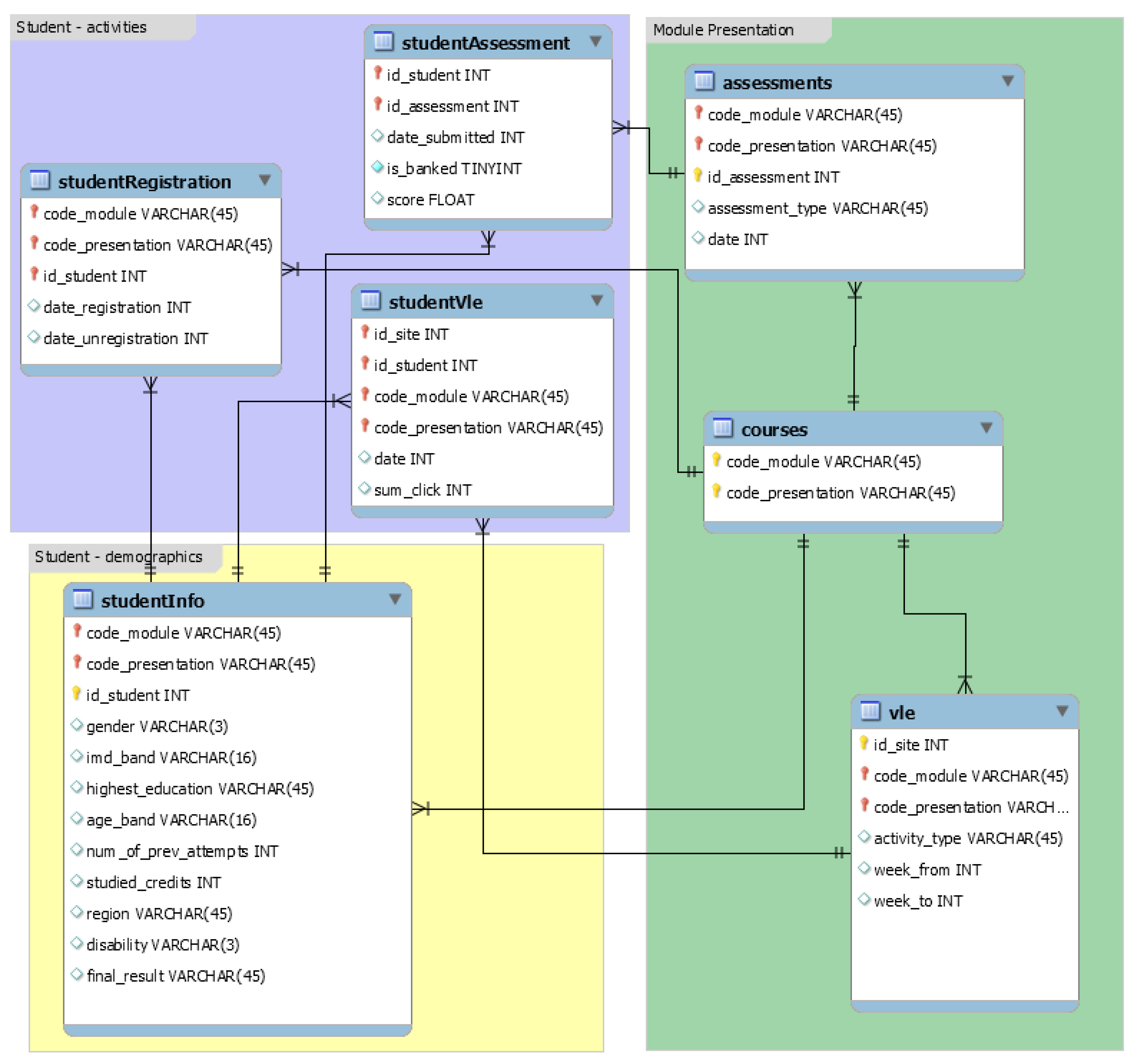
For our study, we used the Open University learning analytics dataset (OULAD) [77]. It consists of the information of 32,593 students studying 22 Open University courses during the years 2013 and 2014. The database schema of the OULAD dataset is shown in Figure 1.
Figure 1 shows that the OULAD database consists of seven different files. The course file contains information about the modules (courses) taught during the years 2013 and 2014. The assessments file contains the information related to the different assessments for each module. The VLE file contains information about the available materials in the VLE. Student demographic information is available in the studentInfo file. StudentRegistration includes information related to the date students registered and unregistered for the courses. The results of the assessment are stored in the studentAssessment file, and the studentVle file contains information related to the student’s involvement in the materials of the VLE. Each file mentioned needs to be processed to obtain the dataset ready for our study.
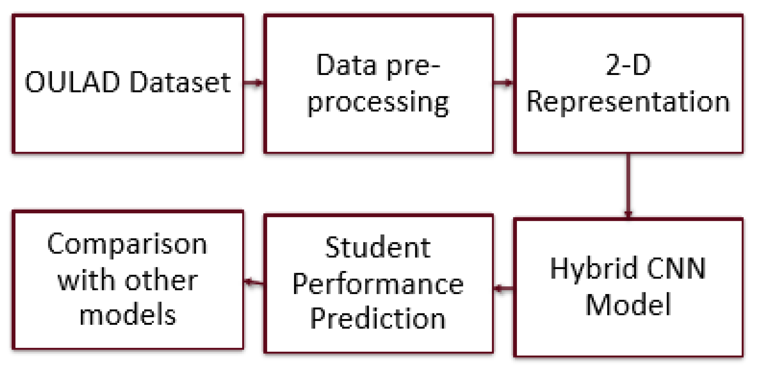
Figure 2 shows the proposed hybrid CNN model architecture.
Figure 2 shows our proposed model, which consists of six different stages. The first stage is the used dataset in our study, which we explained in Section 3. The second stage is the data preprocessing stage, which is explained in Section 3.1. The conversion of 1D data to a 2D image occurs in the third stage of our model, which is explained in Section 3.2. The fourth stage is our hybrid CNN model, which is explained in Section 3.3. The fifth stage is the student performance prediction stage, which is explained in Section 4, including an explanation of the performance prediction of our model in terms of pass and fail. In the last stage, we compared the performance of our model with some baseline models and with previous studies (Section 4.1).
3.1. Data Preprocessing
As explained before, there are seven different files that need to be processed. We used the Python platform to process all the files and obtain a single .csv file containing student demographic information, daily interaction with the university’s VLE, student assessment results, and final results of the students. The final results of the students were categorized as Distinction (n = 3024), Pass (n = 12,361), Fail (n = 7052), and Withdraw (n = 10,156). To make the binary classification, we combined Distinction and Pass as Pass (n = 15,385) and Fail and Withdraw as Fail (n = 17,208). Next, we had a categorical variable that needed to be changed to a numerical variable for our analysis. We performed one-hot encoding for our categorical variable to obtain the dataset with all the numerical variables.
3.2. 2D Representation
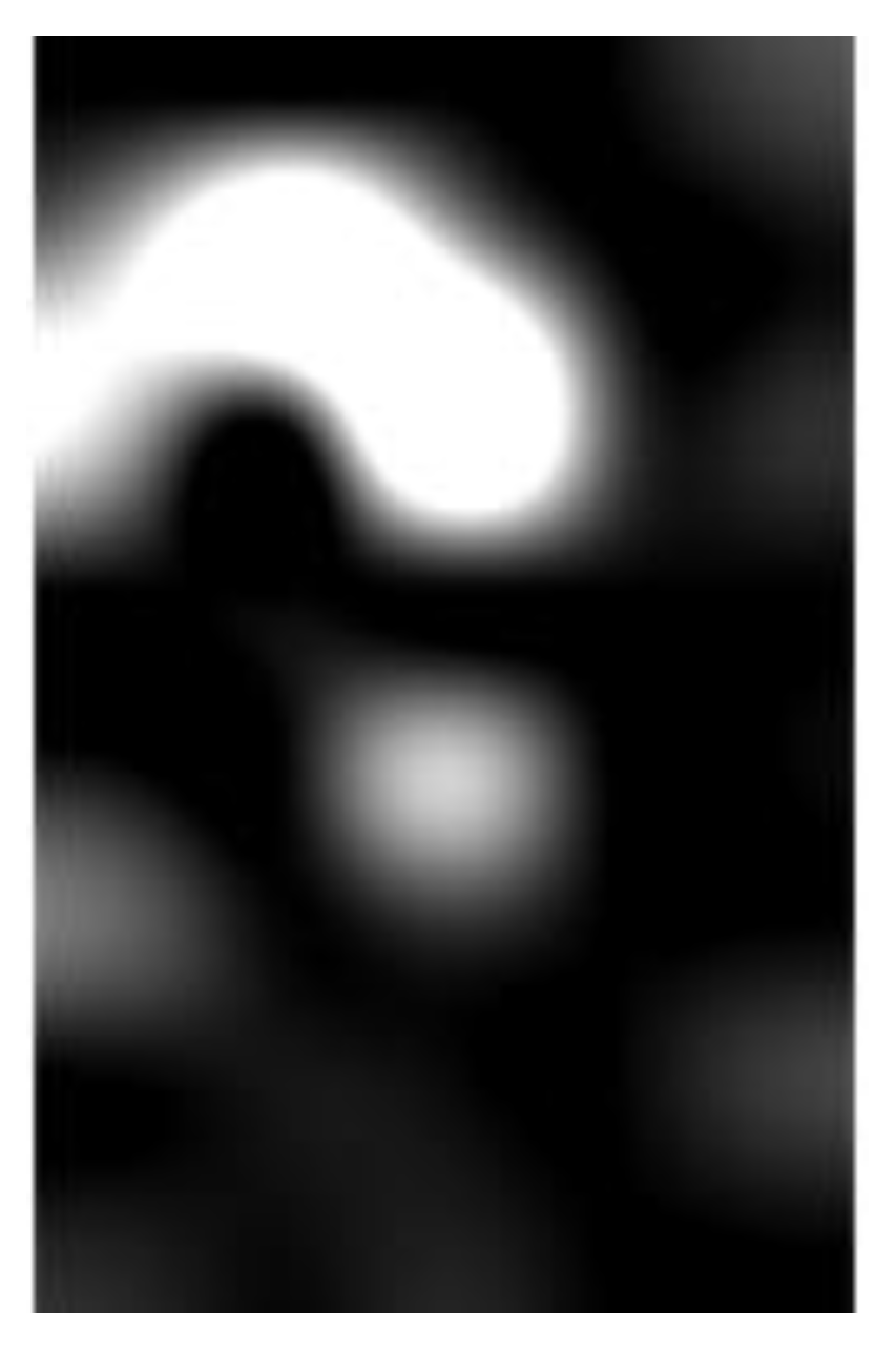
After the encoding, we obtained a dataset of 32,593 students. In our study, we used a 2D CNN, but our obtained data was 1D. Therefore, we transformed our data into a 2D format suitable for the 2D CNN architecture. After changing the categorical values to numerical values, we obtained a total of 37 numerical features. Each row now is the length of 37 sizes. To convert into 2D, we needed to perform zero padding to increase the features to 40 so that we could construct each 8 × 5 × 1 2D matrix. After zero padding, we performed reshaping so that each 40-length array was converted to an 8 × 5 × 1 size matrix. A 2D representation of each of the 32,593 students was obtained, for total of 32,593 images to be input into our 2D CNN architecture. Figure 3 shows the 2D representation of the sample input.
3.3. Approach
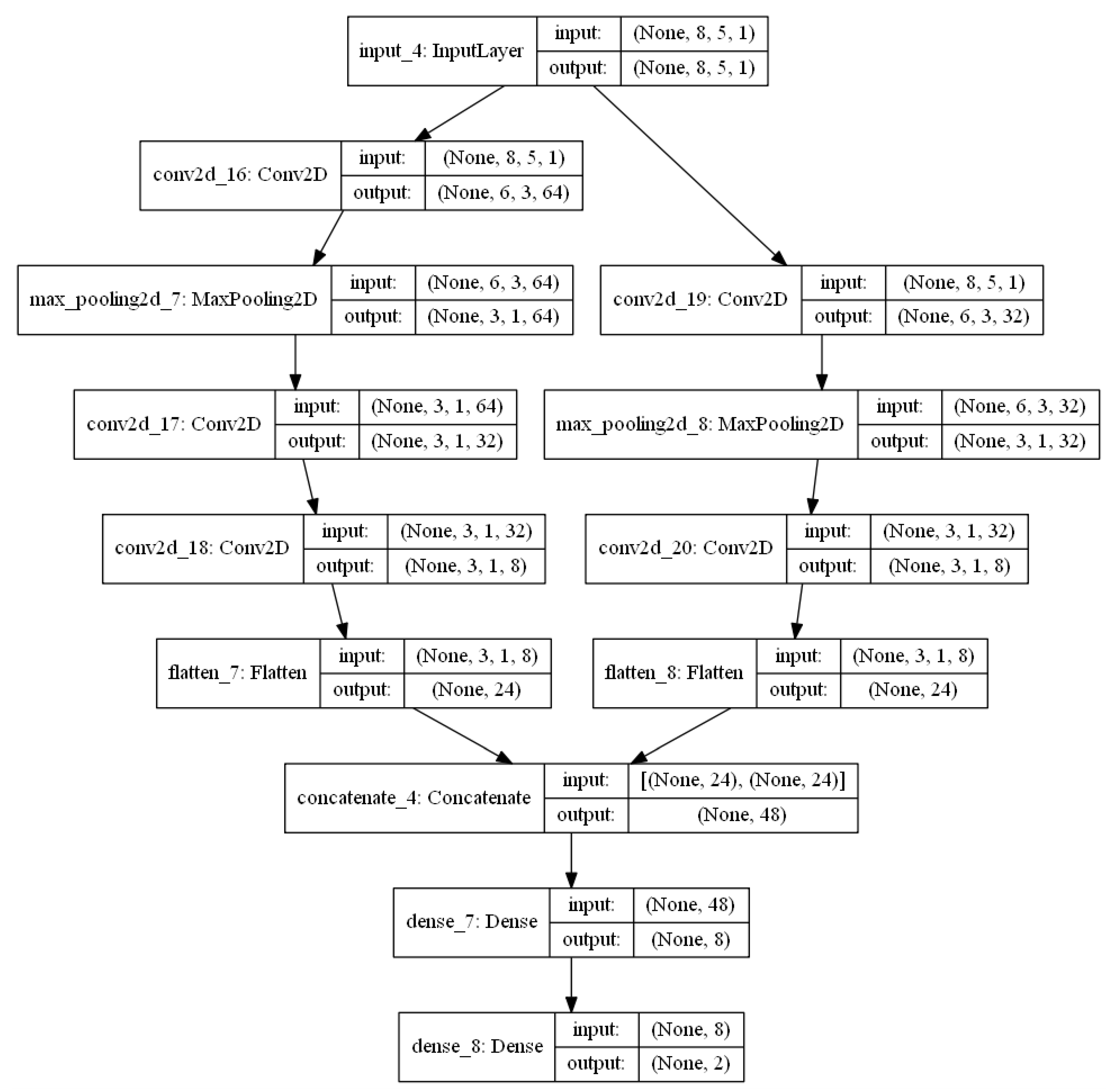
We applied a combination of two different 2D CNNs, each with a different number of layers. The model description of our study is shown in Figure 4.
From Figure 4, we can see that we have two different CNN models. As seen in Figure 4, the left model and the right model have six and five layers, respectively, before the dense layer.
Our model starts with the input layer, where the input is of size W × H × 1. The input is then passed to the first convolution layer of the first model. The convolution layer is used to detect the set of features from the input image. The filter is dragged onto the image, and convolution is performed between the filter and the input image to produce the feature map.
The convolutional layer has many hyperparameters. We defined how many filters we were using and the size of the filters. We defined the stride with which the filter was dragged across the image. The output of the convolutional layer is defined as obtained using Equations (1)–(3) [78].
where, S is a stride step (if S = 1, we move the filter one pixel at a time on the image); K is the number of filters used; F is the filter size; and W and H are the width and height of the input image, respectively.
From Figure 4, the input to the first convolutional layer is 8 × 5 × 1. The first convolutional layer has 64 filters, each of size 3 × 3, and the stride is one. Therefore, using Equations (1)–(3), the output will be 6 × 3 × 64 in size.
The third layer of the first model is the pooling layer. The pooling layer reduces the size of the images without losing much information. When reducing the size, it selects either the average value, referred to as average pooling, or the maximum value, referred to as max pooling. Pooling is usually performed with 2 × 2 patches with a stride of 2. The output of the pooling layer is defined as what is obtained using Equations (4)–(6).
where, S is stride step, F is filter size, and W and H are parameters of the input image.
In our study, we used max pooling. The input to our first pooling layer is 6 × 3 × 64. Using Equations (4)–(6), the output of the first pooling layer is 3 × 1 × 64, using a stride of 2.
The fourth layer of our first model is the convolution layer, and the input to it is an image of size 3 × 1 × 64. The second convolutional layer has 32 filters, each of size 1 × 1. Therefore, using Equations (1)–(3), the output is 3 × 1 × 32 in size. The fifth layer of our first model is again the convolutional layer with eight 1 × 1 filters. The obtained output of the convolutional layer using Equations (1)–(3) is 3 × 1 × 8 in size.
The pooled feature map is passed to the sixth layer, where flattening occurs to convert the input to the single layer 1D feature vector. The output of the flattened layer is supplied to the fully connected layer.
The input to our first flattening layer is 3 × 1 × 8, and its output is a long 1D vector with a length of 24.
In Figure 4, the input 8 × 5 × 1 image is applied to the second layer, which is the convolutional layer, with 32 3 × 3 filters and a stride step of 1. Using Equations (1)–(3), the output feature map of the second layer is 6 × 3 × 32 in size. The third layer is the max-pooling layer with a size of 2 × 2. Using Equations (4)–(6), the output of the third layer is 3 × 1 × 32. The fourth layer is a convolution layer, the output of which 3 × 1 × 8 in size, and the fifth layer is a flattening layer, which produces a long 1D vector with a length of 24.
Now, two models are concatenated, as shown in Figure 4. The output of this concatenating layer has a vector with a length of 48. The 48-length 1D vector is then passed to the fully connected layer. We used two dense layers for the fully connected layer. A dense layer is the layer of neurons where each neuron on the input is connected to each neuron on the output. The output of our first dense layer is a 1D vector with a size of 8. The last layer of our model is the dense layer, which has eight neurons on the input and two neurons on the output. This output is the final predicted output, which is compared with the original label to calculate the prediction accuracy.
We used an activation function in our model for the non-linearity transformation for the input signal. We used rectified linear units (ReLUs) for all the convolutional layers and the first dense layer in our model. Mathematically, ReLU is defined as y = max (0, x). It converts all the negative values to zero in the feature map. For the last dense layer, we used a sigmoid activation function to add non-linearity to the input signal.
The learning algorithm for our hybrid 2D CNN can be summarized as follows:
- Take the input data and reshape each datum to 2D to obtain each input datum of size W × H × D.
- For the first convolutional layer, define the total number of filters, K; filter size, F; and stride step, S, and calculate the output feature map with a size of , where:
- The feature map, , is an input to the first pooling layer. For the first pooling layer, define filter size, F, and stride step, S, and calculate the output of the size of , where:
- For the second convolutional layer, define the total number of filters, K; filter size, F; and stride step, S, and calculate the output feature map with a size of , where:
- For the third convolutional layer, define the total number of filters, K; filter size, F; and stride step, S, and calculate the output feature map with a size of , where:
- The output of step 5 is converted to the single-layer 1D vector in the first flattened layer.
- For the fourth convolutional layer, the input is the original input with a size of W × H × D. Calculate the output feature map with a size of , where:
- For the second pooling layer, define the filter size, F, and stride step S, and calculate the output with a size of , where:
- For the fifth convolutional layer, define the total number of filters, K; filter size, F; and stride step, S, and calculate the output feature map with a size of , where:
- The output of step 9 is converted to the single-layer 1D vector in the second flattened layer.
- Concatenate the output obtained from steps 6 and 9 to produce a 1D long vector, which becomes the input to the fully connected layer.
- Define the number of input neurons and output neurons for the first dense layer. Pass the output to the second dense layer.
- For the second dense layer, define the output neurons as the total number of classes in our dataset.
- Predict the label and calculate the accuracy.
4. Experimentation and Evaluation
We split our dataset, with 70% as a training test and the remaining 30% as a test set. We also used the test data as the validation data. Therefore, in this study, test loss and test accuracy mean validation loss and accuracy, respectively. We used accuracy as our performance metric. We performed parameter tuning to obtain the best results.
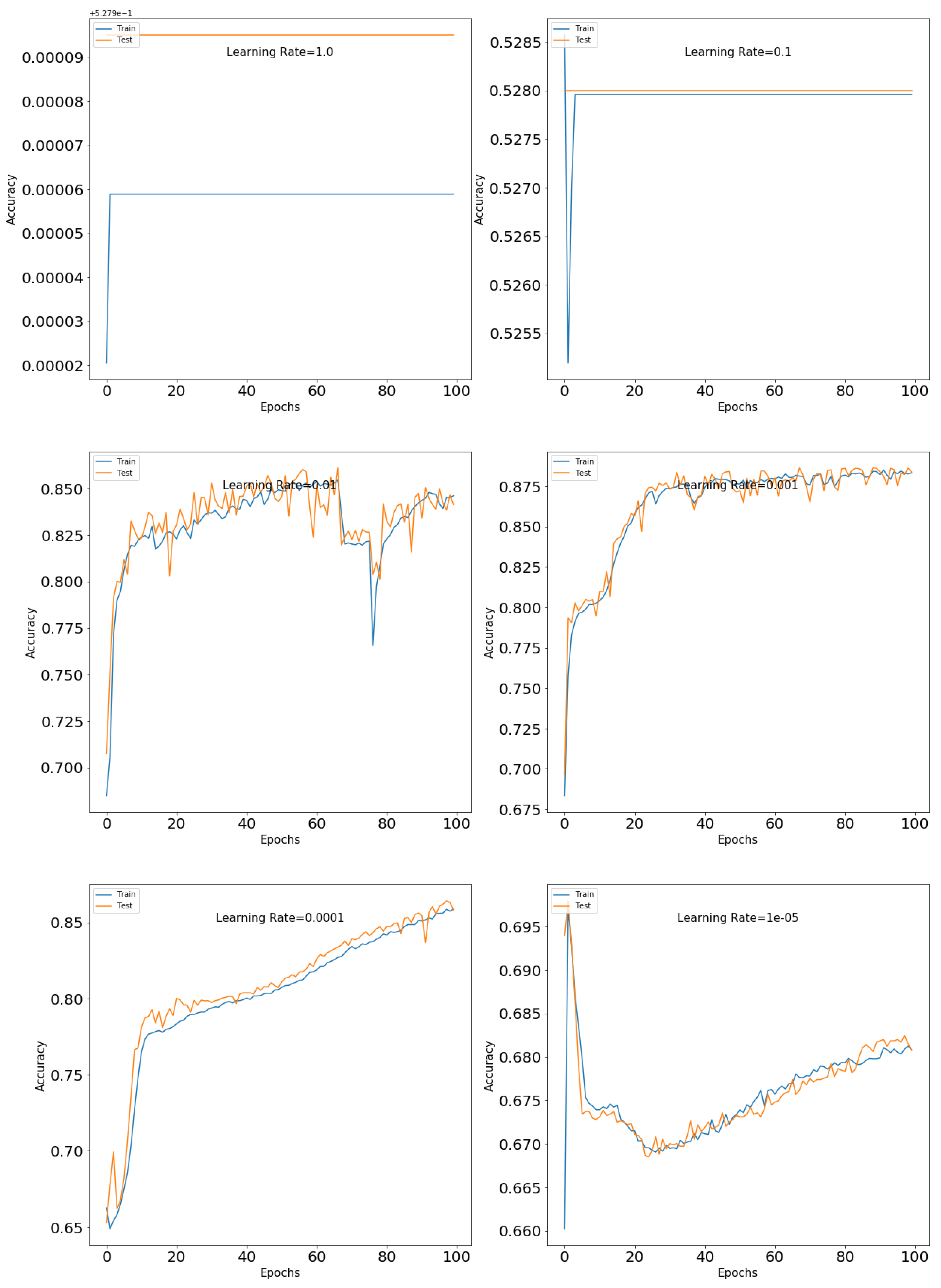
Learning rate is an important parameter. Therefore, we used different learning rates to see which one performed the best for our model. Learning rate is a small positive value, often in the range of 0–1, and is used to train data. The learning rate is used to control how fast the model adapts to the problem. A learning rate that is too high can lead the model to converge too rapidly to a poor solution, whereas a learning rate that is too low can cause the process to get stuck. Therefore, we must select the perfect learning rate. We ran our model with different learning rates, and the result is shown in Table 1. We also plotted the training and test accuracy for different learning rates, which is shown in Figure 5.
Table 1 shows the test loss and test accuracy for different learning rates. We obtained the highest accuracy with a learning rate of 0.001. As we can see in Figure 5, the learning curve is flat for higher learning rates (for 1 and 0.1). This is because the model was not able to learn anything at a higher learning rate. The plot shows oscillating behavior for the lower learning rates. For our model, the result shows that a learning rate of 0.001 is optimal, as it produces good model performance, as seen in Figure 5.
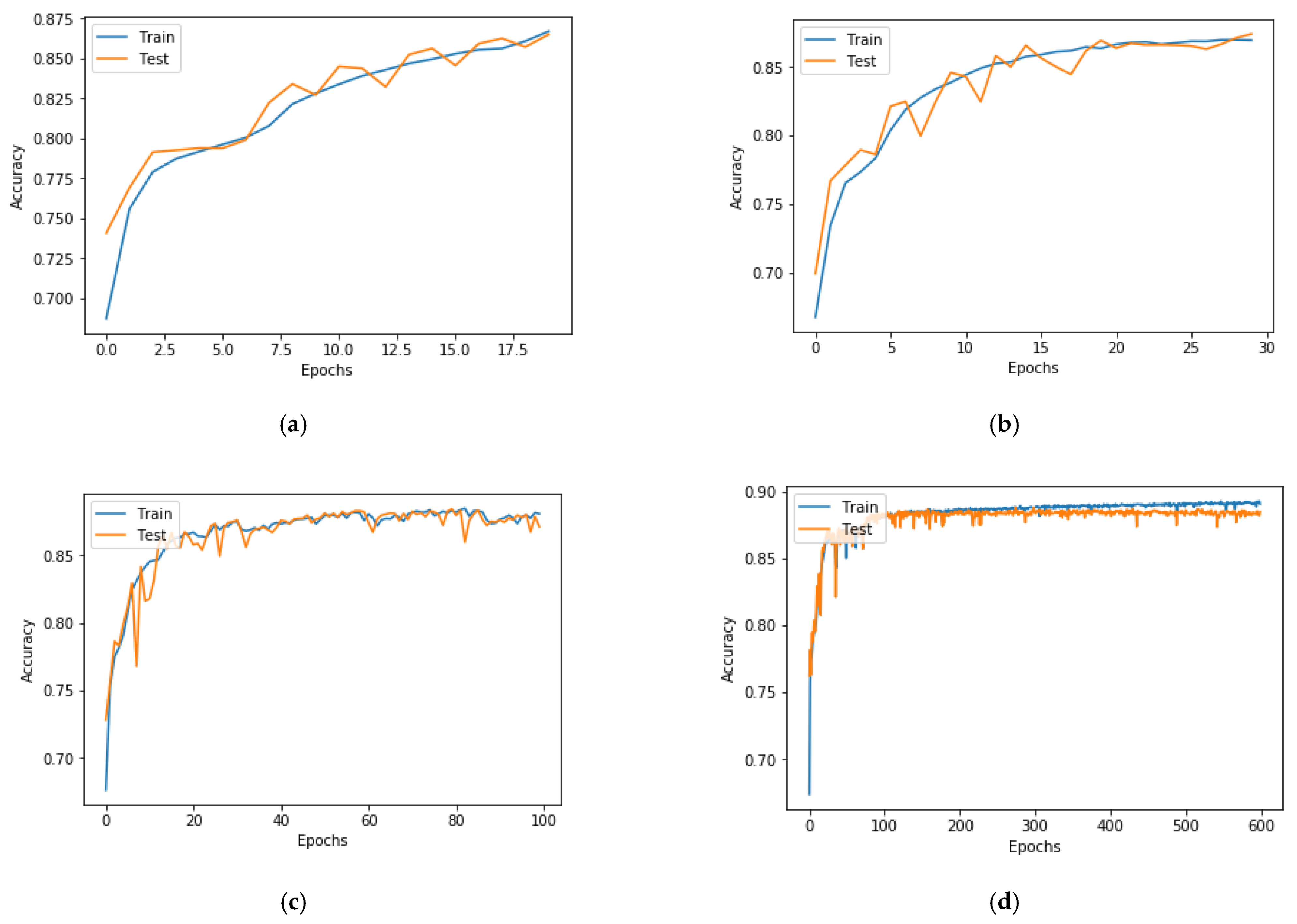
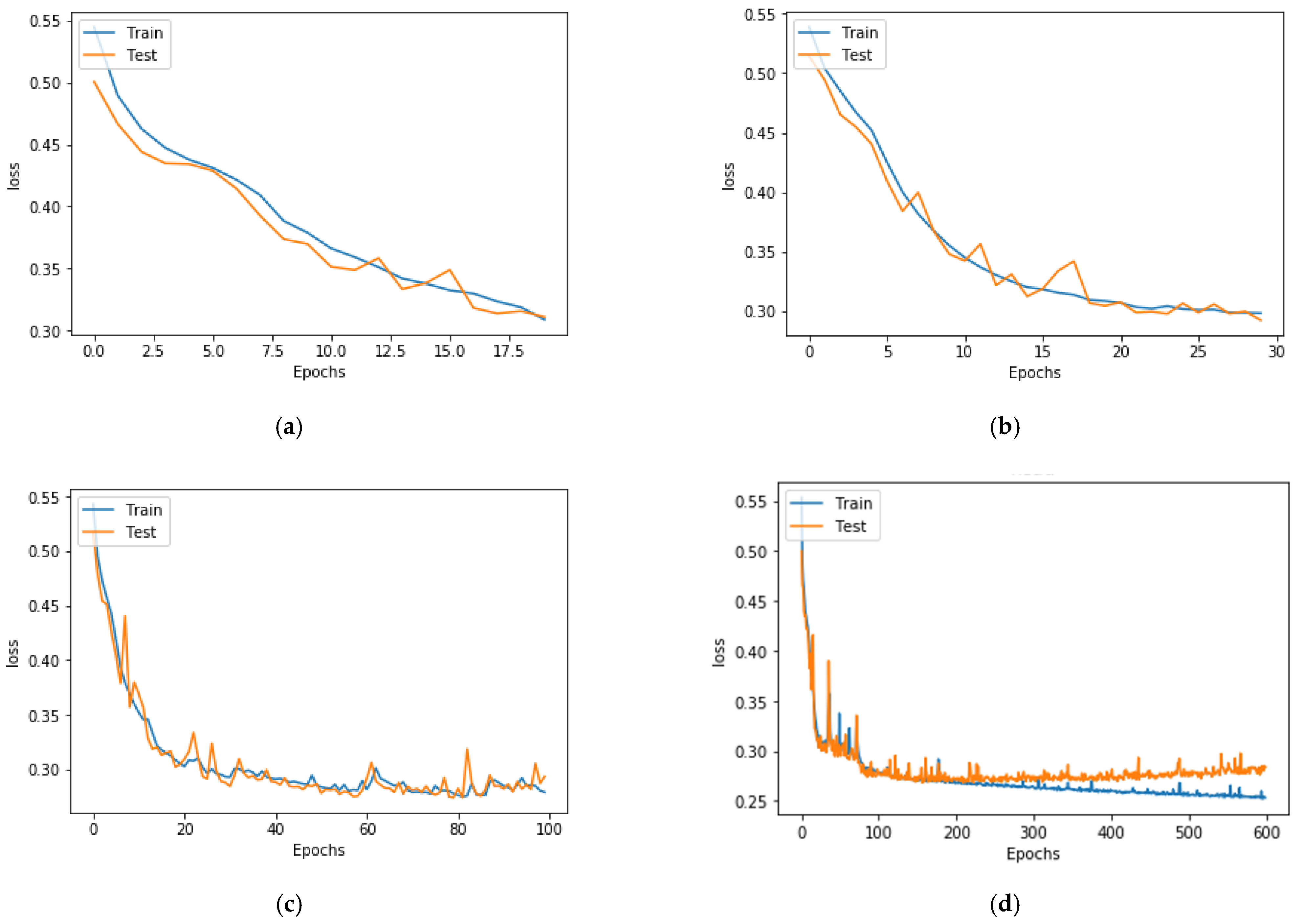
We used different numbers of epochs to determine the accuracy of the model and observed the plots of accuracy vs. epochs and loss vs. epochs. We increased the number of epochs from 20 to determine its effect on model performance. Test loss and test accuracy are shown in Table 2, and the accuracy and loss plots are shown in Figure 6 and Figure 7, respectively.
Table 2 shows the test loss and test accuracy for different numbers of epochs. We obtained the highest accuracy of 0.88 with 100 epochs. We started with 20 epochs, with which we obtained an accuracy of 0.86. We then increased the number of epochs to 30 and obtained an accuracy of 0.87. Using 20 and 30 epochs, the accuracy and loss plot in Figure 6 and Figure 7, respectively, show that the model was learning. We continued to increase the number of epochs up to 100, at which point saw observed changes in the loss plot, as shown in Figure 7c. As we further increased the number of epochs to 600, test loss increased, as seen in Figure 7d. This is due e overfitting. Therefore, to determine the optimal number of epochs, we used the early stopping criteria. When both the training and test loss in the plot decreased as we increased the number of epochs, it was a good sign that the model is learning well; however, as the test loss began to increase, we stopped the training process. This is called early stopping. Using this process, we obtained determined the optimal epoch to be 100 for our model.
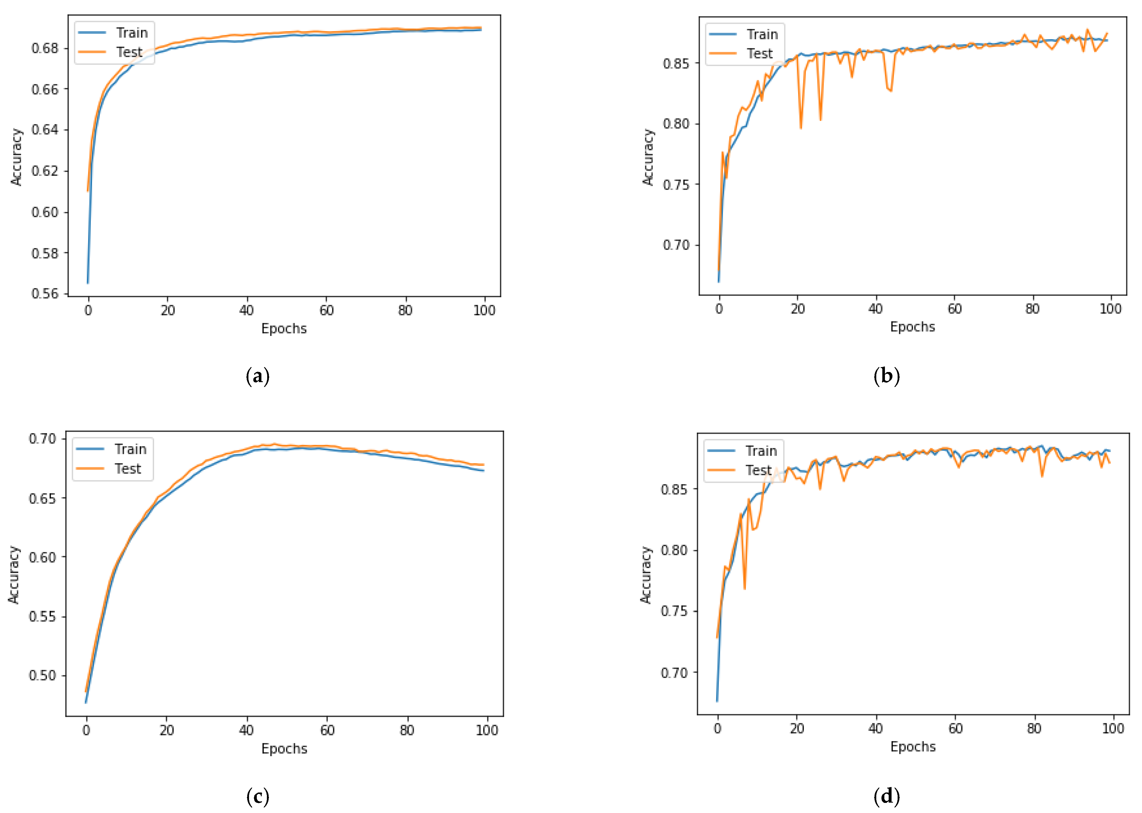
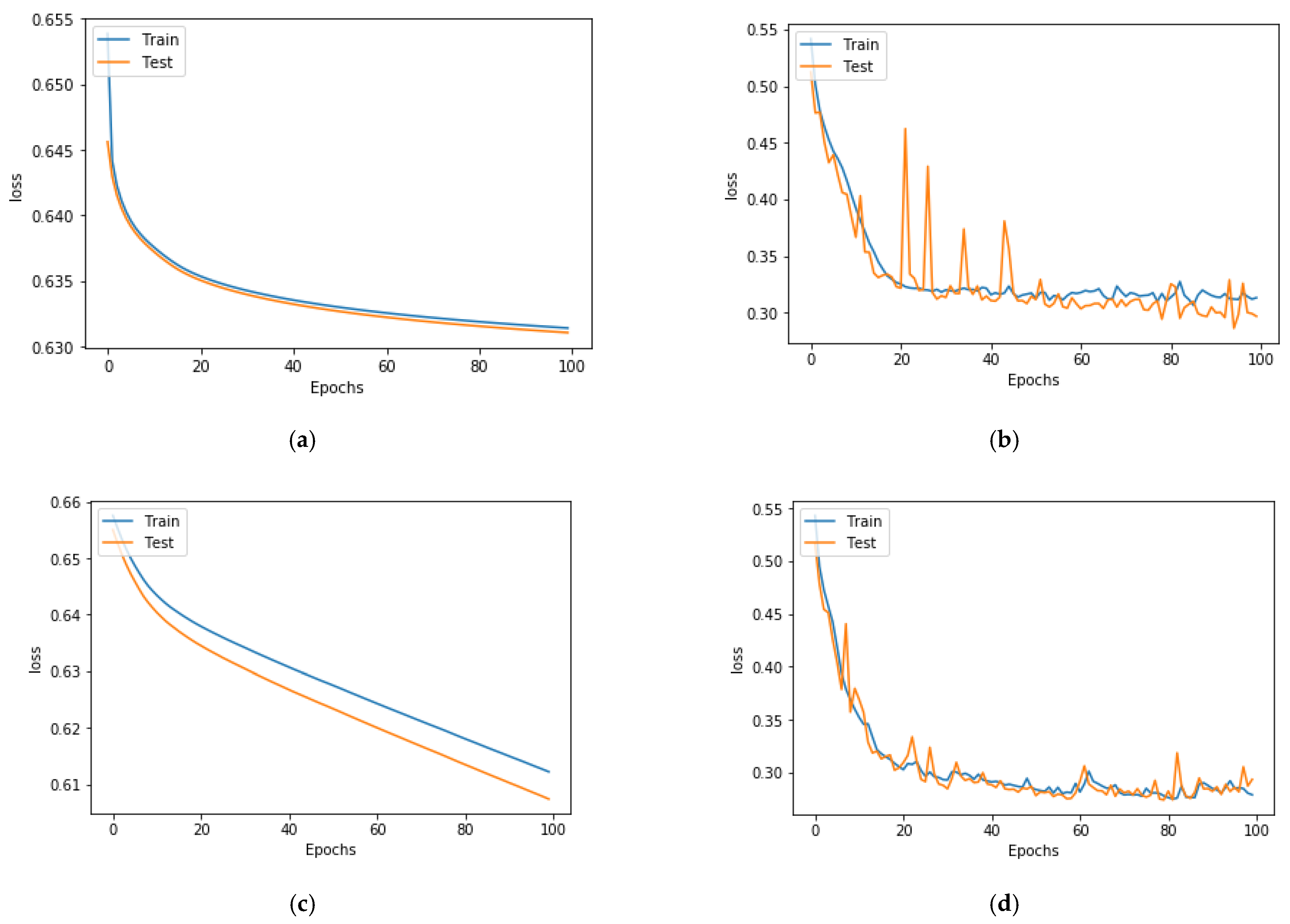
We also used different optimizers to observe the effects on test accuracy and test loss. We used stochastic gradient descent (SGD), Adadelta, root mean square propagation (RMSprop), and adaptive moment (Adam) as the optimizers. Accuracy is shown in Table 3, and the accuracy and loss plots are shown in Figure 8 and Figure 9, respectively. We used a learning rate of 0.001 with 100 for all the experiments to determine the effect of different optimizers on test loss and test accuracy.
Table 3 shows the test accuracy and test loss for using different optimizers. When we used the RMSprop optimizer, although the test accuracy was high at 0.87, we can see that there is high oscillation on the accuracy and loss plots, as seen in Figure 8b and Figure 9b, respectively. For the Adadelta and SGD optimizers, the loss plot, as seen in Figure 9, shows that the training loss and the test loss both decrease continuously at the end of the plot. This is due to the underfitting. Therefore, the test accuracy is only 0.68 and 0.69 when using the Adadelta and SGD optimizers, respectively. When using the Adam optimizer, the accuracy plot goes on, increasing to the point of stability, as seen in Figure 8d. Additionally, as seen in the loss plot, training loss continues to decrease up to the point of stability, whereas test loss also decreases and maintains a small gap with the training loss. The learning curve for the Adam optimizer, as shown in Figure 8d, is a decent match, and the model learns effectively with a test accuracy of 0.88.
4.1. Evaluation with Baseline Model and Previous Studies
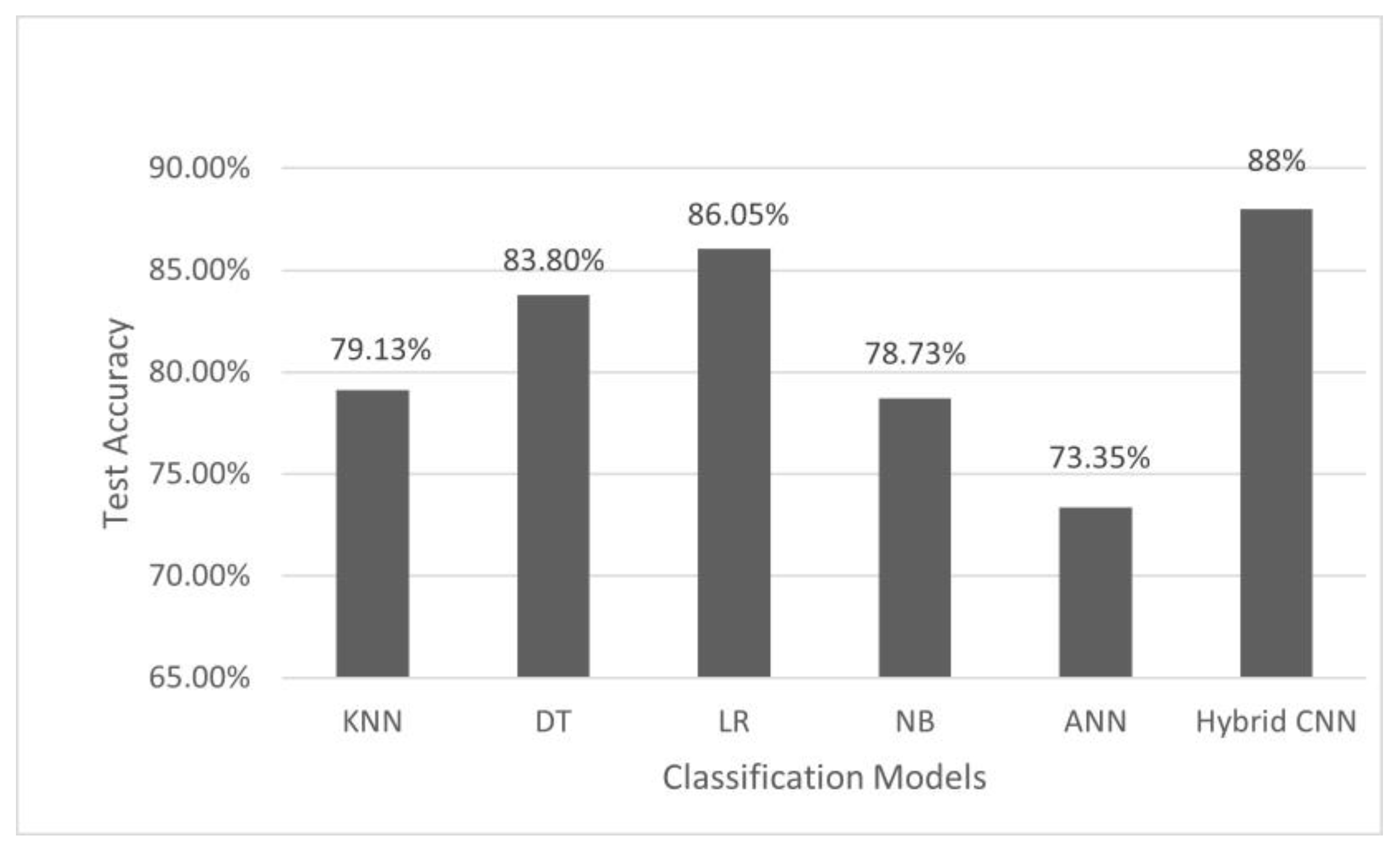
We used different baseline models to run on our data to predict the academic performance of students. In educational data mining research, models such as KNN, DT, LR, NB, and ANN are frequently adopted to predict student academic performance. We also used these models as our baseline models to compare performance with that of our hybrid CNN model. The performance comparison of our hybrid CNN model was performed with these baseline traditional models based on test accuracy. The result is shown in Figure 10.
Figure 10 shows that ANN performed the worst, with a very low test accuracy of only 73.75%. Among the baseline models, LR performed well, with an accuracy of 86.05%. Our hybrid CNN model achieved the best results among all models, with a test accuracy of 88%.
We also compared the performance of our models with that of models reported in previous studies. Table 4 shows the comparison of our model with different previously reported models.
5. Implications of Results
Extensive research has been done on educational data mining to predict student academic performance. Many methods, ranging from traditional methods to deep learning methods, have been applied to educational data mining. We used deep learning methods in our study. We used the OULAD dataset and preprocessed the data as described in Section 3.1 to obtain the problem binary classifications. As explained in Section 1, one of the objectives of this study was to convert 1D numerical data to 2D image data. We fulfilled this objective by reshaping our data with 40 features to obtain an 8 × 5 grayscale image, which is explained in detail in Section 3.2. Our second objective was to build a hybrid CNN model. We combined two CNNs with different convolutional and pooling sizes and obtained a single hybrid CNN model, as explained in Section 3.3.
Our final objective was to test the performance of the proposed hybrid model and compare it with that of baseline models. We used different learning rates to determine the performance of our model. We achieved the highest accuracy with a learning rate of 0.001. The learning curve at higher learning rates is flat, as seen in Figure 5 (for 1 and 0.1). The reason for this is that the model was unable to learn anything at a faster rate. The graph in Figure 5 demonstrates oscillatory behavior with a reduced learning rate. As shown in Figure 5, a learning rate of 0.001 is ideal for our model because it achieves high model performance. To test the performance of our hybrid model, we employed several numbers of epoch, and the best results were obtained with test loss of 0.28 and a test accuracy of 0.88 for 100 epochs, as shown in Table 2. As we further increased the number of epochs to 600, test loss increased, as seen in Figure 7d, which is due to overfitting. We used the early stopping criteria and obtained the 100 as the optimal number of epochs for our model. We used different optimizers to determine the performance of our hybrid model and obtained the best results with a test loss of 0.28 and a test accuracy of 0.88 with Adam optimizers, as shown in Table 3. When using other optimizers besides Adam, our results did not improve, which can be seen in Figure 8 and Figure 9. For comparison, we used different baseline models, such as KNN, DT, LR, NB, and ANN. As shown in Figure 10, our hybrid model outperformed the baseline traditional models in terms of accuracy.
We compared the performance of our model with that reported in previous studies, as shown in Table 4. Reference [54] used techniques such as DT, RF, extreme gradient boosting, and MLP to predict the academic performance of students. MLP performed the best, with the highest accuracy of 78.2%. Reference [55] used NB, KNN, LDA, SVM, and MLP and obtained the highest accuracy of 76.3% with SVM. Reference [76] used CNN and LSTM and obtained an accuracy of 61% for predicting academic performance. Reference [50] used DT and obtained an accuracy of 83.14%. Reference [56] used NB and DT, and NB obtained the highest accuracy of 63.8%. All of these studies used the OULAD dataset, except [55], which used a private dataset of student dissertation project grades. Our hybrid model obtained an accuracy of 88% and outperformed all the models reported in these studies. Our hybrid model outperformed the baseline model and the models of previous studies. Therefore, in response to our research question, our hybrid CNN can be applied to numerical 1D educational datasets to predict students academic performance.
Our study is subject to some limitations. First, because we had only 37 features in our study, the obtained image after 1D-to-2D transformation was of a small size, i.e., 8 × 5. Because of this, we could not use more pooling layers in our model. Therefore, for each model, we could only use one pooling layer. The second limitation of our study is that we exclusively used accuracy as a criterion for measuring performance. Third, we predicted the academic performance of students but did not study the impact of each feature on academic performance.
6. Conclusions
A multitude of data is being produced by institutional technology, e-learning resources, and online and virtual courses. These data could be used by educators to analyze and understand the learning behaviors of students. The data that is obtained from the pedagogical domain is in raw form, and we need EDM to extract information from such raw data. When educational raw data is observed, it helps to know who failed or passed, but the EDM extracts hidden information from such raw data and helps to analyze and predict, with high accuracy, whether the students are going to pass or fail. To test such a prediction, we built a hybrid 2D CNN architecture that can predict whether students will pass or fail a class. Our data were 1D data, which we converted to 2D data so that we could apply 2D CNN to our dataset. As shown in Section 4, we were able to predict academic performance with high accuracy. A high accuracy of 88% was achieved by our model. This positively supports our research question. We also performed parameter tuning to obtain the best results. For parameter tuning, we used different learning rates, numbers of epochs, and optimizers. The result is seen in Table 1, Table 2 and Table 3. The plots with different epochs numbers in Figure 6 and Figure 7 help to visually display that performance is best at 100 epochs. Additionally, among the investigated optimizers, Adam performed the best, which can be seen visually from the plots in Figure 8 and Figure 9. As seen in Figure 10, our model outperformed the baseline traditional models in terms of accuracy. Our hybrid model obtained an accuracy of 88% and outperformed all models reported in previous studies, as shown in Table 4. Therefore, in response to our research question, our hybrid CNN can be applied to numerical 1D educational datasets to predict student academic performance.
We were able to work with a numerical 1D dataset by reshaping all of the data into a 2D image. As a result, the 2D data had a modest matrix size. We may be able to employ large image data from the pedagogical sector in the future to better grasp the depth of deep learning capability in EDM. We used accuracy alone as a performance metric. In the future, we can see how our model affects other performance metrics, kappa, recall, and sensitivity. We did not investigate the impact of each feature on academic performance in this study; this is something we plan to tackle in the future. Because our dataset is small, explainable AI is an interesting topic that could be included in the future. Explainable AI is ideal for smaller datasets. The current study demonstrates how educational institutions could use CNN architecture to anticipate student academic performance and take appropriate action to assist students. Our model’s great accuracy has prompted us to continue experimenting with CNN architecture in the pedagogical sector.
Author Contributions
Conceptualization, S.P and M.J.M.-A.; methodology, S.P. and J.E.B.; software, S.P.; validation, S.P.; formal analysis, S.P.; investigation, S.P.; resources, S.P.; data curation, S.P.; writing—original draft preparation, S.P. and M.J.M.-A.; writing—review and editing, S.P., M.J.M.-A. and J.E.B.; visualization, S.P.; supervision, M.J.M.-A.; project administration, M.J.M.-A.; funding acquisition, M.J.M.-A. All authors have read and agreed to the published version of the manuscript.
Funding
This material is based upon work supported in part by the National Science Foundation under grant 2047625.
Institutional Review Board Statement
Not applicable.
Data Availability Statement
Publicly available datasets were analyzed in this study. This data can be found here: https://analyse.kmi.open.ac.uk/open_dataset (accessed on 25 September 2021).
Acknowledgments
We appreciate the anonymous reviewers’ time and effort in reading our paper despite their busy schedules, as well as their many insightful comments and ideas.
Conflicts of Interest
The authors declare no conflict of interest.
References
- Here’s How Much Your High School Grades Predict Your Future Salary. Available online: https://www.washingtonpost.com/news/wonk/wp/2014/05/20/heres-how-much-your-high-school-grades-predict-how-much-you-make-today/ (accessed on 2 November 2021).
- Koh, H.; Tan, G. Data mining applications in healthcare. J. Healthc. Inf. Manag. 2005, 19, 64–72. [Google Scholar] [PubMed]
- Sodhro, A.H.; Zahid, N. AI-Enabled Framework for Fog Computing Driven E-Healthcare Applications. Sensors 2021, 21, 8039. [Google Scholar] [CrossRef] [PubMed]
- Vazan, P.; Janikova, D.; Tanuska, P.; Kebisek, M.; Cervenanska, Z. Using data mining methods for manufacturing process control. IFAC-Pap. 2017, 50, 6178–6183. [Google Scholar] [CrossRef]
- Awoyemi, J.O.; Adetunmbi, A.O.; Oluwadare, S.A. Credit card fraud detection using machine learning techniques: A comparative analysis. In Proceedings of the International Conference on Computing Networking and Informatics (ICCNI), Lagos, Nigeria, 29–31 October 2017. [Google Scholar]
- Lan, K.; Wang, D.; Fong, S. A Survey of Data Mining and Deep Learning in Bioinformatics. J. Med. Syst. 2018, 42, 139. [Google Scholar] [CrossRef] [PubMed]
- Farzaneh, A.; Fadlalla, A. Data mining applications in accounting: A review of the literature and organizing framework. Int. J. Account. Inf. Syst. 2017, 24, 32–58. [Google Scholar]
- Ghosh, I.; Datta Chaudhuri, T. FEB-Stacking and FEB-DNN Models for Stock Trend Prediction: A Performance Analysis for Pre and Post COVID-19 Periods. Decis. Mak. Appl. Manag. Eng. 2021, 4, 51–84. [Google Scholar] [CrossRef]
- Shah, C.; Du, Q.; Xu, Y. Enhanced TabNet: Attentive Interpretable Tabular Learning for Hyperspectral Image Classification. Remote Sens. 2022, 14, 716. [Google Scholar] [CrossRef]
- More Students are Learning on Laptops and Tablets in Class. Some Parents Want to Hit the Off Switch. Available online: https://www.washingtonpost.com/local/education/more-students-are-learning-on-laptops-and-tablets-in-class-some-parents-want-to-hit-the-off-switch/2020/02/01/d53134d0-db1e-11e9-a688-303693fb4b0b_story.html (accessed on 1 November 2021).
- Get the 411: Laptops and Tablets in the Classroom. Available online: https://www.educationworld.com/a_tech/tech/tech194.shtml (accessed on 25 September 2021).
- How to Implement 1:1 Technology using Tablets in the Classroom. Available online: https://myelearningworld.com/10-benefits-of-tablets-in-the-classroom/ (accessed on 28 September 2021).
- Virtual Reality in Education: Benefits, Tools, and Resources. Available online: https://soeonline.american.edu/blog/benefits-of-virtual-reality-in-education (accessed on 25 September 2021).
- Hasan, R.; Palaniappan, S.; Mahmood, S.; Abbas, A.; Sarker, K.U.; Sattar, M.U. Predicting Student Performance in Higher Educational Institutions Using Video Learning Analytics and Data Mining Techniques. Appl. Sci. 2020, 10, 3894. [Google Scholar] [CrossRef]
- Nagahi, M.; Jaradat, R.; Nagahisarchoghaei, M.; Ghanbari, G.; Poudyal, S.; Goerger, S. Effect of Individual Differences in Predicting Engineering Students’ Performance: A Case of Education for Sustainable Development. In Proceedings of the International Conference on Decision Aid Sciences and Applications (DASA), Online, 8–9 November 2020. [Google Scholar]
- Okubo, F.; Yamashita, T.; Shimada, A.; Ogata, H. A neural network approach for students’ performance prediction. In Proceedings of the Seventh International Learning Analytics & Knowledge Conference (LAK ‘17), Vancouver, BC, Canada, 13–17 March 2017; Association for Computing Machinery: New York, NY, USA, 2017. [Google Scholar]
- Byung-Hak, K.; Ethan, V.; Ganapathi, V. GritNet: Student Performance Prediction with Deep Learning. arXiv 2018, arXiv:1804.07405. [Google Scholar]
- Wang, W.; Yu, H.; Miao, C. Deep Model for Dropout Prediction in MOOCs. In Proceedings of the 2nd International Conference on Crowd Science and Engineering (ICCSE’17), Beijing, China, 6–9 July 2017. [Google Scholar]
- Whitehill, J.; Mohan, K.; Seaton, D.; Rosen, Y.; Tingley, D. Delving Deeper into MOOC Student Dropout Prediction. arXiv 2017, arXiv:1702.06404. [Google Scholar]
- Xing, W.; Dongping, D. Dropout Prediction in MOOCs: Using Deep Learning for Personalized Intervention. J. Educ. Comput. Res. 2019, 57, 547–570. [Google Scholar] [CrossRef]
- Bohong, Y.; Zeping, Y.; Hong, L.; Yaqian, Z.; Jinkai, X. In-classroom learning analytics based on student behavior, topic and teaching characteristic mining. Pattern Recognit. Lett. 2020, 129, 224–231. [Google Scholar]
- Nigel, B.K.; D’mello, S.; Ocumpaugh, J.; Baker, R.; Shute, V. Using Video to Automatically Detect Learner Affect in Computer-Enabled Classrooms. ACM Trans. Interact. Intell. Syst. 2016, 6, 1–26. [Google Scholar]
- Goldberg, P.; Sümer, O.; Stürmer, K. Attentive or Not? Toward a Machine Learning Approach to Assessing Students’ Visible Engagement in Classroom Instruction. Educ. Psychol. 2021, 33, 27–49. [Google Scholar] [CrossRef] [Green Version]
- Cetintas, S.; Si, L.; Xin, P.; Hord, C. Automatic Detection of Off-Task Behaviors in Intelligent Tutoring Systems with Machine Learning Techniques. IEEE Trans. Learn. Technol. 2010, 3, 228–236. [Google Scholar] [CrossRef]
- Zaletelj, J.; Košir, A. Predicting students’ attention in the classroom from Kinect facial and body features. J. Image Video Proc. 2017, 80, 80. [Google Scholar] [CrossRef]
- Antoniou, P.E.; Arfaras, G.; Pandria, N.; Athanasiou, A.; Ntakakis, G.; Babatsikos, E.; Bamidis, P. Biosensor real-time affective analytics in virtual and mixed reality medical education serious games: Cohort study. JMIR Serious Games 2020, 8, e17823. [Google Scholar] [CrossRef] [PubMed]
- Ahonen, L.; Cowley, B.U.; Hellas, A.; Puolamaki, K. Biosignals reflect pair-dynamics in collaborative work: EDA and ECG study of pair-programming in a classroom environment. Sci. Rep. 2018, 8, 3138. [Google Scholar] [CrossRef] [PubMed]
- Magsi, H.; Sodhro, A.H.; Al-Rakhami, M.S.; Zahid, N.; Pirbhulal, S.; Wang, L. A Novel Adaptive Battery-Aware Algorithm for Data Transmission in IoT-Based Healthcare Applications. Electronics 2021, 10, 367. [Google Scholar] [CrossRef]
- Sumyea, H.; Jiuyong, L.; Lin, L.; Esmaeil, E.; Shane, D.; Duncan, M.; Qi, L. Predicting academic performance by considering student heterogeneity. Knowl. Based Syst. 2018, 161, 134–146. [Google Scholar]
- Hussain, S.; Abdulaziz Dahan, N.; Ba-Alwib, F.; Najoua, R. Educational Data Mining and Analysis of Students’ Academic Performance Using WEKA. Indones. J. Electr. Eng. Comput. Sci. 2018, 9, 447–459. [Google Scholar] [CrossRef]
- Sharma, A.; Vans, E.; Shigemizu, D. DeepInsight: A methodology to transform a non-image data to an image for convolution neural network architecture. Sci. Rep. 2019, 9, 11399. [Google Scholar] [CrossRef] [PubMed] [Green Version]
- Loka, N.R.B.S.; Kavitha, M.; Kurita, T. Hilbert Vector Convolutional Neural Network: 2D Neural Network on 1D Data. In Proceedings of the International Conference on Artificial Neural Networks (ICANN), Munich, Germany, 17–19 September 2019. [Google Scholar]
- Al-Turaiki, I.; Altwaijry, N. A Convolutional Neural Network for Improved Anomaly-Based Network Intrusion Detection. Big Data 2021, 9, 233–252. [Google Scholar] [CrossRef]
- Nagahisarchoghaei, M.; Dodd, J.; Nagahi, M.; Ghanbari, G.; Poudyal, S. Analysis of a Warranty-Based Quality Management System in the Construction Industry. In Proceedings of the International Conference on Data Analytics for Business and Industry: Way Towards a Sustainable Economy (ICDABI), Online, 26–27 October 2020. [Google Scholar] [CrossRef]
- Shah, C.; Du, Q. Modified Structure-Aware Collaborative Representation for Hyperspectral Image Classification. In Proceedings of the 2021 IEEE International Geoscience and Remote Sensing Symposium IGARSS, Brussels, Belgium, 11–16 July 2021. [Google Scholar]
- Shah, C.; Du, Q. Spatial-Aware Collaboration-Competition Preserving Graph Embedding for hyperspectral image classification. IEEE Geosci. Remote Sens. Lett. 2021, 19, 1–5. [Google Scholar] [CrossRef]
- Shah, C.; Du, Q. Collaborative and Low-Rank Graph for Discriminant Analysis of Hyperspectral Imagery. IEEE J. Sel. Top. Appl. Earth Obs. Remote. Sens. 2021, 14, 5248–5259. [Google Scholar] [CrossRef]
- Aulck, L.; Velagapudi, N.; Blumenstock, J.; West, J. Predicting student dropout in higher education. In Proceedings of the ICML Workshop on #Data4Good: Machine Learning in Social Good Applications, New York, NY, USA, 24 June 2016; Available online: https://arxiv.org/pdf/1606.06364.pdf (accessed on 28 September 2021).
- Daud, A.; Aljohani, N.R.; Abbasi, R.A.; Lytras, M.D.; Abbas, F.; Alowibdi, J.S. Predicting student performance using advanced learning analytics. In Proceedings of the 26th International Conference on World Wide Web Companion, Perth, Australia, 3–7 April 2017. [Google Scholar] [CrossRef] [Green Version]
- Garg, R. Predicting student performance of different regions of Punjab using classification techniques. Int. J. Adv. Res. Comput. Sci. 2018, 9, 236–241. [Google Scholar] [CrossRef] [Green Version]
- Kemper, L.; Vorhoff, G.; Wigger, B.U. Predicting student dropout: A machine learning approach. Eur. J. High. Educ. 2020, 10, 28–47. [Google Scholar] [CrossRef]
- Aluko, R.O.; Daniel, E.I.; Oshodi, O.S.; Aigbavboa, C.O.; Abisuga, A.O. Towards reliable prediction of academic performance of architecture students using data mining techniques. J. Eng. Des. Technol. 2018, 16, 385–397. [Google Scholar] [CrossRef] [Green Version]
- Luhaybi, M.A.; Tucker, A.; Yousefi, L. The prediction of student failure using classification methods: A case study. Comput. Sci. Inf. Technol. 2018, 79–90. [Google Scholar] [CrossRef]
- Asif, R.; Merceron, A.; Ali, S.A.; Haider, N. Analyzing undergraduate students’ performance using educational data mining. Comput. Educ. 2017, 113, 177–194. [Google Scholar] [CrossRef]
- Li, F.; Zhang, Y.; Chen, M.; Gao, K. Which Factors Have the Greatest Impact on Student’s Performance. J. Phys. Conf. Ser. 2019, 1288, 012077. [Google Scholar] [CrossRef]
- Francis, B.K.; Babu, S.S. Predicting Academic Performance of Students Using a Hybrid Data Mining Approach. J. Med. Syst. 2019, 43, 162. [Google Scholar] [CrossRef] [PubMed]
- Hussain, M.; Zhu, W.; Zhang, W.; Abidi, S.M.R. Student Engagement Predictions in an e-Learning System and Their Impact on Student Course Assessment Scores. Comput. Intell. Neurosci. 2018, 2018, 6347186. [Google Scholar] [CrossRef] [PubMed] [Green Version]
- Heuer, H.; Breiter, A. Student success prediction and the trade-off between Big data and data minimization. In DeLFI 2018—Die 16. E-Learning Fachtagung Informatik; Gesellschaft für Informatik e.V.: Bonn, Germany, 2018; pp. 219–230. [Google Scholar]
- Haiyang, L.; Wang, Z.; Benachour, P.; Tubman, P. A time series classification method for behaviour-based dropout prediction. In Proceedings of the IEEE 18th international conference on advanced learning technologies (ICALT), Mumbai, India, 9–13 July 2018. [Google Scholar]
- Rizvi, S.; Rienties, B.; Khoja, S.A. The role of demographics in online learning; A decision tree based approach. Comput. Educ. 2019, 137, 32–47. [Google Scholar] [CrossRef]
- Hlosta, M.; Zdrahal, Z.; Zendulka, J. Ouroboros: Early identification of at-risk students without models based on legacy data. In Proceedings of the Seventh International Learning Analytics & Knowledge Conference, New York, NY, USA, 13–17 March 2017; Association for Computing Machinery: New York, NY USA, 2017; pp. 6–15. [Google Scholar]
- Wasif, M.; Waheed, H.; Aljohani, N.R.; Hassan, S.U. Understanding Student Learning Behavior and Predicting Their Performance. In Cognitive Computing in Technology-Enhanced Learning; IGI Global: Hershey, PA, USA, 2019; pp. 1–28. [Google Scholar] [CrossRef]
- Khasanah, A.U.; Harwati, H. A comparative study to predict student’s performance using educational data mining techniques. IOP Conf. Ser. Mater. Sci. Eng. 2017, 215, 2152017. [Google Scholar] [CrossRef] [Green Version]
- Alberto, R.; Alfonso, G.B.; Guillermo, H.; Javier, P.; Pablo, C. Artificial neural network analysis of the academic performance of students in virtual learning environments. Neurocomputing 2021, 423, 713–720. [Google Scholar] [CrossRef]
- Zohair, L.M.A. Prediction of Student’s performance by modelling small dataset size. Int. J. Educ. Technol. High Educ. 2019, 16, 27. [Google Scholar] [CrossRef]
- Azizah, E.N.; Pujianto, U.; Nugraha, E. Comparative performance between C4. 5 and Naive Bayes classifiers in predicting student academic performance in a Virtual Learning Environment. In Proceedings of the 4th International Conference on Education and Technology (ICET), Malang, Indonesia, 26–28 October 2018; pp. 18–22. [Google Scholar]
- Ahmad, F.; Ismal, N.; Aziz, A. The Prediction of Students’ Academic Performance Using Classification Data Mining Techniques. Appl. Math. Sci. 2015, 9, 6415–6426. [Google Scholar] [CrossRef]
- Kaunang, F.J.; Rotikan, R. Students’ Academic Performance Prediction using Data Mining. In Proceedings of the Third International Conference on Informatics and Computing (ICIC), Palembang, Indonesia, 17–18 October 2018. [Google Scholar]
- Pedro, S.; Luís, C.; Carlos, S.; João, M.; Rui, A. A Comparative Study of Classification and Regression Algorithms for Modelling Students’ Academic Performance. In Proceedings of the International Conference on Educational Data Mining (EDM), Madrid, Spain, 26–29 June 2015. [Google Scholar]
- Sokkhey, P.; Takeo, O. Hybrid Machine Learning Algorithms for Predicting Academic Performance. Int. J. Adv. Comput. Sci. Appl. 2020, 11, 32–41. [Google Scholar] [CrossRef] [Green Version]
- Poudyal, S.; Mohammadi-Aragh, M.J.; Ball, J.E. Data Mining Approach for Determining Student Attention Pattern. In Proceedings of the IEEE Frontiers in Education Conference (FIE), Uppsala, Sweden, 21–24 October 2020; IEEE: Manhattan, NY, USA, 2020. [Google Scholar]
- Poudyal, S.; Morteza, N.; Mohammad, N.; Ghodsieh, G. Machine Learning Techniques for Determining Students’ Academic Performance: A Sustainable Development Case for Engineering Education. In Proceedings of the International Conference on Decision Aid Sciences and Applications (DASA), Online, 8–9 November 2020. [Google Scholar]
- Goga, M.; Kuyoro, S.; Nicolae, G. A Recommender for Improving the Student Academic Performance. Soc. Behav. Sci. 2015, 180, 1481–1488. [Google Scholar] [CrossRef] [Green Version]
- Mueen, A.; Zafar, B.; Manzoor, U. Modeling and Predicting Students’ Academic Performance Using Data Mining Techniques. Int. J. Mod. Educ. Comput. Sci. 2016, 11, 36–42. [Google Scholar] [CrossRef]
- Altabrawee, H.; Ali, O.; Qaisar, S. Predicting Students’ Performance Using Machine Learning Techniques. J. Univ. Babylon Pure Appl. Sci. 2019, 27, 194–205. [Google Scholar] [CrossRef] [Green Version]
- Hashim, A.; Akeel, W.; Hamoud, A. Student Performance Prediction Model based on Supervised Machine Learning Algorithms. In Proceedings of the IOP Conference Series: Materials Science and Engineering, Thi-Qar, Iraq, 15–16 July 2020. [Google Scholar]
- Precup, R.E.; Preitl, S.; Petriu, E.; Bojan-Dragos, C.A.; Szedlak-Stinean, A.I.; Roman, R.C.; Hedrea, E.L. Model-Based Fuzzy Control Results for Networked Control Systems. Rep. Mech. Eng. 2020, 1, 10–25. [Google Scholar] [CrossRef]
- Corrigan, O.; Smeaton, A.F. A course agnostic approach to predicting student success from VLE log data using recurrent neural networks. In Proceedings of the European Conference on Technology Enhanced Learning, Tallinn, Estonia, 12–15 September 2017; Springer: New York, NY, USA, 2017; pp. 545–548. [Google Scholar]
- Fei, M.; Yeung, D.Y. Temporal models for predicting student dropout in massive open online courses. In Proceedings of the IEEE International Conference on Data Mining Workshop (ICDMW), Atlantic City, NJ, USA, 14–17 November 2015; pp. 256–263. [Google Scholar]
- Vijayalakshmi, V.; Venkatachalapathy, K. Comparison of Predicting Student’s Performance using Machine Learning Algorithms. Int. J. Intell. Syst. Appl. 2019, 11, 34–45. [Google Scholar] [CrossRef]
- Sultana, J.; Rani, M.; Farquad, H. Student’s Performance Prediction using Deep Learning and Data Mining methods. Int. J. Recent Technol. Eng. (IJRTE) 2019, 8., 1018–1021. [Google Scholar]
- Akour, M.; Alsghaier, H.; Alqasem, O. The effectiveness of using deep learning algorithms in predicting students achievements. Indones. J. Electr. Eng. Comput. Sci. 2020, 14, 388–394. [Google Scholar] [CrossRef]
- Shreem, S.; Turabieh, H. Student’s Performance Prediction using Hybrid Machine Learning Classifiers. Int. J. Comput. Sci. Inf. Secur. (IJCSIS) 2021, 19, 87–103. [Google Scholar]
- Yousafzai, B.; Khan, S.; Rahman, T.; Inayat, K.; Inam, U.; Ateeq, R.; Baz, M.; Habib, H.; Omar, C. Student-Performulator: Student Academic Performance Using Hybrid Deep Neural Network. Sustainability 2021, 13, 9775. [Google Scholar] [CrossRef]
- Chau, V.; Phung, N. Enhanced CNN Models for Binary and Multiclass Student Classification on Temporal Educational Data at the Program Level. Vietnam J. Comput. Sci. 2021, 8, 311–335. [Google Scholar] [CrossRef]
- Song, X.; Li, J.; Sun, S.; Yin, H.; Dawson, P.; Doss, R.R.M. SEPN: A Sequential Engagement Based Academic Performance Prediction Model. IEEE Intell. Syst. 2021, 36, 46–53. [Google Scholar] [CrossRef]
- Kuzilek, J.; Hlosta, M.; Zdrahal, Z. Open University Learning Analytics dataset. Sci. Data 2017, 4, 170171. [Google Scholar] [CrossRef] [PubMed] [Green Version]
- Understand the Architecture of CNN. Available online: https://towardsdatascience.com/understand-the-architecture-of-cnn-90a25e244c7 (accessed on 25 August 2021).
Figure 1.
Database schema of the OULAD Dataset, Reprinted from ref. [77].
Figure 1.
Database schema of the OULAD Dataset, Reprinted from ref. [77].

Figure 2.
Proposed hybrid CNN model architecture.

Figure 3.
Sample input of size 8 × 5 × 1.

Figure 4.
Model description of the hybrid 2D-CNN Model.

Figure 5.
Plot of training and test accuracy for different learning rates.

Figure 6.
Plot of test accuracy and epochs (a) with 20 epochs, (b) with 30 epochs, (c) with 100 epochs, and (d) with 600 epochs.
Figure 6.
Plot of test accuracy and epochs (a) with 20 epochs, (b) with 30 epochs, (c) with 100 epochs, and (d) with 600 epochs.

Figure 7.
Plot of test loss and epochs for (a) with 20 epochs, (b) with 30 epochs, (c) with 100 epochs, and (d) with 600 epochs.
Figure 7.
Plot of test loss and epochs for (a) with 20 epochs, (b) with 30 epochs, (c) with 100 epochs, and (d) with 600 epochs.

Figure 8.
Plot of test accuracy and number of epochs for different optimizers using (a) SGD, (b) RMSprop, (c) Adadelta, and (d) Adam.
Figure 8.
Plot of test accuracy and number of epochs for different optimizers using (a) SGD, (b) RMSprop, (c) Adadelta, and (d) Adam.

Figure 9.
Plot of test loss and number of epochs for different optimizers using (a) SGD, (b) RMSprop, (c) Adadelta, and (d) Adam.
Figure 9.
Plot of test loss and number of epochs for different optimizers using (a) SGD, (b) RMSprop, (c) Adadelta, and (d) Adam.

Figure 10.
Comparison of the hybrid CNN model with baseline models.


Table 1.
Test loss and test accuracy for using different learning rates.
| Learning Rate | Test Loss | Test Accuracy |
|---|---|---|
| 1 | 8.51 | 0.47 |
| 0.1 | 0.69 | 0.53 |
| 0.01 | 0.32 | 0.85 |
| 0.001 | 0.28 | 0.88 |
| 0.0001 | 0.34 | 0.85 |
| 0.00001 | 0.5 | 0.68 |
Table 2.
Test loss and test accuracy using different numbers of epochs.
| Number of Epochs | Test Loss | Test Accuracy |
|---|---|---|
| 20 | 0.32 | 0.86 |
| 30 | 0.29 | 0.87 |
| 100 | 0.28 | 0.88 |
| 600 | 0.28 | 0.86 |
Table 3.
Test loss and test accuracy using numbers of epochs.
| Optimizer | Test Loss | Test Accuracy |
|---|---|---|
| SGD | 0.63 | 0.69 |
| RMSprop | 0.30 | 0.87 |
| Adadelta | 0.61 | 0.68 |
| Adam | 0.28 | 0.88 |
Table 4.
Comparative analysis of the hybrid 2D CNN model with previously reported models.
| Authors | Dataset Used | Techniques | Accuracy |
|---|---|---|---|
| Alberto et al. [54] | OULAD | Decision tree, random forest, extreme gradient boosting, multilayer perceptron | 78.2% using MLP |
| Lubna et al. [55] | Private dataset | NB, KNN, linear discriminant analysis (LDA), SVM, MLP | 76.3% with SVM |
| Song et al. [76] | OULAD | CNN and LSTM | 61% |
| Rizvi et al. [50] | OULAD | DT | 83.14% |
| Azizah et al. [56] | OULAD | Naïve Bayes, DT | 63.8% using NB |
| Hybrid 2D-CNN model | OULAD | Hybrid 2D CNN | 88% |
Publisher’s Note: MDPI stays neutral with regard to jurisdictional claims in published maps and institutional affiliations. |
© 2022 by the authors. Licensee MDPI, Basel, Switzerland. This article is an open access article distributed under the terms and conditions of the Creative Commons Attribution (CC BY) license (https://creativecommons.org/licenses/by/4.0/).
Share and Cite
MDPI and ACS Style
Poudyal, S.; Mohammadi-Aragh, M.J.; Ball, J.E. Prediction of Student Academic Performance Using a Hybrid 2D CNN Model. Electronics 2022, 11, 1005. https://doi.org/10.3390/electronics11071005
AMA Style
Poudyal S, Mohammadi-Aragh MJ, Ball JE. Prediction of Student Academic Performance Using a Hybrid 2D CNN Model. Electronics. 2022; 11(7):1005. https://doi.org/10.3390/electronics11071005
Chicago/Turabian StylePoudyal, Sujan, Mahnas J. Mohammadi-Aragh, and John E. Ball. 2022. "Prediction of Student Academic Performance Using a Hybrid 2D CNN Model" Electronics 11, no. 7: 1005. https://doi.org/10.3390/electronics11071005
Note that from the first issue of 2016, this journal uses article numbers instead of page numbers. See further details here.