
A Survey on Efficient Convolutional Neural Networks and Hardware Acceleration


School of AI Convergence, College of Information Technology, Soongsil University, Seoul 06978, Korea
*
Author to whom correspondence should be addressed.
Electronics 2022, 11(6), 945; https://doi.org/10.3390/electronics11060945
Submission received: 23 February 2022
/
Revised: 14 March 2022
/
Accepted: 14 March 2022
/
Published: 18 March 2022
(This article belongs to the Special Issue Feature Papers in Computer Science & Engineering)
Abstract
:Over the past decade, deep-learning-based representations have demonstrated remarkable performance in academia and industry. The learning capability of convolutional neural networks (CNNs) originates from a combination of various feature extraction layers that fully utilize a large amount of data. However, they often require substantial computation and memory resources while replacing traditional hand-engineered features in existing systems. In this review, to improve the efficiency of deep learning research, we focus on three aspects: quantized/binarized models, optimized architectures, and resource-constrained systems. Recent advances in light-weight deep learning models and network architecture search (NAS) algorithms are reviewed, starting with simplified layers and efficient convolution and including new architectural design and optimization. In addition, several practical applications of efficient CNNs have been investigated using various types of hardware architectures and platforms.
1. Introduction
With the growing success and continuous development of deep learning, deep neural networks (DNNs) have been widely used in many applications including object detection, semantic segmentation, object recognition, and medical imaging [1]. In many of these applications, DNNs are now able to exceed human-level accuracy. However, this superior performance comes at the cost of significant computational complexity, memory use, and power consumption, due to the billions of parameters in the network.
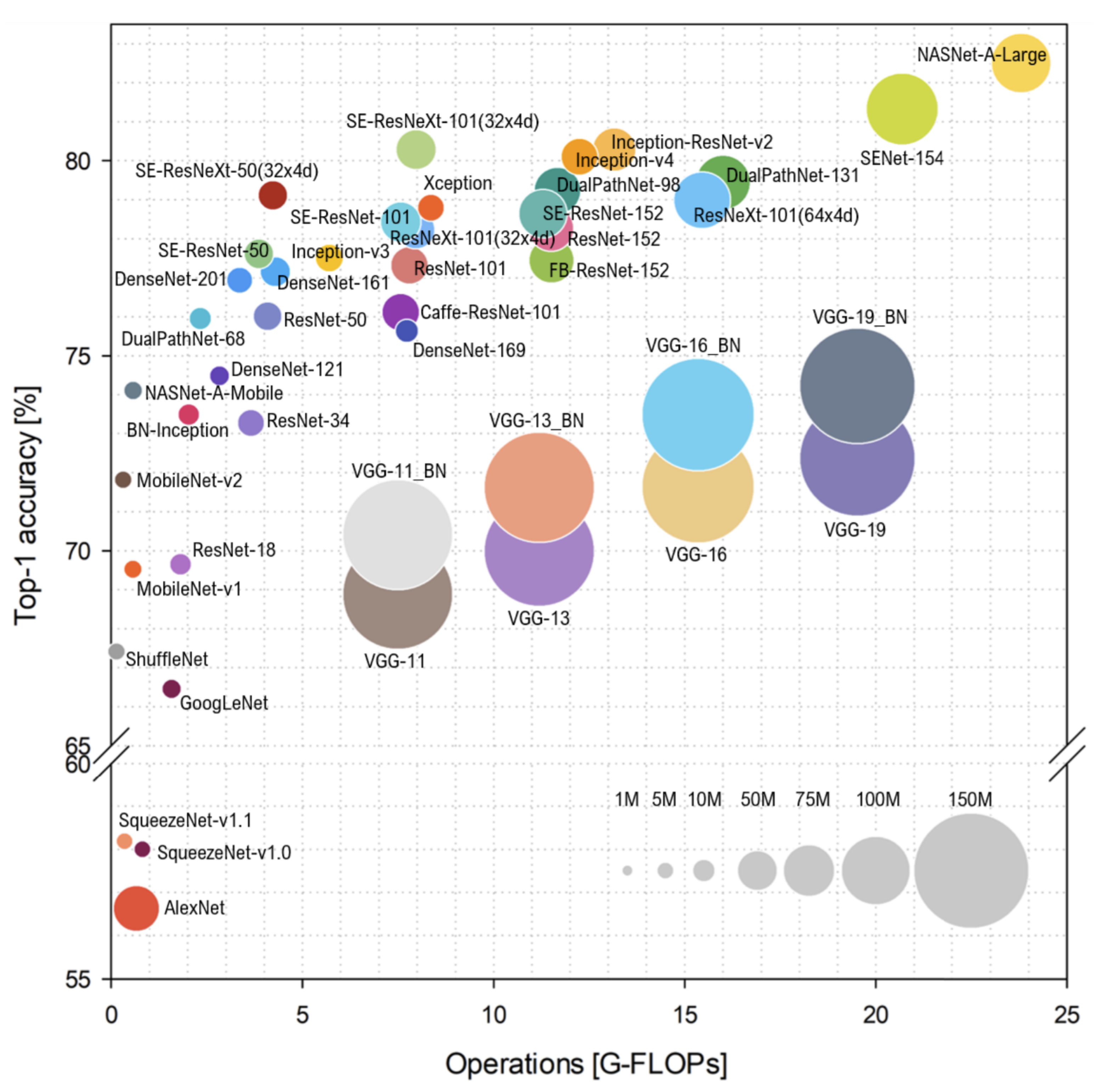
As shown in Figure 1, since the development of AlexNet [2] in 2012, which was evaluated in a 1000-class ImageNet Large-Scale Visual Recognition Competition (ImageNet-1k) [3] dataset, the literature has focused on designing more accurate and efficient networks, with regard to model complexity and size [4]. This was also enabled by the emergence of fast graphics processing units (GPUs), satisfying huge memory bandwidths and computational complexity consumed by large size DNNs. Owing to increased computing power and a sufficient amount of data being available, DNNs have evolved into wider and deeper architectures. The number of layers in DNNs can reach tens of thousands with billions of parameters [5]. Consequently, it is challenging for researchers to deploy DNNs in portable devices with limited hardware resources (e.g., memory, bandwidth, and energy). Therefore, means are urgently sought for efficiently deploying DNNs in resource-constrained edge devices (e.g., mobile phones, embedded devices, smart wearable devices, robots, drones, etc.) without detriment to the model’s performance.
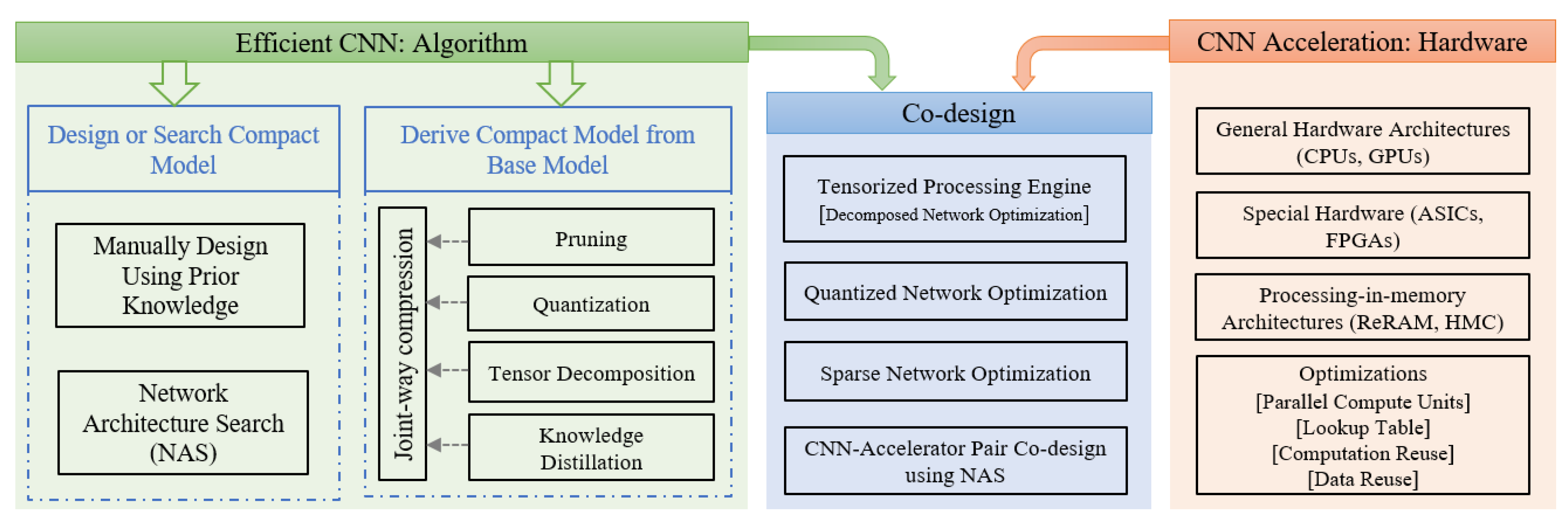
To address this problem, several efforts have been made to reduce the memory and computation requirements of DNNs while still providing optimal accuracy. In this paper, these efforts are broadly categorized into two categories: (1) design or derive an efficient CNN using a base model (e.g., quantization), and (2) directly design an efficient CNN (e.g., neural architecture search (NAS)). However, the interaction between the hardware architecture and software algorithm is also a present trend in designing efficient CNN inference systems. Figure 2 shows an overview of the efficient CNN design approaches explained in this study. We include several topics on both the algorithm and hardware design sides, focusing on the most recent work in the past few years. Our survey methodology covers from manual design algorithms to automatic algorithms, as well as sole hardware acceleration to hardware and software co-design methods.
Specifically designed CNNs with fewer parameters and small model sizes (e.g., SqueezeNet [6], ShuffleNet [7], and MobileNet [8]) achieve performances similar to larger networks (AlexNet [2] and ResNet-50 [9]). This proves that the network architecture design is crucial, which offers many opportunities for designing more efficient network architectures. However, owing to the inherent limitations of human knowledge, it is difficult to design optimal architectures based only on prior knowledge and experience. Therefore, the logical idea is to allow the algorithm to design the neural architecture automatically while minimizing human intervention. NAS approaches [10,11,12,13,14,15,16,17,18,19,20,21,22,23,24,25,26,27,28,29,30] automatically search for the optimal network design for the best possible performance under user-defined constraints, such as accuracy, model size, and inference time. Owing to the extremely large search space, the success of the NAS approach is highly dependent on an efficient and effective network architecture performance evaluation scheme.
In addition to creating a compact and efficient base model, other approaches have modified or utilized base models to reduce memory and computation costs. Those approaches can be classified into four categories: (1) pruning [10,31,32,33,34,35,36,37,38,39,40,41,42,43,44,45,46,47,48,49,50], (2) quantization [10,51,52,53,54,55,56,57,58,59,60,61,62,63,64,65,66,67,68], (3) tensor decomposition [69,70,71,72,73,74,75,76,77,78,79,80,81,82,83], and (4) knowledge distillation [84,85,86,87,88,89,90,91,92,93,94]. Among them, network pruning and quantization are well-established compression techniques that can be traced back to the early 1990s, whereas tensor decomposition and knowledge distillation are getting more attention in recent years with the evolution of deep learning.
Network pruning removes the superfluous portion of the network, ranging from the weights, filters, channels, and even the layers. The simplest form of network pruning is to remove individual parameters, which is also known as unstructured pruning. Conversely, the simultaneous removal of a group of parameters, such as neurons or filters, is known as structured pruning. A typical deep neural network applies 32-bit floating-point (FP32) precision for both training and inference. Quantization attempts to reduce the bitwidth of data flow across the neural network (e.g., replacing FP32 with 8-bit integers (INT8)), reducing the model size and simplifying operations. Extreme quantization represents the network weights and activations using 1-bits, also known as binarization [56,63,64,65,66,67,68]. The combination of quantization and pruning is the most widely used joint-way compression technique [10,51].
With the tensor being the fundamental building block and the tensor operation being a basic computation in DNNs, the number of parameters in the network can be greatly reduced by substituting the tensor with a low-rank matrix or tensor approximations. Tensor decomposition decomposes a high-rank tensor into a series of low-rank tensors, reducing both memory use and operations. It can be used in both convolutional and fully connected layers and performs well in compressing parameterized networks. The tensor decomposition model can be further compressed using pruning or quantization. The goal of knowledge distillation, another more recent efficient CNN design technique, is to train a simpler and more compressed student model that imitates the performance of a larger teacher model. The main challenge with this approach is knowing how to transfer knowledge from the teacher network to the student network. The basic knowledge distillation components are knowledge, distillation algorithms, and teacher–student architectures.
The efficient CNN design algorithms discussed above can further benefit from suitable hardware accelerator design. The resulting CNN after unstructured pruning, tensor decomposition, and quantization/binarization needs specially designed hardware architecture for maximum inference efficiency. The hardware implementation of neural networks is based on either sole hardware implementation that uses general purpose processors to joint hardware algorithm co-designs using modern hardware accelerators. The processor platforms include central processing units (CPUs), GPUs, application-specific integrated circuits (ASICs), and field-programmable gate arrays (FPGAs). The processing-in-memory (PIM)-based architectures are also being used in recent hardware implementations. The specialized hardware implementation mainly focuses on reducing data movement, energy consumption, area consumption, etc., using several dataflow and data reuse techniques. Rather than only using sole hardware implementation [95], researchers have used both algorithms and hardware to develop optimized modern neural network accelerators [96,97].
The rest of this article is organized as follows. Section 2 reviews several efficient CNN design software algorithms. These techniques range from the automatic searching of efficient networks using NAS to designing a compressed network using pruning, decomposition, quantization, and distillation depending on the base model. Section 3 highlights the hardware approaches used to accelerate the neural networks. This includes a combination of algorithm-based compression and modern hardware accelerators. Section 4 briefly discusses current efficient CNN design techniques and potential future research opportunities. Finally, we present the conclusions of the study in Section 5.
2. Efficient Convolutional Neural Networks
The efficient neural-network design approach either searches for an efficient base model from a predefined search pool or modifies the given base model to obtain the final compressed model. Network pruning, data quantization, tensor decomposition, and knowledge distillation approaches use the given base model, whereas more recent approaches, such as NAS, programmatically search for highly efficient neural network structures. In this section, we detail each of these efficient neural network design approaches.
2.1. Pruning
Network pruning is a well-known topic that can be traced back to the early 1990s [98,99]. The key idea in pruning is to remove unimportant weights, filters, channels, or even layers from the original DNN, resulting in a reduced number of memory access and computation operations. Weight or connection pruning attempts to eliminate unimportant connections from the original model, whereas more recent techniques use large-scale pruning, such as filter-pruning or channel-pruning. In general, network pruning can be categorized as (1) connection (weight) pruning, also known as unstructured pruning, and (2) filter or channel pruning, also known as structural pruning.
2.1.1. Weight Pruning
Some early works, i.e., Optimal Brain Damage (OBD) [98] and Optimal Brain Surgeon (OBS) [99], use the second derivative (Hessian matrix) of the loss function to prune each non-essential weight. The most popular early works in the deep learning era [31,32] used a three-step method to prune the weights below the threshold and demonstrated that many connections can be removed from the DNN to achieve a significant compression ratio. First, the network is trained to find important connections, then, unimportant connections are pruned, and, finally, the network is retrained to fine-tune the remaining connections. Iterative connection pruning and fine-tuning gradually produce a compressed network. Dead neurons, for which all connected weights are pruned, can also be safely dropped. Using similar-weight pruning techniques, the authors in [34,35] proved that the accuracy of large but pruned models outperforms the accuracy of their smaller but dense counterparts under identical memory footprints. However, the lottery ticket hypothesis [36] shows that dense, randomly-initialized, neural network contains subnetworks (“winning tickets”), when trained in isolation, have an accuracy comparable to original networks with a similar number of iterations. In their iterative pruning, each pruned subnetwork was trained from scratch where the weights are initialized with the same initial weights used in the original model. While the above methods use pruning in the spatial domain, Ref. [33] showed that converting spatial weights into frequency–domain weight coefficients and pruning dynamically in each iteration and different frequency bands achieves a higher compression ratio. In [31,32,33], the global magnitude threshold is set for the whole DNN, which directly affects the performance of the network, because applying the same compression rate in each layer is illogical. To overcome this problem, the methods in [37,38] use different compression ratios in each layer according to their importance in the network. The authors in [37] improved the pruning process by selectively learning the corresponding weights that have a large impact on the loss, while discarding the other weights by cutting off their gradient flow. This end-to-end training method automatically determines the per-layer sparsity ratio and does not require fine-tuning after pruning. On the other hand, another method [38], determines the layer-wise compression ratio using a mixture of Gaussian distributions (GMM) over the weight distributions in each layer. The target layers to be pruned are selected based on the quantity of small-magnitude weights in each layer estimated using GMM, and the selected layers are pruned with a specific compression rate. In another magnitude-aware pruning method [39], energy reduction, rather than only the compression ratio and accuracy loss, is also considered when determining the pruning strategy.
With connection pruning, less important weights or neurons are removed regardless of their position, resulting in an unstructured network. Although a significant number of connections can be pruned with minimal damage to the general capacity of the network, specialized software or hardware is required to support sparse matrix operations and has limited applications on the general purpose hardware.
2.1.2. Structural Pruning
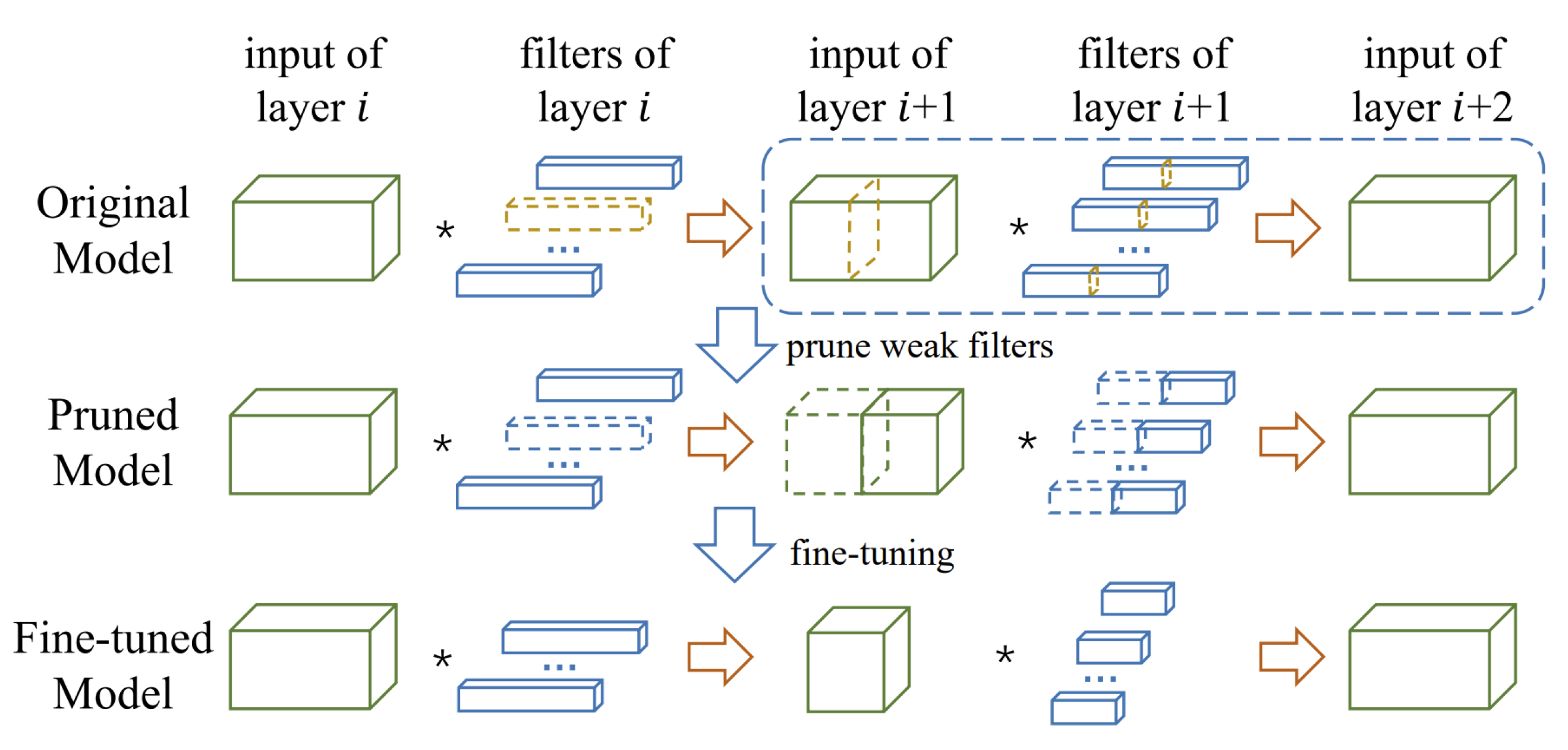
In this category, the methods aim to reduce the memory footprint by pruning entire filters, channels, or even layers. After pruning, the input and output shapes of the layers and weight matrices are changed, still permitting dense matrix operations without requiring any specialized hardware or software. Identifying the least important filter and removing it is the most popular scheme in filter pruning. Ranking the filters with certain criteria [40,41,42,43], minimizing the reconstruction errors [44,45], and finding the replaceable filters with similarity measurements [46,47] are the three main branches under this category. In [40], the filters and their connecting feature maps were removed according to their norm. Soft Filter Pruning (SFP) [41] compares both and norm criteria. They found that the performance of the norm criteria is slightly better than that of the norm criteria, because filters with large weight are preserved by norm criteria. The average percentage of zeros (APoZ) activation neurons criteria was used in [43] to delete filters with small APoZ. HRank [42] utilized the rank of feature maps to prune filters, because low-rank feature maps contain less information, and the pruned results can be easily reproduced. The NISP [45] and ThiNet [44] formulated pruning as an optimization problem. ThiNet [44] prunes the filters in the current layer and minimizes the reconstruction error in the next layer, whereas NISP [45] focuses on minimizing the reconstruction error in the “Final Response Layer” (FRL). Figure 3 shows an overview of ThiNet [44], which uses the statistics of layer to guide the pruning in layer i so that the weak channels in layer ’s input and their corresponding filters in layer i are pruned. The filter pruning via geometric median [46] and online filter clustering [47] criteria search for filters with redundancy rather than those with “relatively less” importance. In addition to filter and channel pruning, entire layer pruning methods also exist [48,49,50]. Using different criteria, selected layers from the network were removed to obtain a compact structure. These methods claim that the model obtained by layer pruning incurs even less inference time and run-time memory usage with similar accuracy than the model obtained by filter pruning methods.
Almost all the aforementioned algorithms typically follow three steps of pruning pipelines, that is, training a large model, pruning, and fine-tuning. However, based on the argument in [53], in structural pruning, fine-tuning the pruned model yields comparable or inferior performance than training the same model from scratch with randomly initialized weights. The network-slimming technique in [52] automatically identifies and prunes unimportant channels during training. This approach imposes regularization on the scaling factors in batch normalization (BN) layers to find insignificant channels (or neurons). The more recent approach in [54] also finds a compact structure by introducing the group LASSO loss to the BN layers to prune the model from scratch with randomly initialized weights.
2.2. Quantization
Quantization reduces computations by reducing the precision of the data type, instead of reducing the number of computations in the network. This minimizes the bitwidth of the data storage and flow through the deep neural network. The computation and storage of data at a lower bitwidth allows for speedy inference with reduced energy consumption. During quantization, the neural network data are restricted to a set of discrete levels that can have different distributions: uniform or non-uniform. A uniform distribution [56] with even steps is a widely used quantization scheme. A logarithmic distribution [57] is a commonly used non-uniform quantization method. Both deterministic [56] and stochastic methods were used to project high-precision data into a discrete space. The former projects data to the nearest discrete distance level, whereas, in the latter, the projection to one of the two adjacent discrete levels is determined by the probability.
Quantizing neural networks from FP32 precision to low bitwidth is a popular compression technique that can be traced back to the early 1990s [55]. There are two forms of quantization: post-training quantization [58,59] and quantization-aware training [60,61,62]. As the name suggests, post-training quantization uses the FP32 weights and activations to apply quantization after the model is fully trained. In quantization-aware training, the quantization error is considered as part of the training loss when training the model. Although post-training quantization is easy to use, quantization-aware training generally improves model’s accuracy. The researchers in [58] showed that FP32 precision parameters can be reduced to INT8 without significantly losing accuracy. Another method [59] developed a 4-bit post-training quantization approach that does not require model fine-tuning after quantization. Only INT8 was used in [60] for both the training and inference of the ResNet-50 model with a accuracy loss. The work in [61] generalizes the concept of bit precision for storing weights and activations with any number of bits instead of only INT8. The quantized version of AlexNet achieved top-1 accuracy with 1-bit weights and 2-bit activations. During training, the parameter gradients were quantized to 6-bits. The more recent quantization-aware INT8 training method [62] optimizes the computation of forward and backward passes via precisely designed loss-aware compensation and parameterized range clipping.
Binarization
The most extreme form of quantization is binarization. In binarization, the data can have only two possible values or . With binarization, heavy matrix multiplications can be replaced with simple XNOR and bitcount operations. Due to the fact that it saves significant storage and computation, binarization is a promising technique for deploying deep neural networks in resource-constrained devices. However, owing to extreme quantization, binarization inevitably suffers from heavy information loss. Simultaneously, owing to its discontinuity, optimizing a binary neural network becomes difficult. Various algorithms have been proposed to solve these issues and have achieved promising progress in recent years. BinaryConnect [63], Binarized Neural Network (BNN) [64], and XNOR-Net [65] are some of the most popular binary neural networks. Researchers have proposed heuristic and optimization problem formulations for neural network binarization.
The heuristic binarization methods in [63,64] directly binarize weights and inputs based on a predefined function. The function can be either deterministic or stochastic. The deterministic binarization function can be defined as:
where is the binarized variable, and x is the real-valued variable. Similarly, the stochastic binarization function can be defined as:
where is the “hard sigmoid” function:
BinaryConnect [63] was an early stochastic method for binarizing neural networks. The weights are binarized during both forward and backward propagation, but not during the parameter update. Later, BNN [64] extended BinaryConnect [63] networks by binarizing activations, which is recognized as the very first binary neural network. They make use of both deterministic and stochastic binarization functions to simplify hardware implementation. In contrast to BinaryConnect [63] and BNN [64], XNOR-Net [65] approximates floating-point parameters by introducing a scaling factor for the binary parameters. Therefore, the weight quantization in XNOR-Net [65] can be formulated as , where is the floating-point scaling factor for the binarized weight .
More recently, several optimization-based binarization techniques have been proposed, e.g., in [56,65,66,67,68]. The XNOR-Net [65] and DoReFa-Net [56] have attempted to reduce the quantization error during training. In DoReFa-Net [56], gradients are quantized to accelerate the training process. Instead of focusing only on local layers, other binarization techniques such as loss-aware binarization [66] and incremental network quantization [67] directly minimize the overall loss associated with the binary weights in the network. IR-Net, a more recent binarization algorithm proposed in [68], reduces the gradient error in training by using a self-adaptive error-decay estimator and is the first approach to consider information retention for both forward and backward information propagation.
2.3. Tensor Decomposition
The tensor (including the matrix) is the basic building block of, and the tensor operation is the basic computation in, DNNs. Tensor compression using tensor decomposition results in a reduced network model size and simplified tensor operations. DNN parameters in weight tensors of the convolutional layer and weight matrices of the fully connected layers are of low rank [69]. Therefore, the number of parameters in the weight matrix or tensors can be reduced by substituting them with low-rank approximations. Tensor decomposition algorithms used in DNNs can broadly be classified into two main categories: low-rank matrix decomposition and tensorized decomposition. In the following subsections, we describe them individually, in terms of their use in CNNs.
2.3.1. Low-Rank Matrix Decomposition
Matrix decomposition methods for DNNs approximate the weight matrix of a DNN layer by multiplying multiple low-rank matrices. Singular value decomposition (SVD) [70] is the most popular low-rank approximation of a matrix in which most of the information can be described by singular values. The SVD of a matrix is the factorization of A into the product of three metrics , where and are orthogonal metrics, and is a diagonal matrix with only singular values of A. A compact network model is produced by retaining only the important components of the decomposed matrices.
In [71], a simplified SVD was used to replace the original weight matrix and reduce the spatial complexity of speech recognition applications. SVD is used to decompose the product of the weight matrix and input in [72].The authors in [73] embedded sparsity with low-rank factorized matrices to achieve a better compression rate by maintaining a lower rank for unimportant neurons. Zhang et al. [74] used channel-wise SVD decomposition of the convolution layer with a kernel size of into two consecutive layers with kernel sizes and . However, it is costly to use SVD on every training step. It is also difficult to measure the rank of DNN layers during the training process. To overcome these issues, the authors of [75] proposed a SVD training technique to explicitly achieve low-rank approximations without applying SVD at every training step. Instead of compressing layers separately, Chen et al. [76] proposed a joint matrix decomposition scheme to decompose layers sharing the same structure simultaneously, in which the optimization is based on SVD.
2.3.2. Tensorized Decomposition
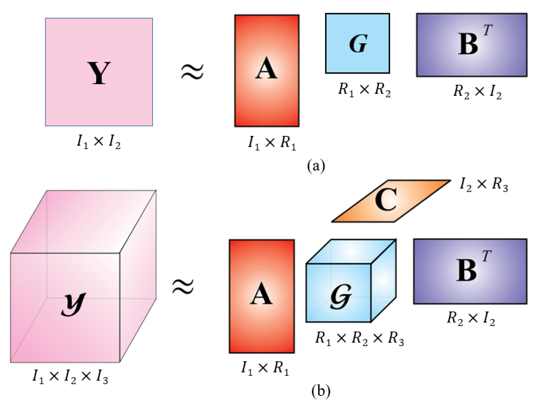
The tensor is a multiway array of data. The 2-D matrix is a second-order tensor, which is used to represent the weights of the fully connected layers. The convolutional-layer weight is represented by 4-D tensor. As the order of the tensor increases, more flexible algorithms are used to achieve a higher compression ratio, because the low-rank matrix approximation fails to utilize the tensor-based network structure. Figure 4 shows the analogy between the matrix and tensor decomposition. Recently, several tensor decomposition methods have been proposed to achieve higher compression ratios in CNNs, such as Tucker decomposition [77], CANDECOMP/PARAFAC (CP) decomposition [78,79], Tensor Train (TT) decomposition [81,82,83], and Tensor Ring (TR) decomposition [100]. CP decomposition represents a tensor by the sum of rank-1 tensors, whereas Tucker decomposition decomposes a tensor into a set of matrices and one small core tensor. Next, the TT decomposition represents a tensor in an appropriate chain of three-dimensional tensors, and, thus, it is suitable for handling higher-order tensors. TR decomposition can be viewed as an extension of TT decomposition, which is a linear combination of TT decompositions.
The authors in [77] used Tucker decomposition to compress the convolutional weight kernel of each layer using a previously determined rank. CP decomposition of the convolutional kernel into several rank-1 tensors was used in [78,79] to reduce the number of parameters and the training time. An iterative process is applied for the decomposition and fine-tuning of each convolution layer. In [79], whole convolution layers are decomposed, as apposed to [78], where only a few convolution layers underwent decomposition. Phan et al. [80] proposed a stable low-rank decomposition using a combination of both Tucker decomposition and CP decomposition, in which the core tensor from Tucker decomposition was further decomposed using CP decomposition. More advanced tensor decomposition, such as TT decomposition, has been widely used in DNN compression, particularly for recurrent neural networks (RNN) [81]. TT decomposition allows up to 1000× the parameter reduction for RNN models. However, compressing a CNN using the TT method causes significant accuracy loss. Recently, the authors in [82] proposed a TT-format DNN model suitable for a CNN not explicitly trained on the TT format. In [83], TT decomposition was adapted to compress three-dimensional CNNs (3DCNNs), and an appropriate method was proposed to select TT ranks to achieve a higher compression ratio. Another method using TR decomposition, in [100], employs a progressive genetic algorithm for optimal rank selection.
2.4. Knowledge Distillation
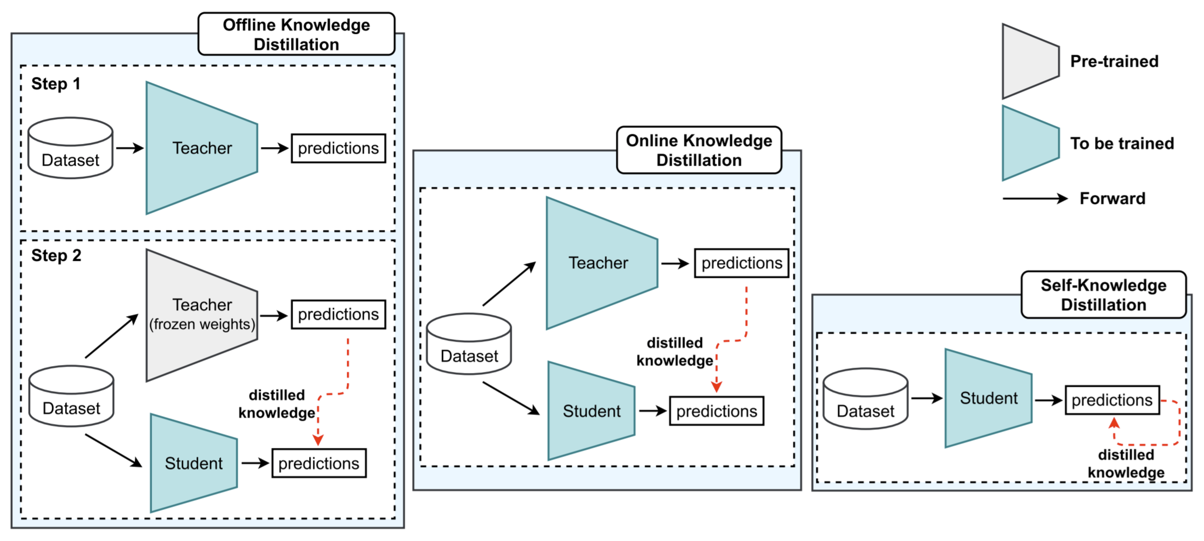
Knowledge distillation is a neural network compression technique in which a smaller or compact model (student model) is trained using information from a larger model (teacher model) about similar tasks. Knowledge distillation was first introduced by Bucilua et al. [84] and later popularized by Hinton et al. [85] for deep learning. The main challenge in knowledge distillation is how to transfer knowledge from the teacher model to the student model to achieve competitive or even better performance. In general, knowledge distillation is composed of three components: knowledge, the distillation algorithm, and the teacher–student architecture. Knowledge can take the form of logits, activations, or features from the teacher model’s intermediate layers. As shown in Figure 5, the distillation process can be offline, online, or through self-distillation. Offline distillation [86,87,88,91] distills the knowledge from the pre-trained teacher model, whereas online distillation [89,90,92] distills while the teacher and student models are being trained. In self-knowledge distillation [93,94], the student network is trained progressively using its own knowledge without requiring a pre-trained teacher model. Finally, teacher-–student architecture refers to the relationship between the selection or design structure of the student and teacher models.
The knowledge distillation methods proposed in [86,87,88] use the soft-level outputs of the teacher model to train the student model. Ensembles of teacher networks were used to train student networks in [86], in which the output distribution from multiple teacher networks via data argumentation was utilized. The authors in [87] developed a distillation method for a quantized model and claimed that quantized student networks have accuracy levels similar to their full-precision teacher model counterparts, while simultaneously achieving a high compression rate and fast inference. Nayek et al. [88] proposed a data-free method to train student networks using synthesized data responses from complex teacher networks. All the methods mentioned above use offline training and utilize the soft-level output from the teacher network. Online knowledge distillation that utilizes soft-level outputs from teacher networks is discussed in [89,90]. Jin et al. [89] proposed training the student model on different checkpoints of teacher models until the teacher models reached conversion. Knowledge Distillation via Collaborative Learning (KDCL) [90] dynamically generates high-quality soft targets using different ensemble methods for one-stage online training.
Knowledge distillation from other parts of the teacher network, such as the intermediate layers, is also possible for training student networks [91,92]. The layer-selectivity learning (LSL) method [91] proposed a two-layer selection scheme called the inter-layer Gram matrix and layered inter-class Gram matrix to select intermediate layers in both student and teacher networks for knowledge distillation. The student network was trained with an alignment loss function from the selected layers and a prediction–loss function from the teacher and student network. Another more recent ensemble-based knowledge distillation method proposed in [92] also utilizes the features from intermediate layers, in which distilled student systems and ensemble teachers are trained simultaneously without requiring a pre-trained teacher model. Many efficient neural-network architecture designs that use self-knowledge distillation have also been proposed [93,94]. The main advantage of this technique is that training a large teacher network is not necessary. Ji et al. [93] used an auxiliary self-teacher network to transfer refined knowledge for a classifier network utilizing both soft labels and intermediate feature-map distillations. In [94], the best-performing student network in past epochs was used to distill knowledge while training the current student network using an effective augmentation strategy, thus improving network generalization.
2.5. Neural Architecture Search
Efficient network design using human expert knowledge and prior experience has achieved great success in the past (e.g., SqueezeNet [6], ShuffleNet [7], and MobileNet [8]). However, because of limitations in human knowledge and expertise, the current research trend is toward automatically designing efficient neural network architectures without (or only involving minimal) human intervention. This emerging area of research into machine-aided efficient neural network architectural design is termed NAS. Unlike pruning, quantization, and tensor decomposition-based efficient network designs, NAS automatically searches for an efficient DNN without depending on the base model.
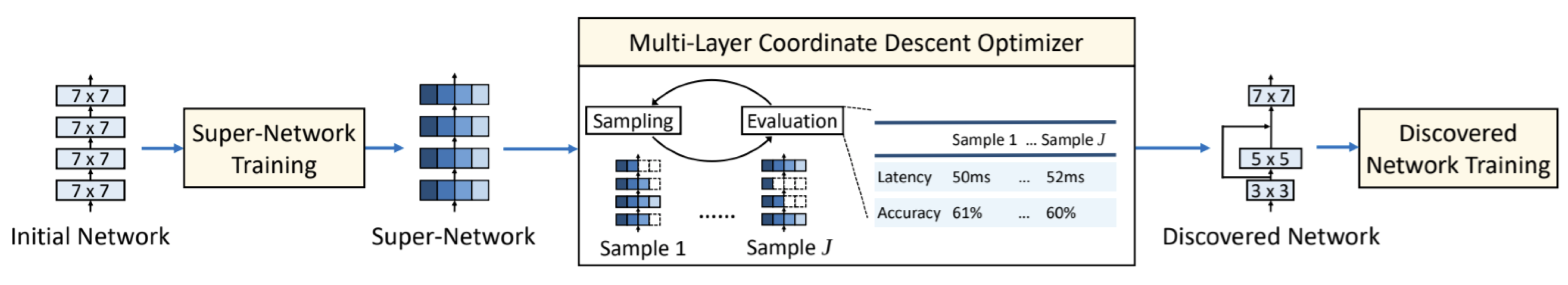
The early approach using NAS algorithms (for example, [11], Figure 6) first generated many candidate network architectures based on a predefined search-space criterion. Each network architecture was trained until convergence and ranked according to network accuracy on the validation set. This ranking can be used as feedback information to adjust the search strategy and obtain new neural architectures. This process was repeated until the termination condition was reached. Finally, the best network architecture was selected and evaluated using the test set. Using this approach, thousands of neural networks must be trained and evaluated from a vast search space, leading to tremendous computational and time costs. To address this challenge, several new NAS techniques have been proposed to improve the search space, search algorithms, and network evaluation criteria. As show in Figure 7, recent NAS approaches follow three main steps: training a super-network, training and evaluating sampled networks, and finally training the discovered network.
2.5.1. Search Space
The search space is the scope for exploring neural networks. If we search for both network elements and their connections to determine the entire network structure, the search space grows exponentially [11]. Therefore, it is necessary to restrict the search space. The search space can be restricted by searching only a finite number of small-cell structures, and the final network structure can be constructed as a sequence of repeated cells. Representative works related to the cell search space include NASNet [20], ENAS [27] and AutoDispNet [28]. For example, AutoDispNet [28] exclusively searches for two types of cells, namely, normal cells and reduction cells, in a predefined high-level network structure. ENAS [27] allows all child models to share weights, increasing the GPU processing time more than 1000 times compared to traditional NAS [11]. The major aspects of efficient network design are inference time (latency) and memory consumption, while maintaining reasonable network accuracy. MnasNet [30] is a platform-aware NAS for mobile devices that searches for networks to achieve an acceptable trade-off between latency and accuracy.
2.5.2. Search Algorithm
The search strategy governs how the search space is explored. In NAS, the generator usually produces the sample architecture, and the evaluator evaluates the performance after training. Due to the fact that an expensive training process is in the loop, the search algorithm that affects the sampling strategy plays an important role in improving the overall NAS process. The well-known search algorithms include random search (RS), Bayesian optimization (BO) [18], neuroevolution [21,22,23,24,25,26], reinforcement learning(RL) [11,20], and gradient-based optimization. Bayesian optimization [18] is one of the most popular methods for hyperparameter optimization; however, it has not been widely applied to NAS. The neural architecture obtained using RL [11] in NAS-RL [11] and MetaQnn [19] outperformed previous state-of-the-art classification accuracy in image classification tasks. Neuroevolution methods [21,22,23,24,25,26] were initially used to optimize both neural structures and weights but recently have only been used to optimize the neural structure itself. Real et al. [25] compared RL, neuroevolution with RS and concluded that RL and neuroevolution performed better than RS in terms of final test accuracy, and neuroevolution always produced better performance and smaller models.
2.5.3. Performance Evaluation Strategy
The performance estimation strategy aims to find a neural architecture that maximizes specific performance measurements to evaluate the performance of the explored model. Early NAS [11] evaluated the quality of each sampled network by training it from scratch, which is very costly. Progressive NAS [14] and ReNAS [15] speed up the evaluation step by building an accuracy predictor using data collected from training a few sample networks in the search space. Once the trained accuracy predictor is available, the search process can be guided without additional training costs. Alternatively, One-Shot NAS [12,13] reduces the evaluation costs by training a single super-net from which each sampled network inherits weights without incurring extra training costs. This weight-sharing across models in one-shot NAS has allowed major progress in reducing search costs. Although auto-designed neural networks generally perform well, they may not be suitable for hardware deployment in all edge devices, owing to their complex structures. To address this problem, recent hardware-aware NAS approaches [16,17] incorporate hardware constraints, such as inference latency, energy consumption, and memory footprints, into the search process. They also minimize the evaluation costs by training a single network that supports diverse hardware architectures.
3. Hardware Acceleration of Convolutional Neural Networks
Since the beginning of the past decade, the development of DNN solutions has accelerated in many applications. This was enabled by the advent of fast GPUs, which could satisfy the huge memory bandwidth and computational complexity caused by the ever-increasing size of DNNs. The deep learning solutions not only limit their applications to heavy computing machines, but there is also growing interest in deploying DNNs in edge devices with limited hardware resources and energy. The hardware solutions for DNNs development and deployment range from general purpose architectures (CPUs and GPUs) to spatial architectures (FPGA and ASCI).
The multiply-and-accumulate (MAC) operation is the fundamental component in both the fully connected and convolution layers, which can be parallelized easily to achieve a high inference speed. The hardware accelerator can either be a conventional hardware optimization with enhanced compute parallelism or modern accelerators that combine both hardware and software design capabilities. Recent advancements in developing efficient DNNs using software solutions provide promising performance with reduced memory and computing operations. DNN acceleration that uses hardware-software co-design is the current trend in developing efficient DNN applications. In the following subsections, we first discuss the available temporal and spatial hardware architectures that are suitable for DNNs. Next, we briefly review processing in memory (PIM)-based architectures and their corresponding DNN accelerators. Thereafter, we will focus on the codesign of DNN accelerators that leverage the capabilities of both hardware architecture and compression algorithms. Finally, as a case study, we present some well-known representative DNN accelerators for practical applications.
3.1. Temporal and Spatial Hardware Architectures
In general, CPUs and GPUs use temporal architectures, whereas the ASIC-and FPGA-based designs use spatial architectures. Although they have similar computational structures with multiple processing units, they differ in several aspects, such as the control units, memory structures, and dataflows. The temporal architecture uses a large number of ALUs as processing units with centralized control. The ALUs in the temporal architecture do not have their own local memory and cannot communicate with each other directly. However, in spatial architectures, ALUs can have their own local memory and control logic, also known as processing elements (PEs). PEs are interconnected in a processing chain so that they can pass data and directly communicate with each other, as opposed to ALUs, in temporal architectures.
For parallelism, CPUs use the single-instruction multiple-data (SIMD) model and GPUs use the single-instruction multiple-thread (SIMT) execution model. On temporal platforms, the FC and convolution layers in the DNN are primarily mapped to matrix multiplication. Software libraries such as OpenBLAS and Intel MKL for CPUs, and cuBLAS and cuDNN for GPUs are available for the optimization of matrix multiplications. As these architectures are general purpose and designed to support a wide range of applications, users are less likely to find such hardware architectures specially designed exclusively for DNN applications.
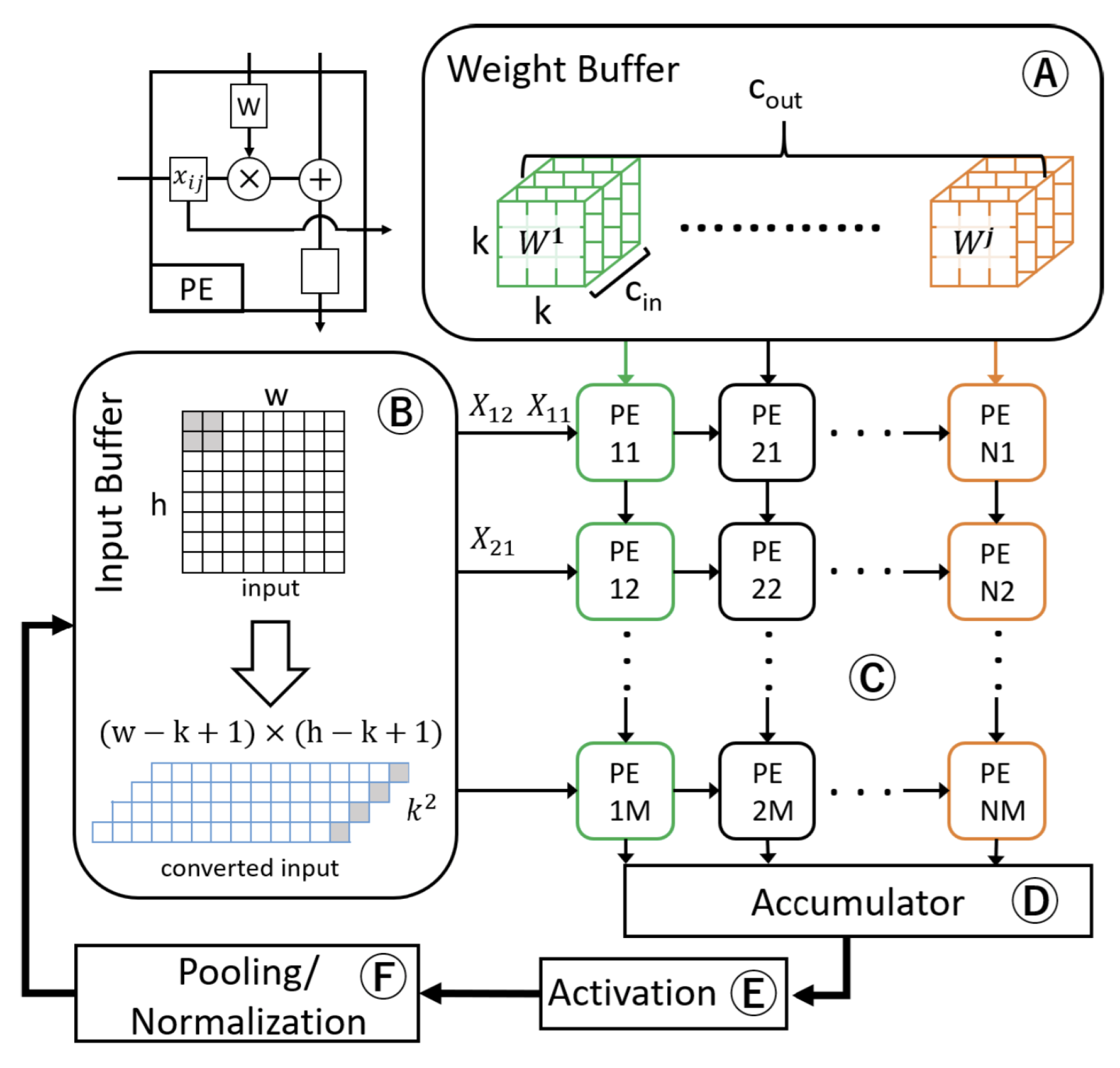
For DNNs accelerators with spatial architecture implemented on an ASCI or FPGA, the bottleneck is in memory access. An array of PEs with a small local buffer and a global buffer is used to reduce data access from the DRAM. As show in Figure 8, the two-dimensional network of the PE array performs dataflow processing in an orchestrated network-on-chip (NoC), which enables direct-message passing between PEs. When performing convolution, for each MAC, data flows through PE arrays, enabling direct-message passing, thus increasing data reuse and decreasing the memory bandwidth. Three types of data reuse (convolution, filter weight, and input feature map) can be exploited in CNNs by storing the data in the local memory hierarchy. Based on the dataflow characteristics of different DNNs’ accelerator designs, they are classified into four categories: (a) weight-stationary (e.g., TPU [95] and [101]), (b) input-stationary (e.g., SCNN [102]), (c) output-stationary (e.g., Origami [103] and [104]), and (d) row-stationary (e.g., Eyeriss [105] and Eyeriss-v2 [106]).
As shown in Figure 8, the weight-stationary dataflow stores the weight in the register file (RF) of the PE, thus exploiting filter-weight reuse and convolution reuse, while inputs and the partial sum move between PEs. The input-stationary dataflow structure stores the input feature map values in an array, and convolution is performed by passing the weight value to the array in the PE. The accumulations of the partial sum are kept in each PE until the final sum is reached in the output-stationary dataflow, minimizing the read and write operations of partial sums. The input activation and filter weights are distributed across the PE arrays, thus reusing the convolution. Finally, row-stationary dataflow architectures jointly maximize the reuse of the filter weights, input activations, and partial sums. The convolution operation between one input row and the weight row is performed in the same PE. Among the dataflow architectures mentioned above, the row-stationary dataflow has the lowest energy consumption. For instance, Eyeriss [105] is a popular DNN accelerator using row-stationary dataflow.
3.2. Processing-in-Memory (PIM) Architectures
The energy consumption in FPGAs and ASIC architectures is mostly dominated by data movement between memory and processing elements because of the limited on-chip memory and data transfer bandwidth. Several efforts have been made to solve this issue using new memory technologies such as dynamic random access memory (DRAM), resistive random access memory (ReRAM) [107], and hybrid memory cube (HMC) [108] to enable the direct integration of the processing engine and memory storage known as PIM. The PIM technique minimizes data movement by performing some computations within the memory itself, thus reducing penalties incurred by memory accesses. Some representative studies using DRAM, ReRAM, and HMC-based PIM architectures for DNNs acceleration are DrAcc [109], PRIME [110] and PattPIM [111], and Neurocube [112], respectively.
The DrAcc [109] accelerator is designed for ternary weight CNNs by performing in-DRAM bit operations that can achieve almost 84 frames per second (FPS) inference speed at 2 W of power consumption. In ReRAM, which is an emerging nonvolatile memory, the ReRAM array can be used as a computation engine for matrix-vector multiplication. PRIME [110] replaces DRAM with ReRAM, which is used for both storage and computation. It uses a ReRAM array configured for a 4-bit multilevel cell computation or 1-bit single-level cell storage. Recently, in PattPIM [111], the ReRAM crossbar array was utilized for space compression and computation reuse by exploiting the weight pattern repetition characteristics in a CNN. An intra-processing engine pipeline was designed to enhance parallel computing within the ReRAM memory itself. Although the ReRAM-based PIM technique seems to have great potential in DDN accelerator design, the actual fabrication of large ReRAM arrays is still a challenging research task. In another memory structure, HMC, also known as 3-D memory, DRAM is vertically stacked on top of the chip, enabling low latency and high memory bandwidth. Neurocube [112] consists of a cluster of processing engines, in which the processing engine clusters can access multiple memory channels (vaults) of the HMC’s DRAM in parallel. This integrates the processing engine into the logic die of the HMC to bring MAC computing and memory closer.
3.3. Co-Design of Hardware Architecture and Compression Algorithm
CNN compression algorithms such as pruning and quantization are widely used to obtain efficient CNN structures, and the hardware acceleration of the CNN can be optimized further by designing a hardware accelerator, particularly for efficient CNN structures obtained via compression algorithms. Network pruning, specifically unstructured pruning, helps to reduce off-chip memory access by significantly removing unimportant weights or activations [31,32,33,34,35,36,37,38,39]. Similarly, quantization can help reduce computation and memory storage by operating with low-bit precision [10,51,52,53,54,55,56,57,58,59,60,61,62,63,64,65,66,67,68]. In addition, hardware-aware NAS techniques have been developed to improve the performance of CNNs automatically on target hardware by considering inference latency, energy consumption, and memory footprints [16,17,30,101,113].
As discussed in Section 2.1.1, many weights or connections in CNNs can be pruned to zero with or without minimal accuracy loss, resulting in highly sparse network. The sparse hardware accelerator can be designed for such sparse networks providing room for saving large amounts of energy and storage. Cambricon-X [114] is an early sparse CNN accelerator skipping MAC operations for zero weights. The required weights are accessed by the PE using index of the weights that are stored in sparse format. Later, Cambricon-S [115] improved the weight indexing overhead by addressing memory access irregularities using a cooperative hardware–software approach. The SCNN in [102] supported the processing of a convolutional layer in a compressed domain by exploiting both zero-valued weights arising from pruning and zero-valued activation from having a common ReLU operator during inference. The input stationary dataflow is used to maintain the weights and activations in the compressed domain, eliminating unnecessary data transfer and storage. A drawback of this method is that it results in massive write-back traffic and supports only the convolutional layer. Eyeriss-v2 [106] also processes nonzero weights and activations in the compressed domain of a sparse network by adapting the Eyeriss-like row stationary dataflow [105] to avoid memory access overhead. SNAP [116] uses an associative index-matching search to find matching non-zero input activations and weight kernels. It supports a general convolution, pointwise convolution, and fully connected layers. Two-level partial sum reduction (PE level and core level) is used to process the output neurons, reducing write-back traffic and memory access.
As discussed in Section 2.2, quantized architectures aggressively reduce the bit width of the weight and activations up to 1-bit to obtain an ultra-high inference speed with a certain degree of accuracy loss. The special purpose hardware accelerator that utilizes both variable-bitwidth arithmetic (e.g., Stripes [117], BitFusion [118], UNPU [119], and BitBlade [120]), and fixed-bitwidth arithmetic (e.g., [121], and YodaNN [122]), has been developed for quantized neural networks. If weights and activations are both binarized or ternarized, the MAC operations can be replaced with simple XNOR and pop-count operations. The architectures with fixed-bitwidth arithmetic, such as [121] and YodaNN [122], are similar to the hardware accelerators used for uncompressed CNNs, but complex MAC operations are replaced with simpler lower-bit logic. Quantized CNNs with variable bitwidth representation can achieve better results with a reduced model size [56]. Stripes [117] used the AND logic operation and shifted accumulations with bit-serial computations, where the bit width of the weights is fixed, and variable bitwidth is used for activations. Similar to Stripes [117], UNPU [119] also used bit-serial computation, but a 16-bit fixed-bitwidth was used for activations and a 1-bit to 16-bit variable bitwidth was used for filter weights. BitFusion [118] dynamically fuses an array of bit-level PEs to match the bitwidth of different DNN layers and minimize computation and communication with no loss of accuracy. The recently proposed BitBlade [120] further improved the BitFusion [118] accelerator by replacing shift-add logic with bitwise summation. Several binary or ternary neural networks have also been implemented in FPGA specialized architectures [96,123,124,125]. A quantized neural network with 3-bit features was implemented in the Zynq UltraScale+ FPGAs and ARM NEON CPU processor by [123]. However, in their accelerator design, the first and last layers of the Tiny-YOLO network used 8-bit arithmetic operations. FINN [124] is another BNN inference framework implemented in an FPGA, in which all fully connected, convolutional, and pooling layers are binarized. The more recent reconfigurable BNN accelerator proposed in [125] applies adaptive parallelism based on the target-layer parameters and achieved 9.69 times higher area—speed efficiency than traditional FPGA implementations. In addition to specialized hardware, quantized neural networks (especially INT8) are also widely supported in general purpose ARM CPU hardware architectures (e.g., ARM Cortex-A75 and Mali-G76). These ARM CPUs support CNN acceleration, enabling INT8 matrix operations in ARM NEON, which is an advanced SIMD architecture extension.
In addition to network quantization and pruning, tensor decomposition is another compression algorithm for CNN acceleration. Although the resultant networks are still dense after tensor decomposition and can run on general purpose hardware, in some cases, such as TT decomposition, hardware support is needed to further improve network efficiency. In the TIE [97] hardware accelerator, expensive tensor reshape and transpose operations are implemented at almost zero cost by partitioning the working SRAM into multiple groups with a well-designed data selection mechanism. Recently, Ref. [126] accelerated the TT decomposition process using an algorithm–hardware co-design with a customized hardware architecture. The SVD computation pattern within each TT decomposition iteration is adjusted to reduce the overall computational cost.
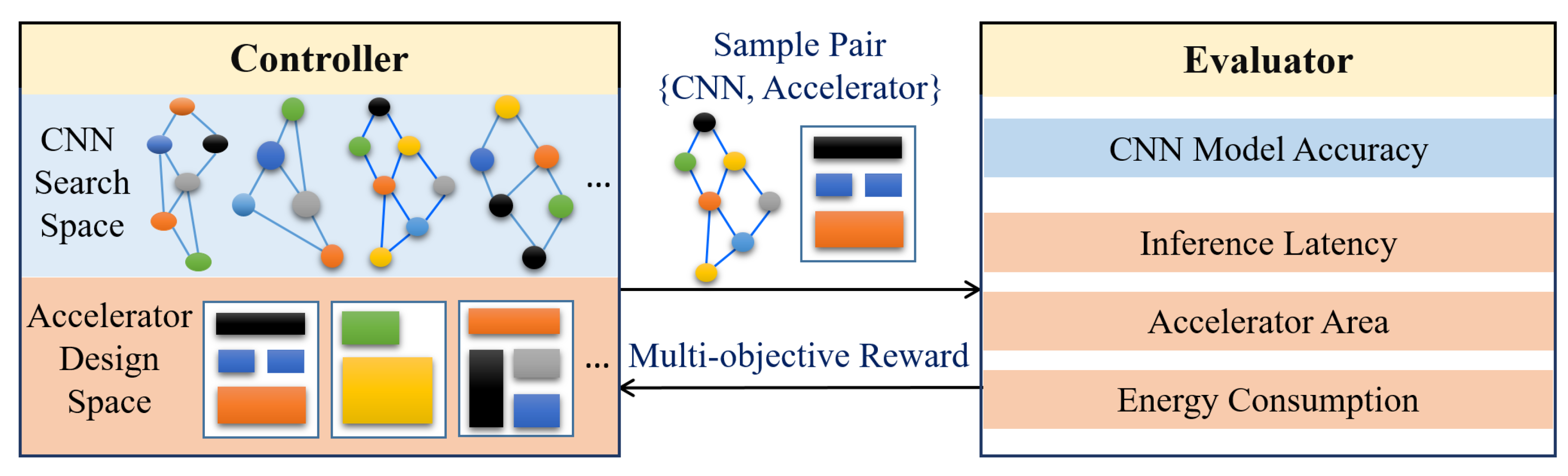
More recently, as shown in Figure 9, NAS techniques for searching efficient CNNs also integrated hardware accelerator design considerations into the search loop to jointly search for the model–accelerator pair with the best accuracy and efficiency. MnasNet [30] searched for an efficient CNN for mobile devices in which model latency was explicitly incorporated into the main objective to achieve a good trade-off between model accuracy and latency. Similarly, Ref. [17] also included hardware platform constraints while searching for an efficient CNN. The Codesign-NAS [113] moves one step further and searches for a CNN–accelerator pair for the best accuracy and efficiency. A recently proposed polynomial regression-based NAS [127] technique searches through different combinations of quantization and scaling factors of the model architecture to satisfy the target accuracy. Next, for the model with optimized and , they searched through different combinations of MACs and PEs to design an optimal hardware accelerator regarding energy consumption. In general, the hardware-aware NAS techniques proposed in [17,30] only explore the NAS space while assuming a fixed hardware architecture design, while the techniques proposed in [113,127] simultaneously explore both the architecture search space and hardware design space to find the best model–accelerator pairs that maximize both inference accuracy and hardware efficiency.
3.4. Practical Applications: Case Study
In this section, we survey the practical applications of temporal and spatial hardware architectures. There are various implementation technologies, including high-performance GPUs/CPUs, CPU-controlled FPGA solutions, and specialized accelerators. One of the most successful cases is the general-purpose graphics processor architecture developed by NVIDIA. GPUs, originally developed to support video games, are now increasingly being used for deep learning within Tesla, Fermi, Kepler, Maxwell, Pascal, Volta, Turing, and Ampere architectures. The NVIDIA cards with CUDA libraries are supported by the widest variety of deep learning applications. AMD GPUs, such as the RADEON series, are also effective regarding computational performance and memory bandwidth, but, because of lacking community, software, and tensor cores, they will probably not be able to compete with NVIDIA GPGPU solutions. In many servers and workstations, NVIDIA solutions, such as DGX systems, are utilized to train deep learning models. Google has released four versions of its tensor processing unit (TPU) for data-center deployment. The TPU, initially only intended for inference, was soon improved for both training and inference. As a GPU-based accelerator it is a generalized structure and, therefore, is not optimized for resource-constrained contexts.
Several smartphone vendors, such as Apple (A-series), Huawei (Kirin), and Samsung (Exynos), embed GPU-based neural engines or so-called neural processing units (NPUs) in their smartphones to enable inference-based tasks. Systems in this category are also aimed at autonomous vehicles, robots, and UAVs. They have several ARM cores that are mated with GPGPU cores, such as the NVIDIA Jetson-TX1/TX2, Nano, and NVIDIA Xavier. For low-power devices, the edge TPU is a small ASIC designed by Google that provides high-performance AI/ML inference. ARM Ethos, CEVA NeuPro, and Hailo AI chips are also suitable for embedded platforms or edge devices. The use of FPGAs for neural networks has been studied primarily in university and industry research laboratories. For example, Bruhnspace, in collaboration with Unibap AB and Mälardalen University, provides experimental packages of ROCm with AMD APUs support for research purposes. One of the Intel solutions pairs an Intel Xeon CPU with a reconfigurable Alteran Arria FPGA. Microsoft Brainwave is a programmable Intel Stratix FPGA that was deployed as part of the Catapult project. Although a few have announced or are offering products with spatial architecture, many architectures and software have been actively researched in the CPU-–FPGA–ASIC paradigm.
4. Discussions
Several algorithm-based solutions and hardware acceleration approaches for designing efficient CNNs are presented in this paper, including hardware–software codesign. The intuitive means of designing the best solution is to use a suitable compression algorithm to obtain a light-weight CNN and design the corresponding hardware architecture with optimal energy savings. Various matrices should be considered for measuring the strengths and weaknesses of the proposed efficient CNN accelerator design technique, which includes model accuracy, energy consumption, latency, and cost. However, there is no golden rule for selecting which compression algorithm and hardware architecture design will produce the best results in terms of the above matrices. Choosing a suitable method strictly depends on the specific applications and requirements. In this section, we discuss the efficient CNN’s design approaches based on the strengths and weaknesses of both the hardware and software solutions, including potential research opportunities.
The most common and widely used CNN compression algorithms fall into the categories of pruning and quantization. In many cases, pruning and quantization are used jointly to obtain the optimal compression ratio [10,51]. Weight pruning and connection pruning result in unstructured networks, whereas filter and channel pruning result in structured networks. The advantages of weight pruning and connection pruning are that they can achieve large compression ratios with reasonable performance but require a specialized hardware accelerator design for deployment. Hardware-accelerator-skipping MAC operations for zero weights and input activations with suitable data reuse and dataflow schemes can reduce energy and storage [102,106,114,115]. Conversely, after structural pruning, networks can still run in general purpose hardware as the original structure of the network will not be distorted. However, it is difficult to maintain the accuracy, because entire filters or channels will be removed, causing some important parameters to be lost. Recent research proves that, rather than following the conventional approach of pruning (training → pruning → fine-tuning), in structural pruning, training the pruned network structure from scratch with randomly initialized weights will produce even better performance [52,53,54]. Quantization, on other other hand, reduces the bit width of the data flowing through the network, thus enabling reduced storage and simplified computations. Non-uniform quantization better captures the original information of the model but requires specialized hardware for deployment, whereas uniform quantization is more common because of its simplicity and ability to run in general hardware architectures. However, uniform quantization may reduce performance. Mixed-precision quantization proved to be better regarding both accuracy and hardware efficiency with reduced memory storage [117,118,119,120]. In applications where accuracy is not critical, extreme quantization, such as binarization, can benefit from deployment on extremely low-cost hardware. Binarization of the CNN proved to perform reasonably well in image classification tasks, but other applications, such as object detection and semantic segmentation, are still open research challenges.
Model compression using tensor decomposition has promising potential, but its success is currently limited to the compression of RNN models [81]. CNN compression using tensor decomposition suffers significant accuracy loss, even for small compression ratios. For example, in the recently proposed TR decomposition method [100], a 1.9% of accuracy compromise achieves only a 5.8% compression ratio. The main problem lies in training the tensor-decomposed CNN models. Therefore, to utilize the potential of tensor decomposition in the compression of CNN, more focus should be given to the efficient training and development of more general decomposition methods.
Another CNN compression algorithm, namely knowledge distillation, is applicable when the training dataset is insufficient. The resulting compressed student model benefits from the teacher model through knowledge transfer. The advantage of compression using this technique is that, without any special hardware support, a significant compression ratio can be achieved; thus, it is applicable even in general purpose hardware architectures. Knowledge distillation can be used in combination with NAS further to improve the computational cost and parameters in the resulting compressed student network [128].
Traditional NAS approaches suffer from high computational costs and training times, because each network sampled from a vast search space is trained from scratch and evaluated to obtain the final compressed network architecture [11]. A recent approach solves this issue by training a single super network, in which each sampled network shares the weights from the supernet without requiring retraining for performance evaluation [12,29]. More recently, researchers have taken a step toward simultaneously automating CNN compression and hardware accelerator design by using NAS to search for CNN–accelerator pairs [113,127]. As diverse hardware architectures ranging from general proposals to spatial accelerators are becoming publicly available, NAS research should focus on moving in the same direction to develop a more general framework to design efficient CNN–accelerator pairs, producing maximum efficiency at minimum cost.
Hardware–software co-design benefits from exploiting the compression techniques in hardware accelerator design. Section 3.3 reviews several techniques employed in the co-design of an efficient CNN accelerator. Joint-way compression with quantization and sparsification appears to be the most common technique, even in hardware accelerator design. While designing the final CNN accelerator, several matrices should be considered, including model accuracy, model architecture, number of MACs, memory requirement, power and energy consumption, latency, and cost. Accelerator designs that use emerging memory technology seem to have great potential but must still address several research challenges. This can be one of the potential research opportunities for both academic and industrial CNNs applications.
5. Conclusions
In this study, we provide a comprehensive survey of efficient CNN design and deployment techniques, with a focus on current research trends. Both algorithm and hardware architecture design cover diverse topics. We have presented the most recent progress in all aspects of efficient CNN designs and discussed their weaknesses, strengths, and potential research opportunities. Pruning, quantization, and tensor decomposition are the most popular and well-established neural network compression algorithms, whereas knowledge distillation and NAS are popular in the era of deep learning. The most advanced and efficient CNN design approach, NAS, focuses on automatically designing neural architectures in combination with a target hardware accelerator that overcomes the weaknesses of traditional manual design approaches using limited human expert knowledge. Hardware architecture design also ranges from general purposed solutions to specialized architectures, including processing-in-memory architectures. The selection of the best compression technique, along with suitable hardware deployment, depends on several evaluation matrices, including accuracy, energy, and cost, along with the target application and user requirements.
Author Contributions
Conceptualization, S.-h.K. and D.G.; formal analysis, D.G.; investigation, S.-h.K. and D.G.; data curation, D.G.; writing—original draft preparation, D.G., D.K. and S.-h.K.; writing—review and editing, D.G. and S.-h.K.; supervision, S.-h.K.; funding acquisition, S.-h.K. All authors have read and agreed to the published version of the manuscript.
Funding
This work was supported by a National Research Foundation of Korea (NRF) grant funded by the Korean government(MSIT) (No. NRF-2021R1A4A1032252).
Acknowledgments
We appreciate our reviewers and editors for their precious time in providing valuable comments and improving our paper. In surveying efficient CNN architectures and hardware acceleration, we are deeply grateful again for all the researchers and their contributions to our science.
Conflicts of Interest
The authors declare no conflict of interest.
References
- LeCun, Y.; Bengio, Y.; Hinton, J. Deep Learning. Nature 2015, 521, 436–444. [Google Scholar] [CrossRef]
- Krizhevsky, A.; Sutskever, I.; Hinton, J. Imagenet Classification with Deep Convolutional Neural Networks. In Proceedings of the Advances in Neural Information Processing Systems, Lake Tahoe, NV, USA, 3–6 December 2012; pp. 1097–1105. [Google Scholar]
- Deng, J.; Dong, W.; Socher, R.; Li, L.J.; Li, K.; Li, F.F. ImageNet: A Large-scale Hierarchical Image Database. In Proceedings of the IEEE Conference on Computer Vision and Pattern Recognition (CVPR), Miami, FL, USA, 20–25 June 2009. [Google Scholar]
- Bianco, S.; Cadene, R.; Celona, L.; Napoletano, T. Benchmark Analysis of Representative Deep Neural Network Architectures. IEEE Access. 2018, 6, 64270–67277. [Google Scholar] [CrossRef]
- Xiao, L.; Bahri, Y.; Sohl-Dickstein, J.; Schoenholz, S.; Pennington, J. Dynamical isometry and a mean field theory of cnns: How to train 10,000-layer vanilla convolutional neural networks. In Proceedings of the International Conference on Machine Learning (ICML), Stockholm, Sweden, 10–15 July 2018. [Google Scholar]
- Iandola, F.; Han, S.; Moskewicz, M.-G.; Ashraf, K.; Dally, W.; Keutzer, K. Squeezenet: Alexnet-level Accuracy with 50× fewer Parameters and <0.5 MB Model Size. arXiv 2017, arXiv:1602.07360. [Google Scholar]
- Zhang, X.; Zhou, X.; Lin, M.; Sun, J. ShuffleNet: An Extremely Efficient Convolutional Neural Network for Mobile Devices. In Proceedings of the IEEE Conference on Computer Vision and Pattern Recognition (CVPR), Salt Lake, UT, USA, 19–21 June 2018. [Google Scholar]
- Howard, A.G.; Zhu, M.; Chen, B.; Kalenichenko, D.; Wang, W.; Weyand, T.; Andreetto, M.; Adam, H. MobileNets: Efficient Convolutional Neural Networks for Mobile Vision Applications. arXiv 2017, arXiv:1704.04861. [Google Scholar]
- He, K.; Xiangyu, Z.; Shaoqing, R.; Jian, S. Deep Residual Learning for Image Recognition. In Proceedings of the IEEE Conference on Computer Vision and Pattern Recognition (CVPR), Las Vegas, NV, USA, 27–30 June 2016. [Google Scholar]
- Wang, T.; Wang, K.; Cai, H.; Lin, J.; Liu, Z.; Wang, H.; Lin, Y.; Han, S. APQ: Joint Search for Network Architecture, Pruning and Quantization Policy. In Proceedings of the IEEE Conference on Computer Vision and Pattern Recognition (CVPR), Virtual, 14–10 June 2020. [Google Scholar]
- Zoph, B.; Li, Q.-V. Neural Architecture Search with Reinforcement Learning. In Proceedings of the 5th International Conference on Learning Representations (ICLR), Toulon, France, 24–26 April 2017. [Google Scholar]
- Brock, A.; Lim, T.; Ritchie, J.M.; Weston, N. Smash: One-shot model architecture search through hypernetworks. In Proceedings of the 6th International Conference on Learning Representations (ICLR), Vancouver, BC, Canada, 30 April–3 May 2018. [Google Scholar]
- Zhang, M.; Li, H.; Pan, S.; Chang, X.; Zhou, C.; Ge, Z.; Su, S. One-Shot Neural Architecture Search: Maximising Diversity to Overcome Catastrophic Forgetting. IEEE Trans. Pattern Anal. Mach. Intell. 2021, 43, 2921–2935. [Google Scholar] [CrossRef]
- Liu, C.; Zoph, B.; Neumann, M.; Shlens, J.; Hua, W.; Li, L.J.; Li, F.-F.; Yuille, A.; Huang, J.; Murphy, K. Progressive neural architecture search. In Proceedings of the European Conference on Computer Vision (ECCV), Munich, Germany, 8–14 September 2018. [Google Scholar]
- Xu, Y.; Wang, Y.; Han, K.; Tang, Y.; Jui, S.; Xu, C.; Xu, C. Renas: Relativistic evaluation of neural architecture search. In Proceedings of the IEEE/CVF Conference on Computer Vision and Pattern Recognition (CVPR), Virtual, 19–25 June 2021. [Google Scholar]
- Cai, H.; Gan, C.; Wang, T.; Zhang, Z.; Han, S. Once-for-all: Train one network and specialize it for efficient deployment. In Proceedings of the International Conference on Learning Representations (ICLR), Virtual, 26 April–1 May 2020. [Google Scholar]
- Xia, X.; Xiao, X.; Wang, X.; Zheng, M. Progressive Automatic Design of Search Space for One-Shot Neural Architecture Search. In Proceedings of the IEEE/CVF Winter Conference on Applications of Computer Vision (WACV), Waikoloa, HI, USA, 4–8 January 2022. [Google Scholar]
- Bergstra, J.; Yamins, D.; Cox, D. Making a science of model search: Hyperparameter optimization in hundreds of dimensions for vision architectures. In Proceedings of the 30th International Conference on Machine Learning (ICML), Atlanta, GA, USA, 16–21 June 2013. [Google Scholar]
- Baker, B.; Gupta, O.; Naik, N.; Raskar, R. Designing neural network architectures using reinforcement learning. arXiv 2016, arXiv:1611.02167. [Google Scholar]
- Zoph, B.; Vasudevan, V.; Shlens, J.; Le, Q.V. Learning transferable architectures for scalable image recognition. In Proceedings of the IEEE/CVF Conference on Computer Vision and Pattern Recognition (CVPR), Salt Lake, UT, USA, 18–22 June 2018. [Google Scholar]
- Stanley, K.O.; Miikkulainen, R. Evolving neural networks through augmenting topologies. Evol. Comput. 2002, 10, 99–127. [Google Scholar] [CrossRef]
- Real, E.; Moore, S.; Selle, A.; Saxena, S.; Suematsu, Y.L.; Tan, J.; Le, Q.V.; Kurakin, A. Large-scale evolution of image classifiers. In Proceedings of the 34th International Conference on Machine Learning (ICML), Sydney, Australia, 6–11 August 2017. [Google Scholar]
- Suganuma, M.; Shirakawa, S.; Nagao, T. A genetic programming approach to designing convolutional neural network architectures. In Proceedings of the Genetic and Evolutionary Computation Conference (GECCO), Berlin, Germany, 15–19 July 2017. [Google Scholar]
- Liu, H.; Simonyan, K.; Vinyals, O.; Fernando, C.; Kavukcuoglu, K. Hierarchical representations for efficient architecture search. In Proceedings of the 6th International Conference on Learning Representations (ICLR), Vancouver, BC, Canada, 30 April–3 May 2018. [Google Scholar]
- Real, E.; Aggarwal, A.; Huang, Y.; Le, Q.V. Aging Evolution for Image Classifier Architecture Search. In Proceedings of the AAAI Conference on Artificial Intelligence, Honolulu, HI, USA, 27 January–1 February 2019. [Google Scholar]
- Miikkulainen, R.; Liang, J.; Meyerson, E.; Rawal, A.; Fink, D.; Francon, O.; Raju, B.; Shahrzad, H.; Navruzyan, A.; Duffy, N.; et al. Evolving deep neural networks. In Artificial Intelligence in the Age of Neural Networks and Brain Computing; Academic Press: Cambridge, MA, USA, 2019; pp. 293–312. [Google Scholar]
- Pham, H.; Guan, M.; Zoph, B.; Le, Q.; Dean, J. Efficient neural architecture search via parameters sharing. In Proceedings of the 35th International Conference on Machine Learning (ICML), Stockholm, Sweden, 10–15 July 2018. [Google Scholar]
- Saikia, T.; Marrakchi, Y.; Zela, A.; Hutter, F.; Brox, T. Autodispnet: Improving disparity estimation with automl. In Proceedings of the IEEE/CVF International Conference on Computer Vision (ICCV), Seoul, Korea, 17 October–2 November 2019. [Google Scholar]
- Yang, T.J.; Liao, Y.L.; Sze, V. Netadaptv2: Efficient neural architecture search with fast super-network training and architecture optimization. In Proceedings of the IEEE/CVF Conference on Computer Vision and Pattern Recognition (CVPR), Virtual, 19–25 June 2021. [Google Scholar]
- Tan, M.; Chen, B.; Pang, R.; Vasudevan, V.; Sandler, M.; Howard, A.; Le, Q.V. MnasNet: Platform-Aware Neural Architecture Search for Mobile. In Proceedings of the IEEE/CVF Conference on Computer Vision and Pattern Recognition (CVPR), Seoul, Korea, 27 October–30 November 2019. [Google Scholar]
- Han, S.; Pool, J.; Tran, J.; Dally, W.J. Learning both weights and connections for efficient neural networks. In Proceedings of the 28th International Conference on Neural Information Processing Systems (NIPS), Montréal, QC, Canada, 7–10 December 2015. [Google Scholar]
- Han, S.; Mao, H.; Dally, W.J. Deep Compression: Compressing Deep Neural Networks with Pruning, Trained Quantization and Huffman Coding. In Proceedings of the 4th International Conference on Learning Representations (ICLR), San Juan, PR, USA, 2–4 May 2016. [Google Scholar]
- Liu, Z.; Xu, J.; Peng, X.; Xiong, R. Frequency-Domain Dynamic Pruning for Convolutional Neural Networks. In Proceedings of the Advances in Neural Information Processing Systems (NeurIPS), Montréal, QC, Canada, 3–8 December 2018. [Google Scholar]
- Zhu, M.; Gupta, S. To prune, or not to prune: Exploring the efficacy of pruning for model compression. In Proceedings of the Sixth International Conference on Learning Representations (ICLR), Vancouver, BC, Canada, 30 April–3 May 2018. [Google Scholar]
- Alford, S.; Robinett, R.; Milechin, L.; Kepner, J. Training Behavior of Sparse Neural Network Topologies. In Proceedings of the IEEE High Performance Extreme Computing Conference (HPEC), Waltham, MA, USA, 24–26 September 2019. [Google Scholar]
- Frankle, J.; Carbin, M. The Lottery Ticket Hypothesis: Finding Sparse, Trainable Neural Networks. In Proceedings of the International Conference on Learning Representations (ICLR), New Orleans, LA, USA, 6–9 May 2019. [Google Scholar]
- Ding, X.; Ding, G.; Zhou, X.; Guo, Y.; Han, J.; Liu, J. Global Sparse Momentum SGD for Pruning Very Deep Neural Networks. In Proceedings of the Advances in Neural Information Processing Systems (NeurIPS), Vancouver, BC, Canada, 8–14 December 2019. [Google Scholar]
- Lee, E.; Hwang, Y. Layer-Wise Network Compression Using Gaussian Mixture Model. Electronics 2021, 10, 72. [Google Scholar] [CrossRef]
- Yang, T.-J.; Chen, Y.-H.; Sze, V. Designing energy-efficient convolutional neural networks using energy-aware pruning. In Proceedings of the IEEE Conference on Computer Vision and Pattern Recognition (CVPR), Honolulu, HI, USA, 21–26 July 2017. [Google Scholar]
- Li, H.; Kadav, A.; Durdanovic, I.; Samet, H.; Graf, H.P. Pruning Filters for Efficient ConvNets. In Proceedings of the 5th International Conference on Learning Representations (ICLR), Toulon, France, 24–26 April 2017. [Google Scholar]
- He, Y.; Kang, G.; Dong, X.; Fu, Y.; Yang, Y. Soft Filter Pruning for Accelerating Deep Convolutional Neural Networks. In Proceedings of the 27th International Joint Conference on Artificial Intelligence (IJCAI), Stockholm, Sweden, 13–19 July 2018. [Google Scholar]
- Lin, M.; Ji, R.; Wang, Y.; Zhang, Y.; Zhang, B.; Tian, Y.; Shao, L. HRank: Filter Pruning using High-Rank Feature Map. In Proceedings of the IEEE Conference on Computer Vision and Pattern Recognition (CVPR), Virtual, 14–19 June 2020. [Google Scholar]
- Hu, H.; Peng, R.; Tai, Y.-W.; Tang, C.-K. Network Trimming: A Data-Driven Neuron Pruning Approach towards Efficient Deep Architectures. arXiv 2016, arXiv:1607.03250. [Google Scholar]
- Luo, J.-H.; Wu, J.; Lin, W. ThiNet: A Filter Level Pruning Method for Deep Neural Network Compression. In Proceedings of the International Conference on Computer Vision (ICCV), Venice, Italy, 22–29 October 2017. [Google Scholar]
- Yu, R.; Li, A.; Chen, C.-F.; Lai, H.-H.; Morariu, V.I.; Han, X.; Gao, M.; Lin, C.-Y.; Davis, L.S. NISP: Pruning Networks Using Neuron Importance Score Propagation. In Proceedings of the IEEE Conference on Computer Vision and Pattern Recognition (CVPR), Honolulu, HI, USA, 22–25 July 2017. [Google Scholar]
- He, Y.; Liu, P.; Wang, Z.; Hu, Z.; Yang, Y. Filter pruning via geometric median for deep convolutional neural networks acceleration. In Proceedings of the IEEE Conference on Computer Vision and Pattern Recognition (CVPR), Long Beach, CA, USA, 16–20 June 2019. [Google Scholar]
- Zhou, Z.; Zhou, W.; Hong, R.; Li, H. Online Filter Clustering and Pruning for Efficient Convnets. In Proceedings of the 25th IEEE International Conference on Image Processing (ICIP), Athens, Greece, 7–18 October 2018. [Google Scholar]
- Chen, S.; Zhao, Q. Shallowing deep networks: Layer-wise pruning based on feature representations. IEEE Trans. Pattern Anal. Mach. Intell. 2018, 41, 3048–3056. [Google Scholar] [CrossRef]
- Elkerdawy, S.; Elhoushi, M.; Singh, A.; Zhang, H.; Ray, N. To filter prune, or to layer prune, that is the question. In Proceedings of the Asian Conference on Computer Vision (ACCV), Virtual, 30 November–4 December 2020. [Google Scholar]
- Xu, P.; Cao, J.; Shang, F.; Sun, W.; Li, P. Layer Pruning via Fusible Residual Convolutional Block for Deep Neural Networks. arXiv 2020, arXiv:2011.14356. [Google Scholar]
- Jung, S.; Son, C.; Lee, S.; Son, J.; Kwak, Y.; Han, J.-J.; Hwang, S.J.; Choi, C. Learning to Quantize Deep Networks by Optimizing Quantization Intervals with Task Loss. In Proceedings of the IEEE Conference on Computer Vision and Pattern Recognition (CVPR), Long Beach, CA, USA, 16–20 June 2019. [Google Scholar]
- Liu, Z.; Li, J.; Shen, Z.; Huang, G.; Yan, S.; Zhang, C. Learning efficient convolutional networks through network slimming. In Proceedings of the IEEE International Conference on Computer Vision (ICCV), Venice, Italy, 22–29 December 2017. [Google Scholar]
- Liu, Z.; Sun, M.; Zhou, T.; Huang, G.; Darrell, T. Rethinking the value of network pruning. In Proceedings of the Seventh International Conference on Learning Representations (ICLR), New Orleans, LA, USA, 6–9 May 2019. [Google Scholar]
- Wang, Y.; Zhang, X.; Xie, L.; Zhou, J.; Su, H.; Zhang, B.; Hu, X. Pruning from scratch. In Proceedings of the AAAI Conference on Artificial Intelligence (AAAI), New York, NY, USA, 7–12 February 2020. [Google Scholar]
- Fiesler, E.; Choudry, A.; Caulfield, H.J. Weight discretization paradigm for optical neural networks. In Proceedings of the International Congress on Optical Science and Engineering (ICOSE), The Hague, The Netherlands, 12–16 March 1990. [Google Scholar]
- Zhou, S.; Wu, Y.; Ni, Z.; Zhou, X.; Wen, H.; Zou, Y. Dorefa-net: Training low bitwidth convolutional neural networks with low bitwidth gradients. arXiv 2016, arXiv:1606.06160. [Google Scholar]
- Miyashita, D.; Lee, E.H.; Murmann, B. Convolutional neural networks using logarithmic data representation. arXiv 2016, arXiv:1603.01025. [Google Scholar]
- Wu, H.; Judd, P.; Zhang, X.; Isaev, M.; Micikevicius, P. Integer Quantization for Deep Learning Inference: Principles and Empirical Evaluation. arXiv 2020, arXiv:2004.09602. [Google Scholar]
- Banner, B.; Nahshan, Y.; Hoffer, E.; Soudry, D. Post training 4-bit quantization of convolutional networks for rapid-deployment. In Proceedings of the 33rd International Conference on Neural Information Processing Systems (NeurIPS), Vancouver, BC, Canada, 8–14 December 2019. [Google Scholar]
- Jacob, B.; Kligys, S.; Chen, B.; Zhu, M.; Tang, M.; Howard, A.; Adam, H.; Kalenichenko, D. Quantization and Training of Neural Networks for Efficient Integer-Arithmetic-Only Inference. In Proceedings of the IEEE Conference on Computer Vision and Pattern Recognition (CVPR), Salt Lake City, UT, USA, 18–22 June 2018. [Google Scholar]
- Hubara, I.; Courbariaux, M.; Soudry, D.; El-Yaniv, R.; Bengio, Y. Quantized neural networks: Training neural networks with low precision weights and activations. J. Mach. Learn. Res. 2017, 18, 6869–6898. [Google Scholar]
- Zhou, Q.; Guo, S.; Qu, Z.; Guo, J.; Xu, Z.; Zhang, J.; Guo, T.; Luo, B.; Zhou, J. Octo: INT8 Training with Loss-aware Compensation and Backward Quantization for Tiny On-device Learning. In Proceedings of the 2021 USENIX Annual Technical Conference (USENIX ATC), Virtual, 14–16 July 2021. [Google Scholar]
- Courbariaux, M.; Bengio, Y.; David, J.P. Binaryconnect: Training deep neural networks with binary weights during propagations. In Proceedings of the 29th International Conference on Neural Information Processing Systems (NIPS), Montreal, QC, Canada, 7–12 December 2015. [Google Scholar]
- Courbariaux, M.; Hubara, I.; Soudry, D.; El-Yaniv, R.; Bengio, Y. Binarized Neural Networks: Training Deep Neural Networks with Weights and Activations Constrained to +1 or −1. arXiv 2016, arXiv:1602.02830. [Google Scholar]
- Rastegari, M.; Ordonez, V.; Redmon, J.; Farhadi, A. Xnor-net: Imagenet classification using binary convolutional neural networks. In Proceedings of the 14th European Conference on Computer Vision (ECCV), Amsterdam, The Netherlands, 8–16 October 2016. [Google Scholar]
- Hou, L.; Yao, Q.; Kwok, J.T. Loss-aware binarization of deep networks. In Proceedings of the International Conference on Learning Representations (ICLR), Toulon, France, 24–26 April 2017. [Google Scholar]
- Zhou, A.; Yao, A.; Guo, Y.; Xu, L.; Chen, Y. Incremental network quantization: Towards lossless cnns with low-precision weights. In Proceedings of the International Conference on Learning Representations (ICLR), Toulon, France, 24–26 April 2017. [Google Scholar]
- Qin, H.; Gong, R.; Liu, X.; Shen, M.; Wei, Z.; Yu, F.; Song, J. Forward and backward information retention for accurate binary neural networks. In Proceedings of the IEEE/CVF Conference on Computer Vision and Pattern Recognition (CVPR), Virtual, 14–19 June 2020. [Google Scholar]
- Denil, M.; Shakibi, B.; Dinh, L.; Ranzato, M.; de Freitas, N. Binaryconnect: Predicting parameters in deep learning. In Proceedings of the 29th International Conference on Neural Information Processing Systems (NIPS), Montreal, QC, Canada, 7–12 December 2015. [Google Scholar]
- Klema, V.; Laub, A. The singular value decomposition: Its computation and some applications. IEEE Trans. Autom. Control 1980, 25, 164–176. [Google Scholar] [CrossRef] [Green Version]
- Xue, J.; Li, J.; Yu, D.; Seltzer, M.; Gong, Y. Singular value decomposition based low-footprint speaker adaptation and personalization for deep neural network. In Proceedings of the IEEE International Conference on Acoustics, Speech and Signal Processing (ICASSP), Florence, Italy, 4–9 May 2014. [Google Scholar]
- Masana, M.; van de Weijer, J.; Herranz, L.; Bagdanov, A.D.; Alvarez, J.M. Domain-adaptive deep network compression. In Proceedings of the IEEE International Conference on Computer Vision (ICCV), Venice, Italy, 22–29 October 2017. [Google Scholar]
- Swaminathan, S.; Garg, D.; Kannan, R.; Andres, F. Sparse low rank factorization for deep neural network compression. Neurocomputing 2020, 398, 185–196. [Google Scholar] [CrossRef]
- Zhang, X.; Zou, J.; He, K.; Sun, J. Accelerating very deep convolutional networks for classification and detection. IEEE Trans. Pattern Anal. Mach. Intell. 2015, 38, 1943–1955. [Google Scholar] [CrossRef] [Green Version]
- Yang, H.; Tang, M.; Wen, W.; Yan, F.; Hu, D.; Li, A.; Li, H.; Chen, Y. Learning low-rank deep neural networks via singular vector orthogonality regularization and singular value sparsification. In Proceedings of the IEEE/CVF Conference on Computer Vision and Pattern Recognition Workshops, Virtual, 14–19 June 2020. [Google Scholar]
- Chen, S.; Zhou, J.; Sun, W.; Huang, L. Joint Matrix Decomposition for Deep Convolutional Neural Networks Compression. arXiv 2021, arXiv:2107.04386. [Google Scholar]
- Kim, Y.-D.; Park, E.; Yoo, S.; Choi, T.; Yang, L.; Shin, D. Compression of deep convolutional neural networks for fast and low power mobile applications. In Proceedings of the 4th International Conference on Learning Representations (ICLR), San Juan, PR, USA, 2–4 May 2016. [Google Scholar]
- Lebedev, V.; Ganin, Y.; Rakhuba, M.; Oseledets, I.; Lempitsky, V. Speeding-up convolutional neural networks using fine-tuned CP-decomposition. In Proceedings of the 3rd International Conference on Learning Representations (ICLR), San Diego, CA, USA, 7–9 May 2015. [Google Scholar]
- Astrid, M.; Lee, S.-I. CP-decomposition with tensor power method for convolutional neural networks compression. In Proceedings of the International Conference on Big Data and Smart Computing (BigComp), Jeju Island, Korea, 13–16 February 2017. [Google Scholar]
- Phan, A.H.; Sobolev, K.; Sozykin, K.; Ermilov, D.; Gusak, J.; Tichavský, P.; Glukhov, V.; Oseledets, I.; Cichocki, A. Stable low-rank tensor decomposition for compression of convolutional neural network. In Proceedings of the European Conference on Computer Vision (ECCV), Virtual, 23–28 August 2020. [Google Scholar]
- Yang, Y.; Krompass, D.; Tresp, V. Tensor-train recurrent neural networks for video classification. In Proceedings of the International Conference on Machine Learning (PMLR), Stockholm, Sweden, 10–15 July 2017. [Google Scholar]
- Yin, M.; Sui, Y.; Liao, S.; Yuan, B. Towards Efficient Tensor Decomposition-Based DNN Model Compression with Optimization Framework. In Proceedings of the IEEE/CVF Conference on Computer Vision and Pattern Recognition (CVPR), Virtual, 19–25 June 2021. [Google Scholar]
- Wang, D.; Zhao, G.; Li, G.; Deng, L.; Wu, Y. Compressing 3DCNNs based on tensor train decomposition. Neural Netw. 2020, 131, 215–230. [Google Scholar] [CrossRef] [PubMed]
- Bucilua, C.; Caruana, R.; Niculescu-Mizil, A. Model compression. In Proceedings of the 12th ACM SIGKDD International Conference on Knowledge Discovery and Data Mining, Philadelphia, PA, USA, 20–23 August 2006. [Google Scholar]
- Hinton, G.; Vinyals, O.; Dean, J. Distilling the knowledge in a neural network. arXiv 2015, arXiv:1503.02531. [Google Scholar]
- Fukuda, T.; Suzuki, M.; Kurata, G.; Thomas, S.; Cui, J.; Ramabhadran, B. Efficient Knowledge Distillation from an Ensemble of Teachers. In Proceedings of the Interspeech, Stockholm, Sweden, 20–24 August 2017. [Google Scholar]
- Polino, A.; Pascanu, R.; Alistarh, D. Model compression via distillation and quantization. In Proceedings of the 6th International Conference on Learning Representations (ICLR), Vancouver, BC, Canada, 30 April–3 May 2018. [Google Scholar]
- Nayak, G.K.; Mopuri, K.R.; Shaj, V.; Radhakrishnan, V.B.; Chakraborty, A. Zero-shot knowledge distillation in deep networks. In Proceedings of the International Conference on Machine Learning (ICML), Long Beach, CA, USA, 9–15 June 2019. [Google Scholar]
- Jin, X.; Peng, B.; Wu, Y.; Liu, Y.; Liu, J.; Liang, D.; Yan, J.; Hu, X. Knowledge distillation via route constrained optimization. In Proceedings of the IEEE/CVF International Conference on Computer Vision (ICCV), Seoul, Korea, 27 October–30 November 2019. [Google Scholar]
- Guo, Q.; Wang, X.; Wu, Y.; Yu, Z.; Liang, D.; Hu, X.; Luo, P. Online knowledge distillation via collaborative learning. In Proceedings of the IEEE/CVF Conference on Computer Vision and Pattern Recognition (CVPR), Virtual, 14–19 June 2020. [Google Scholar]
- Li, H.-T.; Lin, S.-C.; Chen, C.-Y.; Chiang, C.-K. Layer-Level Knowledge Distillation for Deep Neural Network Learning. Appl. Sci. 2019, 9, 1966. [Google Scholar] [CrossRef] [Green Version]
- Walawalkar, D.; Shen, Z.; Savvides, M. Online ensemble model compression using knowledge distillation. In Proceedings of the European Conference on Computer Vision (ECCV), Virtual, 23–24 August 2020. [Google Scholar]
- Ji, M.; Shin, S.; Hwang, S.; Park, G.; Moon, I.C. Refine myself by teaching myself: Feature refinement via self-knowledge distillation. In Proceedings of the IEEE/CVF Conference on Computer Vision and Pattern Recognition (CVPR), Virtual, 19–25 June 2021. [Google Scholar]
- Vu, D.Q.; Le, N.; Wang, J.C. Teaching yourself: A self-knowledge distillation approach to action recognition. IEEE Access 2021, 9, 105711–105723. [Google Scholar] [CrossRef]
- Jouppi, N.P.; Young, C.; Patil, N. In-Datacenter Performance Analysis of a Tensor Processing Unit. In Proceedings of the 44th Annual International Symposium on Computer Architecture (ISCA), Toronto, ON, Canada, 24–28 June 2017. [Google Scholar]
- Prost-Boucle, A.; Bourge, A.; Pétrot, F.; Alemdar, H.; Caldwell, N.; Leroy, V. Scalable high-performance architecture for convolutional ternary neural networks on FPGA. In Proceedings of the 2017 27th International Conference on Field Programmable Logic and Applications (FPL), Ghent, Belgium, 4–8 September 2017. [Google Scholar]
- Deng, C.; Sun, F.; Qian, X.; Lin, J.; Wang, Z.; Yuan, B. TIE: Energy-efficient Tensor Train-based Inference Engine for Deep Neural Network. In Proceedings of the ACM/IEEE 46th Annual International Symposium on Computer Architecture (ISCA), Phoenix, AZ, USA, 22–26 June 2019. [Google Scholar]
- LeCun, Y.; Denker, J.S.; Solla, S.A. Optimal brain damage. In Proceedings of the Advances in Neural Information Processing Systems (NIPS), Denver, CO, USA, 27–30 November 1989. [Google Scholar]
- Hassibi, B.; Stork, D.G.; Com, S.C.R. Second order derivatives for network pruning: Optimal brain surgeon. In Proceedings of the Advances in Neural Information Processing Systems (NIPS), Denver, CO, USA, 30 November–3 December 1992. [Google Scholar]
- Li, N.; Pan, Y.; Chen, Y.; Ding, Z.; Zhao, D.; Xu, Z. Heuristic rank selection with progressively searching tensor ring network. Complex Intell. Syst. 2021, 1–15. [Google Scholar] [CrossRef]
- Achararit, P.; Hanif, M.A.; Putra, R.V.W.; Shafique, M.; Hara-Azumi, Y. APNAS: Accuracy-and-performance-aware neural architecture search for neural hardware accelerators. IEEE Access 2020, 8, 165319–165334. [Google Scholar] [CrossRef]
- Parashar, A.; Rhu, M.; Mukkara, A.; Puglielli, A.; Venkatesan, R.; Khailany, B.; Emer, J.; Keckler, S.W. SCNN: An accelerator for compressed-sparse convolutional neural networks. In Proceedings of the 2017 ACM/IEEE 44th Annual International Symposium on Computer Architecture (ISCA), Toronto, ON, Canada, 24–28 June 2017. [Google Scholar]
- Cavigelli, L.; Benini, L. Origami: A 803-GOp/s/W convolutional network accelerator. IEEE Trans. Circuits Syst. Video Technol. 2016, 27, 2461–2475. [Google Scholar] [CrossRef] [Green Version]
- Yin, S.; Ouyang, P.; Tang, S.; Tu, F.; Li, X.; Zheng, S.; Lu, T.; Gu, J.; Liu, L.; Wei, S. A high energy efficient reconfigurable hybrid neural network processor for deep learning applications. IEEE J. Solid-State Circuits 2017, 53, 968–982. [Google Scholar] [CrossRef]
- Chen, Y.; Krishna, T.; Emer, J.S.; Sze, V. Eyeriss: An Energy-Efficient Reconfigurable Accelerator for Deep Convolutional Neural Networks. IEEE J. Solid-State Circuits 2017, 52, 127–138. [Google Scholar] [CrossRef] [Green Version]
- Chen, Y.H.; Yang, T.J.; Emer, J.; Sze, V. Eyeriss v2: A flexible accelerator for emerging deep neural networks on mobile devices. IEEE J. Emerg. Sel. Top. Circuits Syst. 2019, 9, 292–308. [Google Scholar] [CrossRef] [Green Version]
- Strukov, D.B.; Snider, G.S.; Stewart, D.R.; Williams, R.S. The missing memristor found. Nature 2008, 453, 80–83. [Google Scholar] [CrossRef] [PubMed]
- Pawlowski, J.T. Hybrid memory cube (HMC). In Proceedings of the 2011 IEEE Hot Chips 23 Symposium, Stanford, CA, USA, 17–19 August 2011. [Google Scholar]
- Deng, Q.; Jiang, L.; Zhang, Y.; Zhang, M.; Yang, J. DrAcc: A DRAM based Accelerator for Accurate CNN Inference. In Proceedings of the 55th ACM/ESDA/IEEE Design Automation Conference (DAC), San Francisco, CA, USA, 24–28 June 2018. [Google Scholar]
- Chi, P.; Li, S.; Xu, C.; Zhang, T.; Zhao, J.; Liu, Y.; Wang, Y.; Xie, Y. Prime: A novel processing-in-memory architecture for neural network computation in reram-based main memory. ACM SIGARCH Comput. Archit. News 2016, 44, 27–39. [Google Scholar] [CrossRef]
- Zhang, Y.; Jia, Z.; Du, H.; Xue, R.; Shen, Z.; Shao, Z. A Practical Highly Paralleled ReRAM-based DNN Accelerator by Reusing Weight Pattern Repetitions. IEEE Trans. Comput.-Aided Des. Integr. Circuits Syst. 2021. [Google Scholar] [CrossRef]
- Kim, D.; Kung, J.; Chai, S.; Yalamanchili, S.; Mukhopadhyay, S. Neurocube: A programmable digital neuromorphic architecture with high-density 3D memory. ACM SIGARCH Comput. Archit. News 2016, 44, 380–392. [Google Scholar] [CrossRef]
- Abdelfattah, M.S.; Dudziak, Ł.; Chau, T.; Lee, R.; Kim, H.; Lane, N.D. Best of both worlds: Automl codesign of a cnn and its hardware accelerator. In Proceedings of the 57th ACM/IEEE Design Automation Conference (DAC), Virtual, 20–24 July 2020. [Google Scholar]
- Zhang, S.; Du, Z.; Zhang, L.; Lan, H.; Liu, S.; Li, L.; Guo, Q.; Chen, T.; Chen, T. Cambricon-X: An accelerator for sparse neural networks. In Proceedings of the 49th Annual IEEE/ACM International Symposium on Microarchitecture (MICRO), Taipei, Taiwan, 15–19 October 2016. [Google Scholar]
- Zhou, X.; Du, Z.; Guo, Q.; Liu, S.; Liu, C.; Wang, C.; Zhou, X.; Li, L.; Chen, T.; Chen, Y. Cambricon-S: Addressing irregularity in sparse neural networks through a cooperative software/hardware approach. In Proceedings of the 51st Annual IEEE/ACM International Symposium on Microarchitecture (MICRO), Fukuoka, Japan, 20–24 October 2018. [Google Scholar]
- Zhang, J.F.; Lee, C.E.; Liu, C.; Shao, Y.S.; Keckler, S.W.; Zhang, Z. Snap: An efficient sparse neural acceleration processor for unstructured sparse deep neural network inference. IEEE J. Solid-State Circuits 2021, 56, 636–647. [Google Scholar] [CrossRef]
- Judd, P.; Albericio, J.; Hetherington, T.; Aamodt, T.M.; Moshovos, A. Stripes: Bit-serial deep neural network computing. In Proceedings of the 49th Annual IEEE/ACM International Symposium on Microarchitecture (MICRO), Taipei, Taiwan, 15–19 October 2016. [Google Scholar]
- Sharma, H.; Park, J.; Suda, N.; Lai, L.; Chau, B.; Chandra, V.; Esmaeilzadeh, H. Bit fusion: Bit-level dynamically composable architecture for accelerating deep neural network. In Proceedings of the ACM/IEEE 45th Annual International Symposium on Computer Architecture (ISCA), Los Angeles, CA, USA, 1–6 June 2018. [Google Scholar]
- Lee, J.; Kim, C.; Kang, S.; Shin, D.; Kim, S.; Yoo, H.J. UNPU: An energy-efficient deep neural network accelerator with fully variable weight bit precision. IEEE J. Solid-State Circuits 2019, 54, 173–185. [Google Scholar] [CrossRef]
- Ryu, S.; Kim, H.; Yi, W.; Kim, E.; Kim, Y.; Kim, T.; Kim, J.J. BitBlade: Energy-Efficient Variable Bit-Precision Hardware Accelerator for Quantized Neural Networks. IEEE J. Solid-State Circuits 2022. [Google Scholar] [CrossRef]
- Lee, J.; Kim, C.; Kang, S.; Shin, D.; Kim, S.; Yoo, H.J. XNOR neural engine: A hardware accelerator IP for 21.6-fJ/op binary neural network inference. IEEE Trans. Comput.-Aided Des. Integr. Circuits Syst. 2018, 37, 2940–2951. [Google Scholar]
- Andri, R.; Cavigelli, L.; Rossi, D.; Benini, L. YodaNN: An architecture for ultralow power binary-weight CNN acceleration. IEEE Trans. Comput.-Aided Des. Integr. Circuits Syst. 2018, 37, 48–60. [Google Scholar] [CrossRef] [Green Version]
- Preußer, T.B.; Gambardella, G.; Fraser, N.; Blott, M. Inference of quantized neural networks on heterogeneous all-programmable devices. In Proceedings of the 2018 Design, Automation & Test in Europe Conference & Exhibition (DATE), Dresden, Germany, 19–23 March 2018. [Google Scholar]
- Umuroglu, Y.; Fraser, N.J.; Gambardella, G.; Blott, M.; Leong, P.; Jahre, M.; Vissers, K. Finn: A framework for fast, scalable binarized neural network inference. In Proceedings of the 2017 ACM/SIGDA International Symposium on Field-Programmable Gate Arrays, Monterey, CA, USA, 22–24 March 2017. [Google Scholar]
- Cho, J.; Jung, Y.; Lee, S.; Jung, Y. Reconfigurable Binary Neural Network Accelerator with Adaptive Parallelism Scheme. Electronics 2021, 10, 230. [Google Scholar] [CrossRef]
- Qu, Z.; Deng, L.; Wang, B.; Chen, H.; Lin, J.; Liang, L.; Li, G.; Zhang, Z.; Xie, Y. Hardware-Enabled Efficient Data Processing with Tensor-Train Decomposition. IEEE Trans. Comput.-Aided Des. Integr. Circuits Syst. 2022, 41, 372–385. [Google Scholar] [CrossRef]
- Hosseini, M.; Mohsenin, T. QS-NAS: Optimally quantized scaled architecture search to enable efficient on-device micro-AI. IEEE J. Emerg. Sel. Top. Circuits Syst. 2021, 11, 597–610. [Google Scholar] [CrossRef]
- Bashivan, P.; Tensen, M.; DiCarlo, J.J. Teacher guided architecture search. In Proceedings of the IEEE/CVF International Conference on Computer Vision (ICCV), Seoul, Korea, 27 October–2 November 2019. [Google Scholar]
Figure 1.
Ball chart reporting the Top-1 ImageNet-1k accuracy vs. computational complexity. The size of each ball corresponds to the model’s complexity. (Reprinted from ref. [4]).
Figure 1.
Ball chart reporting the Top-1 ImageNet-1k accuracy vs. computational complexity. The size of each ball corresponds to the model’s complexity. (Reprinted from ref. [4]).

Figure 2.
Overview of efficient CNN design approaches.

Figure 3.
Example of Structural Pruning (ThiNet: statistics of layer are used to guide the pruning in layer i). (Reprinted from ref. [44]).
Figure 3.
Example of Structural Pruning (ThiNet: statistics of layer are used to guide the pruning in layer i). (Reprinted from ref. [44]).

Figure 4.
Matrix decomposition vs. tensor decomposition: (a) low-rank matrix decomposition (truncated SVD); (b) low-rank tensor decomposition (Tucker decomposition).
Figure 4.
Matrix decomposition vs. tensor decomposition: (a) low-rank matrix decomposition (truncated SVD); (b) low-rank tensor decomposition (Tucker decomposition).

Figure 5.
Comparison of different knowledge distillation mechanisms. (Reprinted from ref. [94]).
Figure 5.
Comparison of different knowledge distillation mechanisms. (Reprinted from ref. [94]).

Figure 6.
An overview of NAS with RL. (Reprinted from ref. [11]).
Figure 6.
An overview of NAS with RL. (Reprinted from ref. [11]).

Figure 7.
The algorithm flow of NAS in NetAdaptV2. (Reprinted from ref. [29]).
Figure 7.
The algorithm flow of NAS in NetAdaptV2. (Reprinted from ref. [29]).

Figure 8.
Overview of neural processing array core modules in weight-stationary dataflow. (Reprinted from ref. [101]).
Figure 8.
Overview of neural processing array core modules in weight-stationary dataflow. (Reprinted from ref. [101]).

Figure 9.
Analogy of the NAS-based co-design of an efficient CNN–accelerator pair.

Publisher’s Note: MDPI stays neutral with regard to jurisdictional claims in published maps and institutional affiliations. |
© 2022 by the authors. Licensee MDPI, Basel, Switzerland. This article is an open access article distributed under the terms and conditions of the Creative Commons Attribution (CC BY) license (https://creativecommons.org/licenses/by/4.0/).
Share and Cite
MDPI and ACS Style
Ghimire, D.; Kil, D.; Kim, S.-h. A Survey on Efficient Convolutional Neural Networks and Hardware Acceleration. Electronics 2022, 11, 945. https://doi.org/10.3390/electronics11060945
AMA Style
Ghimire D, Kil D, Kim S-h. A Survey on Efficient Convolutional Neural Networks and Hardware Acceleration. Electronics. 2022; 11(6):945. https://doi.org/10.3390/electronics11060945
Chicago/Turabian StyleGhimire, Deepak, Dayoung Kil, and Seong-heum Kim. 2022. "A Survey on Efficient Convolutional Neural Networks and Hardware Acceleration" Electronics 11, no. 6: 945. https://doi.org/10.3390/electronics11060945
Note that from the first issue of 2016, this journal uses article numbers instead of page numbers. See further details here.