
A Machine Learning Method for Classification of Cervical Cancer
by
 , ,
, ,
Jesse Jeremiah Tanimu
1,* ,
,
Mohamed Hamada
2,* ,
,
Mohammed Hassan
3,
Habeebah Kakudi
1 and
John Oladunjoye Abiodun
4 1
Department of Computer Science, Bayero University, Kano 700241, Nigeria
2
Software Engineering Lab, University of Aizu, Aizu 965-8580, Japan
3
Department of Software Engineering, Bayero University, Kano 700241, Nigeria
4
Department of Computer Science, Federal University, Wukari 670101, Nigeria
*
Authors to whom correspondence should be addressed.
Electronics 2022, 11(3), 463; https://doi.org/10.3390/electronics11030463
Submission received: 17 November 2021
/
Revised: 22 January 2022
/
Accepted: 1 February 2022
/
Published: 4 February 2022
(This article belongs to the Special Issue Machine Learning Applications to Signal Processing)
Abstract
:Cervical cancer is one of the leading causes of premature mortality among women worldwide and more than 85% of these deaths are in developing countries. There are several risk factors associated with cervical cancer. In this paper, we developed a predictive model for predicting the outcome of patients with cervical cancer, given risk patterns from individual medical records and preliminary screening. This work presents a decision tree (DT) classification algorithm to analyze the risk factors of cervical cancer. Recursive feature elimination (RFE) and least absolute shrinkage and selection operator (LASSO) feature selection techniques were fully explored to determine the most important attributes for cervical cancer prediction. The dataset employed here contains missing values and is highly imbalanced. Therefore, a combination of under and oversampling techniques called SMOTETomek was employed. A comparative analysis of the proposed model has been performed to show the effectiveness of feature selection and class imbalance based on the classifier’s accuracy, sensitivity, and specificity. The DT with the selected features from RFE and SMOTETomek has better results with an accuracy of 98.72% and sensitivity of 100%. DT classifier is shown to have better performance in handling classification problems when the features are reduced, and the problem of high class imbalance is addressed.
1. Introduction
The World Health Organization (WHO) reported that women’s cancers, including breast, cervical, and ovarian cancer, are the leading causes of premature mortality among women globally [1,2]. Cervical cancer also known as cancer of the cervix (the lowermost part of the uterus), is a malignant tumor that occurs when tissue cells covering the cervix begin to grow and reproduce uncontrollably without following proper mechanism for cell division [3]. As per the statistics issued by WHO, every year more than 270,000 women die from cervical cancer and more than 85% of these deaths are in developing countries with estimated annual new cases of 444,500 annually [4,5].
Developed countries such as the US and UK are also facing a significant increase in patients with cervical malignancy [6]. An emerging country, Nigeria, has an estimated population of 50.33 million women aged 15 years and above who are at risk of developing cervical cancer and cervical cancer is ranked as the second most frequent malignant tumor among women in Nigeria with high mortality among the afflicted [7]. However, when detected in early stages, it can often be cured by removing the afflicted tissues [8].
With the advent of new technologies in the medical field, huge amounts of cancer data have been collected and are readily accessible to the medical research community [9,10]. Machine learning (ML) researchers are constantly striving to develop better predictive models that can analyze available data in the cervical cancer domain. Predictive models developed using ML techniques have shown to be helpful in expediting the diagnosis process of cervical cancer [11]. However, these models while able to predict outcomes of cervical cancer still suffers from one or more of the following limitations: less application of dimensionality reduction techniques [12,13], less application of data balancing and resampling techniques in handling skewed data [14], and solving the problem of overfitting in DT [15]. Hence, a new approach to developing an ML model can offer the potential to tackle cervical cancer in a more cyclopedic approach and build a healthier future for girls and women.
This paper presents an ML model for predicting the outcomes of patient’s cervical cancer test, given their risk factors and preliminary screening results from individual medical records. The major importance of this study to the medical field is that the proposed predictive model will aid in the intelligent diagnosis of cervical cancer using ML techniques. The proposed model can also be used in real life medical facilities to support the diagnosis of not only cervical cancer but also other types of cancer such as breast, prostate, and blood cancers. This paper focus mainly on predicting the biopsy results of patients with cervical cancer. It concentrates majorly on having the correct results of patients suffering from the ailment, that is, have a better positive value of the result of cervical cancer test; therefore, it focuses more on the sensitivity rather than determining other metrics like accuracy for evaluating the model performance.
This paper is composed of five sections including this introductory section. The rest of the paper has been organized in the following way: Section 2 discusses existing literature to inform what is already known, the work that has been done, and some of the recent models that have been developed to predict cervical cancer. Section 3 provides an account of how our research has been carried out, while Section 4 presents and describes our research findings systematically. Finally, Section 5 summarizes and gives the final comments on the research.
2. Related Work
There are several works to classify cervical cancer in the literature. They are described in this subsection.
2.1. Feature Selection
Feature selection is the primary technique for data dimensionality reduction [16]; it works by selecting a subset of features that substantially contribute to the target class, thus increasing the overall predictive power of the classifier [17] and reduces the duration of the entire process as well as the computational cost [18]. Reference [18] have shown that when the dimension of features is reduced, ML techniques displayed an improved performance. Given an input set of features, dimensionality can be reduced by selecting, the optimal subset of features of the input dataset [19].
Moreover, the reduction of dimensionality can remove irrelevant features, minimize noise and can produce a reliable learning model since less features are involved. The dimensionality reduction by selecting new features which are a subset of the old ones is known as feature selection [10].
Feature Selection Techniques
There are three types of feature selection techniques: filter, wrapper and embedded methods.
- Filter method
In Filter methods, the features are selected based on their correlation with the target variable through statistical tests. Filter methods are mostly applied before classification to filter out the less relevant variables [20]. They are considerably faster and computationally less expensive than all other feature selection techniques [21]. The problem with the technique is that it does not interact with other features and does not consider the model being employed [3].
- 2.
- Wrapper method
Here, a subset of features is used for training a model. Depending on the inferences obtained from the preceding model, an optimal subset of features is selected. Wrapper methods can detect the interaction that take place between the different features in the dataset and often has a better predictive performance than filter methods. Thus, it measures the effectiveness of a subset of feature by means of training a model on it. Hence, these methods are computationally higher [3,22].
One of the commonly used wrapper feature selection technique for small sample problems is called the RFE [23]. The RFE works by recursively eliminating attributes and building a model on the remaining attributes. It uses the model accuracy to identify which attribute (and combination of attributes) contribute the most to predicting the target attribute(s) [23]. RFE tends to discard “weak” features which in turn results in developing better predictive model with less dimensionality [24]. Fewer features allows a classifier to concentrate on developing a model with less run time [25]. RFE has been applied in various medical diagnosis solutions.
RFE was applied on problems of gene selection for microarray data [26,27]. In such data there are thousands of features, and the authors usually remove half of the features in each step. RFE is computationally less complex using the feature weight coefficients (e.g., linear models) or feature importance (tree-based algorithms) to eliminate features recursively, whereas SFSs eliminate (or add) features based on a user-defined classifier/regression performance metric [28]. Reference [3] proved the importance of model building with data cleaning, replacement of missing values and applying feature selection techniques to achieve efficiency in outcome prediction with an optimal feature subset. They explored various types of feature selection techniques, namely RFE, Boruta algorithm, and simulated algorithm (SA) to determine the relevant risk factors for diagnosing cervical cancer. Reference [29] also used RFE to identify the factors that have much impact in the prediction of cervical cancer. SVM, multilayer perceptron, and LR classifiers were applied and performance were evaluated based on accuracy, specificity and AUC score. SVM with the identified features outperformed others with an accuracy of 91.04%, specificity of 91.94%, and AUC of 89%, respectively.
- 3.
- Embedded method
Several researches have come up with hybrid feature selection techniques that combines the abilities of both methods described above [22]. The embedded method integrates both the filter and wrapper method to perform the task of selecting optimal feature subset [30]. Although it selects features that are specific to the model, it has the following advantages over filter and wrapper methods; it is computationally less expensive than the wrapper method, more accurate than the filter method, and takes into consideration all the features at one time [31].
A commonly used embedded feature selection technique is called LASSO. It was first introduced by [32] for parameter estimation and also for feature selection. LASSO is a particular case of the penalized least squares regression with L1-penalty function. LASSO provides a means for efficient feature selection based on the assumption of linear dependency between input features and target outcome [33]. This technique has been widely applied in classification problem to select optimal feature subset. LASSO minimizes the absolute sum of coefficients (L1 regularization).
Reference [34] developed an ML model for predicting people with cardiovascular diseases. Relevant features were selected by using two embedded methods, that is, the relief and LASSO techniques. Based on the result analysis, the proposed model produced an accuracy of 97.65% while using LASSO feature selection method with the random forest bagging method (RFBM), which was better than the result obtained without LASSO (92.65%).
LASSO was applied in the problem of electricity spot prices prediction in order to select relevant features. The technique works well in their forecast due to its ability to select the optimal features in the electricity spot prices prediction. Prediction accuracy was improved by up to 16.9% in terms of the mean average error [35]. LASSO has showed a promising result when it was applied in real-world image and biological feature selection tasks [33].
Reference [36] also proposed an embedded method of features election using LASSO on input nodes of neural networks. The proposed method generates group sparsity and prunes weights in a grouped manner, which in turn discards features that are not useful.
In summary, the filter method works by applying an independent test without involving any ML technique, while the wrapper method requires a predetermined ML technique for evaluating subset of features. Filter and wrapper methods have their various drawbacks, and they tend to complement each other in such a way that filter approaches have low computational cost with insufficient reliability in classification while wrapper methods tend to have greater classification accuracy but require high computational power. The embedded method combines the features of filter and wrapper methods to achieve dimensionality reduction.
Furthermore, comparative analysis of the two feature selection techniques (RFE and LASSO) were performed to show the importance of feature selection in this paper.
2.2. Class Imbalanced Resampling Techniques
A dataset is imbalanced if the classification categories are not equally represented. Often real-world data sets are predominately composed of “normal” samples with only a small percentage of “abnormal” or “interesting” samples. This imbalance gives rise to the “class imbalance” problem [37], which is the problem of learning a concept from the class that has a small number of observations. Numerous studies have shown that better prediction performance can be achieved by having balanced data; therefore, a number of well-known methods has been developed and used in machine learning to tackle this issue for improving the prediction models’ performance [18].
The issue of class imbalance has also been experienced across several fields such as telecommunications management, text classification, bioinformatics, fraud/intrusion detection and medical diagnosis/monitoring and has been regarded one of the top 10 data mining problems [38,39]. Imbalanced information significantly affects the learning process, as most conventional ML models expect a balanced class distribution [40]. For this purpose, numerous techniques have been specifically implemented to handle such datasets.
There are basically three different strategies to tackle the problem of imbalanced dataset: (i) undersampling, (ii) oversampling, (iii) combination of both (hybrid).
- 4.
- Undersampling technique: A technique having a motive to maintain the distribution of the classes with the help of the removal of the majority classes randomly. Under-sampling is performed such that the number of samples of the majority class is reduced to be equal to the number of samples of the minority class [39].
- 5.
- Oversampling technique: In contrast, the data balancing can be performed by oversampling in which the new samples belonging to the minority class are generated aiming at equalizing the number of samples in both classes [39]. Over-sampling is referred to as a technique that its aim is to balance the distribution of class with the help of random replication of minority class samples. Oversampling refers to increasing the size of the minority class to balance the majority class. This method tends to duplicate the data already available or generate data on the basis of available data. The major drawback with this technique is that the synthetic samples that are created causes classifiers to create larger and less specific decision regions, rather than smaller and more specific regions [41].
- 6.
- Hybrid technique: Several studies have come up with hybrid sampling techniques that combine oversampling and under-sampling to provide a balanced dataset. One example of such technique is SMOTETomek. SMOTETomek is a hybrid approach that combines an oversampling method called the synthetic minority oversampling technique (SMOTE) with an undersampling method called Tomek. SMOTE works by taking each minority class sample and introducing synthetic samples along the line segments joining any/all of the k minority class nearest neighbors [42]. In the application of under sampling method, borderline and noise problem were detected by Tomek links. Tomek Links can be described as a method for undersampling. They can be identified as a pair of the nearest neighbors of opposite classes, which are minimally distant [43]. They are used to remove the overlapping samples that SMOTE adds [44].
The undersampling technique is more versatile and independent of classifier selected; therefore, data need to be prepared once for classification but sometimes throws the important data, which may be useful in the induction process. A combination of oversampling and undersampling techniques are used in the recent studies citing a clear advantage over the utilization of any one of these techniques [41]. Combining both the oversampling and undersampling technique can often yield better results and performance than either in isolation [45].
Previous studies have used SMOTETomek and showed favorable outcomes in balancing class distribution. Reference [46] evaluated five data resampling techniques namely, SMOTE, Adaptive Synthetic (ADASYN), BorderlineSMOTE, SMOTETomek and RUSBoost to resolve the problem of imbalanced data using eight different datasets. Their findings indicate that for most datasets, SMOTETomek can increase the model accuracy. Reference [47] applied SMOTETomek to resolve the imbalanced data issue in lane-changing behavior and random forest algorithm was applied to foresee the risk associated with lane changing. SMOTETomek significantly improved the model by up to 80.3% accuracy.
Several studies have also employed SMOTETomek as oversampling technique in various healthcare areas such as self-care problem identification for children with disability [48]. Reference [49] applied SMOTETomek in a gene expression data and it yielded the best performance using denoising autoencoders as a feature reduction technique. Reference [50] developed a prediction model for type 2 diabetes and hypertension using random forest. SMOTETomek was utilized for data imbalance problem. Four different datasets were used to evaluate the performance of the model. Performance results showed that the proposed model with SMOTETomek significantly enhanced the model accuracy, achieving 96.74%, 85.73%, 75.78%, and 100% for datasets I, II, III, and IV, respectively. Reference [51] applied eight different classification algorithms namely: instance-based learners (K*), DT, AdaBoost, Bayesian network (BN), radial basic function (RBF) network, logistic regression (LR), support vector machine (SVM), and logistic model trees (LMT) to classify patients with vertebral column pathologies. SMOTE and SMOTETomek were used to resolved data imbalance problem. The performance of the classifiers was evaluated based on F-measure, AUC, G-mean, and accuracy. By using SMOTETomek technique, the evaluation metrics were steadily improved over those using SMOTE. Nearly all the performance evaluation of the eight classifiers using SMOTETomek are better than those obtained using only SMOTE. Only two metrics were slightly lower, with AUC of AdaBoost and LMT lowered from 91% to 90% and from 94% to 93%, respectively.
In order to avoid bias in building classification models with highly imbalanced dataset. The dataset should be corrected and resample using a data resampling technique.
2.3. Cervical Cancer Classification Techniques
In recent years, data have been collected and are readily accessible to the medical research community [10]. There have been many attempts to use ML in tasks such as prediction to help in the detection of cervical cancer [52]. Consequently, previous studies done on the Risk Factors dataset freely accessible in the University of California, Irvine (UCI) repository, forms the basic motivation for our work [53].
Reference [12] applied an enhanced decision tree (DT) classifier on the Risk Factors dataset for the classification of patients with cervical cancer. The proposed DT classifier is used for classification of patients with cervical cancer but there was no feature selection technique applied to select an optimal subset of features.
Reference [54] analyzed the cervical cancer risk factors dataset using three support vector machine (SVM)-based approaches, namely SVM, SVM-RFE, and SVM principal component analysis (PCA). Although SVM and its variants are extremely powerful classifiers, they do have the following limitations: (i) finding the best model requires testing of various combinations of kernels and model parameters [55]; (ii) it can be slow to train, particularly if the input dataset has a large number of features or examples [55]; and (iii) their inner workings can be hard to understand because the underlying models are based on complex mathematical systems and the results are difficult to interpret [56].
Reference [15] investigates various ML classifiers such as Gaussian naive Bayes (GNB), DT, logistic regression (LR), k-nearest neighbors (KNN), and SVM to classify patients with cervical cancer. It was noticeable that DT classifier outperformed the other classifiers with an accuracy of 97%. The limitation of their work is model overfitting. They used the hold out method in splitting dataset which has limited observations of just 858. While working on small datasets, the ideal choice is k-fold cross-validation [57] with large value of k because this will allow all the dataset to participate in both the training and testing while this process will give a more accurate result over the hold out method [58].
Reference [11] used SVM, random forest, and gradient boosting machine (GBM) with the synthetic minority oversampling technique (SMOTE). They also applied genetic algorithm (GA) for feature selection and Bayesian optimization for hyper parameter tuning. A comparative study of all the models was carried out on the basis of sensitivity. Their results showed that GBM has a sensitivity of 77.8% followed by SVM with sensitivity of 55.58%, and random forest with sensitivity of 44.4%, thus, their result can be improved to achieve excellent model performance.
Reference [14] developed a DT classifier to predict patients with cervical cancer. There was no technique to handle class imbalance. Models trained with imbalanced dataset can cause classifier decision boundaries to be biased towards the majority class. Consequently, it becomes very important to effectively handle class imbalance by applying preprocessing techniques like oversampling of minority class or under sampling of majority class [11].
Reference [13] used ML techniques that include boosted decision tree, decision forest, and decision jungle algorithms for cervical cancer prediction. Boosted decision tree outperformed the other techniques with AuC curve of 97%. SMOTE was used to solve the problem of data imbalance but their work did not address the challenge of redundant features by applying a feature selection technique in order to reduce dimensionality.
Reference [59] built a cervical cancer classification model using RF with SMOTE and two feature reduction techniques, namely RFE and principle component analysis (PCA). After comparing the results, their findings showed that the combination of RF with SMOTE has a relatively better performance with an accuracy of 96% in predicting patient’s biopsy result. Reference [60] applied SVM, XGBoost (eXtreme gradient boosting), and RF to analyzed the risk factor dataset. Before classification, SMOTE was used to handle class imbalance problem. Their classification results showed that XGBoost and random forest perform better than SVM in predicting the biopsy with sensitivity of 94% and 95%, respectively.
Reference [61] constructed a cervical cancer classification model through a voting method that combines three classifiers: DT, LR, and RF. SMOTE was used to solve the problem of imbalance dataset with PCA technique to reduce features. Their findings showed that the voting classifier, SMOTE and PCA techniques improved the accuracy, sensitivity, and AUC of the predictive model. In the SMOTE-voting model, accuracy, sensitivity, and PPA ratios improved significantly from 0.93% to 5.13%, 39.26% to 46.97%, and 2% to 29%, respectively. The major drawback of the SMOTE technique is that the synthetic samples that are created causes classifiers to create larger and less specific decision regions, rather than smaller and more specific regions [41].
Reference [62] applied an ensemble approach to predict the risk of cervical cancer by adopting a voting strategy. Although the ensemble method addresses the challenges associated with previous studies on cervical cancer, the sensitivity rate is relatively low which is attributed to the imbalanced data samples.
Reference [63] developed a cervical cancer classification model using convolutional neural networks (CNN) and extreme learning machines (ELM) for cervical cancer classification. The authors used the Herlev database. The proposed CNN-ELM-based system achieved 99.5% accuracy in the two-class prediction problem and 91.2% in the seven-class classification problem. Even though neural network has been used in several classification tasks [64,65,66]. It proves to be time-consuming and requires huge datasets [10]. Neural network is a black box technique and can minimize interpretability [67].
Reference [68] developed a cervical cancer prediction model (CCPM) that offers early prediction of cervical cancer using risk factors dataset. The CCPM eliminates outliers by applying 2 outlier detection techniques known as density-based spatial clustering of applications with noise (DBSCAN) and isolation forest (iForest). They also applied SMOTE and SMOTETomek to resample the cervical cancer risk factors dataset. Finally, they employed random forest (RF) as the base classifier. The CCPM relies on four different scenarios which include: DBSCAN + SMOTETomek + RF, DBSCAN + SMOTE + RF, iForest + SMOTETomek + RF, and iForest + SMOTE + RF.
2.4. Decision Trees
DTs are intuitive models that make their decisions based on a branching sequence of Boolean test, that is, question asked about feature values. DT can be described as a series of yes/no question asked about our data leading to predicted class. DTs follow a tree-structured classification scheme where the nodes represent the input variables and the leaves correspond to decision outcomes [69]. In this study, the classification using DT is a supervised learning. In supervised learning, the DT is given a correct answer (output) for every input [70]. DTs are one of the earliest and most prominent ML techniques that have been widely applied for classification purposes [71]. DT groups the samples into several groups based on a series of questions. The process of classification is like a tree. The root of the tree includes all samples. Then, it divides into several sets of samples using a query.
DTs are intuitive models that make their decisions based on a branching sequence of Boolean test, that is, question asked about feature values. DT can be described as a series of yes/no question asked about our data leading to predicted class. DTs follow a tree-structured classification scheme where the nodes represent the input variables and the leaves correspond to decision outcomes [69]. DTs are one of the earliest and most prominent ML techniques that have been widely applied for classification and prediction purposes [71]. DT groups the samples into several groups based on a series of questions. The process of classification is like a tree. The root of the tree includes all samples. Then, it divides into several sets of samples using a query.
A grid search is designed by a set of parameter values which are essential in providing optimal accuracy on the basis of cross-validation for DT [72]. The grid search method provides parameters such as the number of features to consider at each split, the maximum depth of the tree and the minimum number of samples required to be split at the leaf node, which leads to maximum classification accuracy and minimum error [72]. Reference [73] shows that grid search technique enabled parameter tuning and can improve the performance of a model when optimal parameters are selected.
The idea is that generating a tree with fewer branches known as pruning will give a smaller and simpler tree to improve accuracy and prevent overfitting [74]. Overfitting can happen when a model is overly complex from the attempt to describe too many small samples that are redundant and meaningless [75]. Too many branches of decision tree may reflect noise or outliers in training data. Thus, tree pruning techniques is required to identify and remove those branches which reflect noise [76]. Pruning can done with the aim of improving classification accuracy so its complexity is reduced and optimal decision tree is generated [77].
In conclusion, much of the current literature pays particular attention to developing an ML model that can predict whether a patient has cervical cancer or not. Less or no attention has been given to develop a model to select optimal subset of features in the classification of cervical cancer, handle the class imbalance problem in the Risk Factors dataset and address the problem of DT overfitting. Therefore, in our research we propose a model for the prediction of cervical cancer named a novel machine learning model for classification of cervical cancer using DT with RFE and SMOTETomek which could be used to predict patients with this fatal disease.
3. Materials and Method
This section contains description of the methods employed in this study.
3.1. Dataset Description and Visualisation
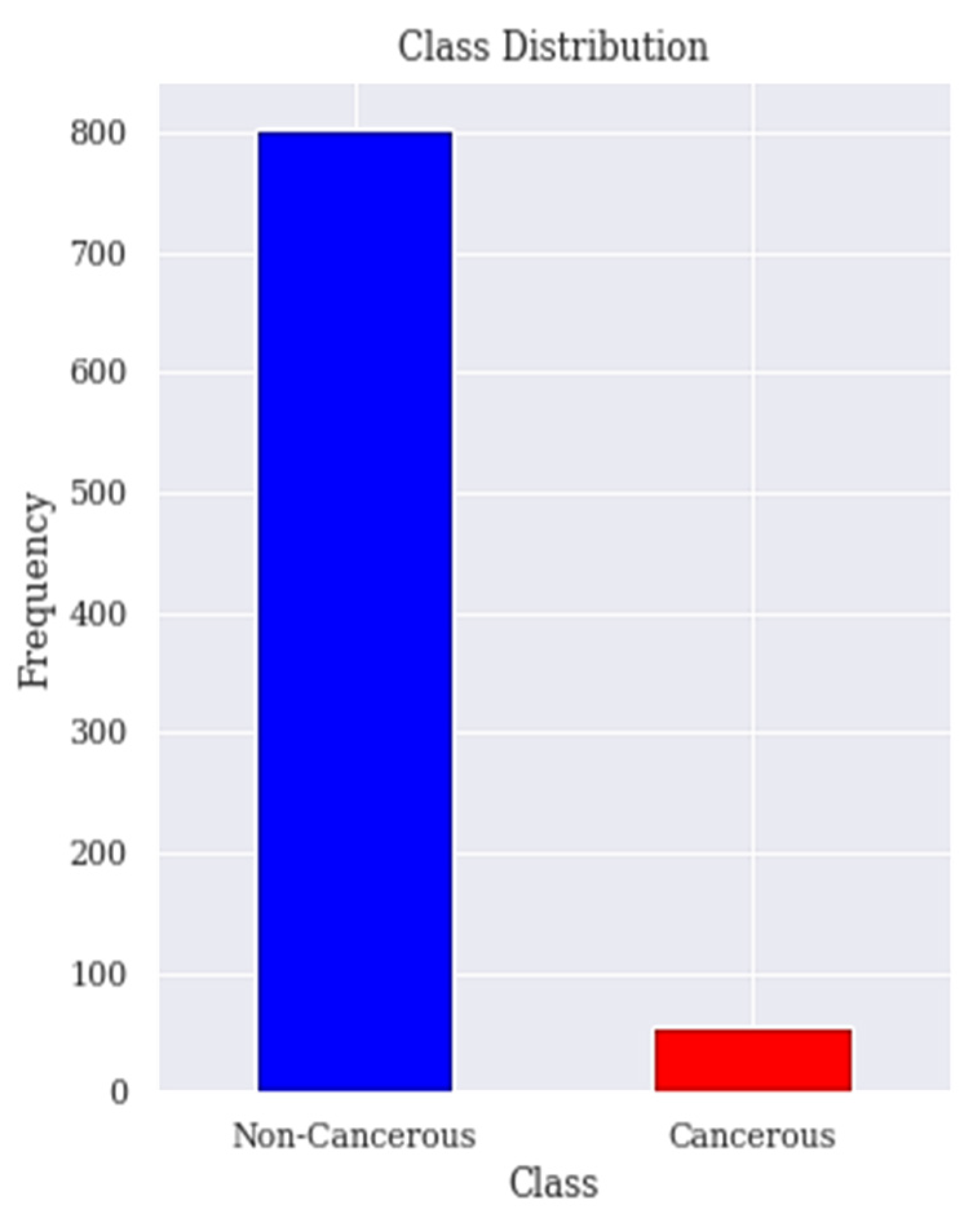
The dataset is collected from the Hospital ‘Universitario de Caracas’ in Caracas, Venezuela. It is published on the UCI (University of California, Irvine) ML repository as Risk Factors dataset [53]. This is a public dataset that contains data of 858 patients (samples) with 36 attributes. The features cover demographic data, habits, and medical records. Unfortunately, the dataset contains missing values accordingly the dataset needs to be treated to deal with the missing values. Those attributes are the risk factors of cervical cancer. The target variables are the diagnosis results of Hinselmann, Schiller, cytology, and biopsy, which are the major diagnosis methods for cervical cancer. In order to ensure the accuracy of our results, the 2 features time since first diagnosis and time since last diagnosis are dropped due to excessive missing values. The biopsy has been the goal standard for diagnosing patients with cervical cancer and our target in this research is to predict the biopsy. Figure 1 shows the class distribution of patient’s with or without cervical cancer in the dataset.
Table 1 shows all the features of the dataset and their corresponding data types, respectively. The features consist of 2 kinds of data types, that is, an integer or a Boolean type. The integer data type represents whole numbers that have no fractional parts while the Boolean data type represents one of two possible values (usually denoted by Yes or No).
3.2. Data Preprocessing
Data pre-processing is applied such that the dataset gets transformed to a state that it can be easily interpreted by our DT model.
The cervical cancer risk factors dataset has a lot of missing values. Therefore, we require an efficient approach for handling such issue. Missing values can either be removed or filled. Removing the missing value approach is best used in large datasets where such removal is insignificant. When we applied the approach to remove the records with missing values the number of rows reduced to 737 from 858. Our aim is to reduce the number of features but not the number of records available in the dataset, hence the strategy of replacing the missing values with mean is used for numerical attributes and mode for categorical attributes and are depicted in Equations (1) and (2), respectively.
where,
xi = ith variable
i = ith value of variable X
n = Number of variables in the dataset
n > 0
where,
L is the lower boundary point of mode class
m represents the mode class
fm−1 is the frequency of the preceding class
fm is the frequency of the mode class
fm+1 is the frequency of the succeeding class
C is the length of the mode class
The features STDs_Time_since_first_diagnosis and STDs_Time_since_last_diagnosis that contained greater than 60% missing values (787 of 858) were also eliminated from the dataset.
3.3. Apply RFE Technique for Feature Selection
The risk factors dataset contains high dimensional data of 33 features after the data cleaning step. Feature selection becomes necessary since some features are less significant to the target variable so their inclusion to the model may lead to:
- Increase in model complexity and makes it difficult to interpret;
- Increase in time complexity for a model to be trained;
- Result in a bloated model with inaccurate predictions.
We applied RFE algorithm to select the optimal subset of features. RFE algorithm firstly fits the DT model to all of the features. Each feature is then ranked according to its importance.
We applied RFE algorithm to select the optimal subset of features. Algorithm 1 gives a description of steps of this procedure. Each feature is ranked according to its importance. Let S be a sequence of ordered numbers representing the number of features to be kept (S1 > S2 > S3…). At each iteration of feature selection algorithm, the Si top ranked features are kept, the model is refit and the accuracy is assessed. The value of Si with the best accuracy is assessed and the top Si features are used to fit the final model. Algorithm 1 gives a description of subsequent steps of this procedure.
| Algorithm 1: Recursive Feature Elimination. |
| Step 1: Train the model using all features Step 2: Determine model’s accuracy Step 3: Determine feature’s importance to the model for each feature Step 4: for each subset Si, i = 1…N do Step 4.1: Keep the Si most important features Step 4.2: Train the model using Si features Step 4.3: Determine model’s accuracy Step 5: end for Step 6: Calculate the accuracy profile over the Si Step 7: Determine the appropriate number of features Step 8: Use the model corresponding to the optimal Si Each feature is ranked according to its importance. |
3.4. Apply LASSO Technique for Feature Selection
LASSO is a linear model that is simple and useful to use. It is defined by the below estimate in Equation (3):
In the above Equation (3), aj is the coefficient of the jth feature. The last term is the L1 penalty and is the hyperparameter that tunes the penalty term.
The higher the coefficient of a feature, the higher the value of the estimated cost function. The rationale behind LASSO technique is to fit the LASSO regression model on our dataset and consider only those features with coefficient greater than 0. The value of is found using cross validation. One major advantage of LASSO is that it performs automatic feature selection. LASSO transforms each and every coefficient by constant component . If there is high correlation in the group of features, LASSO chooses only one among them and shrinks the others to zero. It minimizes the variability of the estimates by shrinking some of the coefficients exactly to zero.
3.5. Resample Class Distribution Using SMOTETomek
The distribution of positive and negative classes of the cervical cancer risk factors dataset is highly imbalanced because 96% of the observations are non-cancerous cases and only 4% are cancerous cases as seen in Figure 1. Previous works have paid little attention to the problem of imbalanced datasets in the cervical cancer risk factors dataset.
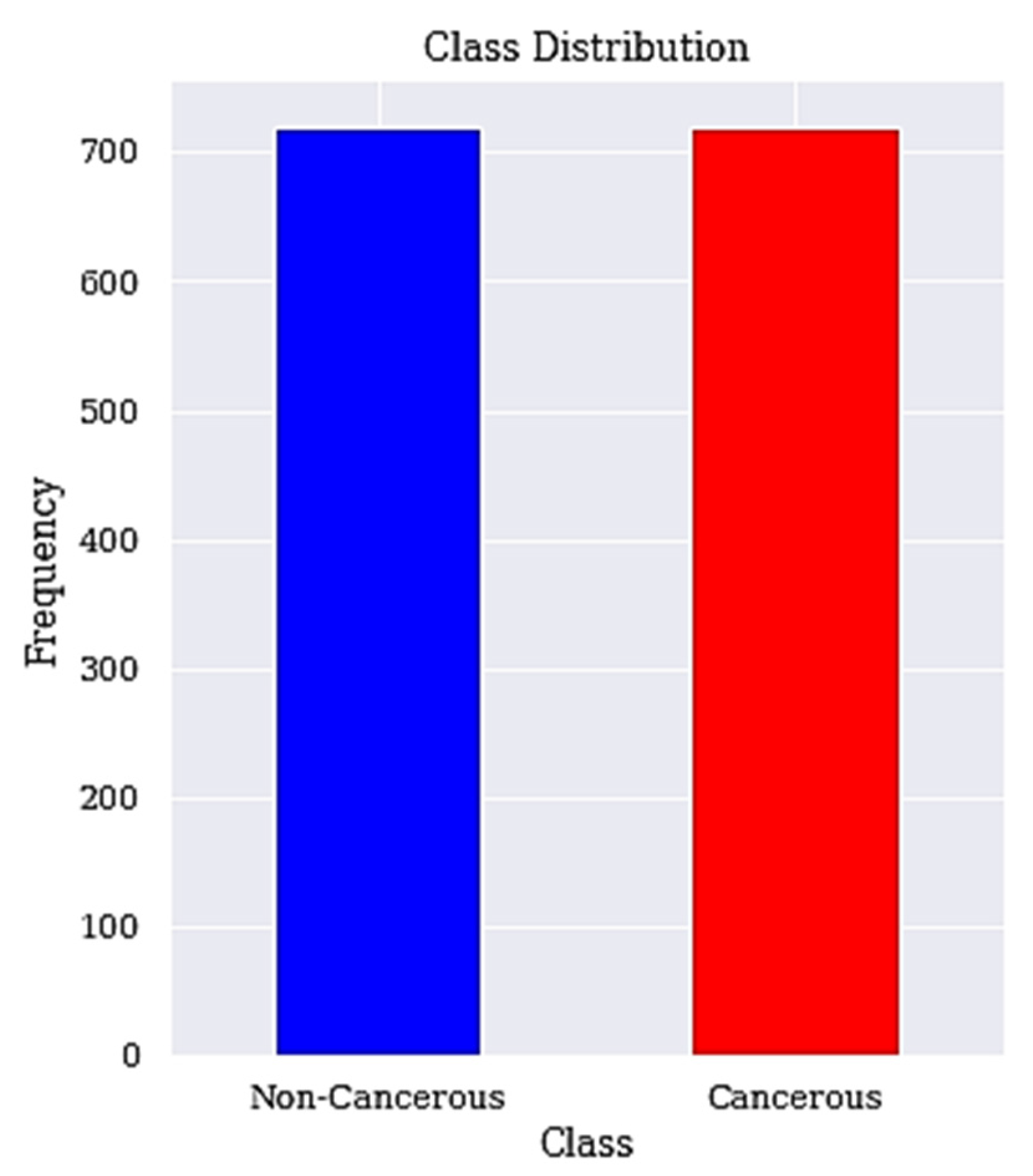
We apply SMOTETomek to balance the high data imbalance in the cervical cancer dataset. The applied resampling technique is SMOTETomek, which combines oversampling (SMOTE) and undersampling (Tomek) and is describe in Algorithm 2 below with the resulting balanced classes described in Figure 2.
| Algorithm 2: SMOTETomek. |
| Step 1: For a dataset D with an unbalanced data distribution, SMOTE is applied to obtain an extended dataset D’ by generating many new minority samples. Step 1.1: Let A be the minority class and let B be the majority class. Step 1.2: for each observation x belongs to class A Step 1.2.1: Identify the K-nearest neighbors of x Step 1.2.2: Randomly select few neighbors Step 1.2.3: Generate artificial observations Step 1.2.4: Spread the observations along the line joining the x to its nearest neighbors. Step 2: Tomek Link pairs in dataset D’ are removed using the Tomek Link method. Step 2.1: Let x be an instance of class A and y an instance of class B. Step 2.2: Let d(x, y) be the distance between x and y. (x, y) is a T-Link Step 2.2.1: if for any instance z, d(x, y) < d(x, z) or d(x, y) < d(y, z) Step 2.3: If any 2 samples are T-Link then one of these samples is a noise or otherwise both samples are located on the boundary of the classes. |
3.6. Classification
The DT with recursive feature elimination (RFE) technique for feature selection and SMOTETomek for data imbalance problem was applied. The choice of DT comes from previous work, where its potential in handing the cervical cancer risk factors dataset has shown to be the most promising when compared to other algorithms [15].
Algorithm 3 defines our general DT model.
| Algorithm 3: DT Learning Algorithm. |
| Step 1: Input Dataset D = {(x1, y1), (x2, y2), ..., (xn, yn)}, Step 1.1: Attribute set A = {a1, a2, ..., am} Step 2: Function (D, A) Step 2.1: create node N Step 2.1.1: if yi = yj(∀yi, yj ∈ D) or xi = xj(∀xi, xj ∈ D) Step 2.1.2: Label (N) = mode(yi) Step 2.1.3: return Step 2.2: end if Step 2.3: choose the optimal partition attribute a* Step 2.4: for every v ∈ value(a*) Step 2.4.1: generate a new branch Dv = {xi|xi(a*) = v} Step 2.4.2: if Dv = ∅ Step 2.4.2.1: Set branch Dv as node Nv Step 2.4.2.2: Label(Nv) = mode(yi), yi ∈ D Step 2.4.3: else Step 2.4.3.1: function(Dv, A − a*) Step 2.4.4: end if Step 2.5: end for Step 3: end |
A grid search (GS) is used to find the optimal parameters for the DT model. The grid search method provides parameters such as the function to measure the quality of split known as the criterion, the maximum depth of tree, the maximum number of features to consider when looking for the best split, the minimum number of samples required to split at each node, and the minimum number of samples required at a leaf node. The optimal values identified by the grid search are: criterion = gini, max_depth = 4, max_features = None, min_samples_leaf = 14, min_samples_splits = 2. It should be noted that by representing our problem in a state-space with limited connectivity we have not changed the underlying intractability of the general model search problem [74]. The idea is to generate a tree with fewer branches that will result in a simpler tree to prevent model overfitting.
3.7. Performance Metrics
In the healthcare sector, the accurate diagnosis of an individual suffering from an ailment is more critical than confirming a person healthy. Therefore, while evaluating a model, accuracy should not be the only metrics to be considered. In this paper, six performance metrics including accuracy, sensitivity, specificity, precision, F-Measure and AUC were used to measure the performance of our model.
The metrics are computed using confusion matrix. A confusion matrix, consist of TP, TN, FP, and FN. It is a table layout that allows visualization of model’s performance. TP represents true positive, where a cancerous person is correctly predicted as having cancer. TN represents true negative, a non-cancerous person correctly predicted as being cancer free. FP connotes false positive, that is, a non-cancerous individual is misclassified as having cancer. FN is short for false negative, delineating a cancerous individual to be free from cancer. It is very clear that that FN is the most important factor that needs to be as small as possible.
These metrics are defined as follows using their basic notations:
- Accuracy: The number of correct predictions by the model out the total number of predictions it is defined in Equation (3).
- 2.
- Sensitivity: The ability of the model to correctly identify people with cervical cancer. A sensitivity of 1 indicates that the model correctly predicted all the people with cervical cancer. It is defined mathematically in Equation (4).
- 3.
- Specificity: This is the metric that evaluates the model’s ability to predict people without cervical cancer. Equation (5) give the definition of specificity.
- 4.
- Precision: This metric measures the proportion of people with cervical cancer and are correctly predicted as having cervical cancer by the model. Precision measures the ratio of people with cervical cancer and are correctly predicted by the model. It is defined mathematically in Equation (6).
- 5.
- F-Measure: It is the combination of precision and sensitivity of the model and is define as the harmonic mean of the model’s precision and sensitivity. A better F-Measure means, we have a smaller number of misclassified people with or without cervical cancer. Equation (7) gives the definition of F-Measure.
- 6.
- Receiving operating characteristics curve (ROC): The ROC is a technique used for visualizing the model’s performance. It is a comprehensive index reflecting the continuous variables of sensitivity and specificity. The curve is used to define the relationship between sensitivity and specificity.
- 7.
- Area under the curve (AUC): The area under the ROC curve, abbreviated as AUC is commonly used to evaluate model’s performance. AUC measures the entire two-dimensional area under the ROC curve. The larger the AUC, the better the performance of the model.
3.8. Computational Framework
This subsection provides more details about the computational framework used in the study. It describes the software and packages used, features of the computer employed, runtimes, and other computational aspects.
The ML model was developed using python programming language. The python code is run on the Google colaboratory known as Google Colab (https://colab.research.google.com/drive/1sY6rW5ThLEtKzTYvvuNzHK6j9IveSXDn?usp=sharing accessed on 22 January 2022). Colab notebooks are Jupyter notebooks that run in the cloud and are highly integrated with Google drive, making them easy to set up, access, and share. The runtime of the application is highly dependent on the speed of the internet. With high internet connectivity, the program can run in less than 23 s. The program is run on Intel Core i5 central processing unit (CPU) with a processing speed of 2.30 GHz. The system has a random-access memory (RAM) of 4 Gigabytes.
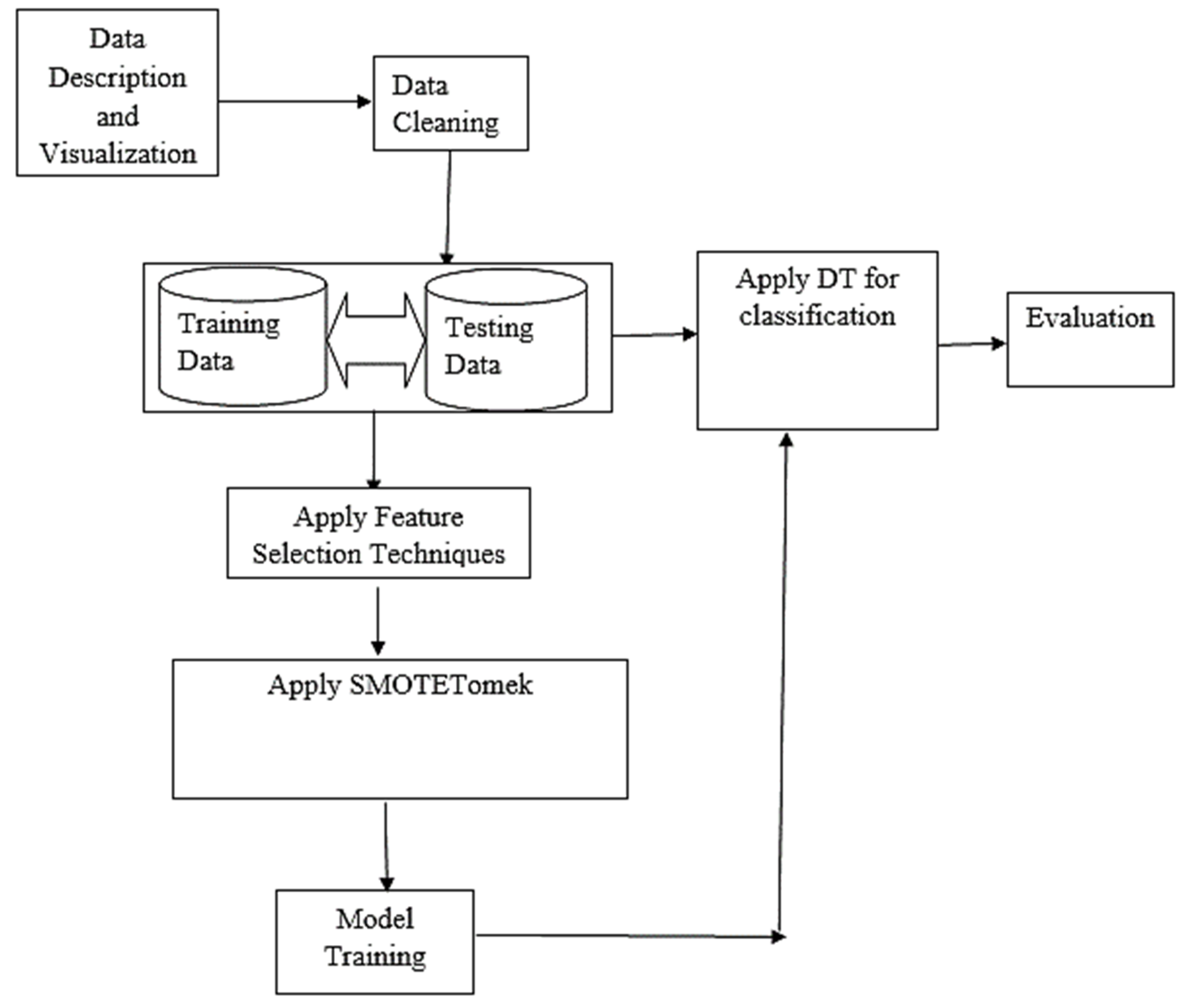
Figure 3 shows the basic architectural framework of the proposed model. It also displayed the organization of model in terms of the various components that make up the system and how they are inter-related.
4. Results and Discussion
This section presents the results obtained for three different classifiers. The performance of the model after series of training and testing on the dataset are presented in a tabular form. We also presented a comprehensive interpretation of the findings of the research and relating them to published works.
While building the DT model, 10-fold cross-validation was applied because observations are limited and may lead to overfitting, which is a drawback of DT algorithm. The estimate of prediction error in 10-fold cross-validation is almost unbiased [78]. Cross-validation method has been recommended for comparing machine learning algorithms when datasets are small since it allows all the data to be involve in both the training and testing [57]. It is a popular approach because it generally results in a less biased estimate of the model skill than other approaches, such as a simple train/test split [58].
4.1. Basic Classification
The first classification task was mainly done to examine the impact of not applying feature selection techniques in predicting cancerous cases. This experiment was therefore conducted without extracting the most relevant features from the dataset. Equations (4)–(8) gives the mathematical representations of the metrics used for experimental evaluation of the DT model. Table 2 provides the breakdown of the first experimental results based on the metrics used in evaluating the model. It shows the result of DT with no feature selection and data balancing techniques applied. These results are the mean scores obtained from 10 folds cross validation.
It has a significant performance in terms of the overall accuracy with an accuracy of 95% and also performed reasonably in predicting patients with negative cervical cancer results with a specificity of 96%. However, the result delivered for true positive cases does not seem promising. The single most striking observation emerge from the results presented in Table 2, is the sensitivity value, which was found to be 86%. The sensitivity is the metric that can best identify positive cases (cancerous cases). Therefore, there is a need to further improve the model, since the research focus on finding patients that are suffering from this ailment.
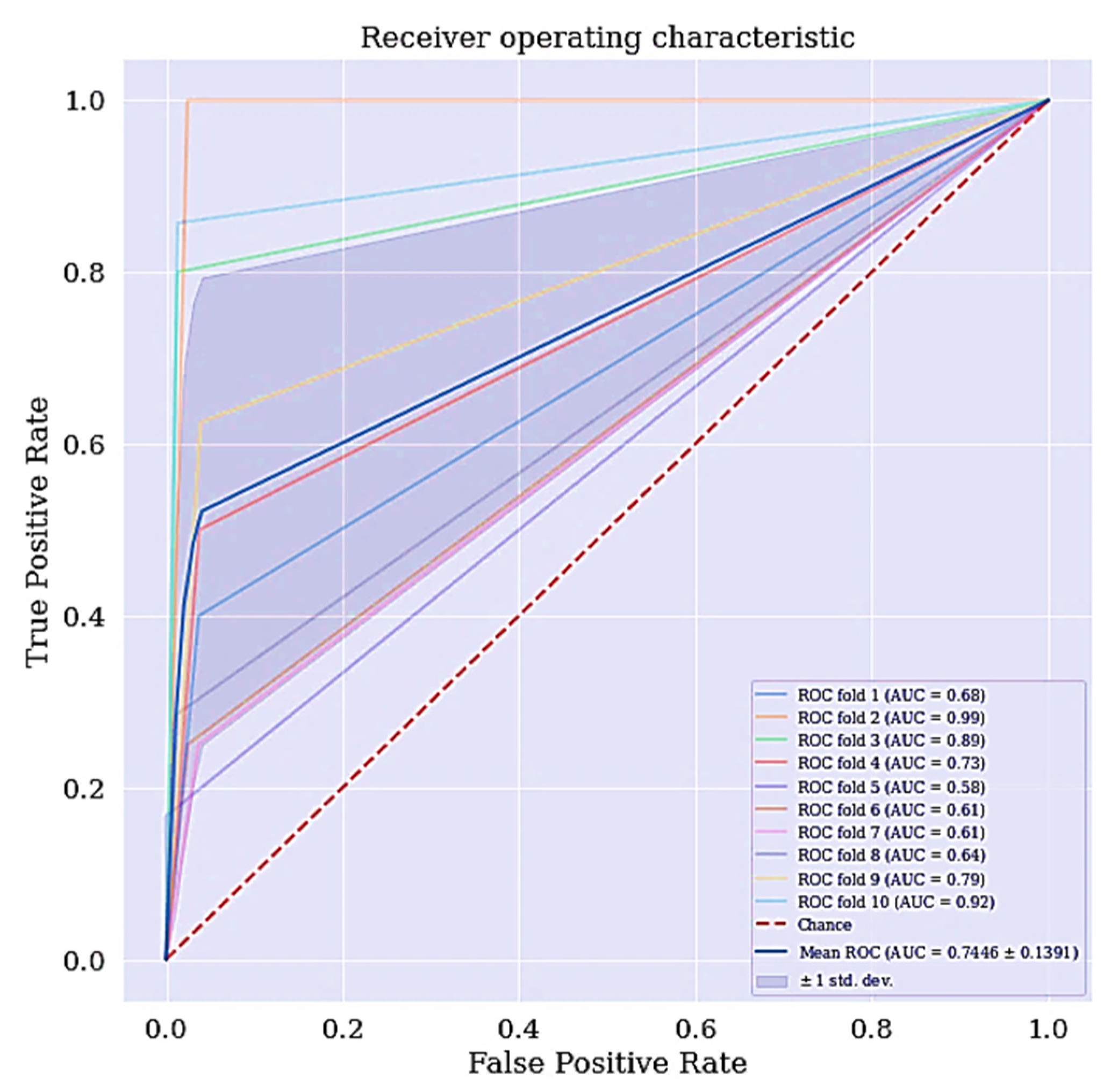
Another metric of interest is precision. While sensitivity expresses the ability of our model to find relevant instances in our data, which is finding the actual people that are suffering from cervical cancer, precision expresses the proportion of those people the model predicted as having cervical cancer but are not suffering from the ailment (false positives). The more false positives we get, the poorer the precision is going to look. Once there is an improvement in the model’s sensitivity and precision, the F-Measure will automatically be improved. F-measure conveys the balance between the precision and sensitivity. The ROC curve for DT classifier is shown in Figure 4. The ROC curve shows the trade-off between sensitivity and specificity. The ROC curve for the DT scenario is a bit centralize. Classifiers that produce curves closer to the top left corner indicate a better performance. Therefore, the ROC curve for the DT classifier can also be improve.
4.2. Improved Classifier with the Selected Features
When we applied the selected features with highest ranking in RFE and the features selected by LASSO. The selected features by RFE as shown in Table 3 are ranked based on their significance in determining whether a patient is cancerous or not while the most relevant features that are selected by LASSO technique with their respective coefficients are shown in Table 4. We obtained a different result as shown in the third and fourth columns of Table 5.
The DT classifier has shown some levels of improvement when the selected features using RFE was applied in terms of the model’s overall accuracy, specificity, precision, f-measure and AUC with an increase of 2.36%, 2.57%, 19.04%, 10.70% and 17.08%, respectively. However, there was no improvement in terms of sensitivity observed. For the selected features from LASSO technique, there is also an improvement in the overall accuracy, specificity, precision, f-measure, and AUC with an increase of 1.18%, 2.56%, 16.66%, 1.91%, and 19.89%, respectively, when compared to DT classifier. Consequently, there is a further need to also improve the current classifiers of both DT + RFE and DT + LASSO.
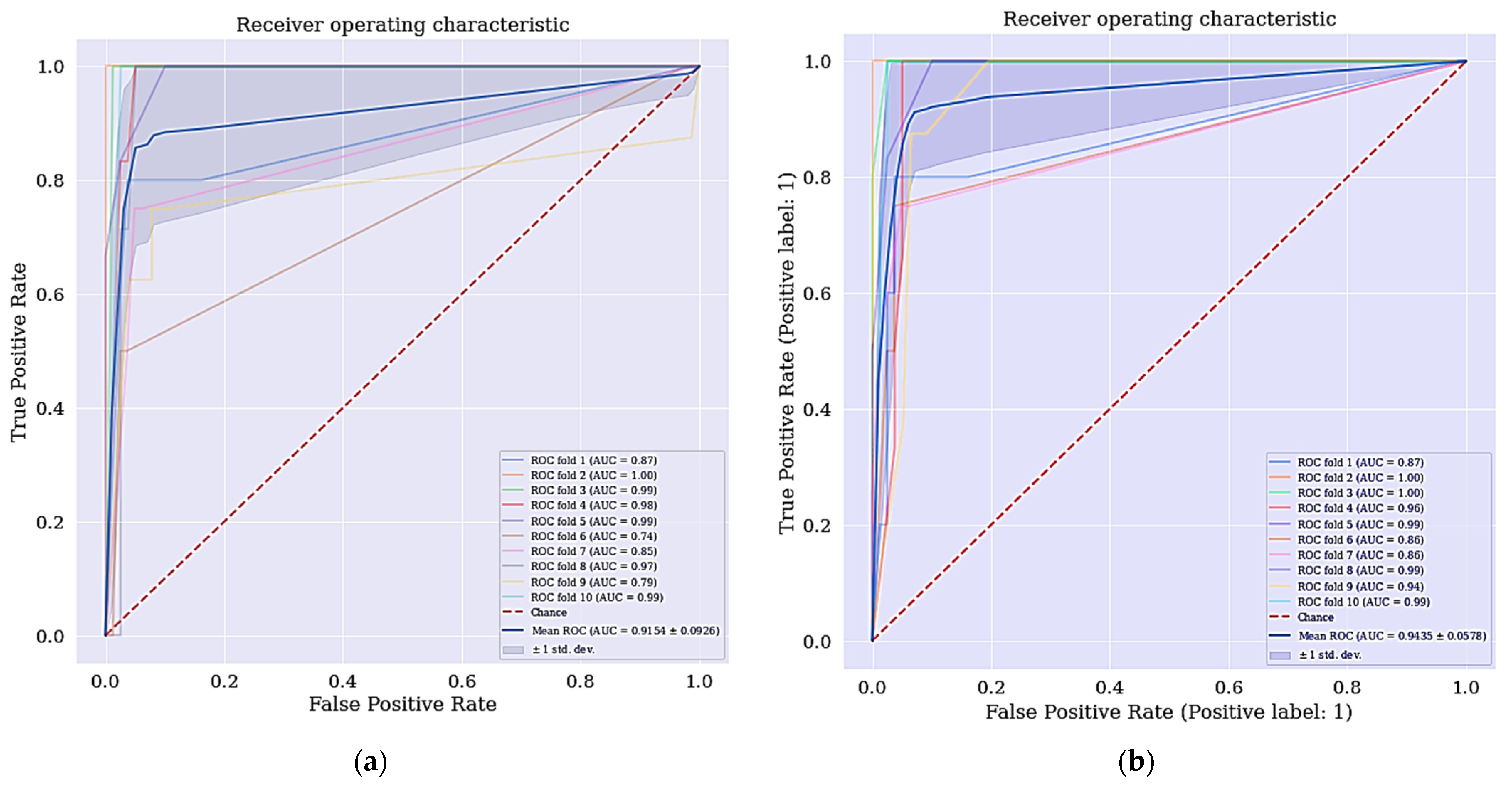
Intriguingly, the cervical cancer risk factors dataset has a problem of imbalanced data where the data collected are not equally represented, we applied a data balancing technique called SMOTETomek. It has some advantages over other techniques, where it undersamples the majority classes and at the same time oversamples the minority classes. Often real-world datasets are predominantly composed of “normal” examples with only a small percentage of “abnormal” or “interesting” examples. This imbalance gives rise to the “class imbalance” problem [37,38,39,40,41,42,43,44,45,46,47,48,49,50,51,52,53,54,55,56,57,58,59,60,61,62,63,64,65,66,67,68,69,70,71,72,73,74,75,76,77,78,79] which is the problem of learning concept from class that has a small number of observations. In the real world, numerous studies have shown that better prediction performance can be achieved by having balanced data; therefore, a number of well-known methods have been developed and used in ML to tackle this issue for improving the prediction models’ performance [80,81]. The ROC curve for DT + RFE and DT + LASSO is shown in Figure 5.
4.3. Improved Classifier with Selected Features and Resample Class Distribution
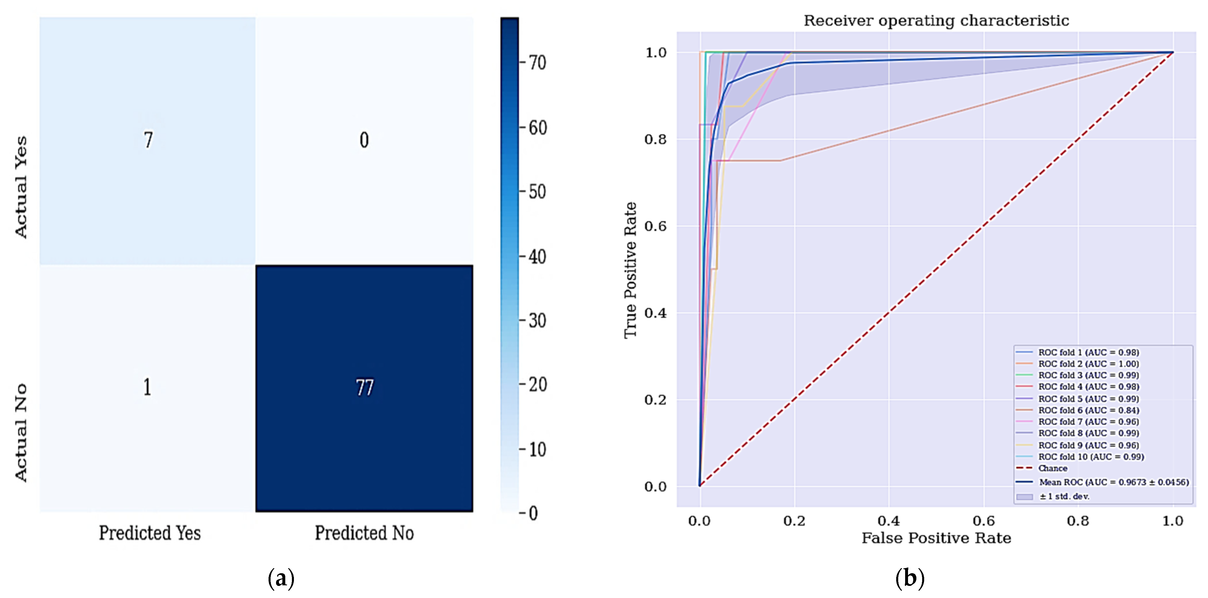
When we applied SMOTETomek as the data balancing technique, we got a different result shown in Table 6. As shown in Table 6, the DT classifier with combination of selected features from RFE and resampled class distribution with SMOTETomek has outperformed the other classifiers in terms of accuracy and sensitivity achieved. The DT + RFE + SMOTETomek yielded an accuracy of 98.82% and sensitivity of 100%, respectively. This is because the work aims to develop a better predictive model that can identify majorly the positive cases.
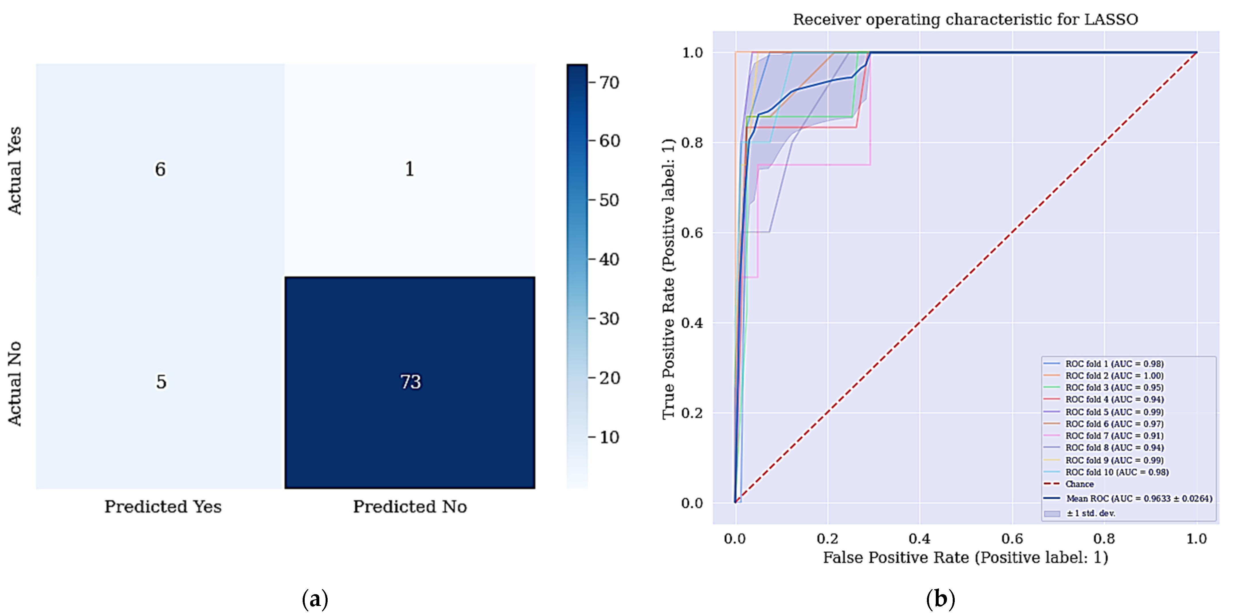
The result in Table 6 revealed that the DT + RFE + SMOTETomek has improved significantly. There was a significant improvement in the accuracy and sensitivity metrics and most interestingly is the sensitivity difference between the models (the difference of 14%). The difference between sensitivities is interesting because it means that the model can best identify positive cases compared to models presented in Section 4.1 and Section 4.2, respectively. Figure 6a shows the confusion matrix for DT + LASSO + SMOTETomek, where a patient who is positive is misclassified as not negative patient. The resulting ROC curve is also shown in Figure 6b.
The aim of this work is achieved since all the positive cases were identified and correctly classified based on the confusion matrix shown in Figure 6. From the data in Figure 7a, it is apparent that no real or actual case was wrongly classified as seen in the confusion matrix. The corresponding ROC curve is shown Figure 7b and has the largest curve with an AUC of approximately 97%.
4.4. Comparison with Previous Studies
We compared the results of our proposed model with past studies that used the cervical cancer risk factors dataset. Table 7 shows the comparison of our results on the basis of accuracy, sensitivity, and specificity for the biopsy test result of our proposed model with Abdoh et al. [59] and Ijaz et al. [68].
The study by Abdoh et al. [59] used SMOTE-RF, SMOTE-RF-RFE, and SMOTE-RF-PCA, while Ijaz et al. [68] used DBSCAN + SMOTETomek + RF, DBSCAN + SMOTE+ RF, iForest + SMOTETomek + RF, and iForest + SMOTE + RF. The four scenarios of our proposed model are RFE + DT, LASSO + DT, RFE + SMOTETomek + DT, and LASSO + SMOTETomek + DT. Our proposed model produces better results as compared to Abdoh et al. [59] and Ijaz et al. [68].
As presented in Table 7, the scenario RFE + SMOTETomek + DT ranks first in terms of accuracy and sensitivity achieved, where we got an accuracy of 98.82% and sensitivity of 100%, respectively. Our RFE + DT also outperformed all the previous studies in terms of the specificity achieved, where we got a specificity of 98.72% but performed below RFE + SMOTETomek + DT in terms of accuracy and sensitivity due to the high class imbalance problem in our dataset, where the negative classes are highly represented.
The work has shown the potential for DT learning for predicting cervical cancer. The DT model is able to handle both numerical and categorical data. This work was able to overcome the problem of overfitting (a problem where decision-tree learners create over-complex trees that do not generalize the data very well) and data imbalance as they are the problems identified from the work of [14]. Mechanisms such as setting the minimum number of samples required at a leaf node and setting the maximum depth of the tree were applied to overcome overfitting. While we applied SMOTETomek, to address the data imbalance problem. Feature selection techniques for dimensionality reduction were applied in our work to fill the gap found in [12]. Finally, the proposed model is relatively improved in terms of the sensitivity when compared to [63].
Taken together, our result shows significant improvement when compared with other approaches. We have described a new process of predicting patients with cervical cancer by selecting the most relevant subset of features through which we achieve better results when compared to previous works. In recent works using the same dataset, the metrics used are accuracy, specificity, sensitivity, precision, f-measure, and AUC. Our model has better sensitivity (metric of interest) over the previously developed models.
5. Conclusions
Cervical cancer is one of the leading causes of premature mortality among women in recent years. According to WHO, more than 85% of cervical cancer cases are mostly reported in developing countries. However, through ML, we are able to recognize the factors that increases possibility of evolving this cancer in women as ranked by RFE. An ML model was implemented to predict the biopsy results of cervical cancer. One of the more significant findings to emerge from this study is that the model using a DT, RFE, and SMOTETomek techniques for feature selection and data resampling has delivered a more reliable predictive model to classify cervical cancer by using patient’s risk factors data. The experimental results indicate significant improvement in the proposed model when compared to other techniques.
The issue of predicting cervical at an early stage can be usefully explored in further research. Further research regarding the role of other feature selection methods such as ridge regression would be worthwhile. It is recommended that further research be undertaken with a very large volume of the dataset so that in-depth analysis and understanding can be performed and a better predictive model can be developed for the same problem. The effect of other hybrid data resampling techniques on the performance of LASSO will be worth exploring.
Future work is intended to be carried out for the long-term management of cervical cancer in clinical and personalized medical management by decision support system.
Author Contributions
Conceptualization, J.J.T. and M.H. (Mohammed Hassan); methodology, J.J.T.; software, J.J.T.; validation, M.H. (Mohamed Hamada), H.K. and J.O.A.; formal analysis, H.K.; investigation, M.H. (Mohamed Hamada); resources, M.H. (Mohamed Hamada); data curation, J.J.T.; writing—original draft preparation, J.J.T.; writing—review and editing, M.H. (Mohamed Hamada), M.H. (Mohammed Hassan) and H.K.; visualization, H.K.; supervision, M.H. (Mohamed Hamada); project administration, J.O.A.; funding acquisition, M.H. (Mohamed Hamada). All authors have read and agreed to the published version of the manuscript.
Funding
This research received no external funding.
Data Availability Statement
The dataset used in this research is publicly available at the UCI machine learning repository on https://archive.ics.uci.edu/ml/datasets/Cervical+cancer+%28Risk+Factors%29 (accessed on 17 July 2021).
Conflicts of Interest
The authors declare no conflict of interest.
References
- WHO. Comprehensive Cervical Cancer Prevention and Control: A Healthier Future for Girls and Women; WHO: Geneva, Switzerland, 2013; pp. 1–12. [Google Scholar]
- Marván, M.L.; López-Vázquez, E. The Anthropocene: Politik–Economics–Society–Science: Preventing Health and Environmental Risks in Latin America; Springer: Berlin/Heidelberg, Germany, 2017. [Google Scholar]
- Ilango, B.; Nithya, V. Evaluation of machine learning based optimized feature selection approaches and classification methods for cervical cancer prediction. SN Appl. Sci. 2019, 1, 641. [Google Scholar]
- IARC. IARC-Incidencia Mundial CM; IARC: Lyon, France, 2018. [Google Scholar]
- Gunnell, A.S. Risk Factors for Cervical Cancer; Universitetsservice US-AB Nanna: Solna, Sweden, 2007. [Google Scholar]
- Castanon, A.; Sasieni, P. Is the recent increase in cervical cancer in women aged 20–24 years in England a cause for concern? Prev. Med. 2018, 107, 21–28. [Google Scholar] [CrossRef] [PubMed]
- Oluwole, E.O.; Mohammed, A.S.; Akinyinka, M.R.; Salako, O. Cervical Cancer Awareness and Screening Uptake among Rural Women in Lagos, Nigeria. J. Community Med. Prim. Health Care 2017, 29, 81–88. [Google Scholar]
- Fernandes, K.; Cardoso, J.; Fernandes, J. Automated Methods for the Decision Support of Cervical Cancer Screening Using Digital Colposcopies. IEEE Access 2018, 6, 33910–33927. [Google Scholar] [CrossRef]
- Jujjavarapu, S.E.; Deshmukh, S. Artificial Neural Network as a Classifier for the Identification of Hepato- cellular Carcinoma Through Prognosticgene Signatures. Curr. Genom. 2018, 19, 483–490. [Google Scholar] [CrossRef]
- Kourou, K.; Exarchos, T.P.; Exarchos, K.P.; Karamouzis, M.V.; Fotiadis, D.I. Machine learning applications in cancer prognosis and prediction. Comput. Struct. Biotechnol. J. 2015, 13, 8–17. [Google Scholar] [CrossRef] [Green Version]
- Singh, H.D.; Cosgrave, N. Diagnosis of Cervical Cancer Using Hybrid Machine Learning Models. Master’s Thesis, National College of Ireland, Dublin, Ireland, 2018. [Google Scholar]
- Fatlawi, H.K. Enhanced Classification Model for Cervical Cancer Dataset based on Cost Sensitive Classifier. Int. J. Comput. Tech. 2017, 4, 115–120. [Google Scholar]
- Alam, T.M.; Milhan, M.; Atif, M.; Wahab, A.; Mushtaq, M. Cervical Cancer Prediction through Different Screening Methods using Data Mining. Int. J. Adv. Comput. Sci. Appl. 2019, 10, 388–396. [Google Scholar] [CrossRef] [Green Version]
- Punjani, D.N.; Atkotiya, K.H. Cervical Cancer Test Identification Classifier using Decision Tree Method. Int. J. Res. Advent Technol. 2019, 7, 169–172. [Google Scholar] [CrossRef]
- Al-Wesabi, Y.M.S.; Choudhury, A.; Won, D. Classification of Cervical Cancer Dataset. In Proceedings of the 2018 IISE Annual Conference, Orlando, FL, USA, 19–22 May 2018; pp. 1456–1461. [Google Scholar]
- Ali, A.; Shaukat, S.; Tayyab, M.; Khan, M.A.; Khan, J.S.; Ahmad, J. Network Intrusion Detection Leveraging Machine Learning and Feature Selection. In Proceedings of the 2020 IEEE 17th International Conference on Smart Communities: Improving Quality of Life Using ICT, IoT and AI (HONET), Charlotte, NC, USA, 14–16 December 2020; pp. 49–53. [Google Scholar]
- Jessica, E.O.; Hamada, M.; Yusuf, S.I.; Hassan, M. The Role of Linear Discriminant Analysis for Accurate Prediction of Breast Cancer. In Proceedings of the 2021 IEEE 14th International Symposium on Embedded Multicore/Many-Core Systems-on-Chip (MCSoC), Singapore, 20–23 December 2021; pp. 340–344. [Google Scholar]
- Alghamdi, M.; Al-Mallah, M.; Keteyian, S.; Brawner, C.; Ehrman, J.; Sakr, S. Predicting diabetes mellitus using SMOTE and ensemble machine learning approach: The Henry Ford ExercIse Testing (FIT) project. PLoS ONE 2017, 12, e0179805. [Google Scholar] [CrossRef]
- Pang-Ning, T.; Steinbach, M.; Kumar, V. Introduction to Data Mining; Pearson Addison-Wesley: Boston, MA, USA, 2006. [Google Scholar]
- Chandrashekar, G.; Sahin, F. A survey on feature selection methods q. Comput. Electr. Eng. 2014, 40, 16–28. [Google Scholar] [CrossRef]
- Alonso-Betanzos, A. Filter Methods for Feature Selection–A Comparative Study; Springer: Berlin/Heidelberg, Germany, 2007. [Google Scholar]
- Peng, Y.; Wu, Z.; Jiang, J. A novel feature selection approach for biomedical data classification. J. Biomed. Inform. 2010, 43, 15–23. [Google Scholar] [CrossRef] [PubMed] [Green Version]
- Chen, X.; Jeong, J.C. Enhanced Recursive Feature Elimination. In Proceedings of the Sixth International Conference on Machine Learning and Applications, Cincinnati, OH, USA, 13–15 December 2007; pp. 429–435. [Google Scholar]
- Go, J.; Łukaszuk, T. Application of The Recursive Feature Elimination And The Relaxed Linear Separability Feature Selection Algorithms To Gene Expression Data Analysis. Adv. Comput. Sci. Res. 2013, 10, 39–52. [Google Scholar]
- Van Ha, S.; Nguyen, H. FRFE: Fast Recursive Feature Elimination for Credit Scoring FRFE: Fast Recursive Feature Elimination. In Proceedings of the International Conference on Nature of Computation and Communication, Rach Gia, Vietnam, 26–18 March 2016; pp. 133–142. [Google Scholar]
- Huang, S.; Cai, N.; Pacheco, P.P.; Narandes, S.; Wang, Y.; Xu, W. Applications of Support Vector Machine (SVM) Learning in Cancer Genomics. Cancer Genom.-Proteom. 2018, 15, 41–51. [Google Scholar]
- Shardlow, M. An Analysis of Feature Selection Techniques; The University of Manchester: Manchester, UK, 2016; pp. 1–7. [Google Scholar]
- Nkiama, H.; Zainudeen, S.; Saidu, M. A Subset Feature Elimination Mechanism for Intrusion Detection System. Int. J. Adv. Comput. Sci. Appl. 2016, 7, 148–157. [Google Scholar] [CrossRef]
- Ahmed, M.; Kabir, M.M.K.; Kabir, M.; Hasan, M.M. Identification of the Risk Factors of Cervical Cancer Applying Feature Selection Approaches. In Proceedings of the 3rd International Conference on Electrical, Computer & Telecommunication Engineering ICECTE 2019, Rajshahi, Bangladesh, 26–28 December 2019; pp. 201–204. [Google Scholar]
- Hamada, M.; Tanimu, J.J.; Hassan, M.; Kakudi, H.A.; Robert, P. Evaluation of Recursive Feature Elimination and LASSO Regularization-based optimized feature selection approaches for cervical cancer prediction. In Proceedings of the 2021 IEEE 14th International Symposium on Embedded Multicore/Many-Core Systems-on-Chip (MCSoC), Singapore, 20–23 December 2021; pp. 333–339. [Google Scholar]
- Rodriguez-galiano, V.F.; Luque-espinar, J.A.; Chica-olmo, M.; Mendes, M.P. Feature selection approaches for predictive modelling of groundwater nitrate pollution: An evaluation of fi lters, embedded and wrapper methods. Sci. Total Environ. 2018, 624, 661–672. [Google Scholar] [CrossRef]
- Tibshirani, R. lasso.pdf. J. R. Stat. Soc. 1996, 58, 267–288. [Google Scholar]
- Yamada, M.; Wittawat, J.; Leonid, S.; Eric, W.P.; Masashi, S. High-Dimensional Feature Selection by Feature-Wise Kernelized Lasso. Neural Comput. 2014, 207, 185–207. [Google Scholar] [CrossRef] [Green Version]
- Ghosh, P.; Azam, S.; Jonkman, M.; Karim, A.; Shamrat, F.M.J.M.; Ignatious, E.; Shultana, S.; Beeravolu, A.R.; De Boer, F. Efficient Prediction of Cardiovascular Disease Using Machine Learning Algorithms With Relief and LASSO Feature Selection Techniques. IEEE Access 2021, 9, 19304–19326. [Google Scholar] [CrossRef]
- Taylor, P.; Ludwig, N.; Feuerriegel, S.; Neumann, D. Journal of Decision Systems Putting Big Data analytics to work: Feature selection for forecasting electricity prices using the LASSO and random forests. J. Decis. Syst. 2015, 2015, 37–41. [Google Scholar]
- Zhang, H.; Wang, J.; Sun, Z.; Zurada, J.M.; Pal, N.R. Feature Selection for Neural Networks Using Group Lasso Regularization. IEEE Trans. Knowl. Data Eng. 2019, 32, 659–673. [Google Scholar] [CrossRef]
- Prati, R.C.; Batista, G.E.A.P.A.; Monard, M.C. Data mining with unbalanced class distributions: Concepts and methods. In Proceedings of the 4th Indian International Conference on Artificial Intelligence, IICAI 2009, Karnataka, India, 16–18 December 2009; pp. 359–376. [Google Scholar]
- Qiang, Y.; Xindong, W. 10 Challenging problems in data mining research. Int. J. Inf. Technol. Decis. Mak. 2006, 5, 597–604. [Google Scholar]
- Rastgoo, M.; Lemaitre, G.; Massich, J.; Morel, O.; Marzani, F.; Garcia, R.; Meriaudeau, F. Tackling the problem of data imbalancing for melanoma classification. In Proceedings of the BIOIMAGING 2016—3rd International Conference on Bioimaging, Proceedings; Part of 9th International Joint Conference on Biomedical Engineering Systems and Technologies, BIOSTEC 2016, Rome, Italy, 21–23 February 2016; pp. 32–39. [Google Scholar]
- Maheshwari, S. A Review on Class Imbalance Problem: Analysis and Potential Solutions. Int. J. Comput. Sci. Issues 2017, 14, 43–51. [Google Scholar]
- Somasundaram, A.; Reddy, U.S. Data Imbalance: Effects and Solutions for Classification of Large and Highly Imbalanced Data. In Proceedings of the 1st International Conference on Research in Engineering, Computers, and Technology (ICRECT 2016), Tiruchirappalli, India, 8–10 September 2016; pp. 28–34. [Google Scholar]
- Cengiz Colak, M.; Karaaslan, E.; Colak, C.; Arslan, A.K.; Erdil, N. Handling imbalanced class problem for the prediction of atrial fibrillation in obese patient. Biomed. Res. 2017, 28, 3293–3299. [Google Scholar]
- Yan, Y.; Liu, R.; Ding, Z.; Du, X.; Chen, J.; Zhang, Y. A parameter-free cleaning method for SMOTE in imbalanced classification. IEEE Access 2019, 7, 23537–23548. [Google Scholar] [CrossRef]
- Wang, Z.H.E.; Wu, C.; Zheng, K.; Niu, X.; Wang, X. SMOTETomek-based Resampling for Personality Recognition. IEEE Access 2019, 7, 129678–129689. [Google Scholar] [CrossRef]
- More, A. Survey of resampling techniques for improving classification performance in unbalanced datasets. arXiv 2016, arXiv:1608.06048. [Google Scholar]
- Goel, G.; Maguire, L.; Li, Y.; McLoone, S. Evaluation of Sampling Methods for Learning from Imbalanced Data. In Intelligent Computing Theories; Springer: Berlin/Heidelberg, Germany, 2013; pp. 392–401. [Google Scholar]
- Chen, T.; Shi, X.; Wong, Y.D. Key feature selection and risk prediction for lane-changing behaviors based on vehicles’ trajectory data. Accid. Anal. Prev. 2019, 129, 156–169. [Google Scholar] [CrossRef]
- Le, T.; Baik, S.W. A Robust Framework for Self-Care Problem Identification for Children with Disability. Symmetry 2019, 11, 89. [Google Scholar] [CrossRef] [Green Version]
- Teixeira, V.; Camacho, R.; Ferreira, P.G. Learning influential genes on cancer gene expression data with stacked denoising autoencoders. In Proceedings of the 2017 IEEE International Conference on Bioinformatics and Biomedicine (BIBM), Kansas City, MO, USA, 23–16 November 2017; pp. 1201–1205. [Google Scholar]
- Fitriyani, N.L.; Syafrudin, M.; Alfian, G.; Rhee, J. Development of Disease Prediction Model Based on Ensemble Learning Approach for Diabetes and Hypertension. IEEE Access 2019, 7, 144777–144789. [Google Scholar] [CrossRef]
- Zeng, M.; Zou, B.; Wei, F.; Liu, X.; Wang, L. Effective prediction of threecommondiseases by combining SMOTE with Tomek links technique for imbalanced medical data. In Proceedings of the 2016 IEEE International Conference of Online Analysis and Computing Science (ICOACS), Chongqing, China, 28–29 May 2016; pp. 225–228. [Google Scholar]
- William, W.; Ware, A.; Basaza-ejiri, A.H.; Obungoloch, J. A review of image analysis and machine learning techniques for automated cervical cancer screening from pap-smear images. Comput. Methods Programs Biomed. 2018, 164, 15–22. [Google Scholar] [CrossRef]
- Fernandes, K.; Cardoso, J.S.; Fernandes, J. Transfer learning with partial observability applied to cervical cancer screening. In Proceedings of the Iberian Conference on Pattern Recognition and Image Analysis, Faro, Portugal, 20–23 June 2017; Springer: Cham, Switzerland, 2017; pp. 243–250. [Google Scholar]
- Wu, W.; Zhou, H. Data-Driven Diagnosis of Cervical Cancer With Support Vector Machine-Based Approaches. IEEE Access 2017, 5, 25189–25195. [Google Scholar] [CrossRef]
- Shah, J.H.; Sharif, M.; Yasmin, M.; Fernandes, S.L. Facial expressions classification and false label reduction using LDA and threefold SVM. Pattern Recognit. Lett. 2017, 139, 166–173. [Google Scholar] [CrossRef]
- Karamizadeh, S.; Abdullah, S.M.; Halimi, M.; Shayan, J.; Rajabi, M.J. Advantage and drawback of support vector machine functionality. In Proceedings of the I4CT 2014-1st International Conference on Computer, Communications, and Control Technology, Kedah, Malaysia, 2–4 September 2014; pp. 63–65. [Google Scholar]
- Raschka, S. Model Evaluation, Model Selection, and Algorithm Selection in Machine Learning. arXiv 2020, arXiv:1811.12808. [Google Scholar]
- Yadav, S. Analysis of k-fold cross-validation over hold-out validation on colossal datasets for quality classification. In Proceedings of the 2016 IEEE 6th International Conference on Advanced Computing (IACC), Bhimavaram, India, 27–28 February 2016. [Google Scholar]
- Abdoh, S.F.; Rizka, M.A.; Maghraby, F.A. Cervical Cancer Diagnosis Using Random Forest Classifier With SMOTE and Feature Reduction Techniques. IEEE Access 2018, 6, 59475–59485. [Google Scholar] [CrossRef]
- Deng, X.; Luo, T.; Wang, C. Analysis of Risk Factors for Cervical Cancer Based on Machine Learning Methods. In Proceedings of the 2018 5th IEEE International Conference on Cloud Computing and Intelligence Systems (CCIS), Nanjing, China, 23–25 November 2018; pp. 631–635. [Google Scholar]
- Alsmariy, R.; Healy, G.; Abdelhafez, H. Predicting Cervical Cancer using Machine Learning Methods. Int. J. Adv. Comput. Sci. Appl. 2020, 11, 173–184. [Google Scholar] [CrossRef]
- Ghoneim, A.; Muhammad, G.; Hossain, S.M. Machine learning for assisting cervical cancer diagnosis: An ensemble approach, Futur. Gener. Comput. Syst. 2020, 106, 199–205. [Google Scholar]
- Ghoneim, A.; Muhammad, G.; Hossain, M.S. Cervical cancer classification using convolutional neural networks and extreme learning machines. Future Gener. Comput. Syst. 2019, 102, 643–649. [Google Scholar] [CrossRef]
- Musa, A.; Hamada, M.; Aliyu, F.M.; Hassan, M. An Intelligent Plant Dissease Detection System for Smart Hydroponic using Convolutional Neural Network. In Proceedings of the 2021 IEEE 14th International Symposium on Embedded Multicore/Many-Core Systems-on-Chip (MCSoC), Singapore, 20–23 December 2021; pp. 345–351. [Google Scholar]
- Sepandi, M.; Taghdir, M.; Rezaianzadeh, A.; Rahimikazerooni, S. Assessing Breast Cancer Risk with an Artificial Neural Network. Asian Pac. J. Cancer Prev. 2018, 19, 1017–1019. [Google Scholar]
- Ayer, T.; Alagoz, O.; Chhatwal, J.; Shavlik, J.W.; Kahn, C.; Burnside, E.S. Breast cancer risk estimation with artificial neural networks revisited. Cancer 2010, 116, 3310–3321. [Google Scholar] [CrossRef] [Green Version]
- Yamashita, R.; Nishio, M.; Do, R.K.G.; Togashi, K. Convolutional neural networks: An overview and application in radiology. Insights Imaging 2018, 9, 611–629. [Google Scholar] [CrossRef] [Green Version]
- Ijaz, M.F.; Attique, M.; Son, Y. Data-Driven Cervical Cancer Prediction Model with Outlier Detection and Over-Sampling Methods. Sensors 2020, 20, 2809. [Google Scholar] [CrossRef]
- Saxena, R. Building Decision Tree Algorithm in Python with Decision Tree Algorithm Implementation with Scikit Learn How We Can Implement Decision Tree Classifier. 2018, pp. 1–16. Available online: https://dataaspirant.com/decision-tree-algorithm-python-with-scikit-learn/ (accessed on 1 February 2017).
- Jujjavarapu, S.; Chandrakar, N. Artificial neural networks as classification and diagnostic tools for lymph node-negative breast cancers. Korean J. Chem. Eng. 2016, 33, 1318–1324. [Google Scholar]
- De Ville, B. Decision Trees for Business Intelligence and Data Mining: Using SAS Enterprise Miner. Lect. Notes Math. 2008, 1928, 67–86. [Google Scholar]
- Shekar, B.H.; Dagnew, G. Grid Search-Based Hyperparameter Tuning and Classification of Microarray Cancer Data. In Proceedings of the Second International Conference on Advanced Computational and Communication Paradigms (ICACCP-2019), Gangtok, India, 25–28 February 2019. [Google Scholar]
- Tabares-Soto, R.; Orozco-Arias, S.; Romero-Cano, V.; Bucheli, V.S.; Rodríguez-Sotelo, J.L.; Jiménez-Varón, C.F. A comparative study of machine learning and deep learning algorithms to classify cancer types based on microarray gene expression data. PeerJ Comput. Sci. 2020, 6, e270. [Google Scholar] [CrossRef] [PubMed] [Green Version]
- Bramer, M. Principles of Data Mining; Springer: Berlin/Heidelberg, Germany, 2007. [Google Scholar]
- Kerdprasop, N. Discrete Decision Tree Induction to Avoid Overfitting on Categorical Data. In Proceedings of the MAMECTIS/NOLASC/CONTROL/WAMUS’11, Iasi, Romania, 1–3 July 2011. [Google Scholar]
- Patel, R.; Aluvalu, R. A Reduced Error Pruning Technique for Improving Accuracy of Decision Tree Learning. Int. J. Adv. Sci. Eng. Inf. Technol. 2014, 3, 8–11. [Google Scholar]
- Patil, D.D.; Wadhai, V.; Gokhale, J. Evaluation of Decision Tree Pruning Algorithms for Complexity and Classification Accuracy. Int. J. Comput. Appl. 2010, 11, 23–30. [Google Scholar] [CrossRef]
- Berrar, D. Cross-Validation. In Reference Module in Life Sciences; Elsevier: Amsterdam, The Netherlands, 2019. [Google Scholar]
- Hassan, M. Smart Media-based Context-aware Recommender Systems for Learning: A Conceptual Framework. In Proceedings of the 16th International Conference on Information Technology Based Higher Education and Training (ITHET), Ohrid, Macedonia, 10–12 June 2017. [Google Scholar]
- Hassan, M. A Fuzzy-based Approach for Modelling Preferences of Users in Multi-criteria Recommender Systems. In Proceedings of the 2018 IEEE 12th International Symposium on Embedded Multicore/Many-Core Systems-on-Chip (MCSoC), Hanoi, Vietnam, 12–14 September 2018. [Google Scholar]
- Tanimu, J.J.; Hamada, M.; Hassan, M.; Yusuf, S.I. A Contemporary Machine Learning Method for Accurate Prediction of Cervical Cancer. In Proceedings of the 3rd ETLTC2021-ACM International Conference om Information and Communications Technology, Aizu, Japan, 27–30 January 2021; p. 04004. [Google Scholar]
Figure 1.
Class distribution. The class distribution of people with and without cervical cancer in the dataset is shown here.
Figure 1.
Class distribution. The class distribution of people with and without cervical cancer in the dataset is shown here.

Figure 2.
Balanced class distribution. The class distribution after resampling is shown here.

Figure 3.
Architecture of the model.

Figure 4.
ROC curve for DT without RFE and SMOTETomek.

Figure 5.
(a) ROC curve for DT + RFE; (b) ROC curve for DT + LASSO.

Figure 6.
(a) Confusion matrix for DT + LASSO + SMOTETomek and (b) ROC Curve for DT + LASSO + SMOTETomek techniques. (a) shows the confusion matrix of DT + LASSO + SMOTETomek and its resulting AUC.
Figure 6.
(a) Confusion matrix for DT + LASSO + SMOTETomek and (b) ROC Curve for DT + LASSO + SMOTETomek techniques. (a) shows the confusion matrix of DT + LASSO + SMOTETomek and its resulting AUC.

Figure 7.
(a) Confusion matrix for DT + RFE + SMOTETomek and (b) ROC Curve for DT + RFE + SMOTETomek techniques. Figure 6a shows the confusion matrix of DT + RFE + SMOTETomek and its resulting AUC.
Figure 7.
(a) Confusion matrix for DT + RFE + SMOTETomek and (b) ROC Curve for DT + RFE + SMOTETomek techniques. Figure 6a shows the confusion matrix of DT + RFE + SMOTETomek and its resulting AUC.


Table 1.
Characteristics of Dataset.
| S/N | Features | Data Types |
|---|---|---|
| 1 | Age | Integer |
| 2 | Number of sexual partners | Integer |
| 3 | First sexual intercourse (age) | Integer |
| 4 | Number of pregnancies | Integer |
| 5 | Smokes | Boolean |
| 6 | Smokes (years) | Integer |
| 7 | Smokes (packs/year) | Integer |
| 8 | Hormonal contraceptives | Boolean |
| 9 | Hormonal contraceptives (years) | Integer |
| 10 | IUD | Boolean |
| 11 | IUD (years) | Integer |
| 12 | STDs | Boolean |
| 13 | STDs (number) | Integer |
| 14 | STDS: Condylomatosis | Boolean |
| 15 | STDS: Cervical condylomatosis | Boolean |
| 16 | STDS: Cervical condylomatosis | Boolean |
| 17 | STDS: Vulvo-perineal condylomatosis | Boolean |
| 18 | STDS: Syphilis | Boolean |
| 19 | STDS: Pelvic inflammatory disease | Boolean |
| 20 | STDS: Genital herpes | Boolean |
| 21 | STDS: Molluscum cotagiosum | Boolean |
| 22 | STDS: AIDS | Boolean |
| 23 | STDS: HIV | Boolean |
| 24 | STDS: Hepatits B | Boolean |
| 25 | STDS: HPV | Boolean |
| 26 | STDS: Number of diagnoses | Integer |
| 27 | STDS: Time since first diagnosis | Integer |
| 28 | STDS: Time since last diagnosis | Integer |
| 29 | Dx: Cancer | Boolean |
| 30 | Dx: CIN | Boolean |
| 31 | Dx: HPV | Boolean |
| 32 | Dx: | Boolean |
| 33 | Hinselmann | Boolean |
| 34 | Schiller | Boolean |
| 35 | Cytology | Boolean |
| 36 | Biopsy (Target) | Boolean |
Table 2.
Results of DT without applying RFE and SMOTETomek techniques.
| Evaluation Metrics | DT Performance |
|---|---|
| Accuracy | 95.29% |
| Sensitivity | 85.71% |
| Specificity | 96.15% |
| Precision | 66.67% |
| F-measure | 75.01% |
| AUC | 74.46% |
Table 3.
Top ranked features in RFE.
| SN | Features |
|---|---|
| 1 | Age |
| 2 | Dx: |
| 3 | Dx: CIN |
| 4 | Dx: Cancer |
| 5 | STDs: Number of diagnoses |
| 6 | STDs: HPV |
| 7 | STDs: Hepatitis B |
| 8 | STDs: HIV |
| 9 | STDs: AIDS |
| 10 | STDs: Molluscum contagiosum |
| 11 | Hormonal contraceptives (years) |
| 12 | Number of sexual partners |
| 13 | First sexual intercourse |
| 14 | STDs |
| 15 | IUD (years) |
| 16 | IUD |
| 17 | Hormonal contraceptives |
| 18 | Smokes (packs/year) |
| 19 | Smokes |
| 20 | Number of pregnancies |
Table 4.
Features selected by LASSO with their estimated coefficients.
| Features | LASSO Coefficients |
|---|---|
| Age | −2.912 |
| Number of sexual partners | −4.133 |
| First sexual intercourse (age) | −6.216 |
| Smokes (years) | −2.697 |
| Smokes (packs/year) | 1.858 |
| Hormonal contraceptives (years) | 5.706 |
| STDs | 1.802 |
| STDS: Syphilis | −8.344 |
| Dx: CIN | 2.473 |
| Dx: | 2.875 |
Table 5.
Results of DT with the selected features.
| Evaluation Metrics | DT | DT + RFE | DT + LASSO |
|---|---|---|---|
| Accuracy | 95.29% | 97.65% | 96.47% |
| Sensitivity | 85.71% | 85.71% | 71.43% |
| Specificity | 96.15% | 98.72% | 98.71% |
| Precision | 66.67% | 85.71% | 83.33% |
| F-Measure | 75.01% | 85.71% | 76.92% |
| AUC | 74.46% | 91.54% | 94.35% |
Table 6.
Results of DT with selected features and balanced classes.
| Evaluation Metrics | DT + RFE + SMOTETomek | DT + LASSO + SMOTETomek |
|---|---|---|
| Accuracy | 98.82% | 92.94% |
| Sensitivity | 100% | 85.71% |
| Specificity | 98.71% | 93.59% |
| Precision | 87.51% | 54.55% |
| F-Measure | 93.33% | 66.67% |
| AUC | 96.73% | 96.33% |
Table 7.
Comparison of biopsy test results of our model with past studies.
| Studies | Method | No. of Features | Accuracy | Sensitivity | Specificity |
|---|---|---|---|---|---|
| Abdoh et al. [59] | SMOTE-RF | 30 | 96.06% | 94.55% | 97.51% |
| SMOTE-RF-RFE | 18 | 95.87% | 94.42% | 97.26% | |
| SMOTE-RF-PCA | 11 | 95.74% | 94.16% | 97.76% | |
| Ijaz et al. [68] | DBSCAN + SMOTETomek + RF | 10 | 97.72% | 97.43% | 98.01% |
| DBSCAN + SMOTE+ RF | 10 | 97.22% | 96.43% | 98.01% | |
| iForest + SMOTETomek + RF | 10 | 97.50% | 97.91% | 97.08% | |
| iForest + SMOTE + RF | 10 | 97.58% | 97.45% | 97.58% | |
| Present Studies | RFE + DT | 20 | 97.65% | 85.71% | 98.72% |
| LASSO + DT | 10 | 96.47% | 71.43% | 98.71% | |
| RFE + SMOTETomek + DT | 20 | 98.82% | 100% | 98.71% | |
| LASSO + SMOTETomek + DT | 10 | 92.94% | 85.71% | 93.59% |
Publisher’s Note: MDPI stays neutral with regard to jurisdictional claims in published maps and institutional affiliations. |
© 2022 by the authors. Licensee MDPI, Basel, Switzerland. This article is an open access article distributed under the terms and conditions of the Creative Commons Attribution (CC BY) license (https://creativecommons.org/licenses/by/4.0/).
Share and Cite
MDPI and ACS Style
Tanimu, J.J.; Hamada, M.; Hassan, M.; Kakudi, H.; Abiodun, J.O. A Machine Learning Method for Classification of Cervical Cancer. Electronics 2022, 11, 463. https://doi.org/10.3390/electronics11030463
AMA Style
Tanimu JJ, Hamada M, Hassan M, Kakudi H, Abiodun JO. A Machine Learning Method for Classification of Cervical Cancer. Electronics. 2022; 11(3):463. https://doi.org/10.3390/electronics11030463
Chicago/Turabian StyleTanimu, Jesse Jeremiah, Mohamed Hamada, Mohammed Hassan, Habeebah Kakudi, and John Oladunjoye Abiodun. 2022. "A Machine Learning Method for Classification of Cervical Cancer" Electronics 11, no. 3: 463. https://doi.org/10.3390/electronics11030463
Note that from the first issue of 2016, this journal uses article numbers instead of page numbers. See further details here.