Article

Theoretical Study of the Input Impedance and Electromagnetic Field Distribution of a Dipole Antenna Printed on an Electrical/Magnetic Uniaxial Anisotropic Substrate

by
Mohamed Lamine Bouknia
1,
Chemseddine Zebiri
1,
Djamel Sayad
2,
Issa Elfergani
3,4,*,
Jonathan Rodriguez
3,5,
Mohammad Alibakhshikenari
6,*,
Raed A. Abd-Alhameed
4,
Francisco Falcone
7 and
Ernesto Limiti
6
1
Laboratoire d’Electronique de Puissance et Commande Industrielle (LEPCI), Department of Electronics, University of Ferhat Abbas, Sétif -1-, Sétif 19000, Algeria
2
Laboratoire d’Electrotechnique de Skikda (LES), University 20 Aout 1955-Skikda, Skikda 21000, Algeria
3
Instituto de Telecomunicações, Campus Universitário de Santiago, 3810-193 Aveiro, Portugal
4
School of Electrical Engineering and Computer Science, University of Bradford, Bradford BD71DP, UK
5
Faculty of Computing, Engineering and Science, University of South Wales, Pontypridd CF37 1DL, UK
6
Electronic Engineering Department, University of Rome “Tor Vergata”, Via Del Politecnico 1, 00133 Rome, Italy
7
Electric, Electronic and Communication Engineering Department, Public University of Navarre, 31006 Pamplona, Spain
*
Authors to whom correspondence should be addressed.
Electronics 2021, 10(9), 1050; https://doi.org/10.3390/electronics10091050
Submission received: 31 March 2021 / Revised: 24 April 2021 / Accepted: 26 April 2021 / Published: 29 April 2021
(This article belongs to the Special Issue Recent Advances in Antenna Design for 5G Heterogeneous Networks)

Abstract

:
The present work considers the investigation of the effects of both electrical and magnetic uniaxial anisotropies on the input impedance, resonant length, and fields distribution of a dipole printed on an anisotropic grounded substrate. In this study, the associated integral equation, based on the derivation of the Green’s functions in the spectral domain, is numerically solved employing the method of moments. In order to validate the computing method and the evaluated calculation code, numerical results are compared with available data in the literature treating particular cases of electrical uniaxial anisotropy; reasonable agreements are reported. Novel results of the magnetic uniaxial anisotropy effects on the input impedance and the evaluated electromagnetic field are presented and discussed. This work will serve as a stepping stone for further works for a better understanding of the electromagnetic field behavior in complex anisotropic and bi-anisotropic media.

1. Introduction

Since a few decades, theoretical and experimental studies of the interaction of electromagnetic waves with complex-media structures, anisotropic or bianisotropic, have been extensively investigated for their innovative applications, including geophysical explorations, communications with buried and submerged antennas, microwave/millimeter integrated circuits, optical devices, etc. [1,2,3,4,5,6,7].
In general, complex media have received increasing interest from both scientists and researchers in the context of artificial media with new and interesting properties due to their additional degree of freedom [8]. Anisotropy is an intrinsic property found in crystals, layered structures, composite materials, and other natural materials, in addition to artificial materials. The effect of anisotropy must be considered and cannot be ignored in the prediction of unusual properties in engineering designs such as for sensing and antenna applications [9,10,11]. They have attracted much interest and support from researchers and manufacturers as powerful instruments with interesting growth potential in microwave applications [12]. Many studies have been performed to characterize microwave structures printed on complex media, ferrites, metamaterials, chiral by employing numerical and analytical methods [11,12,13,14,15,16,17,18,19,20,21,22,23,24]. In [11], a detailed analytical model is derived for the circularly polarized slot antenna, built on a ferrite substrate. This model is based on an integral equation for the radial electric field on the slot. In [12], a patch antenna model is first simulated using the finite element method-based HFSS software and then fabricated on a multiple-ferrite-cored substrate. Recently, in [13], Karma et al. studied microstrip transmission lines with anisotropic and uniaxial anisotropic substrates using the discrete mode matching method. A technique for the calculation of the input impedance of a microstrip antenna printed on chiral substrate based on the integral equation with the Cauchy singularity is derived in [14]. This technique is used in [15] to investigate the dependences of the input impedance, the magnitude and phase of the electric-field components on the radiator length for different types of chiral substrates. In [16], a method based on the volume integral equation (VIE) is used to evaluate the electromagnetic (EM) fields scattered by general anisotropic multilayer structures. In [17,18], for a microstrip patch antenna, the effect of a bianisotropic gyro-chiral substrate on the complex resonant frequency, half-power bandwidth and input impedance, and on the surface waves is presented, respectively. The analysis is based on the full-wave spectral method of moments using sinusoidal basis functions. In [19], the far field radiation of a Hertzian dipole for two-layered uniaxial anisotropic medium is investigated using the spectral method of moments based on the derivation of the spectral dyadic Green’s functions (DGFs) to examine the effect of anisotropy, effect of layer thickness, and effect of dipole location on the radiation fields. The effect of the dielectric constitutive parameters on the input impedance and resonance lengths of a dipole antenna based on stratified electrical anisotropic and chiral substrates and a microstrip patch have been analyzed in [20,21,22,23] using the spectral method of moments [24]. Many attempts have been made to analyze the problem of dipole antennas on an anisotropic uniaxial media with the optical axis perpendicular to the substrate plane [25,26,27,28,29] and with arbitrary optical axes orientations [30]. The input impedance and mutual coupling of single and multilayer dipole antennas printed on isotropic, anisotropic, and chiral materials have been studied in [29,31,32,33,34].
This work extends past research works on printed dipoles by studying a planar dipole of arbitrary length printed on a uniaxial anisotropic dielectric structure. The electromagnetic field distributions and input impedance are examined by applying the spectral method of moments based on the immittance functions derivation [35,36,37,38]. The Method of Moments in the spectral domain is found to be a powerful numerical technique to solve integral equations [39], and considered as rigorous and full-wave numerical technique for solving open boundary electromagnetic problems and the employing of this method becomes an increasingly important research issue [4,5,6,7,8,9,10,17,18,19,20,21,22,23,24,28,29,30,31,34,35,36,37,38]. To accurately predict the electromagnetic behavior of microwave components, the method of the moment is widely used in the spectral domain [8,9,10,17,18,20]. The efficient spectral Galerkin-based method of moments (SGMoM) is extensively used to analyze microwave planar structures [34], such as microstrip lines and antennas, with perfect conductors, it was first applied in the microwave field by Harrington in 1968 [39,40]. To accelerate convergence and improve the computation efficient of this method, several procedures have been introduced [10,34,41]. Resolving for the resonant frequency and input impedance of the printed dipole will directly show how each individual element of the anisotropic tensor affects the characteristics of the printed dipole, in particular, the input impedance and the electric and magnetic field distributions. This will provide new and useful information on how to integrate the individual anisotropic permittivity and permeability elements into the design of printed dipoles. Clifford M. Krowne determined the magnetic and electric field distributions, as well as the Poynting vectors, for cross-section (RHM/LHM) of a microstrip guided wave structures [4,5], and for ferrite microstrip guided-wave structures [6,7].
Section 2 and Section 3 covers the basic equations, formulations and solution of differential equations, Green’s functions, and components of electric and magnetic fields expressions. The study begins with the examination of the effects of introducing anisotropy via a permittivity and permeability tensor. The electromagnetic field distributions have been obtained and compared with the isotropic case for different anisotropic cases.

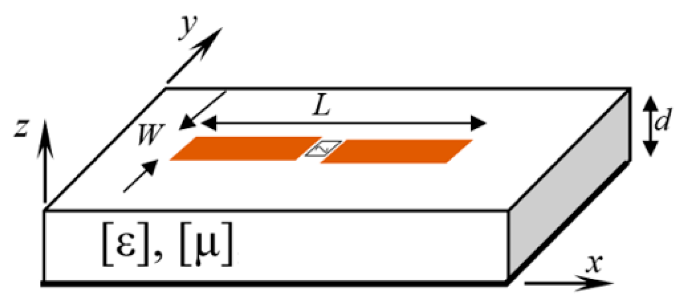
2. Analytical Formulation

Uniaxial materials have the same element in two dimensions, permittivity or permeability, and different in the third dimension. The axis along the single value direction is called the optical axis. Figure 1 shows the structure considered in this analysis. The presented configuration will be considered to establish the electric and magnetic field distributions and determine how the input impedance is affected by the uniaxial anisotropic substrate. In this analysis, the uniaxial permittivity and permeability anisotropy is given by the following expressions, respectively:
[ ε ] = ε 0 [ ε t 0 0 0 ε t 0 0 0 ε z ]
[ μ ] = μ 0 [ μ t 0 0 0 μ t 0 0 0 μ z ]
[ ε ] and [ μ ] are, respectively, the tensors of the relative permittivity and permeability, which are assumed to be low-frequency dispersive in the microwave frequency band.
First, assuming the temporal dependence e j ω t of the fields and applying Maxwell’s equations in the Fourier domain with / x j α and / y j β assumptions, we derive the expressions of the transverse components of the electromagnetic field E ˜ z and H ˜ z , two decoupled homogeneous differential wave equations of the second order are obtained:
2 E ˜ z z 2 γ e 2 E ˜ z = 0
2 H ˜ z z 2 γ h 2 H ˜ z = 0
The dispersion relations are found to be as follows:
γ e = ( ε t ε z ( α 2 + β 2 ) κ 0 2 ε t μ t )
γ h = ( μ t μ z ( α 2 + β 2 ) κ 0 2 ε t μ t )
γ e 2 and γ h 2 represent the propagation constants of the TM and TE transverse modes, respectively. κ 0 is the free space wavenumber and ω is the angular frequency. α and β are the Fourier variables corresponding to the space domain wavenumbers κ x and κ y .

3. Method of Solution

Extensive mathematical manipulations of Maxwell’s equations result in the wave Equations (2a) and (2b), which admit a general solution of the form (3a) and (3b). On the other hand, for the region above the substrate (air region), the spectral components are decreasing waves with z, for which the solutions (4a) and (4b) are assumed.
E ˜ z ( γ e , z ) = A e cosh ( γ e z ) + B e sinh ( γ e z )
H ˜ z ( γ h , z ) = A h sinh ( γ h z ) + B h cosh ( γ h z )
with A e , B e , A h and B h are complex constants
E ˜ z ( γ 0 , z ) = C e e γ 0 ( z d )
H ˜ z ( γ 0 , z ) = C h e γ 0 ( z d )
and
γ 0 = ( α 2 + β 2 ) κ 0 2
and C e and C h are complex constants.
The boundary conditions have been applied to obtain the dyadic Green’s functions. In the configuration of narrow dipoles, it is assumed that the width of the strip is very small, thus, the transverse current density in the y-direction is usually neglected [31]. Therefore, only the expression of G ˜ x x is presented:
G ˜ x x = j ω ε 0 ( α 2 + β 2 ) [ α 2 γ 0 γ e ( γ 0 ε t coth ( γ e d ) + γ e ) β 2 κ 0 2 μ t ( γ h coth ( γ h d ) + μ t γ 0 ) ]
Mathematical development of the resulting equations lead to the formulation of the estimated electric field at the interface between the two regions as functions of the current densities J ˜ x and J ˜ y . The expressions of the x-, y- and z-components of the electric and magnetic fields in the 1st and 2nd regions can be expressed as follows:
  • 1st region:
    E ˜ x 1 ( α , β , z ) = j α 2 + β 2 1 ω ε 0 ( α γ e 2 γ 0 Se × A e + β κ 0 2 μ t Sh × A h )
    E ˜ y 1 ( α , β , z ) = j α 2 + β 2 1 ω ε 0 ( β γ e 2 γ 0 Se × A e α κ 0 2 μ t Sh × A h )
    E ˜ z 1 ( α , β , z ) = γ 0 γ e c ε t ω ε 0 ε z Se × A e
    H ˜ x 1 ( α , β , z ) = 1 α 2 + β 2 ( β γ 0 ε t γ e c Se × A e α γ h c Sh × A h )
    H ˜ y 1 ( α , β , z ) = 1 α 2 + β 2 ( α γ 0 ε t γ e c Se × A e β γ h c Sh × A h )
    H ˜ z 1 ( α , β , z ) = j μ t μ z Sh × A h
  • 2nd region:
    E ˜ x 2 ( α , β , z ) = j e γ 0 ( z d ) α 2 + β 2 1 ω ε 0 [ α γ 0 γ e 2 A e + β μ t κ 0 2 A h ]
    E ˜ y 2 ( α , β , z ) = j e γ 0 ( z d ) α 2 + β 2 1 ω ε 0 [ β γ 0 γ e 2 A e α μ t κ 0 2 A h ]
    E ˜ z 2 ( α , β , z ) = γ e 2 ω ε 0 A e e γ 0 ( z d )
    H ˜ x 2 ( α , β , z ) = e γ 0 ( z d ) α 2 + β 2 ( β γ e 2 A e + μ t α γ 0 A h )
    H ˜ y 2 ( α , β , z ) = e γ 0 ( z d ) α 2 + β 2 ( α γ e 2 A e + β μ t γ 0 A h )
    H ˜ z 2 ( α , β , z ) = j μ t A h e γ 0 ( z d )
    where J ˜ x and J ˜ y are the Fourier transforms of the current densities, and
    A e = α J ˜ x + β J ˜ y ( γ e 2 + γ 0 ε t γ e coth ( γ e d ) )
    A h = β J ˜ x α J ˜ y ( γ h coth ( γ h d ) + γ 0 μ t )
    γ e c = γ e coth ( γ e d )
    γ h c = γ h coth ( γ h d )
    Se = sinh ( γ e z ) sinh ( γ e d )
    Sh = sinh ( γ h z ) sinh ( γ h d )

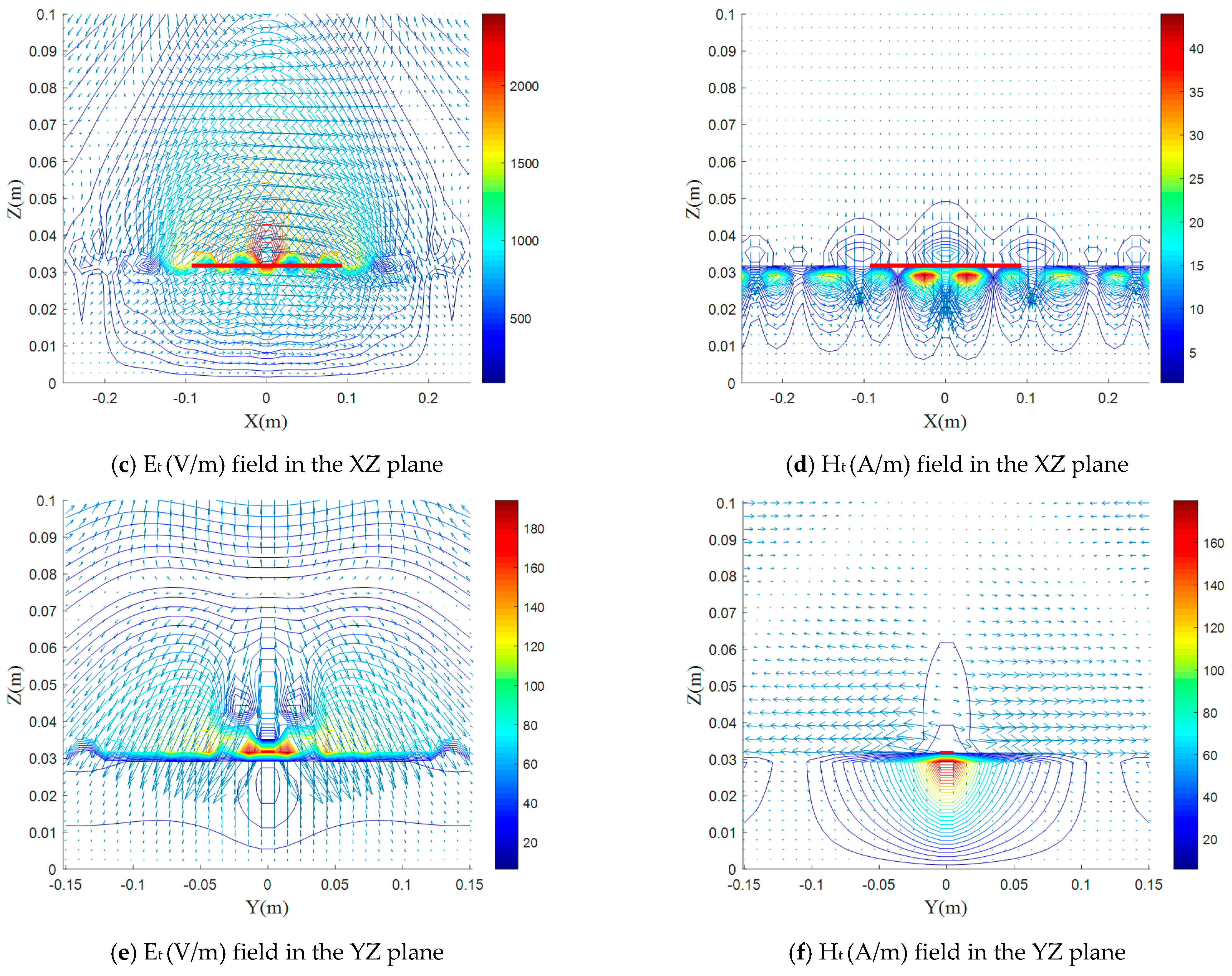
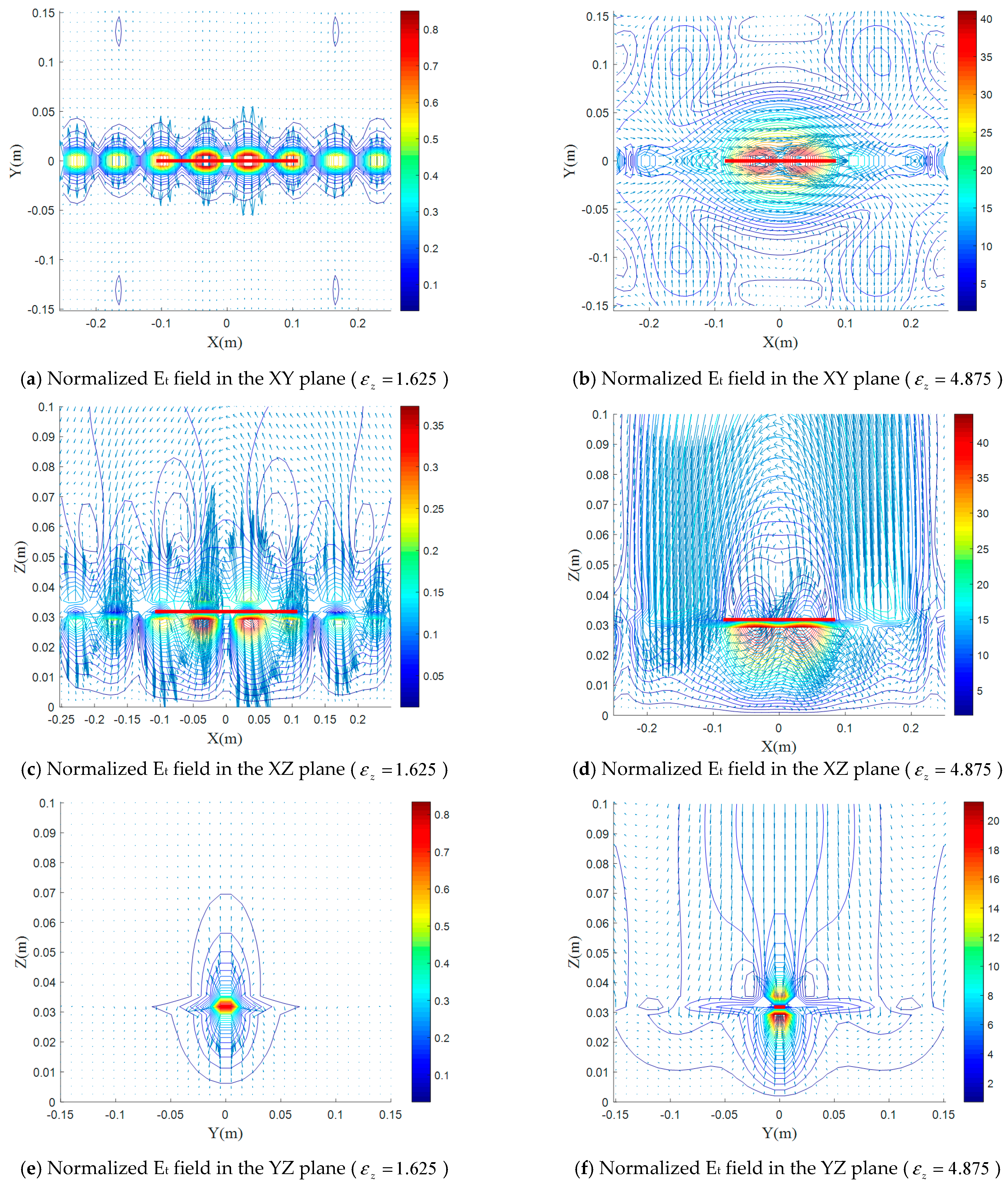
4. Fields Computations

The spectral domain immittance functions are used to evaluate the configuration shown in Figure 1. In particular, we seek to determine the distribution of the electric and magnetic fields on a printed dipole embedded on an anisotropic layer. The dipole has length L and width W. The electromagnetic field components are deduced after satisfying the boundary conditions on the printed dipole.
As mentioned in the section above, G ˜ x x represents the Green’s function in the spectral domain and the Green’s function in the spatial domain is merely the inverse Fourier transform. The components of the electric and magnetic fields in each region can be written in the spatial domain as [42,43]:
Φ ( x , y , z ) = 1 ( 2 π ) 2 Φ ˜ ( α , β , z ) e j ( α x + β y ) d α d β
With Formulation (9), a specific structure was chosen to be examined. The electromagnetic field expressions are derived in the spatial domain via the inverse Fourier transform. The Matlab® software [44] is used to plot the fields distributions.

5. Numerical Results
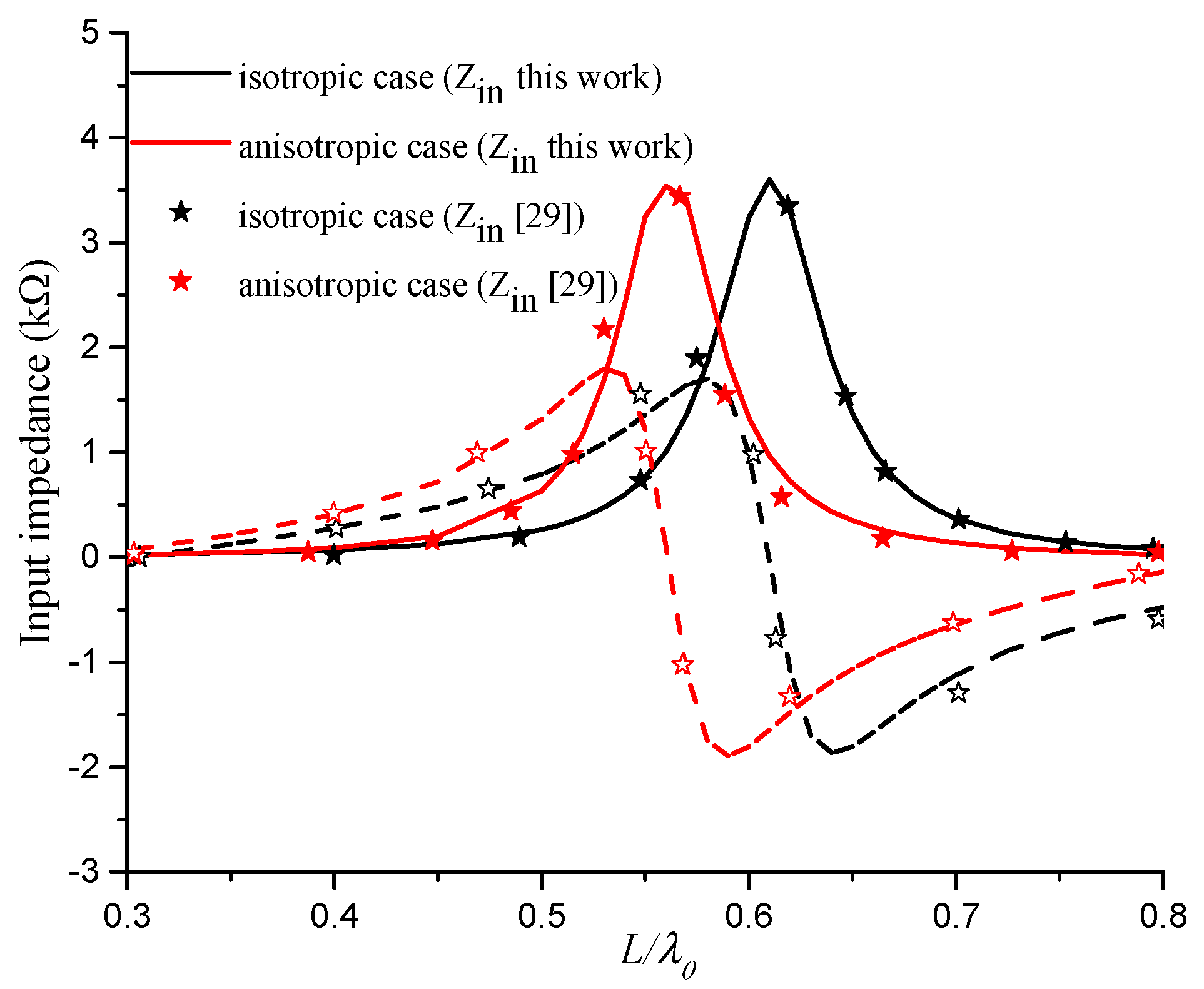
In this work, we are firstly interested in the input impedance, the resonant length of the dipole and secondly in the distribution of the electromagnetic fields. Before discussing the results obtained for the uniaxial anisotropy case, a validation of the calculation code, elaborated in Matlab, is carried out through a comparison with published literature.

5.1. Validation

In this subsection, we consider the basic configuration of a monolayer 0.1060λ0 thick substrate planar dipole antenna. The objective of this work is to analyze the effects of different electromagnetic parameters of the anisotropic substrate on the input impedance of the dipole, in addition to the electromagnetic field evaluation through the plotting of the electric and magnetic field distributions in the three principal planes XY, XZ, and YZ.
Calculations of a dipole structure on a uniaxial anisotropic structure have been performed. The results have been successfully compared with published ones. We initially considered the isotropic and uniaxial anisotropic cases ( ε t = ε z = 3.25 and μ t = μ z = 1) and ( ε t = 3.14, ε z = 5.12 and μ t = μ z = 1), respectively. Figure 2 depicts the input impedance (real and imaginary parts) of a planar dipole of width W = 0.0004λ0 as a function of normalized length L/λ0. These results represent a validation step of the accuracy of our calculations for both isotropic and anisotropic substrates. The representation shows good agreement with the data reported in [29]. In [29], only cases of electrical anisotropy were considered and no discussion of the effect of this component was conducted.

5.2. Electromagnetic-Field Distributions in Isotropic Case

Once the expressions for the transverse and longitudinal components are found, the electromagnetic fields expressions are evaluated. Since the processing takes place in the spectral domain, the final fields must be brought back into the spatial domain. The Matlab functions “quiver3” and “contour” are used in plotting the field lines in their arrow and equi-phase contour forms. It is clear from these results that the considered antenna structure shows the well-known shape of a dipole radiated electromagnetic field. The anisotropic results of the tangential-field lines are plotted for different planes at the equivalent resonant dipole length compared to the isotropic case. The magnitude of the electromagnetic fields are normalized with respect to the isotropic case for comparison.
In our case, we evaluate the electric and magnetic field distributions in a dipole antenna structure based on media with various uniaxial anisotropies and the effect of the different elements of the constitutive parameters. This will serve as a platform for the treatment of other cases of microwave structures based on more complex media such as: electric negative material (ENG), magnetic negative material (MNG), double negative material (DNG), and chirality.
Figure 3 shows the electric and magnetic fields arrow plots for the tangential fields components Et and Ht, in the transverse plane with respect to z-, y- and x-axis, respectively, for the isotropic case. The arrow indicates the cross-sectional field vector direction and the arrow length designates the field magnitude, and the lines indicates the equi-phase field contour forms.
From the plots, we can easily notice that the E- and H-plane are the XZ and the YZ planes (Figure 3b,c), respectively. In Figure 3a, a quite rectangular shape of the E field distribution is clearly observed due to the fringing fields close to the edge of the strip and the electric field has a small component parallel to the dipole. The electric field is not entirely confined within the dielectric substrate; it extends partially into the air above. This phenomenon is commonly referred to as fringing, as shown in Figure 3a,c,e.
The fringing E-field makes the dipole electrically longer than its real physical dimension. This is why the dipole physical length is chosen to be slightly less than half the dielectric wavelength. At resonance, the dipole electrical length must equal half the dielectric wavelength. The antenna fringing field amount is strongly related to the radiating element geometry and the substrate permittivity. Substrates with low dielectric constants allow more field fringing than do high dielectric constant-substrates [45]. It can be seen from Figure 3e, given that the direction of propagation is along z-axis, that the spacing between the lines at z = 0.75 m is equivalent to λ/4, this illustrates the concept of propagation.
Figure 3d,f show a high confinement of the H field in the substrate, due to the fact that the magnetic field is in direct relation with the electric induction, this is due to the contribution of the two dielectric constants ε r = 3.25 and μ r = 1 .

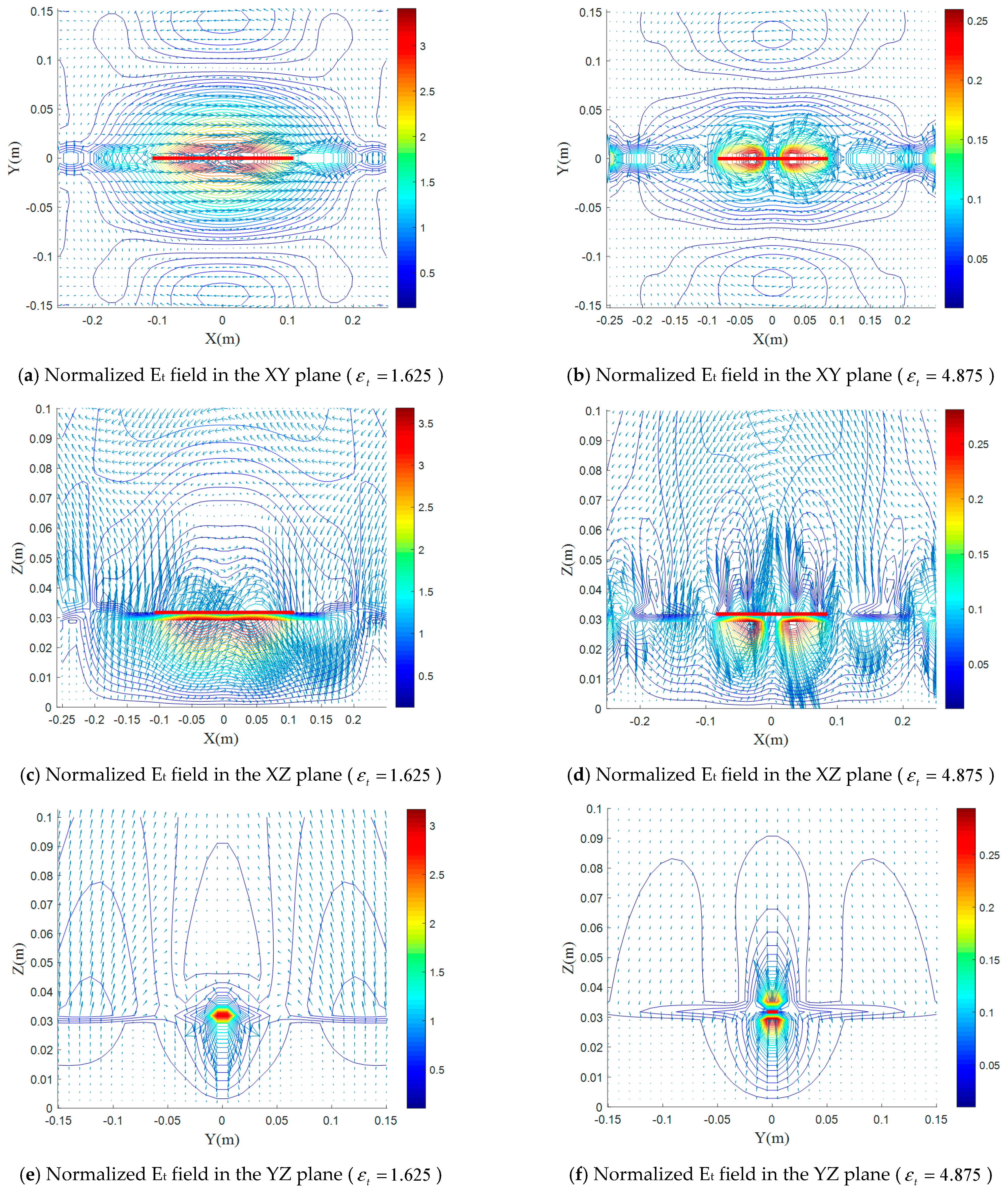
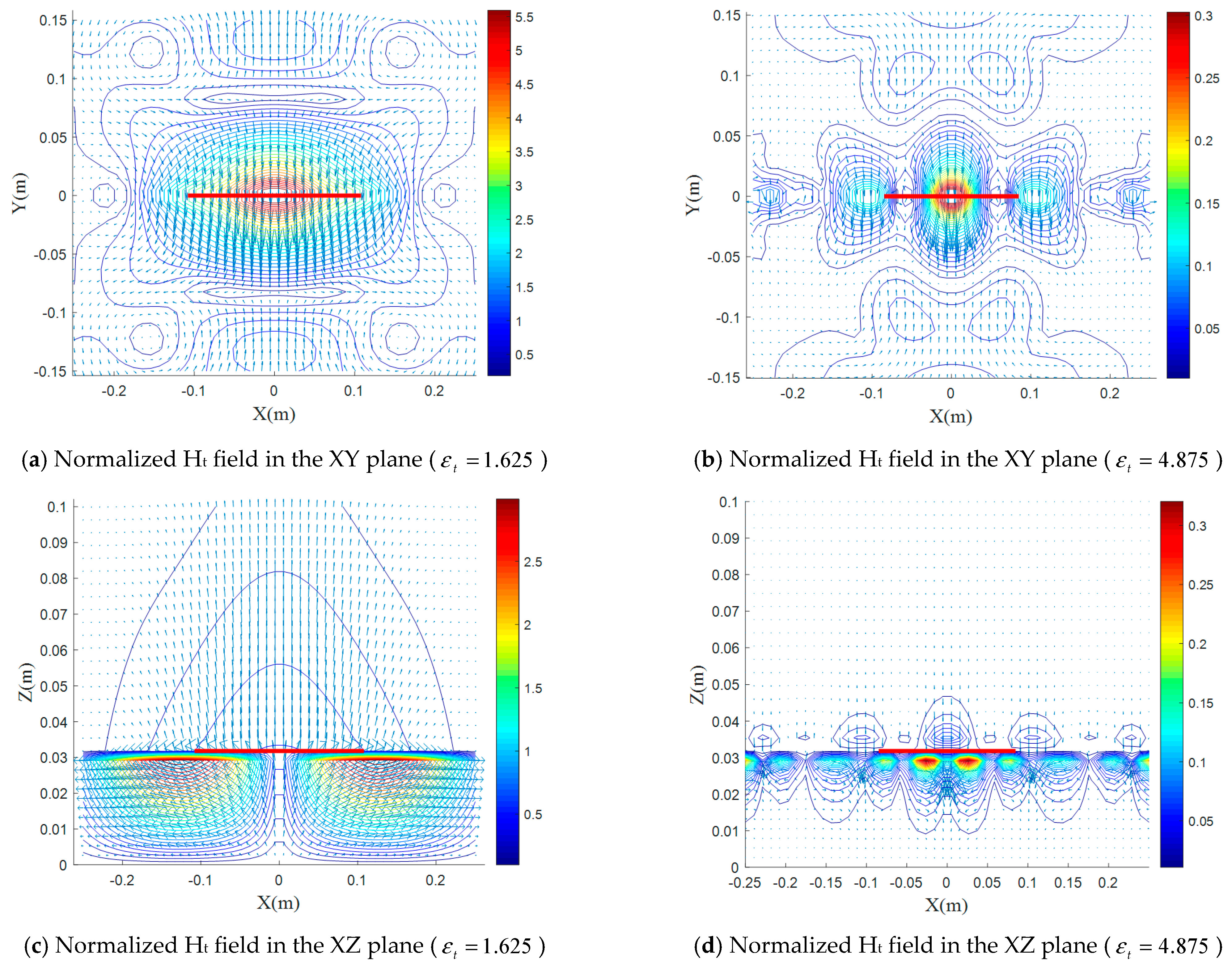
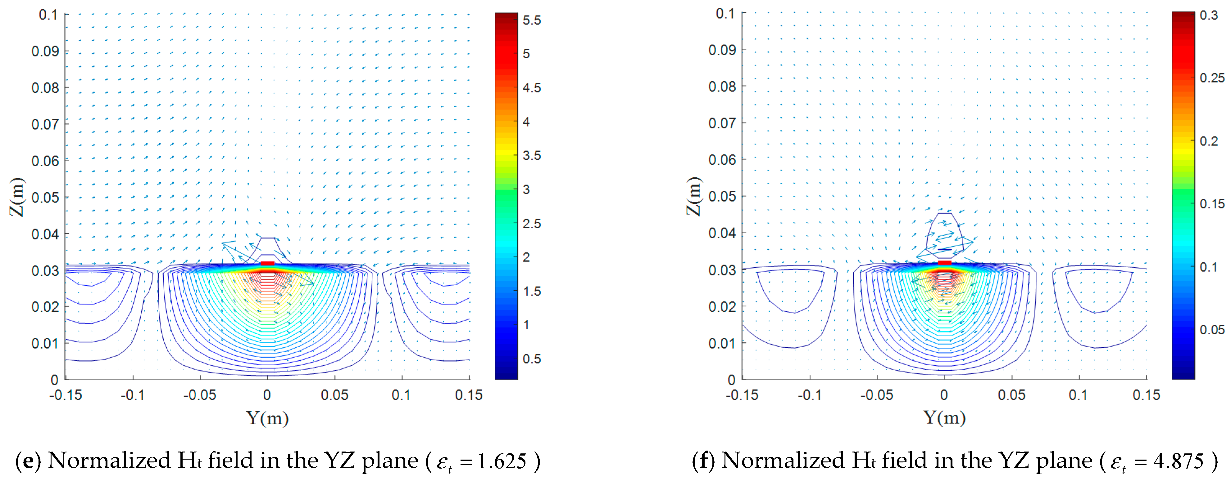
5.3. Effect of the Electrical Uniaxial Anisotropy on the Electromagnetic-Field Distributions

In this section, we examine the effect of the electrical anisotropy on the electromagnetic field distributions in the three planes, and we interpret these results through the shape of the input impedance. Figure 4a–f show the normalized tangential electric field magnitude in a color plot superimposed on the vector plots in arrow representation for various values of ε z with ε t = 3.25 , μ z = 1 and μ t = 1 in the XY, XZ, and YZ planes.
According to Figure 4 and Figure 5, we roughly notice an effect reversed in shape and different in details of the two anisotropic elements ε z and ε t . A decrease in ε z up to 40% leads to a slight decrease and the E-plane decreases its max by 50%, while an increase of 40% reveals a significant increase in the electric field in the E- and H-plane.
A decrease of 40% in ε t leads to an almost identical increase (3 times) of the electric field maximum, while for an increase of 40%, an identical decrease of the maximum in all three planes is noticed (64%). As a consequence of this result, and to improve the dipole radiation, it is necessary to strongly minimize ε t and increase, in the possibility, ε z . From Figure 4a,b and Figure 5a,b, it can be seen that for the case ( ε t = 1.625 ), a maximum electric field exceeds 0.2 m, when the element ε t is reduced, this agrees well with the literature [45].
According to Figure 4c,d and Figure 5c,d, the electric field lines are condensed since they are presented, in this case, in the E plane, and we can see that the component Ex is the most important in the cases of Figure 4d and Figure 5c from Figure 4e,f and Figure 5e,f, it is clear that the most important part of the electric field is confined in the dielectric and around the dipole.
From Figure 6 and Figure 7, we notice that the contribution of the two electrical anisotropic components ε z and ε t on the magnetic field distribution is almost the same as that on the electric field, except that the magnetic field in the E plane undergoes more decrease in the case (XZ plane ε z = 1.625 (Figure 6c) and XZ plane ε t = 1.625 (Figure 7c) compared to the other planes) and a slight increase for the case XZ plane ε z = 4.875 (Figure 6d) compared to the other planes) and for the case ε t = 4.875 , the decrease is almost the same (Figure 7b,f).

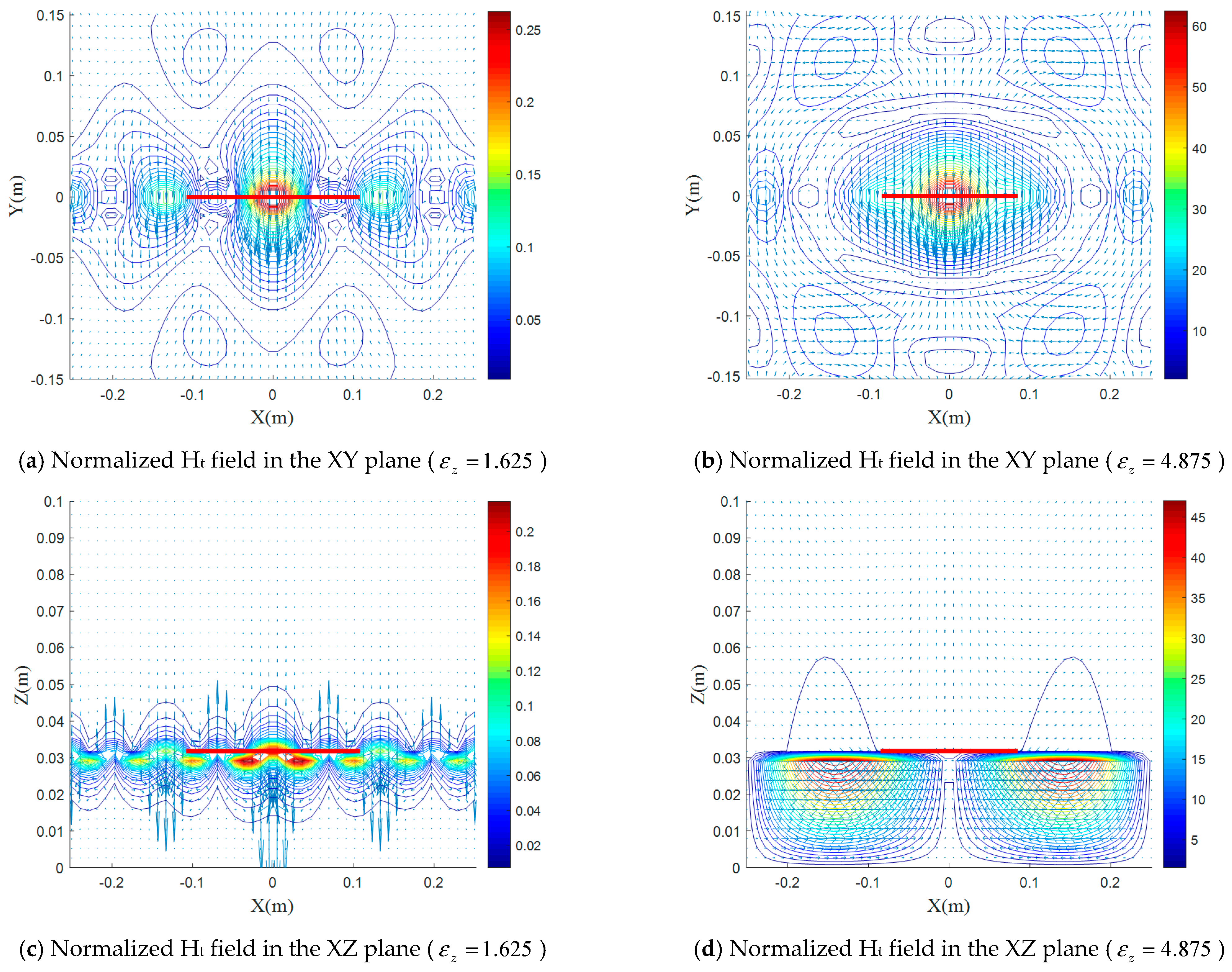
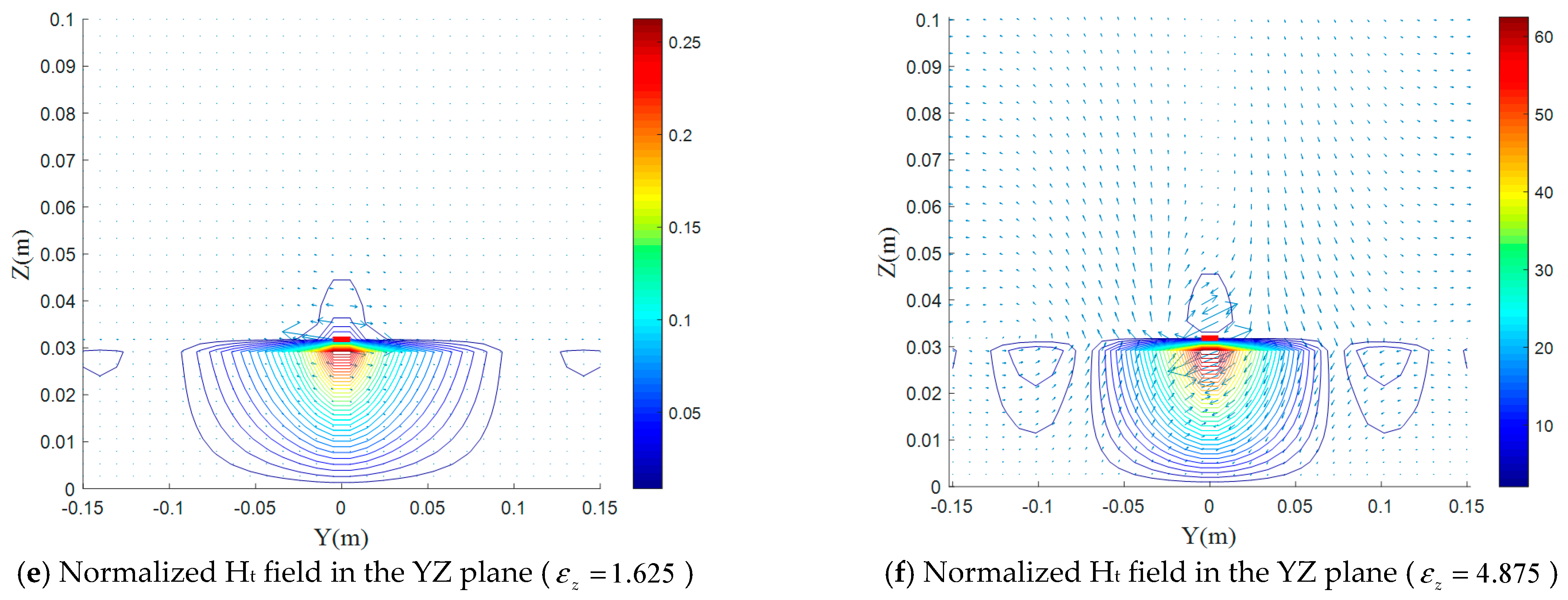
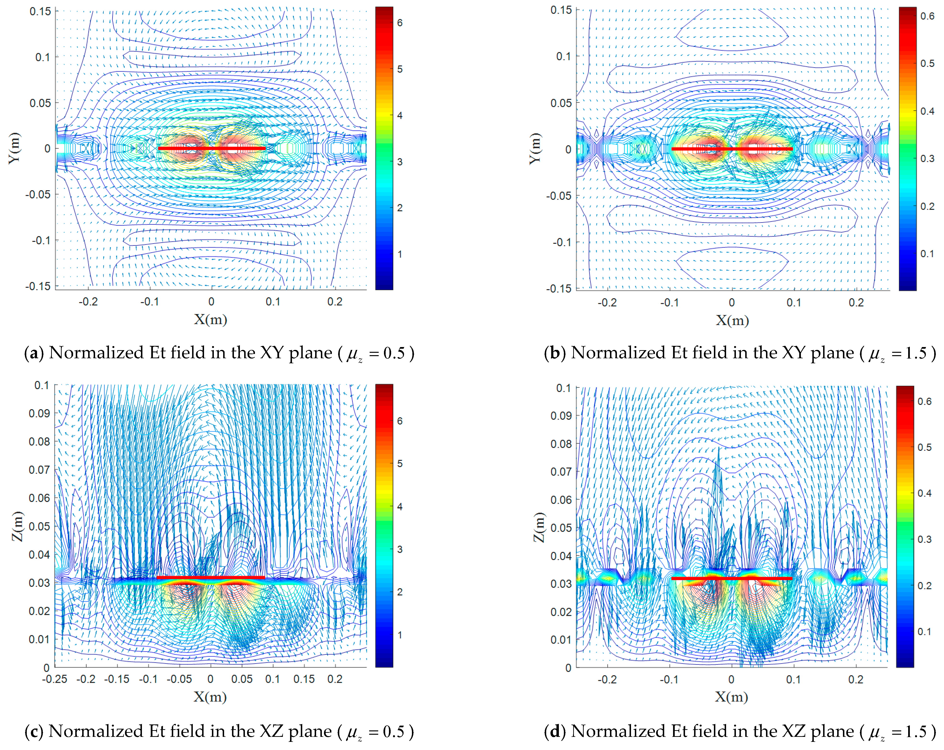
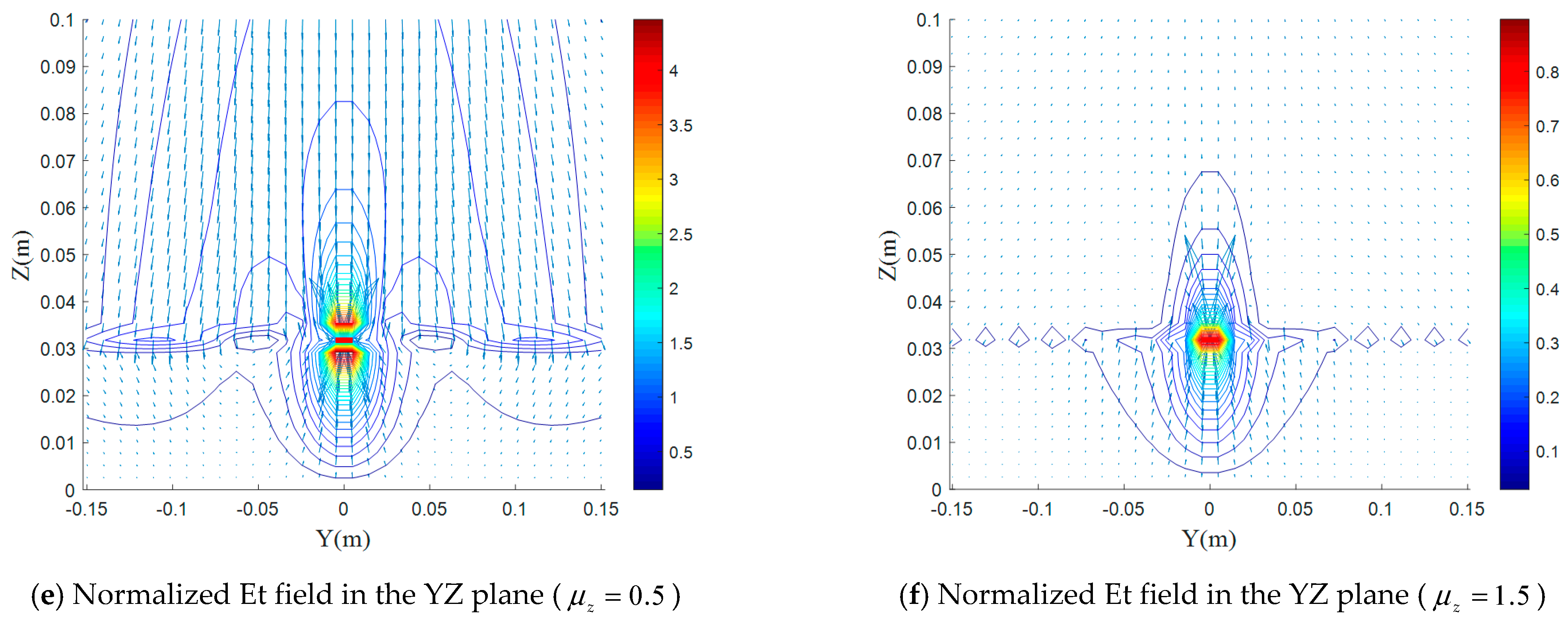
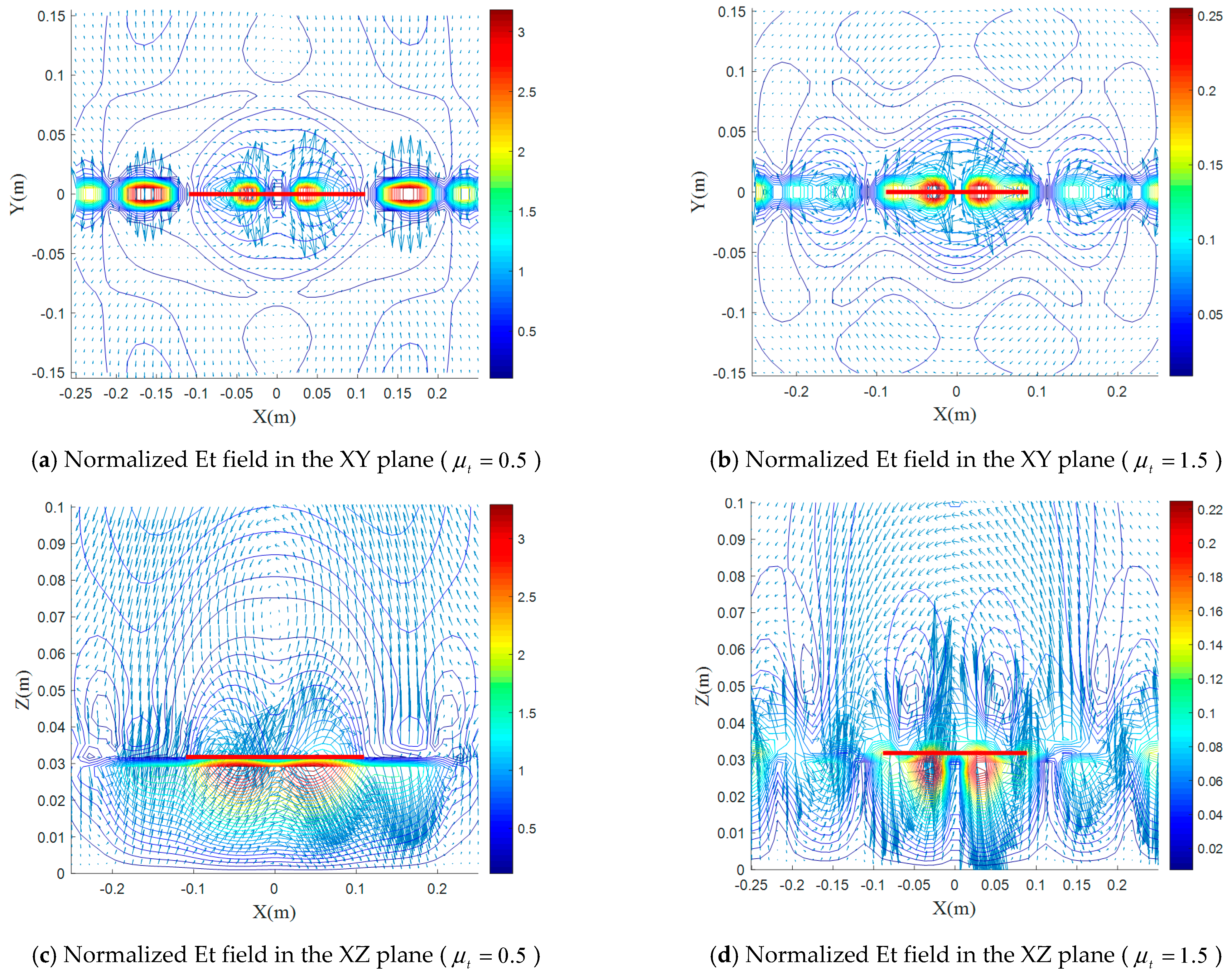
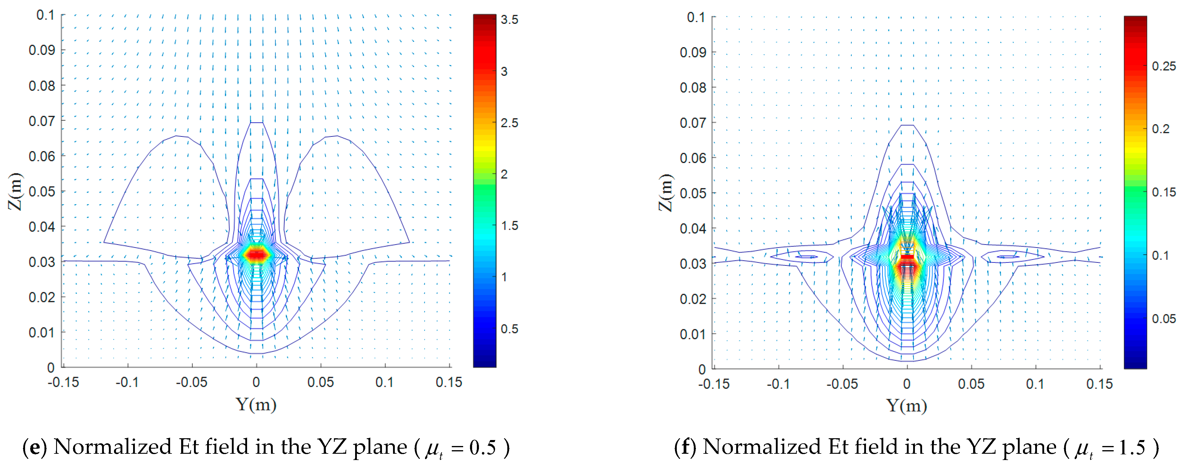
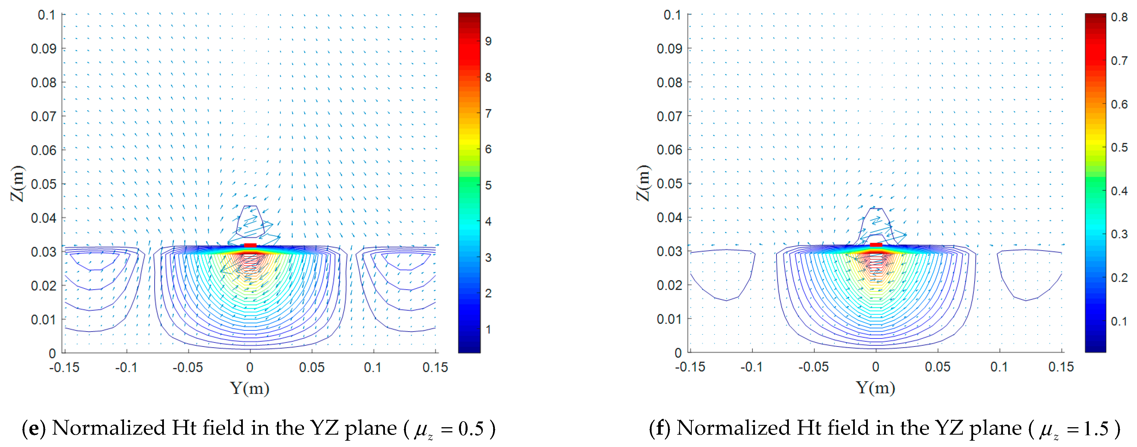
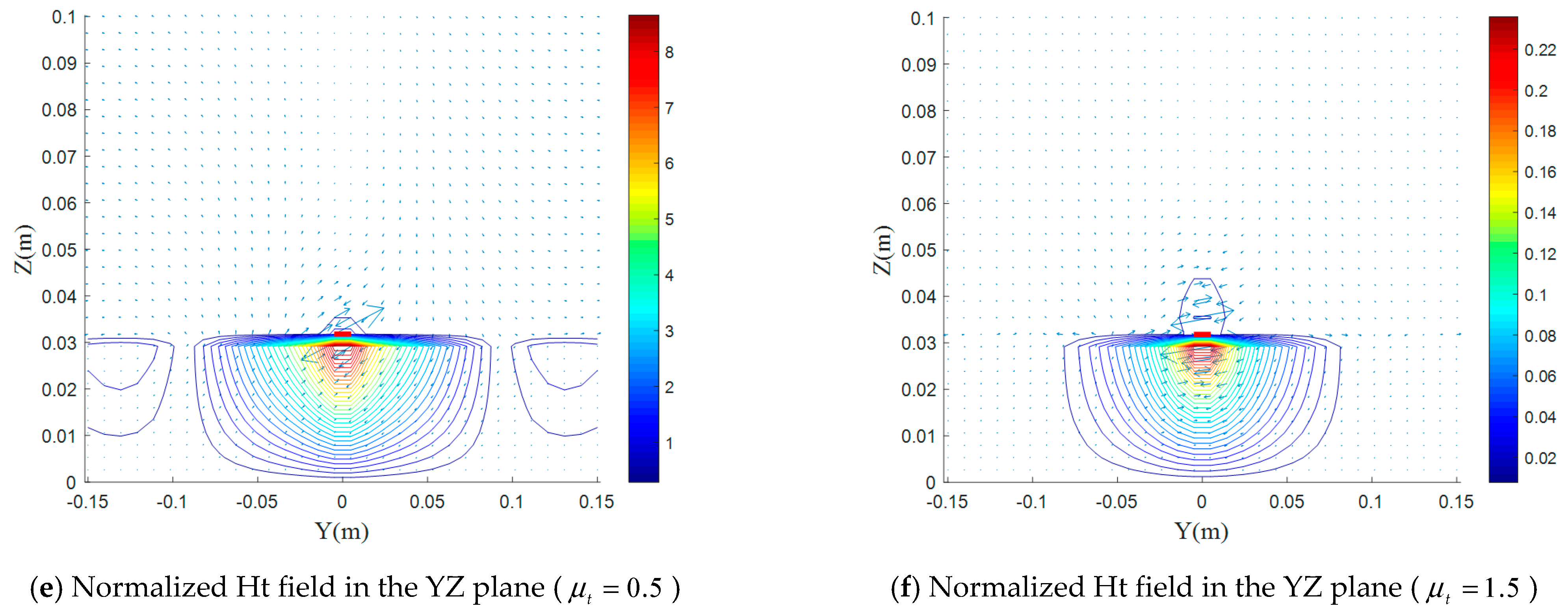
5.4. Effect of the Magnetic Uniaxial Anisotropy on Electromagnetic-Field Distributions

Figure 8, Figure 9, Figure 10 and Figure 11 show the effect of the uniaxial electrical anisotropy on electric and magnetic field distributions.
It can be seen from Figure 4, Figure 5 and Figure 8 that the effect of the permeability component μ z on the line shape and distribution of the electric field is similar to that of ε z , but in terms of value and quantity, it has the same effect as ε t . However in the case of the μ t component, and according to Figure 4, Figure 5 and Figure 9, the effect of μ t component is close in shape and quantity to that of ε t .
From here, we can note that the four ( ε z , ε t , μ t and μ z ) constitutive components have a different contribution to each other, and this is mainly due to the dipole antenna configurations and its positioning.
From Figure 8, Figure 9, Figure 10 and Figure 11, we can see that the two components μ t and μ z have a different effect than the two permittivity components.
The increase of μ t and μ z leads to a decrease of the fields maximum compared to the isotropic case, while when ε z increases, the maximum E increases strongly. Moreover, the effect of the two components μ t and μ z is close to that of ε t in form and magnitude. This is due to the lines of the magnetic field, which rotates around the dipole (YZ plane), indicating that the maximum magnetic field interaction is through the two components μ t and μ z as well as with ε t .

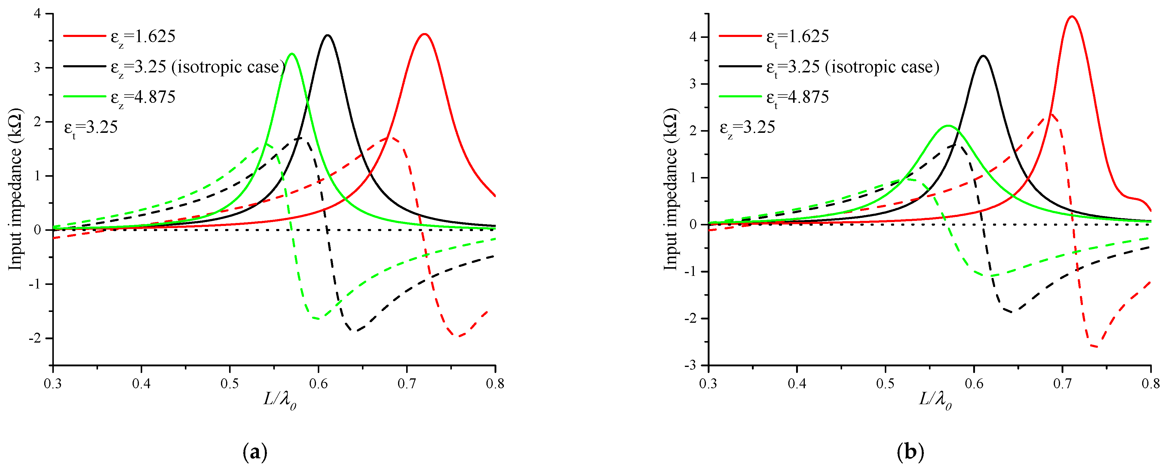
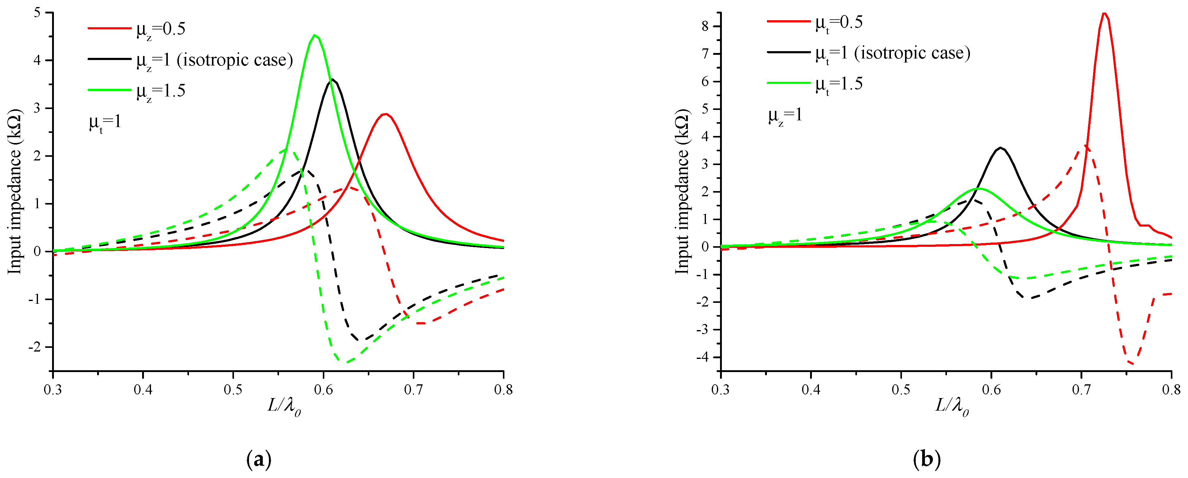
5.5. Effect of the Uniaxial Anisotropy on Input Impedance

Figure 12a shows the effect of ε z on the input impedance. It consists in shifting the resonant length of the dipole antenna with a slight change in its peak, while ε t affects significantly the magnitude of the input impedance with an increase and decrease of its peak, from 3 kΩ for ε t = 3.25 to 5 kΩ for ε t = 1.625 and 3 kΩ for ε t = 3.25 to 2.5 kΩ for ε t = 4.875 , all with a slight shift in the resonant length (Figure 12b).
In Figure 13a,b, the effect of the two components of permeability μ z and μ t does not resemble that of the permittivity components ε z and ε t . An increase in μ z results in an increase in the input impedance peak, with a decrease in the resonance frequency. The effect of the permeability component μ t is reversed in this case, where an increase in the μ t component leads to a significant increase in the resonance frequency with a decrease in the peak value of input impedance.
In the case ε z = 1.625 , a decrease of 35% of the maximum of the electric field is observed in the XZ plane (E plane), according to Figure 4c, accompanied by a close decrease in the magnetic field (27%) in the YZ plane (H plane), according to Figure 6e. This is translated by a slight increase (5.5 and 3.5 times) of the input impedance (Figure 12a). However, in the case for ε t = 1.625 , the maximum of the magnetic field in the H-plane (Figure 7e) is almost twice that of the electric field in the E-plane (Figure 5c) and for ε t = 4.875 , a ratio between the field maxima is 1.4. This illustrates the effect of ε t on the input impedance (Figure 12b). In this case, the maximum of the magnetic field is greater than that of the electric field; this reveals the effect of the component ε t on input impedance.
Figure 13a,b show the effect of the uniaxial magnetic anisotropy on the dipole input impedance. For the cases μ z = 0.5 and μ z = 1.5 , the same ratio of increase and decrease between the electric field E and the magnetic field H (normalized values 7 times to 9 times (Figure 10), 0.8 to 0.65 (Figure 8), respectively) led to an almost identical decrease and increase, respectively, in input impedance (Figure 13a).
In the case μ t = 0.5 , a 9-times increase of the H field maximum, in the YZ plane (Figure 11e), compared to the isotropic case, is accompanied by a 6-times increase of the E field maximum in the XZ plane (Figure 9c); this is translated by a strong increase of the input impedance (Figure 13b). On the other hand, in the case μ t = 1.5 , an almost identical decrease of the H- and E-field maxima (0.25 (Figure 11f) and 0.22 (Figure 9d), respectively, in the YZ XZ plane); this is translated by a decrease of input impedance (Figure 13b).
To summarize, we notice that the choice of the optical axis of the uniaxial anisotropy and the geometry of the printed dipole lead to an asymmetrical Green’s tensor, relating the electric field to the current density through the four constituent parameters ε t , ε z , μ t and μ z . This is the factor behind the difference registered between the effects of these components, in addition to the electromagnetic field distributions.

6. Conclusions

In this paper, we presented a theoretical study for the investigation of the electromagnetic field distributions and the input impedance of a printed dipole antenna structure loaded on a uniaxial anisotropic medium. The presentation of the electromagnetic field distributions, for which some examples have been shown here, provides a better understanding of the constitutive parameters ( ε t , ε z , μ t and μ z ) contributions. Furthermore, the electrical and magnetic uniaxial anisotropy offers more degrees of freedom and further flexibility to realize a good direct matching effect on the input impedance. This show that the complex media present a great potential in the design of innovative microwave components. It constitutes a starting point for further works to a better understanding of the behavior of the electromagnetic field in anisotropic and bianisotropic media and many more interesting results are expected.

Author Contributions

Design and concept, M.L.B., D.S., and C.Z.; methodology, C.Z., I.E., and M.A.; investigation, M.A. and F.F.; resources, C.Z. and I.E.; writing—original draft preparation, M.L.B., C.Z., and D.S.; writing—review and editing, I.E., R.A.A.-A., and M.A.; supervision, R.A.A.-A. and E.L.; project administration, J.R. and E.L., formal analysis, M.L.B. and C.Z. All authors have read and agreed to the published version of the manuscript.

Funding

This project received funding in part from the DGRSDT (Direction Générale de la Recherche Scientifique et du Développement Technologique), MESRS (Ministry of Higher Education and Scientific Research), Algeria. This work is also funded by the FCT/MEC through national funds and when applicable co-financed by the ERDF, under the PT2020 Partnership Agreement, the UID/EEA/50008/2019 project.

Data Availability Statement

All data are included within manuscript.

Acknowledgments

This work was supported in part by the DGRSDT (Direction Générale de la Recherche Scientifique et du Développement Technologique), MESRS (Ministry of Higher Education and Scientific Research), Algeria. This work is part of the POSITION-II project funded by the ECSEL joint Undertaking under grant number Ecsel-7831132-Postitio-II-2017-IA. This work is partially supported by RTI2018-095499-B-C31, funded by Ministerio de Ciencia, Innovación y Universidades, Gobierno de España (MCIU/AEI/FEDER, UE).

Conflicts of Interest

The authors declare no conflict of interest.

References

  1. Kirilenko, A.A.; Steshenko, S.O.; Derkach, V.N.; Prikolotin, S.A.; Kulik, D.Y.; Prosvirnin, S.; Mospan, L.P. Rotation of the polarization plane by double-layer planar-chiral structures. Review of the results of theoretical and experimental studies. Radioelectron. Commun. Syst. 2017, 60, 193–205. [Google Scholar] [CrossRef]
  2. Akdagli, A. Behaviour of Electromagnetic Waves in Different Media and Structures, 1st ed.; BoD–Books on Demand: Rijeka, Croatia, 2011. [Google Scholar]
  3. Guo, B. Photonic band gap structures of obliquely incident electromagnetic wave propagation in a one-dimension absorptive plasma photonic crystal. Phys. Plasmas 2009, 16, 043508. [Google Scholar] [CrossRef]
  4. Krowne, C.M. Left-handed material anisotropy effect on guided wave electromagnetic fields. J. Appl. Phys. 2006, 99, 044914. [Google Scholar] [CrossRef]
  5. Krowne, C.M.; Daniel, M. Electromagnetic field behavior in dispersive isotropic negative phase velocity/negative refractive index guided wave structures compatible with millimeter-wave monolithic integrated circuits. J. Nanomater. 2007, 2007, 054568. [Google Scholar] [CrossRef]
  6. Krowne, C.M. Electromagnetic-field theory and numerically generated results for propagation in left-handed guided-wave single-microstrip structures. IEEE Trans. Microw. Theory Tech. 2003, 51, 2269–2283. [Google Scholar] [CrossRef]
  7. Krowne, C.M. Electromagnetic distributions demonstrating asymmetry using a spectral-domain dyadic Green’s function for ferrite microstrip guided-wave structures. IEEE Trans. Microw. Theory Tech. 2005, 53, 1345–1361. [Google Scholar] [CrossRef]
  8. Zebiri, C.; Lashab, M.; Benabdelaziz, F. Effect of anisotropic magneto-chirality on the characteristics of a microstrip resonator. IET Microw. Antennas Propag. 2010, 4, 446–452. [Google Scholar] [CrossRef]
  9. Zebiri, C.; Lashab, M.; Benabdelaziz, F. Rectangular microstrip antenna with uniaxial bi-anisotropic chiral substrate–superstrate. IET Microw. Antennas Propag. 2011, 5, 17–29. [Google Scholar] [CrossRef]
  10. Sayad, D.; Zebiri, C.; Daoudi, S.; Benabdelaziz, F. Analysis of the effect of a gyrotropic anisotropy on the phase constant and characteristic impedance of a shielded microstrip line. Adv. Electromagn. 2019, 8, 15–22. [Google Scholar] [CrossRef]
  11. Heydari, M.B.; Ahmadvand, A. A novel analytical model for a circularly-polarized; ferrite-based slot antenna by solving an integral equation for the electric field on the circular slot. Waves Random Complex Media 2020, 1–20. [Google Scholar] [CrossRef]
  12. Lee, W.; Hong, Y.K.; Choi, M.; Won, H.; Lee, J.; Park, S.O.; Yoon, H.S. Ferrite-cored patch antenna with suppressed harmonic radiation. IEEE Trans. Antennas Propag. 2018, 66, 3154–3159. [Google Scholar] [CrossRef]
  13. Kamra, V.; Dreher, A. Efficient analysis of multiple microstrip transmission lines with anisotropic substrates. IEEE Microw. Wirel. Compon. Lett. 2018, 28, 636–638. [Google Scholar] [CrossRef]
  14. Buzov, A.L.; Buzova, M.A.; Klyuev, D.S.; Mishin, D.V.; Neshcheret, A.M. Calculating the Input Impedance of a Microstrip Antenna with a Substrate of a Chiral Metamaterial. J. Commun. Technol. Electron. 2018, 63, 1259–1264. [Google Scholar] [CrossRef]
  15. Klyuev, D.S.; Minkin, M.A.; Mishin, D.V.; Neshcheret, A.M.; Tabakov, D.P. Characteristics of Radiation from a Microstrip Antenna on a Substrate Made of a Chiral Metamaterial. Radiophys. Quantum Electron. 2018, 61, 445–455. [Google Scholar] [CrossRef]
  16. Hu, Y.; Fang, Y.; Wang, D.; Zhan, Q.; Zhang, R.; Liu, Q.H. The scattering of electromagnetic fields from anisotropic objects embedded in anisotropic multilayers. IEEE Trans. Antennas Propag. 2019, 67, 7561–7568. [Google Scholar] [CrossRef]
  17. Zebiri, C.; Daoudi, S.; Benabdelaziz, F.; Lashab, M.; Sayad, D.; Ali, N.T.; Abd-Alhameed, R.A. Gyro-chirality effect of bianisotropic substrate on the operational of rectangular microstrip patch antenna. Int. J. Appl. Electromagn. Mech. 2016, 51, 249–260. [Google Scholar] [CrossRef]
  18. Zebiri, C.; Benabdelaziz, F.; Sayad, D. Surface waves investigation of a bianisotropic chiral substrate resonator. Prog. Electromagn. Res. 2012, 40, 399–414. [Google Scholar] [CrossRef] [Green Version]
  19. Eroglu, A.; Lee, J.K. Far field radiation from an arbitrarily oriented Hertzian dipole in the presence of a layered anisotropic medium. IEEE Trans. Antennas Propag. 2005, 53, 3963–3973. [Google Scholar] [CrossRef]
  20. Sayad, D.; Benabdelaziz, F.; Zebiri, C.; Daoudi, S.; Abd-Alhameed, R.A. Spectral domain analysis of gyrotropic anisotropy chiral effect on the input impedance of a printed dipole antenna. Prog. Electromagn. Res. 2016, 51, 1–8. [Google Scholar] [CrossRef] [Green Version]
  21. Braaten, B.D.; Rogers, D.A.; Nelson, R.M. Multi-conductor spectral domain analysis of the mutual coupling between printed dipoles embedded in stratified uniaxial anisotropic dielectrics. IEEE Trans. Antennas Propag. 2012, 60, 1886–1898. [Google Scholar] [CrossRef]
  22. Soares, A.; Fonseca, S.B.D.A.; Giarola, A. The effect of a dielectric cover on the current distribution and input impedance of printed dipoles. IEEE Trans. Antennas Propag. 1984, 32, 1149–1153. [Google Scholar] [CrossRef]
  23. Nelson, R.M.; Rogers, D.A.; D’Assuncao, A.G. Resonant frequency of a rectangular microstrip patch on several uniaxial substrates. IEEE Trans. Antennas Propag. 1990, 38, 973–981. [Google Scholar] [CrossRef]
  24. Davidson, D.B.; Aberle, J.T. An introduction to spectral domain method-of-moments formulations. IEEE Antennas Propag. Mag. 2004, 46, 11–19. [Google Scholar] [CrossRef]
  25. Wait, J. Fields of a horizontal dipole over a stratified anisotropic half-space. IEEE Trans. Antennas Propag. 1966, 14, 790–792. [Google Scholar] [CrossRef]
  26. Kong, J.A. Electromagnetic fields due to dipole antennas over stratified anisotropic media. Geophysics 1972, 37, 985–996. [Google Scholar] [CrossRef] [Green Version]
  27. Tang, C.M. Electromagnetic fields due to dipole antennas embedded in stratified anisotropic media. IEEE Trans. Antennas Propag. 1979, 27, 665–670. [Google Scholar] [CrossRef]
  28. Lee, J.K.; Kong, J.A. Dyadic Green’s functions for layered anisotropic medium. Electromagnetics 1983, 3, 111–130. [Google Scholar] [CrossRef]
  29. Braaten, B.D.; Nelson, R.M.; Rogers, D.A. Input impedance and resonant frequency of a printed dipole with arbitrary length embedded in stratified uniaxial anisotropic dielectrics. IEEE Antennas Wirel. Propag. Lett. 2009, 8, 806–810. [Google Scholar] [CrossRef]
  30. Eroglu, A.; Lee, Y.H.; Lee, J.K. Dyadic Green’s functions for multi-layered uniaxially anisotropic media with arbitrarily oriented optic axes. IET Microw. Antennas Propag. 2011, 5, 1779–1788. [Google Scholar] [CrossRef]
  31. Wang, N.; Wang, G.P. Effective medium theory with closed-form expressions for bi-anisotropic optical metamaterials. Opt. Express 2019, 27, 23739–23750. [Google Scholar] [CrossRef]
  32. Erturk, V.B.; Rojas, R.G. Efficient analysis of input impedance and mutual coupling of microstrip antennas mounted on large coated cylinders. IEEE Trans. Antennas Propag. 2003, 51, 739–749. [Google Scholar] [CrossRef]
  33. leukenov, S.K.; Assilbekova, A.M. Surface of wave vectors of electromagnetic waves in anisotropic dielectric media with rhombic symmetry. Telecommun. Radio Eng. 2017, 76, 1231–1238. [Google Scholar] [CrossRef]
  34. Sayad, D.; Zebiri, C.; Elfergani, I.; Rodriguez, J.; Abobaker, H.; Ullah, A.; Benabdelaziz, F. Complex bianisotropy effect on the propagation constant of a shielded multilayered coplanar waveguide using improved full generalized exponential matrix technique. Electronics 2020, 9, 243. [Google Scholar] [CrossRef] [Green Version]
  35. Sayad, D.; Zebiri, C.; Elfergani, I.; Rodriguez, J.; Abd-Alhameed, R.A.; Benabdelaziz, F. Analysis of Chiral and Achiral Medium Based Coplanar Waveguide Using Improved Full Generalized Exponential Matrix Technique. Radioengineering 2020, 29, 591–600. [Google Scholar] [CrossRef]
  36. Zebiri, C.; Sayad, D. Effect of bianisotropy on the characteristic impedance of a shielded microstrip line for wideband impedance matching applications. Waves Random Complex Media 2020, 1–14. [Google Scholar] [CrossRef]
  37. Nakano, H.; Kerner, S.R.; Alexopoulos, N.G. The moment method solution for printed wire antennas of arbitrary configuration. IEEE Trans. Antennas Propag. 1988, 36, 1667–1674. [Google Scholar] [CrossRef] [Green Version]
  38. Lee, H.; Tripathi, V.K. Spectral domain analysis of frequency dependent propagation characteristics of planar structures on uniaxial medium. IEEE Trans. Microw. Theory Tech. 1982, 30, 1188–1193. [Google Scholar]
  39. Harrington, R.F. Field Computation by Moment Methods; IEEE Press, Inc.: New York, NY, USA, 1992. [Google Scholar]
  40. Itoh, T. Numerical Techniques for Microwave and Millimeter Wave Passive Structures, 1st ed.; John Wiley and Sons: Hoboken, NJ, USA, 1988. [Google Scholar]
  41. Bianconi, G.; Mittra, R. Efficient Numerical Techniques for Analyzing Microstrip Circuits and Antennas Etched on Layered Media via the Characteristic Basis Function Method. In Computational Electromagnetics; Springer: New York, NY, USA, 2014; pp. 111–148. [Google Scholar]
  42. Rana, I.; Alexopoulos, N. Current distribution and input impedance of printed dipoles. IEEE Trans. Antennas Propag. 1981, 29, 99–105. [Google Scholar] [CrossRef]
  43. Braaten, B.D.; Rogers, D.A.; Nelson, R.M. Current distribution of a printed dipole with arbitrary length embedded in layered uniaxial anisotropic dielectrics. In Proceedings of the 2009 SBMO/IEEE MTT-S International Microwave and Optoelectronics Conference (IMOC), Belem, Brazil, 3–6 November 2009; pp. 72–77. [Google Scholar]
  44. MATLAB, version 2018a; The MathWorks, Inc.: Natick, MA, USA, 2018.
  45. Codreanu, I.; Boreman, G.D. Influence of dielectric substrate on the responsivity of microstrip dipole-antenna-coupled infrared microbolometers. Appl. Opt. 2002, 41, 1835–1840. [Google Scholar] [CrossRef]
Figure 1. Printed dipole on uniaxial electrical- and magnetic- anisotropic substrate.
Electronics 10 01050 g001
Figure 2. Input impedance of the dipole printed on isotropic and anisotropic layers.
Electronics 10 01050 g002
Figure 3. (af): Fields distribution plots in the transverse plane for the isotropic case ( ε t = ε z = 3.25 and μ t = μ z = 1).
Electronics 10 01050 g003aElectronics 10 01050 g003b
Figure 4. (af) Normalized electric field distributions for various values of ε z with ε t = 3.25 , μ z = 1 and μ t = 1 in the XY, XZ, and YZ planes.
Electronics 10 01050 g004
Figure 5. (af) Normalized electric field distributions for various values of ε t with ε z = 3.25 , μ z = 1 and μ t = 1 in the XY, XZ, and YZ planes.
Electronics 10 01050 g005
Figure 6. (af) Normalized magnetic field distributions for various values of ε z with ε t = 3.25 , μ z = 1 and μ t = 1 in the XY, XZ and YZ planes.
Electronics 10 01050 g006aElectronics 10 01050 g006b
Figure 7. (af) Normalized magnetic field distributions for various values of ε t with ε z = 3.25 , μ z = 1 and μ t = 1 in the XY, XZ, and YZ planes.
Electronics 10 01050 g007aElectronics 10 01050 g007b
Figure 8. (af) Normalized electric field distributions for various values of μ z with ε z = ε t = 3.25 and μ t = 1 , in the XY, XZ, and YZ planes.
Electronics 10 01050 g008aElectronics 10 01050 g008b
Figure 9. (af) Normalized electric field distributions for various values of μ t with ε z = ε t = 3.25 and μ z = 1 , in the XY, XZ, and YZ planes.
Electronics 10 01050 g009aElectronics 10 01050 g009b
Figure 10. (af) Normalized magnetic field distributions for various values of μ z with ε z = ε t = 3.25 and μ t = 1 , in the XY, XZ, and YZ plane.
Electronics 10 01050 g010aElectronics 10 01050 g010b
Figure 11. (af) Normalized magnetic field distributions for various values of μ t with ε z = ε t = 3.25 and μ z = 1 , in the XY, XZ, and YZ plane.
Electronics 10 01050 g011aElectronics 10 01050 g011b
Figure 12. Real and imaginary parts of the input impedance for various values of (a): ε z and (b): ε t .
Electronics 10 01050 g012
Figure 13. Real and imaginary parts of the input impedance for various values of (a): μ z and (b): μ z .
Electronics 10 01050 g013
Publisher’s Note: MDPI stays neutral with regard to jurisdictional claims in published maps and institutional affiliations.

