Analysis of Blind Reconstruction of BCH Codes

Abstract

In this paper, the theoretical lower-bound on the success probability of blind reconstruction of Bose–Chaudhuri–Hocquenghem (BCH) codes is derived. In particular, the blind reconstruction method of BCH codes based on the consecutive roots of generator polynomials is mainly analyzed because this method shows the best blind reconstruction performance. In order to derive a performance lower-bound, the theoretical analysis of BCH codes on the aspects of blind reconstruction is performed. Furthermore, the analysis results can be applied not only to the binary BCH codes but also to the non-binary BCH codes including Reed–Solomon (RS) codes. By comparing the derived lower-bound with the simulation results, it is confirmed that the success probability of the blind reconstruction of BCH codes based on the consecutive roots of generator polynomials is well bounded by the proposed lower-bound.

1. Introduction

In order to achieve reliable information transmission through noisy communication channels, the use of error-correcting codes (ECCs) in data-stream is indispensable [1]. By sharing the parameters of ECCs between the transmitter and the receiver, the errors occurred by communication channels can be detected or corrected at the receiver in a cooperative way. However, in a non-cooperative context, it is necessary to decode received (or intercepted) data without the knowledge of parameters of the used ECC. In other words, a blind reconstruction of the parameters of the used ECC should be performed by the receiver.

A blind reconstruction of ECCs has been studied in various ways [2,3,4,5,6,7,8,9,10,11,12,13,14,15,16,17,18,19]. The blind reconstruction schemes of linear block codes are studied in [2,3,4,5,6,7,8,9], the blind reconstruction schemes of Bose–Chaudhuri–Hocquenghem (BCH) codes are studied in [10,11,12,13,14,15], and the blind reconstruction schemes of convolutional codes are studied in [16,17,18,19]. Most of the blind reconstruction schemes of ECCs take the dual code approach to reconstruct the dual code space of the used code by using the received codewords. Valembois [2] proposed a detection and recognition algorithm for binary linear codes by using the dual code property and Cluzeau [3] proposed a blind reconstruction method based on iterative decoding techniques by using the dual code property. Moreover, most of the blind detection methods of BCH codes are also based on the dual code approach. By using the properties of BCH codes, their parity-check matrices can be constructed through applying Galois field Fourier transform (GFFT) on the received codewords and many of the blind reconstruction methods of BCH codes are based on GFFT [10,11,12,13,14,15]. In the same manner, most of the blind reconstruction methods of convolutional codes are also based on the dual code approach [16,17,18,19]. To reconstruct the generator polynomial or generator matrix of convolutional code, its dual code is recognized preferentially.

An analysis of the blind reconstruction of cyclic codes over binary erasure channel (BEC) is performed in [20]. Note that for BEC, the number and the locations of error bits in the received data-stream are known to the receiver. By using this property of BEC, a blind reconstruction scheme of binary cyclic codes is proposed and a lower-bound on the detection probability of this scheme is analyzed in [20]. However, many blind reconstruction schemes consider the binary symmetric channel (BSC) where the number and the locations of error bits in the received data-stream are not unavailable. Therefore, the analysis in [20] is not directly applicable to the blind reconstruction schemes considering the BSC.

In this paper, the blind reconstruction of BCH codes over q-ary symmetric channel is mainly considered because BCH codes are a most widely used class of cyclic codes, especially in communication and storage systems and q-ary symmetric channel is a general form of BSC. Especially, the method in [15] shows the best blind reconstruction performance among the existing blind reconstruction methods of BCH codes, but the theoretical analysis of this method has not been performed yet. Therefore, by analyzing the properties of BCH codes on the aspects of blind reconstruction, a lower-bound on the success probability of the blind reconstruction method in [15] is derived. More specifically, the distribution of GFFT values of the received codewords is analyzed and the blind reconstruction method is formulated by using the conjugacy classes. By comparing the derived lower-bound with the simulation results, it is confirmed that the success probability of the blind reconstruction is well lower-bounded. Furthermore, the analysis of BCH codes on the aspects of blind reconstruction may lay a foundation for an analysis of other blind reconstruction methods of BCH codes based on GFFT.

In Section 2, definitions and properties of BCH codes and GFFT are briefly explained. In Section 3, the theoretic analysis of the properties of BCH codes on the aspects of blind reconstruction is performed. In Section 4, the blind reconstruction method in [15] is explained, and a lower-bound on the success probability of this blind reconstruction method is derived. The simulation results confirm that the success probability of the blind reconstruction method is well-bounded by the derived lower-bound. In Section 5, conclusions are provided.

2. BCH Codes and Galois Field Fourier Transform

In this section, the BCH codes and the Galois field Fourier transform (GFFT) are briefly described.

2.1. BCH Codes

BCH codes is a class of linear block codes for forward error correction. Let $GF\left(q\right)$ denote the Galois field (or finite field) of q elements and let $BC{H}_q(n,k)$ denote the BCH code with length n and dimension k over $GF\left(q\right)$. Note that the dimension k is the same as the length of random message which also implies the number of codewords. Then, the generator polynomial of $BC{H}_q(n,k)$ is defined as follows:

$$g\left(x\right)=LCM[M_{{\alpha }^b}\left(x\right),M_{{\alpha }^{b+1}}\left(x\right),\cdots ,M_{{\alpha }^{b+d-2}}\left(x\right)]$$

(1)

where $LCM$ denotes the least common multiple function, $\alpha$ is a primitive n-th root of unity in $GF\left(q^m\right)$, $M_{{\alpha }^i}\left(x\right)$ is a minimal polynomial of ${\alpha }^i$ over $GF\left(q\right)$, b is an arbitrary positive integer smaller than n, and d is a designed distance. Note that m is the smallest integer such that n divides $q^m-1$. By the definition of generator polynomial $g\left(x\right)$, ${\alpha }^b$, ${\alpha }^{b+1}$, ⋯, ${\alpha }^{b+d-2}$ are the roots of $g\left(x\right)$, i.e., $g\left({\alpha }^b\right)=g\left({\alpha }^{b+1}\right)=\cdots =g\left({\alpha }^{b+d-2}\right)=0$. Let $S_r$ be the set of the exponents of all roots of $g\left(x\right)$ as follows:

$$S_r=\left\{i\mid g\left({\alpha }^i\right)=0,i\in \{0,1,\cdots ,n-1\}\right\}.$$

(2)

A message can be expressed in polynomial form as $m\left(x\right)=m_0+m_{1}x+\cdots +m_{k-1}{x}^{k-1}$ and in vector form as $m=(m_0,m_1,\cdots ,m_{k-1})$, where $m_i\in GF\left(q\right)$ for $i\in \{0,1,\cdots ,k-1\}$. A codeword of $BC{H}_q(n,k)$ can be expressed in polynomial form as $c\left(x\right)=c_0+c_{1}x+\cdots +c_{n-1}{x}^{n-1}$ and in vector form as $c=(c_0,c_1,\cdots ,c_{n-1})$, where $c_i\in GF\left(q\right)$ for $i\in \{0,1,\cdots ,n-1\}$. Then, $c\left(x\right)$ can be obtained as follows:

$$c\left(x\right)=m\left(x\right)g\left(x\right).$$

(3)

Since a codeword $c\left(x\right)$ has $g\left(x\right)$ as a factor, all roots of $g\left(x\right)$ are also roots of $c\left(x\right)$, i.e., $c\left({\alpha }^i\right)=0$ for all $i\in S_r$. In this paper, the q-ary symmetric channel with error probability $ϵ$ is considered. Channel error can be expressed in polynomial form as $e\left(x\right)=e_0+e_{1}x+\cdots +e_{n-1}{x}^{n-1}$ and in vector form as $e=(e_0,e_1,\cdots ,e_{n-1})$, where $e_i\in GF\left(q\right)$ for $i\in \{0,1,\cdots ,n-1\}$. Note that by the definition of q-ary symmetric channel, $Pr(e_i=0)=1-ϵ$ and $Pr(e_i=x)=ϵ/(q-1)$ for $i\in \{0,1,\cdots ,n-1\}$ and $x\in G{F}^{*}\left(q\right)$ where $G{F}^{*}\left(q\right)=GF\left(q\right)\setminus \left\{0\right\}$. Then, a received codeword at the receiver is expressed in polynomial form as

$$r\left(x\right)=c\left(x\right)+e\left(x\right),$$

(4)

or in vector form as follows:

$$\mathit{r}=\mathit{c}+\mathit{e}.$$

(5)

Throughout the paper, the polynomial form and the vector form will be used interchangeably.

If there is no error (i.e., $e\left(x\right)=0$), $r\left({\alpha }^i\right)=0$ for all $i\in S_r$ because $r\left(x\right)=c\left(x\right)$. However, if $e\left(x\right)\ne 0$, we may have $r\left({\alpha }^i\right)\ne 0$ for some $i\in S_r$ because it can be $e\left({\alpha }^i\right)\ne 0$ for some $i\in S_r$.

2.2. Conjugacy Classes and Cyclotomic Cosets

Let $U_{\beta }$ denote a conjugacy class of $\beta \in GF\left(q^m\right)$. Then, $U_{\beta }$ consists of $\beta$ and its conjugates ${\beta }^q$, ${\beta }^{q^2}$, ${\beta }^{q^3}$, ⋯. Note that the conjugacy classes of the elements in the same conjugacy class are the same. The minimal polynomial of ${\alpha }^i\in GF\left(q^m\right)$ over $GF\left(q\right)$, $M_{{\alpha }^i}\left(x\right)$, can be obtained by using the conjugacy classes as follows:

$$M_{{\alpha }^i}\left(x\right)=\prod _{z\in U_{{\alpha }^i}}(x-z).$$

(6)

The degree of $M_{{\alpha }^i}\left(x\right)$ is equal to $|U_{{\alpha }^i}|$, where $\left|S\right|$ is the cardinality of a set S. Note that since $M_{{\alpha }^i}\left(x\right)$ has all the elements in $U_{{\alpha }^i}$ as its roots, $g\left(x\right)$ in (1) has all the elements in $U_{{\alpha }^b}$, $U_{{\alpha }^{b+1}}$, ⋯, $U_{{\alpha }^{b+d-2}}$ as its roots. Let $S_N$ denote the null spectrum of the $BC{H}_q(n,k)$ which has the generator polynomial in (1). Then $S_N$ is obtained as follows:

$$S_N=\bigcup _{i=b}^{b+d-2}{U}_{{\alpha }^i}.$$

(7)

$S_r$ in (2) is also expressed as the set of the exponents of the elements in $S_N$ such as $S_r=\{i\mid {\alpha }^i\in S_N\}$. Then, the complement of $S_r$, denoted by ${S_r}^c$, is obtained as follows:

$${S_r}^c=\{i\mid {\alpha }^i\in G{F}^{*}\left(q^m\right)\setminus S_N\}.$$

(8)

It is clear that ${S_r}^c={\mathbb{Z}}_n\setminus S_r$ where ${\mathbb{Z}}_n=\{0,1,\cdots ,n-1\}$.

Let ${\mathcal{C}}_i$ denote the cyclotomic coset of i modulo n with respect to $GF\left(q\right)$. Then, the exponents of all the elements in $U_{{\alpha }^i}$ make up ${\mathcal{C}}_i$ and $S_r={\bigcup }_{i=b}^{b+d-2}{\mathcal{C}}_i$ by (2) and (7).

2.3. Galois Field Fourier Transform

The roots of a received codeword $r\left(x\right)$ can also be obtained by performing the Galois field Fourier transform (GFFT) on $r\left(x\right)$. The GFFT of $c\left(x\right)$, denoted as $C\left(X\right)$, can be expressed in polynomial form as follows:

$$C\left(X\right)=c\left({\alpha }^0\right)+c\left({\alpha }^1\right)X+\cdots +c\left({\alpha }^{n-1}\right)X^{n-1},$$

(9)

where $c\left({\alpha }^i\right)\in GF\left(q^m\right)$ for $i\in \{0,1,\cdots ,n-1\}$. It is also expressed in vector form as follows:

$$C=\left(C_0,C_1,\cdots ,C_{n-1}\right)=\left(c\left({\alpha }^0\right),c\left({\alpha }^1\right),\cdots ,c\left({\alpha }^{n-1}\right)\right).$$

(10)

The GFFT matrix ${\mathit{M}}_G$ is defined as follows:

$${\mathit{M}}_G=\left[\begin{array}{ccccc}{\alpha }^0& {\alpha }^0& {\alpha }^0& \cdots & {\alpha }^0\\ {\alpha }^0& {\alpha }^1& {\alpha }^2& \cdots & {\alpha }^{n-1}\\ {\alpha }^0& {\alpha }^2& {\alpha }^4& \cdots & {\alpha }^{2(n-1)}\\ ⋮& ⋮& ⋮& \ddots & ⋮\\ {\alpha }^0& {\alpha }^{n-1}& {\alpha }^{2(n-1)}& \cdots & {\alpha }^{{(n-1)}^2}\end{array}\right].$$

(11)

Then, the GFFT of $\mathit{c}$ is simply obtained by $\mathit{C}=\mathit{c}\times {\mathit{M}}_G$. By the definition of $g\left(x\right)$ in (1), $C_b=C_{b+1}=\cdots =C_{b+d-2}=0$.

The GFFT of $r\left(x\right)$, denoted as $R\left(X\right)$, can be expressed in polynomial form as follows:

$$R\left(X\right)=r\left({\alpha }^0\right)+r\left({\alpha }^1\right)X+\cdots +r\left({\alpha }^{n-1}\right)X^{n-1},$$

(12)

where $r\left({\alpha }^i\right)\in GF\left(q^m\right)$ for $i\in \{0,1,\cdots ,n-1\}$. The vector form of $R\left(X\right)$ is expressed as follows:

$$\mathit{R}=\left(R_0,R_1,\cdots ,R_{n-1}\right)=\left(r\left({\alpha }^0\right),r\left({\alpha }^1\right),\cdots ,r\left({\alpha }^{n-1}\right)\right).$$

(13)

By using ${\mathit{M}}_G$ in (11), the GFFT of $\mathit{r}$ is simply obtained by $\mathit{R}=\mathit{r}\times {\mathit{M}}_G$. In the error-free case (i.e., $e\left(x\right)=0$), $R_b=R_{b+1}=\cdots =R_{b+d-2}=0$. However, if $e\left(x\right)\ne 0$, we may have $R_i\ne 0$ for some $i\in \{b,b+1,\cdots ,b+d-2\}$.

The GFFT of $e\left(x\right)$, denoted as $E\left(X\right)$, can be expressed in polynomial form as follows:

$$E\left(X\right)=e\left({\alpha }^0\right)+e\left({\alpha }^1\right)X+\cdots +e\left({\alpha }^{n-1}\right)X^{n-1},$$

(14)

where $e\left({\alpha }^i\right)\in GF\left(q^m\right)$ for $i\in \{0,1,\cdots ,n-1\}$. The vector form of $E\left(X\right)$ is expressed as follows:

$$\mathit{E}=\left(E_0,E_1,\cdots ,E_{n-1}\right)=\left(e\left({\alpha }^0\right),e\left({\alpha }^1\right),\cdots ,e\left({\alpha }^{n-1}\right)\right).$$

(15)

By using (5), (10) and (13), it is clear that $\mathit{R}=\mathit{C}+\mathit{E}=(\mathit{c}+\mathit{e}){\mathit{M}}_G$.

3. Theoretical Analysis of BCH Codes on the Aspects of Blind Reconstruction

3.1. GFFT of a Single Symbol Error

In this subsection, the GFFT values of a single symbol error is investigated. Let $wt\left(\mathit{a}\right)$ denote the Hamming weight of a vector $\mathit{a}$, i.e., $wt\left(\mathit{a}\right)$ is the number of non-zero elements in $a$. Note that a single symbol error $e\left(x\right)$ satisfies $wt\left(\mathit{e}\right)=1$.

Lemma 1.

If a received codeword $r\left(x\right)$ of $BC{H}_q(n,k)$ contains a single symbol error, then

$$r\left({\alpha }^i\right)\ne 0,\forall i\in S_r.$$

(16)

Proof. 

Let $e\left(x\right)=e_j{x}^j$ for some $j\in \{0,1,\cdots ,n-1\}$ and $e_j\in G{F}^{*}\left(q\right)$. Since the GFFT value of $e\left(x\right)$ with respect to ${\alpha }^i$ is $E_i=e\left({\alpha }^i\right)=e_j{\alpha }^{ij}\ne 0$ for all $i\in \{0,1,\cdots ,n-1\}$ and $C_i=0$ for $i\in S_r$, $R_i=C_i+E_i\ne 0$ for $i\in S_r$. □

Lemma 1 shows that if $r\left(x\right)$ contains a single symbol error, any root of $g\left(x\right)$ cannot be a root of $r\left(x\right)$. In the next subsection, the distribution of GFFT values of $c\left(x\right)$ is analyzed.

3.2. GFFT of Codewords

Let $S_{c\left({\alpha }^i\right)}$ denote the set of the GFFT values taken by all the codewords $c\left(x\right)$ of $BC{H}_q(n,k)$ for $x={\alpha }^i$ as follows:

$$S_{c\left({\alpha }^i\right)}\triangleq \left\{c\left({\alpha }^i\right)\mid c\left(x\right)\in BC{H}_q(n,k)\right\}.$$

(17)

Suppose that the minimal polynomial $M_{\alpha }\left(x\right)$ of a primitive n-th root of unity $\alpha \in GF\left(q^m\right)$ over $GF\left(q\right)$ has a degree $m^{\prime }$ where $m^{\prime }|m$. Then, any ${\alpha }^i\in GF\left(q^m\right)$ can be expressed by a linear combination of ${\alpha }^0,{\alpha }^1,\cdots ,{\alpha }^{m^{\prime }-1}$ as follows:

$${\alpha }^i=h_0+h_1\alpha +\cdots +h_{m^{\prime }-1}{\alpha }^{m^{\prime }-1},$$

(18)

where $h_i\in GF\left(q\right)$ for $i\in \{0,1,\cdots ,m^{\prime }-1\}$. Moreover, based on (18), any ${\alpha }^i\in GF\left(q^m\right)$ can be expressed in vector form, denoted as $v_{{\alpha }^i}$, as follows:

$$v_{{\alpha }^i}=(h_0,h_1,\cdots ,h_{m^{\prime }-1}).$$

(19)

Note that $v_{{\alpha }^i}$ is a row vector. Let ${\mathit{V}}_{{\alpha }^i}\in GF{\left(q\right)}^{n\times m^{\prime }}$ be a matrix with $v_{{\left({\alpha }^i\right)}^0}$, $v_{{\left({\alpha }^i\right)}^1}$, ⋯, $v_{{\left({\alpha }^i\right)}^{n-1}}$ as its rows, and $rk\left({\alpha }^i\right)$ denote the rank of ${\mathit{V}}_{{\alpha }^i}$ over $GF\left(q\right)$.

Lemma 2.

Suppose that a message $m\left(x\right)$ is generated uniformly at random, a codeword $c\left(x\right)$ of $BC{H}_q(n,k)$ is encoded by $g\left(x\right)$ as in (3), and $k\ge rk\left({\alpha }^i\right)$. Then, it is satisfied that

$$S_{c\left({\alpha }^i\right)}=\left\{0\right\},\forall i\in S_r,$$

(20)

$$|S_{c\left({\alpha }^i\right)}|=q^{rk\left({\alpha }^i\right)},\forall i\in {S_r}^c,$$

(21)

$$Pr\left(c\left({\alpha }^i\right)=x\right)=\frac{1}{|S_{c\left({\alpha }^i\right)}|},\forall x\in S_{c\left({\alpha }^i\right)}.$$

(22)

Proof. 

First of all, for any $i\in S_r$, it is always true that $c\left({\alpha }^i\right)=0$ due to the definition of $S_r$. Therefore, $S_{c\left({\alpha }^i\right)}=\left\{0\right\}$ and $Pr(c\left({\alpha }^i\right)=0)=1/\left|S_{c\left({\alpha }^i\right)}\right|=1$ for any $i\in S_r$.

Second, in order to prove (21), let $\Gamma \in GF{\left(q\right)}^{q^k\times n}$ denote a matrix having all the $q^k$ codewords of $BC{H}_q(n,k)$ as its rows. Then, the GFFT values of $q^k$ codewords can be expressed in vector form as follows:

$$\Lambda =\Gamma \times {\mathit{V}}_{{\alpha }^i},$$

(23)

where $\Lambda \in GF{\left(q\right)}^{q^k\times m^{\prime }}$ is a matrix with the vector forms of all GFFT values of $q^k$ codewords with respect to ${\alpha }^i$ as its rows. Note that the rank of $\Gamma$ is k because all the rows of $\Gamma$ are the codewords of $BC{H}_q(n,k)$, and the rank of ${\mathit{V}}_{{\alpha }^i}$ is $rk\left({\alpha }^i\right)$ by the definition. The matrix $\Gamma$ can be decomposed as $\Gamma =\Delta \times \mathit{G}$ where $\Delta$ has all the elements of $GF{\left(q\right)}^k$ as its rows and $\mathit{G}$ is the generator matrix of $BC{H}_q(n,k)$. Note that the rank of $\Lambda$, $rank(\Lambda )$, is equal to $rank(\Gamma \times {\mathit{V}}_{{\alpha }^i})=rank(\Delta \times \mathit{G}\times {\mathit{V}}_{{\alpha }^i})$. Since the size of $\Delta$ is $q^k\times k$ and $rank(\Delta )=k$, $rank(\Delta \times \mathit{G}\times {\mathit{V}}_{{\alpha }^i})=rank(\mathit{G}\times {\mathit{V}}_{{\alpha }^i})$. The j-th row of $\mathit{G}\times {\mathit{V}}_{{\alpha }^i}$ is expressed as ${\mathit{g}}_j\times {\mathit{V}}_{{\alpha }^i}$ where ${\mathit{g}}_j$ is the j-th row of $\mathit{G}$, $j\in \{1,2,\cdots ,k\}$. Since ${\mathit{g}}_j\times {\mathit{V}}_{{\alpha }^i}\ne 0$ for $i\in {S_r}^c$ and $j\in \{1,2,\cdots ,k\}$, ${\mathit{g}}_1,{\mathit{g}}_2,\cdots ,{\mathit{g}}_k$ are linearly independent, and $k\ge rk\left({\alpha }^i\right)$, it is clear that $rank(\mathit{G}\times {\mathit{V}}_{{\alpha }^i})$ is equal to $rk\left({\alpha }^i\right)$. Therefore, the rank of $\Lambda$ is also equal to $rk\left({\alpha }^i\right)$, which implies that there are $q^{rk\left({\alpha }^i\right)}$ distinct rows in $\Lambda$ and $|S_{c\left({\alpha }^i\right)}|=q^{rk\left({\alpha }^i\right)}$ for any $i\in {S_r}^c$.

Lastly, in order to show (22), let $x_0,x_1,\cdots ,x_{n_1-1}\in GF{\left(q\right)}^n$ be all distinct codewords such that $x_0\left({\alpha }^i\right)=x_1\left({\alpha }^i\right)=\cdots =x_{n_1-1}\left({\alpha }^i\right)=x$ for given i and $x\in GF\left(q^m\right)$. Also, let $y_0,y_1,\cdots ,y_{n_2-1}\in GF{\left(q\right)}^n$ be all distinct codewords such that $y_0\left({\alpha }^i\right)=y_1\left({\alpha }^i\right)=\cdots =y_{n_2-1}\left({\alpha }^i\right)=y$ for the same i and $y\in GF\left(q^m\right)$. These relations can be expressed in matrix multiplication as follows:

$$\left[\begin{array}{c}{x}_0\\ x_1\\ ⋮\\ x_{n_1-1}\end{array}\right]\times {\mathit{M}}_G^{(i+1)}=\left[\begin{array}{c}x\\ x\\ ⋮\\ x\end{array}\right],$$

(24)

$$\left[\begin{array}{c}{y}_0\\ y_1\\ ⋮\\ y_{n_2-1}\end{array}\right]\times {\mathit{M}}_G^{(i+1)}=\left[\begin{array}{c}y\\ y\\ ⋮\\ y\end{array}\right],$$

(25)

where ${\mathit{M}}_G^{(i+1)}$ is the $(i+1)$-st column of ${\mathit{M}}_G$ in (11). In order to show $Pr(c\left({\alpha }^i\right)=x)=1/\left|S_{c\left({\alpha }^i\right)}\right|$, it is enough to show $n_1=n_2$. Without loss of generality, suppose that $n_1>n_2$. From (24), we can obtain

$$\left[\begin{array}{c}{x}_0-x_0\\ x_1-x_0\\ ⋮\\ x_{n_1-1}-x_0\end{array}\right]\times {\mathit{M}}_G^{(i+1)}=\left[\begin{array}{c}0\\ 0\\ ⋮\\ 0\end{array}\right].$$

(26)

Note that $n_1$ vectors $x_i-x_0$ are all distinct. By adding $y_0$ to each row of the first matrix in LHS of (26), we obtain

$$\left[\begin{array}{c}{y}_0+x_0-x_0\\ y_0+x_1-x_0\\ ⋮\\ y_0+x_{n_1-1}-x_0\end{array}\right]\times {\mathit{M}}_G^{(i+1)}=\left[\begin{array}{c}y\\ y\\ ⋮\\ y\end{array}\right].$$

(27)

Note that $n_1$ vectors $y_0+x_i-x_0$ are still all distinct and they are valid codewords. According to (27), the number of codewords which have y as the GFFT value with respect to ${\alpha }^i$ is $n_1$, which is a contradiction to the assumption $n_1>n_2$ and hence $n_1=n_2$. Therefore, if GFFT is performed on all the codewords of $BC{H}_q(n,k)$ with respect to ${\alpha }^i$, all the elements of $S_{c\left({\alpha }^i\right)}$ occur uniformly at random for the random message $m\left(x\right)$, which implies $Pr(c\left({\alpha }^i\right)=x)=1/\left|S_{c\left({\alpha }^i\right)}\right|$ for any $i\in {S_r}^c$. □

By Lemma 2, it is clear that $c\left({\alpha }^i\right)=0$ for $i\in S_r$ and $c\left({\alpha }^i\right)$ for $i\in {S_r}^c$ takes a value from $S_{c\left({\alpha }^i\right)}$ uniformly at random. In the next subsection, the distribution of GFFT values of $r\left(x\right)$ is analyzed.

3.3. GFFT of Received Codewords

Consider a received codeword $r\left(x\right)=c\left(x\right)+e\left(x\right)$ having a single symbol error, i.e., $e\left(x\right)=e_j{x}^j$ with $e_j\ne 0$. Let $S_{e\left({\alpha }^i\right)}$ be the set of all GFFT values of a single symbol error $e\left(x\right)$ with respect to ${\alpha }^i$ as follows:

$$\begin{array}{c}\hfill S_{e\left({\alpha }^i\right)}\triangleq \left\{e\left({\alpha }^i\right)\mid e\left(x\right)=e_j{x}^j,e_j\in G{F}^{*}\left(q\right),j\in \{0,1,\cdots ,n-1\}\right\}.\end{array}$$

(28)

By using Lemma 2, the distribution of GFFT values of $r\left(x\right)$ with a single symbol error is analyzed as follows.

Corollary 1.

Suppose that a message $m\left(x\right)$ is generated uniformly at random, a codeword $c\left(x\right)$ of $BC{H}_q(n,k)$ is encoded by $g\left(x\right)$ as (3), $e\left(x\right)$ is a single symbol error, and $k\ge rk\left({\alpha }^i\right)$. Then, it is satisfied that

$$S_{e\left({\alpha }^i\right)}\subset S_{c\left({\alpha }^i\right)},\forall i\in {S_r}^c.$$

(29)

Proof. 

By Lemma 2, if $k\ge rk\left({\alpha }^i\right)$, it is clear that $|S_{c\left({\alpha }^i\right)}|=q^{rk\left({\alpha }^i\right)}$ for $i\in {S_r}^c$, which means that $S_{c\left({\alpha }^i\right)}$ contains all the linear combinations of ${\left({\alpha }^i\right)}^0$, ${\left({\alpha }^i\right)}^1$, ⋯, ${\left({\alpha }^i\right)}^{n-1}$ over $GF\left(q\right)$. Therefore, $S_{c\left({\alpha }^i\right)}$ contains $S_{e\left({\alpha }^i\right)}$ for any $i\in {S_r}^c$ and (29) holds. □

Let $S_{r\left({\alpha }^i\right)}$ be the set of all GFFT values of $r\left(x\right)$ with a single symbol error $e_j{x}^j$ with respect to ${\alpha }^i$ as follows:

$$\begin{array}{c}\hfill S_{r\left({\alpha }^i\right)}\triangleq \left\{r\left({\alpha }^i\right)\mid r\left(x\right)=c\left(x\right)+e_j{x}^j,e_j\in G{F}^{*}\left(q\right),c\left(x\right)\in BC{H}_q(n,k),j\in \{0,1,\cdots ,n-1\}\right\}.\end{array}$$

(30)

Lemma 3.

Suppose that a message $m\left(x\right)$ is generated uniformly at random, a codeword $c\left(x\right)$ of $BC{H}_q(n,k)$ is encoded by $g\left(x\right)$ as (3), $e\left(x\right)$ is a single symbol error, and $k\ge rk\left({\alpha }^i\right)$. Then, it is satisfied that

$$S_{r\left({\alpha }^i\right)}=S_{c\left({\alpha }^i\right)},\forall i\in {S_r}^c,$$

(31)

$$Pr\left(r\left({\alpha }^i\right)=x\right)=\frac{1}{q^{rk\left({\alpha }^i\right)}},\forall x\in S_{r\left({\alpha }^i\right)},\forall i\in {S_r}^c.$$

(32)

Proof. 

Based on (30), $S_{r\left({\alpha }^i\right)}$ can be expressed as follows:

$$\begin{array}{c}\hfill S_{r\left({\alpha }^i\right)}=\left\{c\left({\alpha }^i\right)+e\left({\alpha }^i\right)\mid c\left({\alpha }^i\right)\in S_{c\left({\alpha }^i\right)},e\left({\alpha }^i\right)\in S_{e\left({\alpha }^i\right)}\right\}.\end{array}$$

(33)

As shown in Corollary 1, if $e\left(x\right)$ is a single symbol error and $k\ge rk\left({\alpha }^i\right)$, $S_{e\left({\alpha }^i\right)}\subset S_{c\left({\alpha }^i\right)}$ for any i∈${S_r}^c$. Therefore, $S_{r\left({\alpha }^i\right)}$ is equal to $S_{c\left({\alpha }^i\right)}$ for any $i\in {S_r}^c$.

The probability in (32) is derived as follows:

$$\begin{array}{cc}\hfill Pr& \left(r\left({\alpha }^i\right)=x\right)\hfill \\ \hfill & =Pr\left(c\left({\alpha }^i\right)+e\left({\alpha }^i\right)=x\right)\hfill \\ \hfill & =\sum _{y\in S_{e\left({\alpha }^i\right)}}Pr\left(c\left({\alpha }^i\right)=x-y\right)Pr\left(e\left({\alpha }^i\right)=y\right)\hfill \\ \hfill & \underset{=}{\left(\mathrm{a}\right)}\frac{1}{|S_{c\left({\alpha }^i\right)}|}\sum _{y\in S_{e\left({\alpha }^i\right)}}Pr\left(e\left({\alpha }^i\right)=y\right)\hfill \\ \hfill & =\frac{1}{|S_{c\left({\alpha }^i\right)}|}\hfill \\ \hfill & =\frac{1}{q^{rk\left({\alpha }^i\right)}}\hfill \end{array}$$

(34)

for $x\in S_{r\left({\alpha }^i\right)}$ and $i\in {S_r}^c$. The equality (a) holds by Lemma 2. □

Lemma 3 assumes $wt\left(\mathbf{e}\right)=1$, however, in practice, multiple errors also occur. If $wt\left(\mathbf{e}\right)>1$, Lemma 1 does not hold because $r\left({\alpha }^i\right)$ can be 0 for some $i\in S_r$ even though $e\left(x\right)\ne 0$. Note that $Pr\left(e\right({\alpha }^i)=0$, $e\left(x\right)\ne 0$, $i\in S_r)$ is equal to the undetectable error probability of the BCH code which has $\{{\alpha }^i\mid i\in S_r\}$ as its null spectrum.

Lemma 4.

Suppose that a message $m\left(x\right)$ is generated uniformly at random, a codeword $c\left(x\right)$ of $BC{H}_q(n,k)$ is encoded by $g\left(x\right)$ as (3), $e\left(x\right)$ is generated by q-ary symmetric channel with error probability ϵ, and $k\ge rk\left({\alpha }^i\right)$. Then, it is satisfied that

$$S_{r\left({\alpha }^i\right)}=S_{c\left({\alpha }^i\right)},\forall i\in {S_r}^c,$$

(35)

$$Pr\left(r\left({\alpha }^i\right)=x\right)=\frac{1}{q^{rk\left({\alpha }^i\right)}},\forall x\in S_{r\left({\alpha }^i\right)},\forall i\in {S_r}^c.$$

(36)

Proof. 

For $i\in {S_r}^c$, $S_{c\left({\alpha }^i\right)}$ contains all the linear combinations of ${\left({\alpha }^i\right)}^0$, ${\left({\alpha }^i\right)}^1$, ⋯, ${\left({\alpha }^i\right)}^{n-1}$ over $GF\left(q\right)$. Since the error $e\left(x\right)$ is not a single symbol error anymore, $S_{e\left({\alpha }^i\right)}$ is defined as follows:

$$S_{e\left({\alpha }^i\right)}=\left\{e\left({\alpha }^i\right)\mid e\left(x\right)=\sum _{j=0}^{n-1}{e}_j{x}^j,e_j\in GF\left(q\right)\right\}.$$

(37)

$S_{e\left({\alpha }^i\right)}$ also contains all the linear combinations of ${\left({\alpha }^i\right)}^0$, ${\left({\alpha }^i\right)}^1$, ⋯, ${\left({\alpha }^i\right)}^{n-1}$ over $GF\left(q\right)$ and hence $S_{r\left({\alpha }^i\right)}=S_{c\left({\alpha }^i\right)}$ for any $i\in {S_r}^c$ because $r\left({\alpha }^i\right)=c\left({\alpha }^i\right)+e\left({\alpha }^i\right)$.

The probability in (36) is derived as follows:

$$\begin{array}{cc}\hfill Pr& \left(r\left({\alpha }^i\right)=x\right)\hfill \\ \hfill & =Pr\left(c\left({\alpha }^i\right)+e\left({\alpha }^i\right)=x\right)\hfill \\ \hfill & =\sum _{y\in S_{e\left({\alpha }^i\right)}}Pr\left(c\left({\alpha }^i\right)=x-y\right)Pr\left(e\left({\alpha }^i\right)=y\right)\hfill \\ \hfill & =\frac{1}{|S_{c\left({\alpha }^i\right)}|}\sum _{y\in S_{e\left({\alpha }^i\right)}}Pr\left(e\left({\alpha }^i\right)=y\right)\hfill \\ \hfill & =\frac{1}{|S_{c\left({\alpha }^i\right)}|}\hfill \\ \hfill & =\frac{1}{q^{rk\left({\alpha }^i\right)}}\hfill \end{array}$$

(38)

for $x\in S_{r\left({\alpha }^i\right)}$ and $i\in {S_r}^c$. □

As you can see from Lemmas 3 and 4, the conclusions (31) and (32) and (35) and (36) are the same. It implies that if the encoded message $m\left(x\right)$ is generated uniformly at random, the GFFT of $r\left(x\right)$ with respect to ${\alpha }^i$ takes a value in $S_{r\left({\alpha }^i\right)}$ uniformly at random regardless of the distribution of $e\left(x\right)$ for $i\in {S_r}^c$. By Lemma 4, the probability that $r\left(x\right)$ has ${\alpha }^i$ as its root for $i\in {S_r}^c$ is $1/q^{rk\left({\alpha }^i\right)}$. Based on Lemma 4, the performance of blind reconstruction method of BCH codes [15] is analyzed in the next section.

4. Analysis of Blind Reconstruction Method of BCH Codes

4.1. Blind Reconstruction Method of BCH Codes

In this subsection, the blind reconstruction method of BCH codes based on consecutive roots of generator polynomials [15] is described. In order to perform this method, it is assumed that the codeword synchronization is perfectly done and the code length n is known to the receiver. Suppose that M codewords are received. The j-th received codeword is expressed in polynomial form as $r_j\left(x\right)=r_{j,0}+r_{j,1}x+\cdots +r_{j,n-1}{x}^{n-1}$ and in vector form as $r_j=(r_{j,0},r_{j,1},\cdots ,r_{j,n-1})$ for $j\in \{1,2,\cdots ,M\}$. Let $L_j$ denote the set of pairs consisting of the length l of the consecutive roots and the starting value s of these consecutive roots of $r_j\left(x\right)$ defined as follows:

$$L_j\triangleq \left\{(s,l)\mid s\in \{1,2,\cdots ,n-1\},2\le l\in \mathbb{N},r_j\left({\alpha }^i\right)=0,\forall i\in {\mathcal{C}}_s^l\right\},$$

(39)

where ${\mathcal{C}}_s^l\triangleq {\cup }_{i=s}^{s+l-1}{\mathcal{C}}_i$. For example, if $r_j=(0,0,1,0,1,1,0)$ is received, then the GFFT of ${\mathit{r}}_j$ is ${\mathit{R}}_j=(1,0,0,1,0,1,1)$, and therefore $L_j=\left\{(5,2)\right\}$. Note that $0<s<n$ and $2\le l$ of the elements in $L_j$. By using (39), for $r_j\left(x\right)$, the maximum length of consecutive roots (MLCR) $l_j^{max}$ and the corresponding starting value of consecutive roots (SVCR) $s_j^{max}$ are obtained as follows:

$$(s_j^{max},l_j^{max})=arg\underset{(s_j,l_j)\in L_j}{max}{l}_j.$$

(40)

Let $S_{max}$ denote the set of $(s_j^{max},l_j^{max})$ for $j\in \{1,2,\cdots ,M\}$ as follows:

$$S_{max}\triangleq \left\{(s_j^{max},l_j^{max})\mid j\in \{1,2,\cdots ,M\}\right\}$$

(41)

The blind reconstruction method of BCH codes in [15] has two-stage processes.

• First stage: The most frequent $s_j^{max}$ in $S_{max}$ is selected and called a reference SVCR (R-SVCR), denoted as $s_{ref}$.
• Second stage: The most frequent $l_j^{max}$ among the pairs having $s_j^{max}=s_{ref}$ in $S_{max}$ is selected and called a reference MLCR (R-MLCR), denoted as $l_{ref}$.

By setting $b=s_{ref}$ and $d=l_{ref}+1$ in (1), the generator polynomial of the used BCH code is reconstructed.

4.2. Performance Analysis of Blind Reconstruction Method of BCH Codes

In this subsection, the performance of blind reconstruction method in [15] is analyzed. Suppose that $BC{H}_q(n,k)$ is used and M codewords are received. The generator polynomial $g_0\left(x\right)$ is set as in (1) with $b=s_0$ and $d=l_0+1$. In order to succeed in blind reconstruction of this BCH code, $s_{ref}$ and $l_{ref}$ should be correctly determined as $s_{ref}=s_0$ and $l_{ref}=l_0$. Define the sets of received codewords, $M(s,l)$, $M^m(s,l)$, $M^{*}(s,l)$, and $M^e(s,l)$ as follows:

$$M(s,l)=\left\{r_j\left(x\right)\mid (s,l)\in L_j\right\},$$

(42)

$$M^m(s,l)=\left\{r_j\left(x\right)\mid (s_j^{max},l_j^{max})=(s,l)\right\},$$

(43)

$$M^{*}(s,l)=\left\{r_j\left(x\right)\mid r_j\left(x\right)\in M^m(s,l),r_j\left({\alpha }^i\right)\ne 0,\forall i\in \{1,2,\cdots ,n-1\}\setminus {\mathcal{C}}_s^l\right\},$$

(44)

$$M^e(s,l)=\left\{r_j\left(x\right)\mid e_j\left(x\right)\ne 0,r_j\left(x\right)\in M(s,l)\right\}.$$

(45)

Note that $M^{*}(s,l)\subseteq M^m(s,l)\subseteq M(s,l)$. In order to succeed in the first stage of the blind reconstruction method, the following relation should be satisfied,

$$\sum _{l=2}^{n-1}|M^m(s_0,l)|>\sum _{l=2}^{n-1}\left|M^m(s,l)\right|,\forall s\ne s_0.$$

(46)

The relation (46) can be simplified as in the following Lemma 5.

Lemma 5.

If the following inequality is satisfied, then the first stage of the blind reconstruction of BCH codes in [15] always succeeds,

$$|M^{*}(s_0,l_0)|>|M(s,2)|,\forall s\ne s_0,$$

(47)

and the success probability of the first stage is lower-bounded as

$$Pr\left(\sum _{l=2}^{n-1}|M^m(s_0,l)|>\sum _{l=2}^{n-1}\left|M^m(s,l)\right|,\forall s\ne s_0\right)\ge Pr\left(|M^{*}(s_0,l_0)|>|M(s,2)|,\forall s\ne s_0\right).$$

(48)

Proof. 

In order to succeed in the first stage of the blind reconstruction method in [15], the relation (46) should be satisfied. The LHS in (46) satisfies the following inequalities,

$$\begin{array}{cc}\hfill \sum _{l=2}^{n-1}\left|M^m(s_0,l)\right|& \underset{\ge }{\left(a\right)}\sum _{l=2}^{n-1}\left|M^{*}(s_0,l)\right|\hfill \\ \hfill & \underset{\ge }{\left(b\right)}|M^{*}(s_0,l_0)|.\hfill \end{array}$$

(49)

The first inequality (a) is derived by using $M^{*}(s_0,l)\subseteq M^m(s_0,l)$, and the second inequality (b) is trivial. The RHS in (46) satisfies the following inequality,

$$\begin{array}{cc}\hfill \sum _{l=2}^{n-1}\left|M^m(s,l)\right|& \underset{=}{(a)}|\bigcup _{l=2}^{n-1}{M}^m(s,l)|\hfill \\ \hfill & \underset{\le }{\left(b\right)}|\bigcup _{l=2}^{n-1}M(s,l)|\hfill \\ \hfill & \underset{=}{\left(c\right)}|M(s,2)|.\hfill \end{array}$$

(50)

The first equality (a) in (50) is derived by using $M^m(s,l)\cap M^m(s,l^{\prime })=\varnothing$ for all $l\ne l^{\prime }$. The second inequality (b) is derived by using $M^m(s,l)\subseteq M(s,l)$. The third equality (c) is derived by using $M(s,l^{\prime })\subseteq M(s,l)$ for all $l^{\prime }>l$.

Therefore, if $|M^{*}(s_0,l_0)|>|M(s,2)|$ for any $s\ne s_0$, the first stage of the blind reconstruction method of BCH codes in [15] always succeeds. Furthermore, by the Equations (49) and (50), the inequality (48) clearly holds. □

If the first stage succeeds, in order for the second stage to succeed, the following relation should be satisfied,

$$|M^m(s_0,l_0)|>|M^m(s_0,l)|,\forall l\ne l_0.$$

(51)

The relation (51) can be simplified as in the following Lemma 6.

Lemma 6.

If $|M^{*}(s_0,l_0)|>|M(s,2)|,\forall s\ne s_0$, holds and the following inequality is satisfied, then the second stage of the blind reconstruction of BCH codes in [15] always succeeds,

$$|M^{*}(s_0,l_0)|>|M^e(s_0,2)|,$$

(52)

and the success probability of the second stage is lower-bounded as

$$Pr\left(|M^m(s_0,l_0)|>|M^m(s_0,l)|,\forall l\ne l_0\right)\ge Pr\left(|M^{*}(s_0,l_0)|>|M^e(s_0,2)|\right),$$

(53)

where, for better readability, the given condition that $|M^{*}(s_0,l_0)|>|M(s,2)|,\forall s\ne s_0$, is omitted in the probability.

Proof. 

Since $|M^{*}(s_0,l_0)|>|M(s,2)|$ for any $s\ne s_0$, $|M^m(s_0,l_0)|>|M^m(s_0,l)|$ holds for $l>l_0$ as follows:

$$\begin{array}{cc}\hfill |M^m(s_0,l)|& \underset{\le }{\left(a\right)}|M(s_0+1,l-1)|\hfill \\ \hfill & \underset{<}{\left(b\right)}|M^{*}(s_0,l_0)|\hfill \\ \hfill & \underset{\le }{\left(c\right)}|M^m(s_0,l_0)|.\hfill \end{array}$$

(54)

The inequality (a) in (54) is derived by using $M^m(s_0,l)\subseteq M(s_0+1,l-1)$. The inequality (b) is derived by using $|M^{*}(s_0,l_0)|>|M(s,2)|$ for $s\ne s_0$ and $|M(s_0+1,2)|\ge |M(s_0+1,l-1)|$. The inequality (c) is derived by using $M^{*}(s_0,l_0)\subseteq M^m(s_0,l_0)$. Therefore, it remains to prove that our assumption implies $|M^m(s_0,l_0)|>|M^m(s_0,l)|$ for $l<l_0$.

If the j-th received codeword $r_j\left(x\right)$ is error-free (i.e., $e_j\left(x\right)=0$), then $r_j\left(x\right)\notin M^m(s_0,l)$ for all $l<l_0$ because $r_j\left(x\right)\in M(s_0,l_0)$ always holds. Therefore, $e_j\left(x\right)\ne 0$ for $r_j\left(x\right)\in M^m(s_0,l)$, $l<l_0$ and then, the relation (51) can be simplified as $|M^m(s_0,l_0)|>|M^m(s_0,l)\cap \{r_j\left(x\right)\mid e_j\left(x\right)\ne 0\}|$ for $l<l_0$. Since it is always satisfied that $|M^m(s_0,l)\cap \{r_j\left(x\right)\mid e_j\left(x\right)\ne 0\}|\le |M(s_0,l)\cap \{r_j\left(x\right)\mid e_j\left(x\right)\ne 0\}|=|M^e(s_0,l)|$, if $|M^m(s_0,l_0)|>|M^e(s_0,l)|$ for $l<l_0$, the second stage succeeds. Furthermore, since $|M^e(s_0,l)|>|M^e(s_0,l^{\prime })|$ for $l<l^{\prime }$, if $|M^m(s_0,l_0)|>|M^e(s_0,2)|$ is satisfied, then the second stage also succeeds. Note that the LHS in (51) satisfies that $|M^m(s_0,l_0)|\ge |M^{*}(s_0,l_0)|$. Therefore, if $|M^{*}(s_0,l_0)|\ge |M^e(s_0,2)|$ is satisfied, then the second stage always succeeds.

The lower-bound on the success probability of the second stage is derived as follows:

$$\begin{array}{cc}\hfill & Pr\left(|M^m(s_0,l_0)|>|M^m(s_0,l)|,\forall l\ne l_0\right)\hfill \\ \hfill & =Pr\left(|M^m(s_0,l_0)|>|M^m(s_0,l)|,\forall l\le l_0\right)\hfill \\ \hfill & =Pr\left(|M^m(s_0,l_0)|>|M^m(s_0,l)\cap \{r_j\left(x\right)\mid e_j\left(x\right)\ne 0\}|,\forall l\le l_0\right)\hfill \\ \hfill & \ge Pr\left(|M^m(s_0,l_0)|>|M(s_0,l)\cap \{r_j\left(x\right)\mid e_j\left(x\right)\ne 0\}|,\forall l\le l_0\right)\hfill \\ \hfill & =Pr\left(|M^m(s_0,l_0)|>|M^e(s_0,l)|,\forall l\le l_0\right)\hfill \\ \hfill & =Pr\left(|M^m(s_0,l_0)|>|M^e(s_0,2)|\right)\hfill \\ \hfill & \ge Pr\left(|M^{*}(s_0,l_0)|>|M^e(s_0,2)|\right).\hfill \end{array}$$

(55)

Note that, for better readability, the given condition that $|M^{*}(s_0,l_0)|>|M(s,2)|,\forall s\ne s_0$, is omitted in the probability. □

By Lemmas 5 and 6, if $|M^{*}(s_0,l_0)|>{max}_{s\ne s_0}\left|M(s,2)\right|$ and $|M^{*}(s_0,l_0)|>|M^e(s_0,2)|$, then the blind reconstruction method of BCH code in [15] always succeeds. Moreover, the success probability of the blind reconstruction method of BCH code in [15] is lower-bounded, as in the following Theorem 1.

Theorem 1.

Suppose that randomly generated M codewords of $BC{H}_q(n,k)$, which uses the generator polynomial $g\left(x\right)$ as in (1) with $b=s_0$ and $d=l_0+1$, are received after passing through q-ary symmetric channel with error probability ϵ. Then, the success probability of the blind reconstruction method of BCH codes in [15], denoted as $P_s$, is lower-bounded as follows:

$$P_s\ge \sum _{x=1}^{M}B(M,x,p_0)\prod _{{\mathcal{C}}_i\subseteq {{\mathcal{C}}_{s_0}^{l_0}}^c}\left\{\sum _{y=0}^{x-1}B\left(M,y,\frac{1}{q^{rk\left({\alpha }^i\right)}}\right)\right\}\prod _{{\mathcal{C}}_j\subseteq {\mathcal{C}}_{s_0}^{l_0}}\left\{\sum _{y=0}^{x-1}B\left(M,y,P_{ue}\left({\mathcal{C}}_j\right)\right)\right\},$$

(56)

where $B(M,x,p)=\left(\genfrac{}{}{0pt}{}{M}{x}\right)p^x{(1-p)}^{M-x}$, $p_0=\{{(1-ϵ)}^n+P_{ue}\left({\mathcal{C}}_{s_0}^{l_0}\right)\}{\prod }_{z\in {{\mathcal{C}}_{s_0}^{l_0}}^c}\left(1-1/q^{rk\left({\alpha }^z\right)}\right)$, ${{\mathcal{C}}_{s_0}^{l_0}}^c=\{1,2,\cdots ,n-1\}\setminus {\mathcal{C}}_{s_0}^{l_0}$, and $P_{ue}\left(\mathcal{C}\right)$ is the undetectable error probability of BCH code having $\{{\alpha }^i\mid i\in \mathcal{C}\}$ as its null spectrum.

Proof. 

By Lemmas 5 and 6, if $|M^{*}(s_0,l_0)|>{max}_{s\ne s_0}\left|M(s,2)\right|$ and $|M^{*}(s_0,l_0)|>|M^e(s_0,2)|$, then the blind reconstruction of BCH codes in [15] always succeeds. In order to calculate the probability that $|M^{*}(s_0,l_0)|>{max}_{s\ne s_0}\left|M(s,2)\right|$ and $|M^{*}(s_0,l_0)|>|M^e(s_0,2)|$, the probabilities that $r_j\left(x\right)\in M^{*}(s_0,l_0)$, $r_j\left(x\right)\in M(s,2)$, and $r_j\left(x\right)\in M^e(s_0,2)$ should be calculated, respectively.

If the j-th received codeword $r_j\left(x\right)$ is error-free or has an undetectable error, it is always true that $r_j\left(x\right)\in M(s_0,l_0)$. Furthermore, if $r_j\left({\alpha }^i\right)\ne 0$ for $i\in {{\mathcal{C}}_{s_0}^{l_0}}^c$, it is also true that $r_j\left(x\right)\in M^{*}(s_0,l_0)$, where ${{\mathcal{C}}_{s_0}^{l_0}}^c=\{1,2,\cdots ,n-1\}\setminus {\mathcal{C}}_{s_0}^{l_0}$. Then, $Pr\left(r_j\left(x\right)\in M^{*}(s_0,l_0)\right)$ is derived as follows:

$$\begin{array}{cc}\hfill Pr\left(r_j\left(x\right)\in M^{*}(s_0,l_0)\right)& =Pr\left(r_j\left({\alpha }^i\right)=0,\forall i\in {\mathcal{C}}_{s_0}^{l_0},r_j\left({\alpha }^z\right)\ne 0,\forall z\in {{\mathcal{C}}_{s_0}^{l_0}}^c\right)\hfill \\ \hfill & \underset{=}{\left(a\right)}Pr\left(r_j\left({\alpha }^i\right)=0,\forall i\in {\mathcal{C}}_{s_0}^{l_0}\right)\prod _{z\in {{\mathcal{C}}_{s_0}^{l_0}}^c}Pr\left(r_j\left({\alpha }^z\right)\ne 0\right)\hfill \\ \hfill & \underset{=}{\left(b\right)}\left\{{(1-ϵ)}^n+P_{ue}\left({\mathcal{C}}_{s_0}^{l_0}\right)\right\}\prod _{z\in {{\mathcal{C}}_{s_0}^{l_0}}^c}\left(1-\frac{1}{q^{rk\left({\alpha }^z\right)}}\right)\hfill \\ \hfill & \triangleq p_0,\hfill \end{array}$$

(57)

where $P_{ue}\left({\mathcal{C}}_{s_0}^{l_0}\right)$ is the undetectable error probability of BCH code having $\{{\alpha }^i\mid i\in {\mathcal{C}}_{s_0}^{l_0}\}$ as its null spectrum. In the equality (a) in (57), $r_j\left({\alpha }^i\right)$ for $i\in {{\mathcal{C}}_{s_0}^{l_0}}^c$ occurs uniformly at random because the message is generated uniformly at random. Therefore, the event that $r_j\left({\alpha }^i\right)=0$ for any $i\in {\mathcal{C}}_{s_0}^{l_0}$ and the event that $r_j\left({\alpha }^z\right)=0$ for any $z\in {{\mathcal{C}}_{s_0}^{l_0}}^c$ are independent and hence the equality (a) holds. The equality (b) is derived by using $Pr(r_j\left({\alpha }^i\right)=0,\forall i\in {\mathcal{C}}_{s_0}^{l_0})=\{{(1-ϵ)}^n+P_{ue}\left({\mathcal{C}}_{s_0}^{l_0}\right)\}$ and Lemma 4.

The probability that $r_j\left(x\right)\in M(s,2)$ for $s\ne s_0$ is calculated by using Lemma 4 as follows:

$$\begin{array}{cc}\hfill Pr\left(r_j\left(x\right)\in M(s,2)\right)& =Pr\left(r_j\left({\alpha }^i\right)=0,\forall i\in {\mathcal{C}}_s^2\right)\hfill \\ \hfill & =Pr\left(r_j\left({\alpha }^i\right)=0,\forall i\in {\mathcal{C}}_s^2\cap {\mathcal{C}}_{s_0}^{l_0}\right)Pr\left(r_j\left({\alpha }^z\right)=0,\forall z\in {\mathcal{C}}_s^2\setminus {\mathcal{C}}_{s_0}^{l_0}\right)\hfill \\ \hfill & =Pr\left(r_j\left({\alpha }^i\right)=0,\forall i\in {\mathcal{C}}_s^2\cap {\mathcal{C}}_{s_0}^{l_0}\right)\prod _{z\in {\mathcal{C}}_s^2\setminus {\mathcal{C}}_{s_0}^{l_0}}Pr\left(r_j\left({\alpha }^z\right)=0\right)\hfill \\ \hfill & =P_{ue}\left({\mathcal{C}}_s^2\cap {\mathcal{C}}_{s_0}^{l_0}\right)\prod _{z\in {\mathcal{C}}_s^2\setminus {\mathcal{C}}_{s_0}^{l_0}}\frac{1}{q^{rk\left({\alpha }^z\right)}}.\hfill \end{array}$$

(58)

For better readability, $s\ne s_0$ is omitted in the probability.

Let $M_1\left({\mathcal{C}}_i\right)$ be $\{r_j\left(x\right)\mid r_j\left({\alpha }^z\right)=0,\forall z\in {\mathcal{C}}_i\}$ and $M_2\left({\mathcal{C}}_i\right)$ be $\{r_j\left(x\right)\mid r_j\left({\alpha }^z\right)=c_j\left({\alpha }^z\right)+e_j\left({\alpha }^z\right)=0,\forall z\in {\mathcal{C}}_i,e_j\left(x\right)\ne 0\}$. If $|M^{*}(s_0,l_0)|$ is greater than $|M_1\left({\mathcal{C}}_i\right)|$ for any ${\mathcal{C}}_i\subseteq {{\mathcal{C}}_{s_0}^{l_0}}^c$ and also greater than $|M_2\left({\mathcal{C}}_i\right)|$ for any ${\mathcal{C}}_i\subseteq {\mathcal{C}}_{s_0}^{l_0}$, it is also satisfied that $|M^{*}(s_0,l_0)|>|M(s,2)|$ for any $s\ne s_0$. It is because if there exists ${\mathcal{C}}_i\subseteq {\mathcal{C}}_s^2$ such that ${\mathcal{C}}_i\subseteq {{\mathcal{C}}_{s_0}^{l_0}}^c$, it is true that $|M^{*}(s_0,l_0)|>|M(s,2)|$ due to $|M^{*}(s_0,l_0)|>|M_1\left({\mathcal{C}}_i\right)|\ge |M(s,2)|$ for any ${\mathcal{C}}_i\subseteq {{\mathcal{C}}_{s_0}^{l_0}}^c$. Furthermore, if there exists ${\mathcal{C}}_i\subseteq {\mathcal{C}}_s^2$ such that ${\mathcal{C}}_i\subseteq {\mathcal{C}}_{s_0}^{l_0}$, then it is also true that $|M^{*}(s_0,l_0)|>|M(s,2)|$ due to $|M^{*}(s_0,l_0)|>|M_2\left({\mathcal{C}}_i\right)|\ge |M(s,2)|$ for any ${\mathcal{C}}_i\subseteq {\mathcal{C}}_{s_0}^{l_0}$. Then, the condition for the success of the first stage of blind reconstruction method is simplified as follows:

$$|M^{*}(s_0,l_0)|>|M_1\left({\mathcal{C}}_i\right)|,|M^{*}(s_0,l_0)|>|M_2\left({\mathcal{C}}_j\right)|,\forall {\mathcal{C}}_i\subseteq {{\mathcal{C}}_{s_0}^{l_0}}^c,\forall {\mathcal{C}}_j\subseteq {\mathcal{C}}_{s_0}^{l_0}.$$

(59)

Moreover, $Pr(r_j\left({\alpha }^z\right)=0,\forall z\in {\mathcal{C}}_i)$ for ${\mathcal{C}}_i\subseteq {{\mathcal{C}}_{s_0}^{l_0}}^c$ is simplified as follows:

$$\begin{array}{cc}\hfill Pr\left(r_j\left({\alpha }^z\right)=0,\forall z\in {\mathcal{C}}_i\subseteq {{\mathcal{C}}_{s_0}^{l_0}}^c\right)& =Pr\left(r_j\left(x\right)\in M(i,1),{\mathcal{C}}_i\subseteq {{\mathcal{C}}_{s_0}^{l_0}}^c\right)\hfill \\ \hfill & \underset{=}{\left(a\right)}{P}_{ue}\left({\mathcal{C}}_i\cap {\mathcal{C}}_{s_0}^{l_0}\right)\prod _{{\mathcal{C}}_j\subseteq {\mathcal{C}}_i\setminus {\mathcal{C}}_{s_0}^{l_0}}\frac{1}{q^{rk\left({\alpha }^j\right)}}\hfill \\ \hfill & \underset{=}{\left(b\right)}\frac{1}{q^{rk\left({\alpha }^i\right)}}.\hfill \end{array}$$

(60)

The equality (a) is derived by using (58) and (b) is derived by using ${\mathcal{C}}_i\cap {\mathcal{C}}_{s_0}^{l_0}=\varnothing$ and ${\mathcal{C}}_i\setminus {\mathcal{C}}_{s_0}^{l_0}={\mathcal{C}}_i$. Furthermore, $Pr(r_j\left({\alpha }^z\right)=0,\forall z\in {\mathcal{C}}_i,e_j\left(x\right)\ne 0)$ for ${\mathcal{C}}_i\subseteq {\mathcal{C}}_{s_0}^{l_0}$, is also simplified as follows:

$$\begin{array}{cc}\hfill Pr\left(r_j\left({\alpha }^z\right)=0,\forall z\in {\mathcal{C}}_i\subseteq {\mathcal{C}}_{s_0}^{l_0},e_j\left(x\right)\ne 0\right)& =Pr\left(r_j\left(x\right)\in M(i,1),{\mathcal{C}}_i\subseteq {\mathcal{C}}_{s_0}^{l_0}\right)\hfill \\ \hfill & =P_{ue}\left({\mathcal{C}}_i\cap {\mathcal{C}}_{s_0}^{l_0}\right)\prod _{{\mathcal{C}}_j\subseteq {\mathcal{C}}_i\setminus {\mathcal{C}}_{s_0}^{l_0}}\frac{1}{q^{rk\left({\alpha }^j\right)}}\hfill \\ \hfill & \underset{=}{\left(a\right)}{P}_{ue}\left({\mathcal{C}}_i\right).\hfill \end{array}$$

(61)

The equality (a) is derived by using ${\mathcal{C}}_i\cap {\mathcal{C}}_{s_0}^{l_0}={\mathcal{C}}_i$ and ${\mathcal{C}}_i\setminus {\mathcal{C}}_{s_0}^{l_0}=\varnothing$

The probability that $r_j\left(x\right)\in M^e(s_0,2)$ is the same as the undetectable error probability of a BCH code having $\{{\alpha }^i\mid i\in {\mathcal{C}}_{s_0}^2\}$ as its null spectrum as follows:

$$\begin{array}{c}\hfill Pr(r_j\left(x\right)\in M^e(s_0,2))=P_{ue}\left({\mathcal{C}}_{s_0}^2\right).\end{array}$$

(62)

If $|M^{*}(s_0,l_0)|>|M_2\left({\mathcal{C}}_i\right)|$ for ${\mathcal{C}}_i\subseteq {\mathcal{C}}_{s_0}^2$, then the second stage of the blind reconstruction method succeeds. Therefore, $Pr\left(\right|M^{*}(s_0,l_0)|>|M^e(s_0,2)\left|\right)\ge Pr\left(\right|M^{*}(s_0,l_0)|>|M_2\left({\mathcal{C}}_i\right)\left|\right)$ for ${\mathcal{C}}_i\subseteq {\mathcal{C}}_{s_0}^2$.

Finally, by using (57)–(62), $P_s$ is lower-bounded as

$$\begin{array}{cc}\hfill P_s& \ge Pr\left(|M^{*}(s_0,l_0)|>\underset{s\ne s_0}{max}|M(s,2)|,|M^{*}(s_0,l_0)|>|M^e(s_0,2)|\right)\hfill \\ \hfill & =\sum _{x=1}^{M}Pr\left(|M^{*}(s_0,l_0)|=x\right)Pr\left(\underset{s\ne s_0}{max}\left|M(s,2)\right|<x,|M^e(s_0,2)|<x\mid |M^{*}(s_0,l_0)|=x\right)\hfill \\ \hfill & \underset{\ge }{\left(a\right)}\sum _{x=1}^{M}Pr\left(|M^{*}(s_0,l_0)|=x\right)\prod _{{\mathcal{C}}_i\subseteq {{\mathcal{C}}_{s_0}^{l_0}}^c}Pr\left(|M_1\left({\mathcal{C}}_i\right)|<x\right)\prod _{{\mathcal{C}}_j\subseteq {\mathcal{C}}_{s_0}^{l_0}}Pr\left(|M_2\left({\mathcal{C}}_j\right)|<x\right)\hfill \\ \hfill & =\sum _{x=1}^{M}B(M,x,p_0)\prod _{{\mathcal{C}}_i\subseteq {{\mathcal{C}}_{s_0}^{l_0}}^c}\left\{\sum _{y=0}^{x-1}B\left(M,y,\frac{1}{q^{rk\left({\alpha }^i\right)}}\right)\right\}\prod _{{\mathcal{C}}_j\subseteq {\mathcal{C}}_{s_0}^{l_0}}\left\{\sum _{y=0}^{x-1}B\left(M,y,P_{ue}\left({\mathcal{C}}_j\right)\right)\right\}.\hfill \end{array}$$

(63)

The inequality (a) in (63) is derived by using $Pr\left(\right|M^{*}(s_0,l_0)|>|M^e(s_0,2)\left|\right)\ge Pr\left(\right|M^{*}(s_0,l_0)|>|M_2\left({\mathcal{C}}_i\right)\left|\right)$ for ${\mathcal{C}}_i\subseteq {\mathcal{C}}_{s_0}^2$. Note that the event of $|M_z\left({\mathcal{C}}_i\right)|<x$ is independent with the event of $|M_z\left({\mathcal{C}}_j\right)|<x$ for $i\ne j$ and $z\in \{1,2\}$ because ${\mathcal{C}}_i\cap {\mathcal{C}}_j=\varnothing$ for $i\ne j$. Furthermore, the event of $|M_1\left({\mathcal{C}}_i\right)|<x$ and the event of $|M_2\left({\mathcal{C}}_j\right)|<x$ for $i\ne j$ are also independent because ${\mathcal{C}}_i\cap {\mathcal{C}}_j=\varnothing$ for $i\ne j$. □

In Theorem 1, a lower-bound on the success probability of the blind reconstruction method of BCH codes in [15] is obtained. In order to confirm the validity of this lower-bound, simulations are performed by using the following BCH codes.

• $BC{H}_2(31,21)$, $BC{H}_2(63,51)$, $BC{H}_2(127,113)$: These are binary BCH codes having $\{{\alpha }^i\mid i\in {\mathcal{C}}_1^4\}$ as their null spectrum.
• $BC{H}_{32}(31,29)$, $BC{H}_{64}(63,59)$: These are Reed–Solomon (RS) codes having $\{{\alpha }^i\mid i\in {\mathcal{C}}_1^4\}$ as their null spectrum.

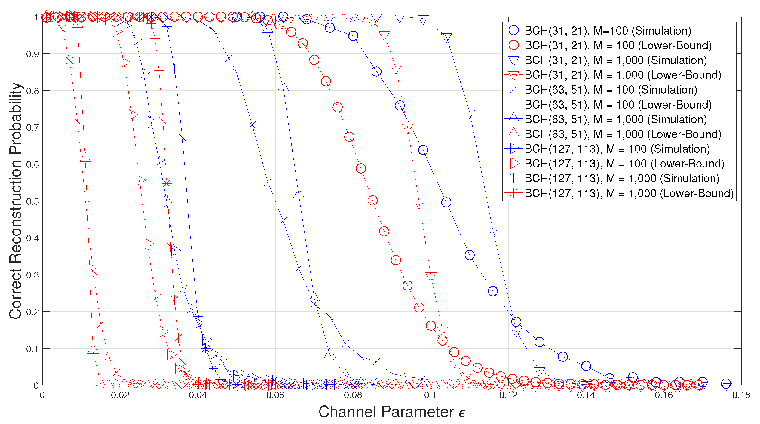
As you can see from Figure 1, the success probability of the blind reconstruction of binary BCH codes is well bounded by the lower-bound in (56). However, for $BC{H}_2(63,51)$, the gap between the simulation result and the lower-bound is larger than the others because $BC{H}_2(63,51)$ has a cyclotomic coset of cardinality 2, while all the cyclotomic cosets of $BC{H}_2(31,21)$ and $BC{H}_2(127,113)$ have the cardinality 5 and 7, respectively. In (56), if a cyclotomic coset ${\mathcal{C}}_i\subseteq {{\mathcal{C}}_{s_0}^{l_0}}^c$ has small cardinality, $1/q^{rk\left({\alpha }^i\right)}$ becomes bigger and then, $B(M,y,1/q^{rk\left({\alpha }^i\right)})$ becomes smaller. Therefore, the lower-bounds of the blind reconstruction performance of $BC{H}_2(31,21)$ and $BC{H}_2(127,113)$ is much tighter than $BC{H}_2(63,51)$.

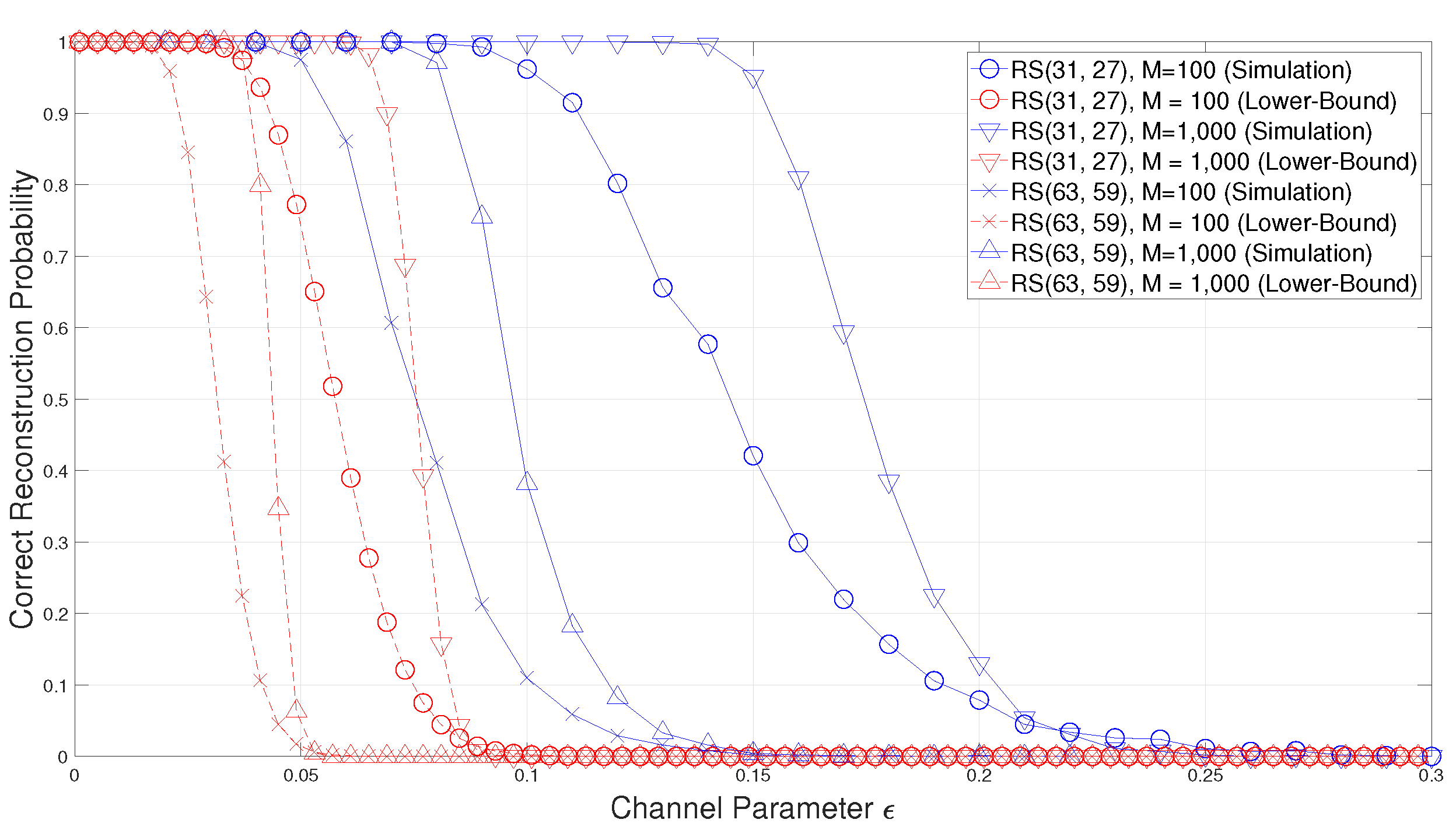
As you can see from Figure 2, the success probability of the blind reconstruction of RS codes is also well bounded by the lower-bound in (56). Moreover, as the code length increase, the proposed lower-bound of RS codes becomes tighter and therefore this lower-bound can be a good estimation of blind reconstruction performance for practical RS codes. Furthermore, since the proposed lower-bound can estimate the blind reconstruction performance without the extensive simulation, the proposed lower-bound is suitable for practical use.

5. Conclusions

The blind reconstruction method of BCH codes in [15] shows the best performance, but the theoretical analysis of this method has not been performed. In this paper, by analyzing the properties of BCH codes on the aspects of blind reconstruction, a lower-bound on the success probability of the blind reconstruction method in [15] is derived. Especially, the distribution of GFFT values of the received codewords are analyzed and the blind reconstruction method is formalized based on the conjugacy classes. Furthermore, the analysis results can be applied not only to the binary BCH codes, but also to the non-binary BCH codes, including RS codes. By comparing the derived lower-bound with the simulation results, it is confirmed that the success probability of the blind reconstruction is well bounded by the proposed lower-bound.

References

- Wicker, S. Error control coding for digital communication systems In Error Control Systems for Digital Communication and Storage; Prentice-Hall: Englewood Cliffs, NJ, USA, 1995; pp. 1–16. [Google Scholar]
- Valembois, A. Detection and recognition of a binary linear code. Discret. Appl. Math. 2001, 111, 199–218. [Google Scholar] [CrossRef]
- Cluzeau, M. Block code reconstruction using iterative decoding techniques. In Proceedings of the 2006 IEEE International Symposium on Information Theory (ISIT 2006), Seattle, DC, USA, 9–14 July 2006; pp. 2269–2273. [Google Scholar]
- Burel, G.; Gautier, R. Blind estimation of encoder and interleaver characteristics in a non cooperative context. In Proceedings of the IASTED International Conference on Communications, Internet and Information Technology (CIIT 2003), Scottsdale, AZ, USA, 17–19 November 2003. [Google Scholar]
- Moosavi, R.; Larsson, E. Fast blind recognition of channel codes. IEEE Trans. Commun. 2014, 62, 1393–1405. [Google Scholar] [CrossRef] [Green Version]
- Chabot, C. Recognition of a code in a noisy environment. In Proceedings of the 2007 IEEE International Symposium on Information Theory (ISIT 2007), Nice, France, 24–29 June 2007; pp. 2211–2215. [Google Scholar]
- Yardi, A.; Kumar, A.; Vijayakumaran, S. Channel-code detection by a third-party receiver via the likelihood ratio test. In Proceedings of the 2014 IEEE International Symposium on Information Theory (ISIT 2014), Honolulu, HI, USA, 24 June–4 July 2014; pp. 1051–1055. [Google Scholar]
- Yardi, A.; Vijayakumaran, S.; Kumar, A. Blind reconstruction of binary cyclic codes. In Proceedings of the 20th European Wireless Conference, Barcelona, Spain, 14–16 May 2014; pp. 849–854. [Google Scholar]
- Yardi, A.; Vijayakumaran, S.; Kumar, A. Blind reconstruction of binary cyclic codes from unsynchronized bitstream. IEEE Trans. Commun. 2016, 64, 2693–2706. [Google Scholar] [CrossRef]
- Wu, G.; Zhang, B.; Wen, X.; Guo, D. Blind recognition of BCH code based on Galois field Fourier transform. In Proceedings of the 2015 International Conference on Wireless Communications and Signal Processing (WCSP), Nanjing, China, 15–17 October 2015; pp. 1–4. [Google Scholar]
- Wang, J.; Yue, Y.; Yao, J. Statistical recognition method of binary BCH code. Commun. Netw. 2011, 3, 17–22. [Google Scholar] [CrossRef] [Green Version]
- Jing, Z.; Zhiping, H. Blind recognition of binary BCH codes for cognitive radios. Math. Probl. Eng. 2016, 2016, 1–6. [Google Scholar]
- Lee, H.; Park, C.; Lee, J.; Song, Y. Reconstruction of BCH codes using probability compensation. In Proceedings of the 18th Asia-Pacific Conference on Communications (APCC), Jeju, Korea, 15–17 October 2012; pp. 591–594. [Google Scholar]
- Li, C.; Zhang, T.; Lin, Y. Blind recognition of RS codes based on Galois field columns Gaussian elimination. In Proceedings of the 7th International Congress on Image and Signal Processing, Dalian, China, 14–16 October 2014; pp. 836–841. [Google Scholar]
- Jo, D.; Kwon, S.; Shin, D. Blind reconstruction of BCH codes based on consecutive roots of generator polynomials. IEEE Commun. Lett. 2018, 22, 894–897. [Google Scholar] [CrossRef]
- Filiol, E. Reconstruction of convolutional encoders over GF(q). In IMA International Conference on Cryptography and Coding; Springer: Berlin/Heidelberg, Germany, 1997; Volume 1355, pp. 101–109. [Google Scholar] [CrossRef]
- Lu, P.; Li, S.; Luo, X.; Zou, Y. Blind recognition of punctured convolutional codes. In Proceedings of the 2004 International Symposium on Information Theory (ISIT 2004), Chicago, IL, USA, 27 June–2 July 2004; p. 457. [Google Scholar]
- Barbier, J. Reconstruction of turbo-code encoder. In Digital Wireless Communications VII and Space Communication Technologies; International Society for Optics and Photonics: Bellingham, WA, USA, 2005; pp. 463–473. [Google Scholar]
- Marazin, M.; Gautier, R.; Burel, G. Blind recovery of k/n rate convolutional encoders in a noisy environment. EURASIP J. Wirel. Commun. Netw. 2011, 2011, 1–9. [Google Scholar] [CrossRef]
- Yardi, A. Blind reconstruction of binary cyclic codes over binary erasure channel. In Proceedings of the 2018 International Symposium on Information Theory and Its Applications (ISITA), Singapore, 28–31 October 2018; pp. 301–305. [Google Scholar]
Figure 1.
Comparison of the correct reconstruction probability with the proposed lower-bound for binary Bose–Chaudhuri–Hocquenghem (BCH) codes.
Figure 2.
Comparison of the correct reconstruction probability with the proposed lower-bound for Reed–Solomon (RS) codes.
Publisher’s Note: MDPI stays neutral with regard to jurisdictional claims in published maps and institutional affiliations. |
© 2020 by the authors. Licensee MDPI, Basel, Switzerland. This article is an open access article distributed under the terms and conditions of the Creative Commons Attribution (CC BY) license (http://creativecommons.org/licenses/by/4.0/).
Share and Cite
MDPI and ACS Style
Kwon, S.; Shin, D.-J. Analysis of Blind Reconstruction of BCH Codes. Entropy 2020, 22, 1256. https://doi.org/10.3390/e22111256
AMA Style
Kwon S, Shin D-J. Analysis of Blind Reconstruction of BCH Codes. Entropy. 2020; 22(11):1256. https://doi.org/10.3390/e22111256
Chicago/Turabian StyleKwon, Soonhee, and Dong-Joon Shin. 2020. "Analysis of Blind Reconstruction of BCH Codes" Entropy 22, no. 11: 1256. https://doi.org/10.3390/e22111256
Note that from the first issue of 2016, this journal uses article numbers instead of page numbers. See further details here.