Entropy Generation in MHD Mixed Convection Non-Newtonian Second-Grade Nanoliquid Thin Film Flow through a Porous Medium with Chemical Reaction and Stratification

 ,
,  , , , and
Abstract
:1. Introduction
2. Methods
Basic Equations
3. Entropy Generation
4. Analytical Solution of the Problem by Homotopy Analysis Method
4.1. Zeroth-Order Deformation Problems
4.2. m-th Order Deformation Problems
5. Results
6. Discussion
6.1. Velocity Profile
6.2. Temperature Profile
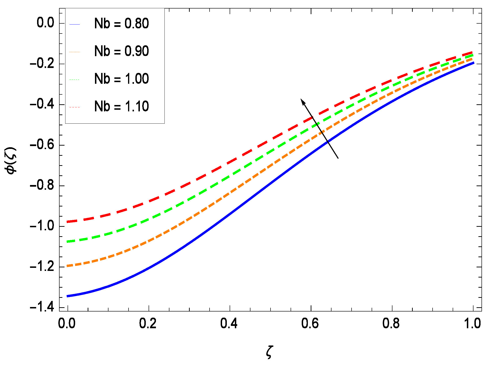
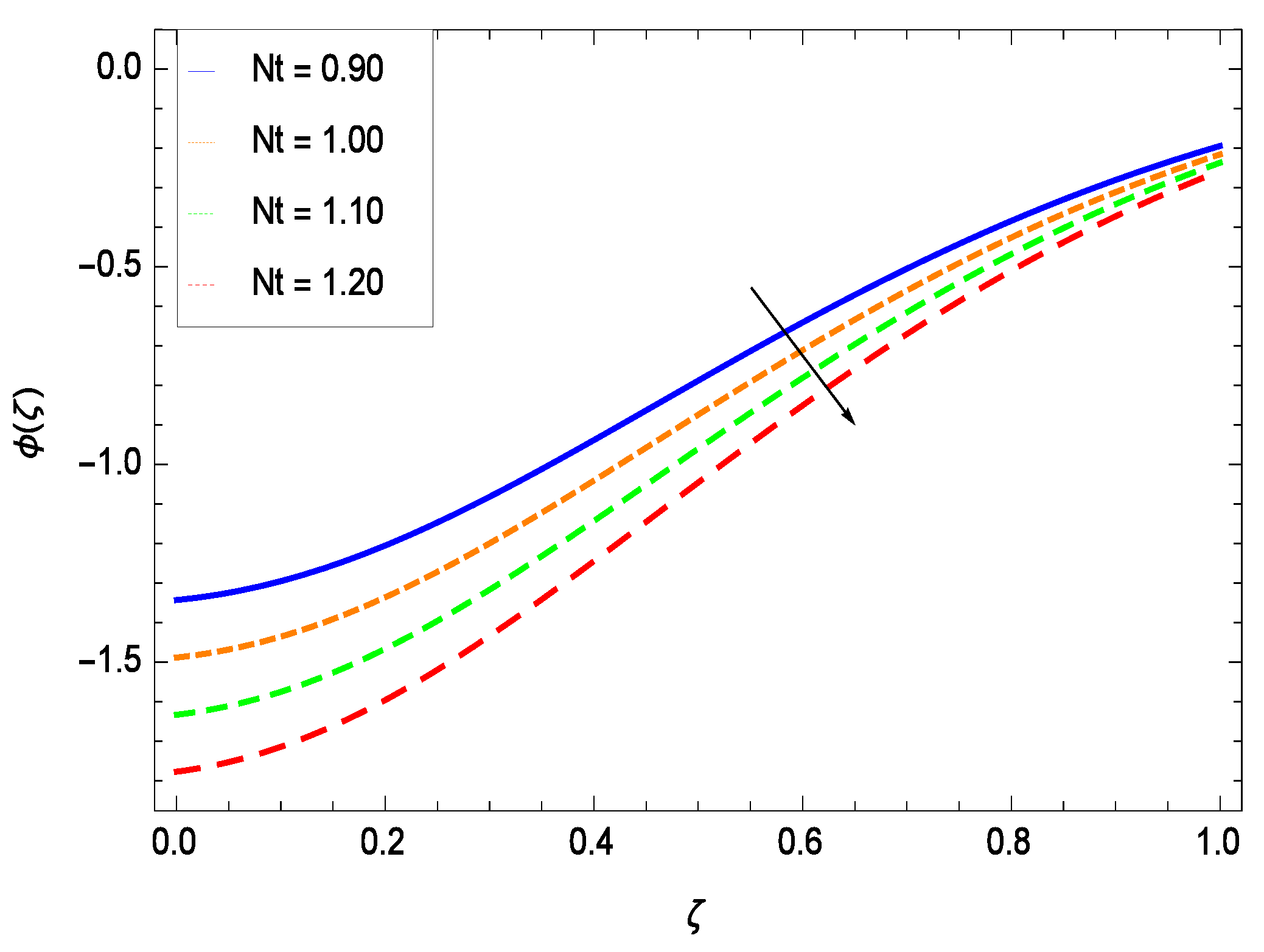
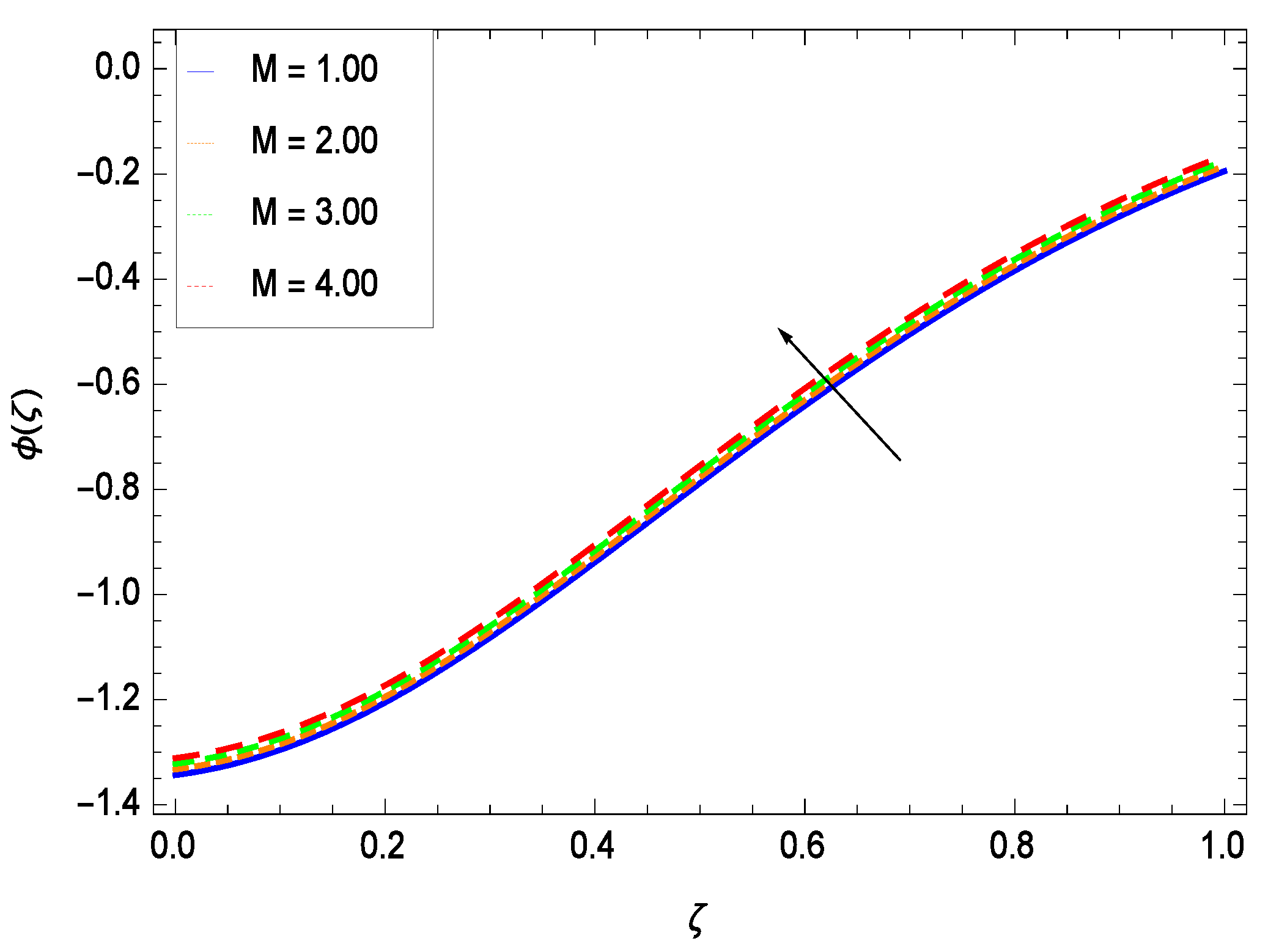
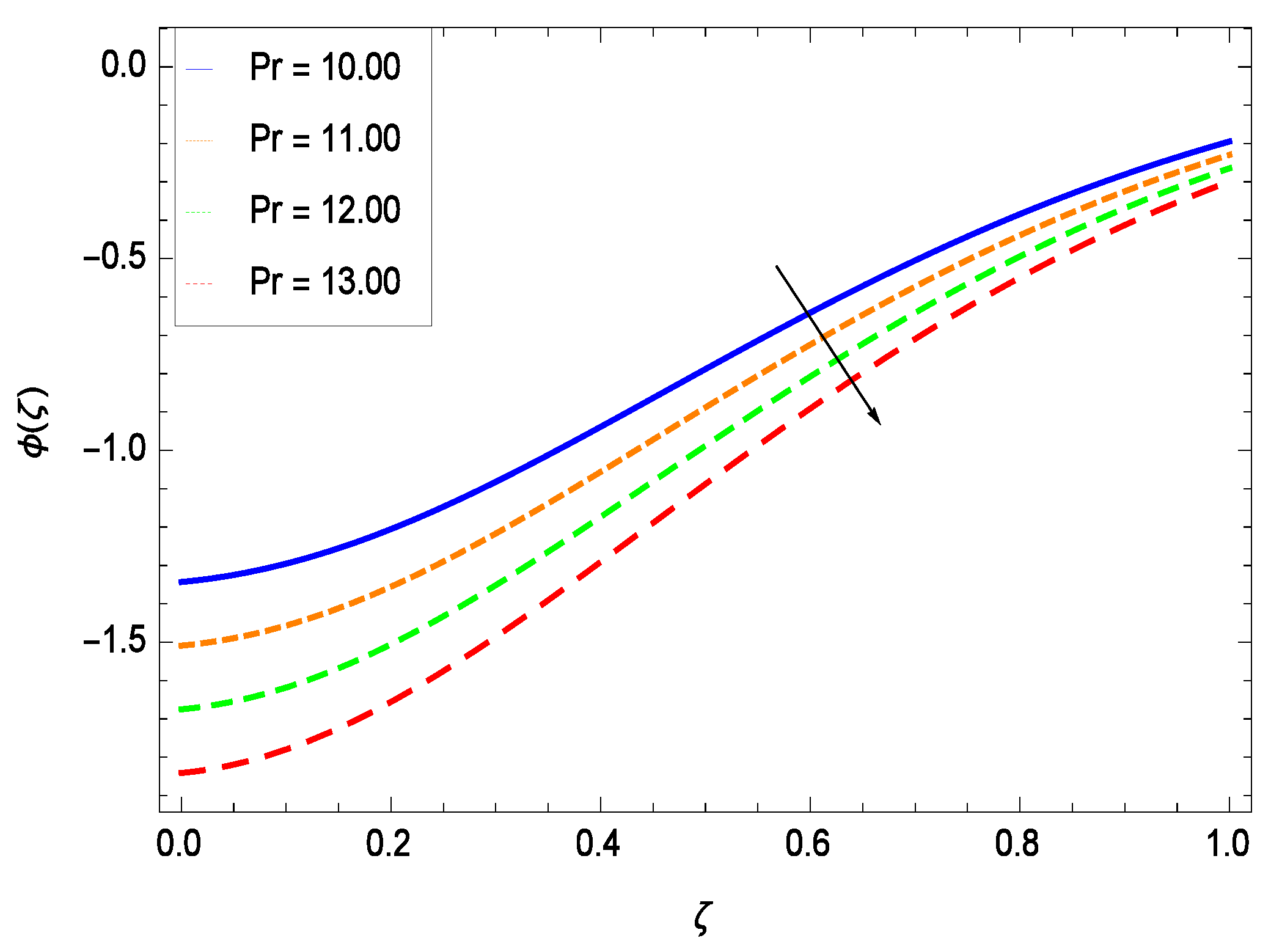
6.3. Nanoparticle Concentration Profile
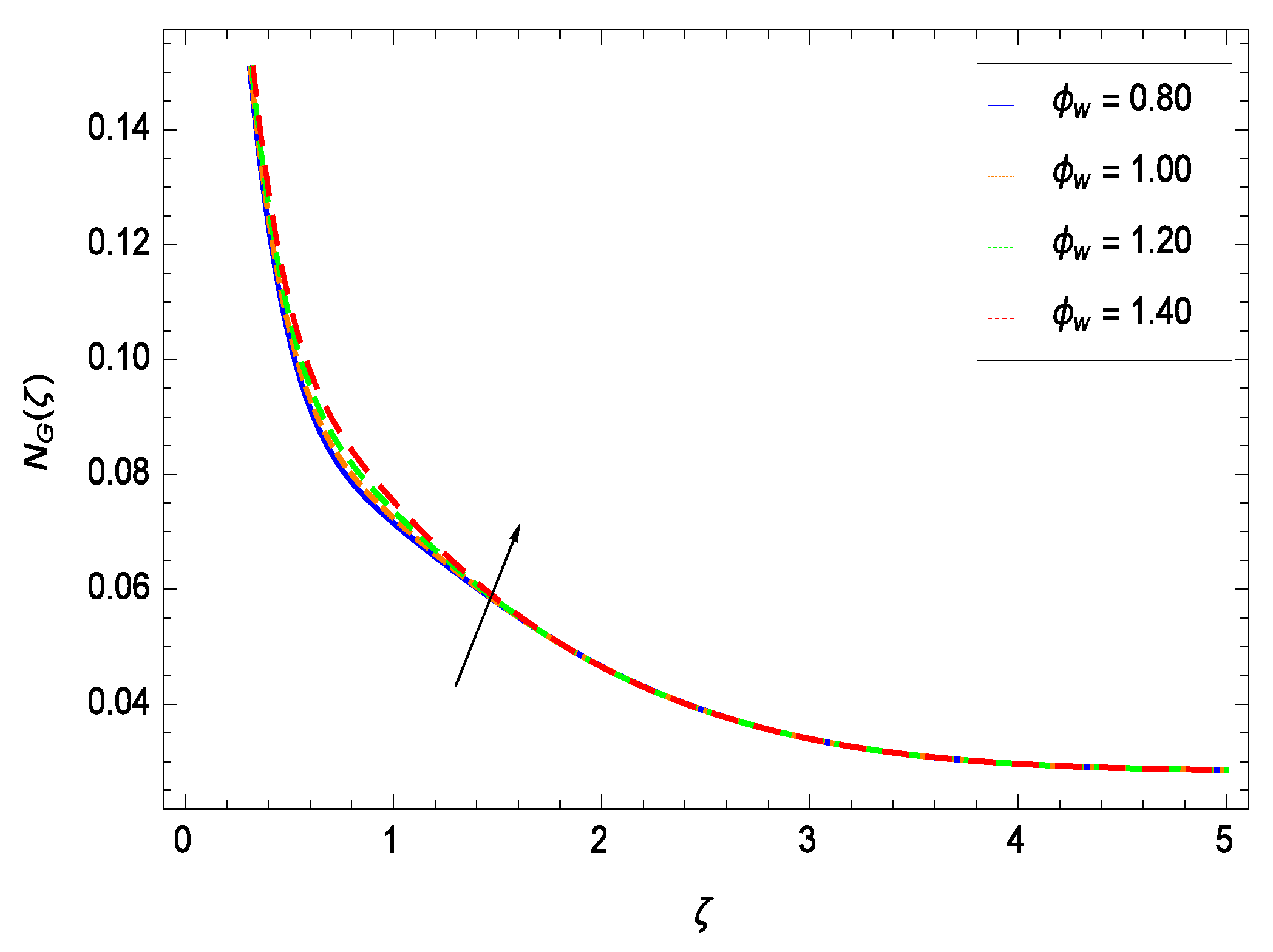
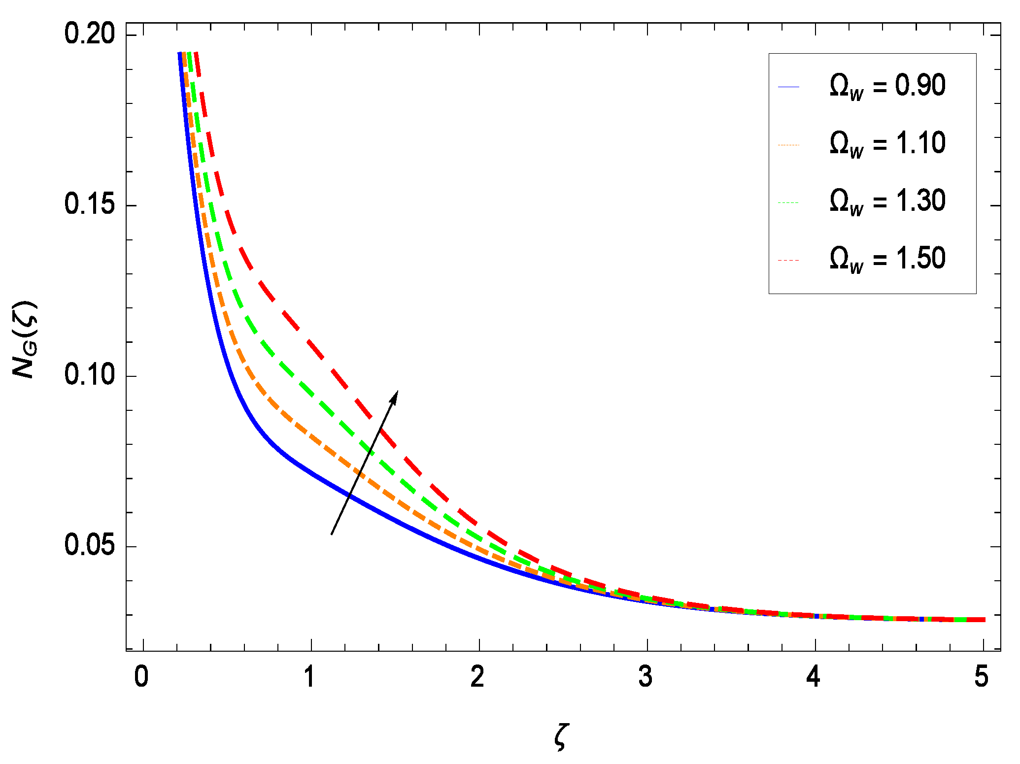
6.4. Gyrotactic Microorganism Concentration
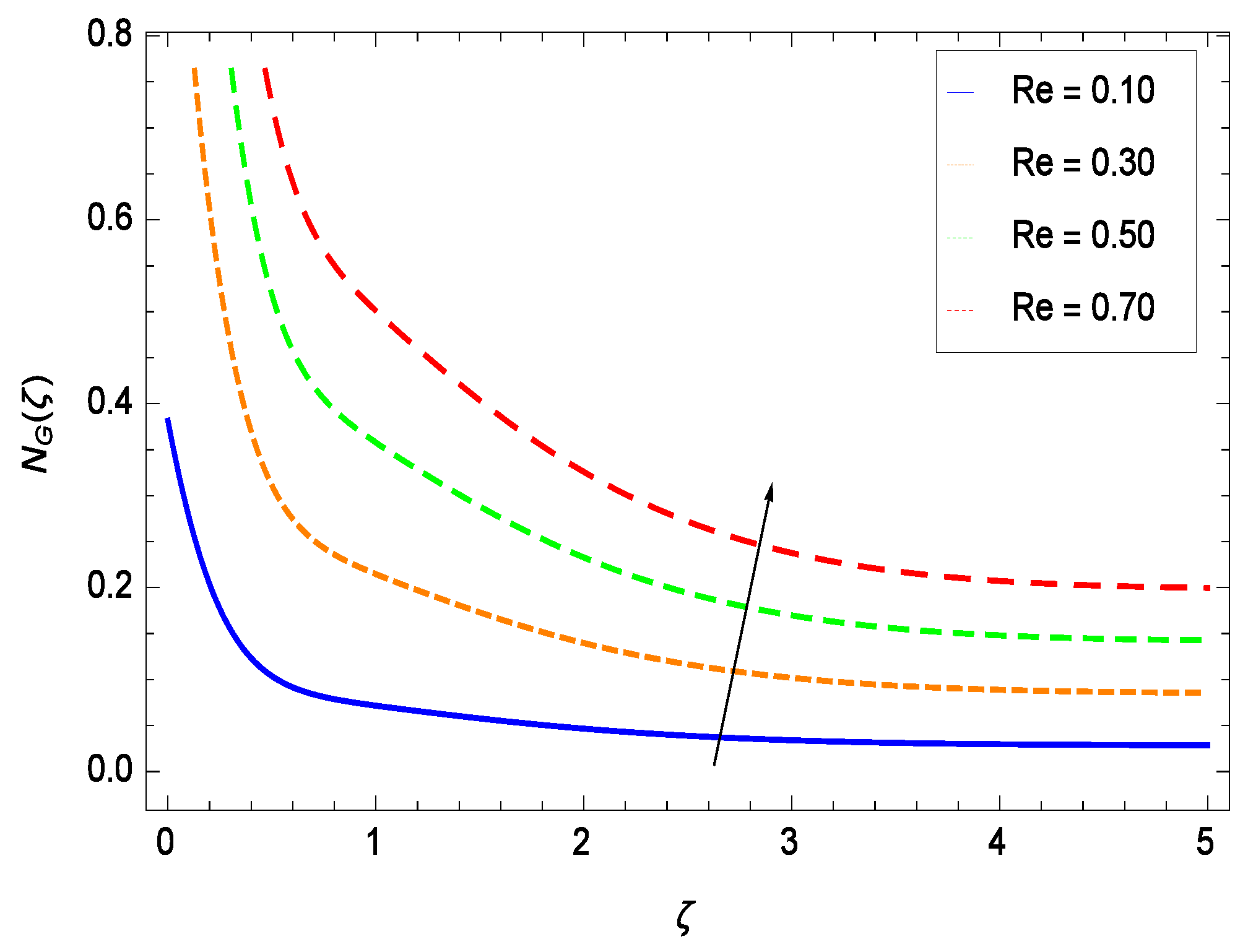
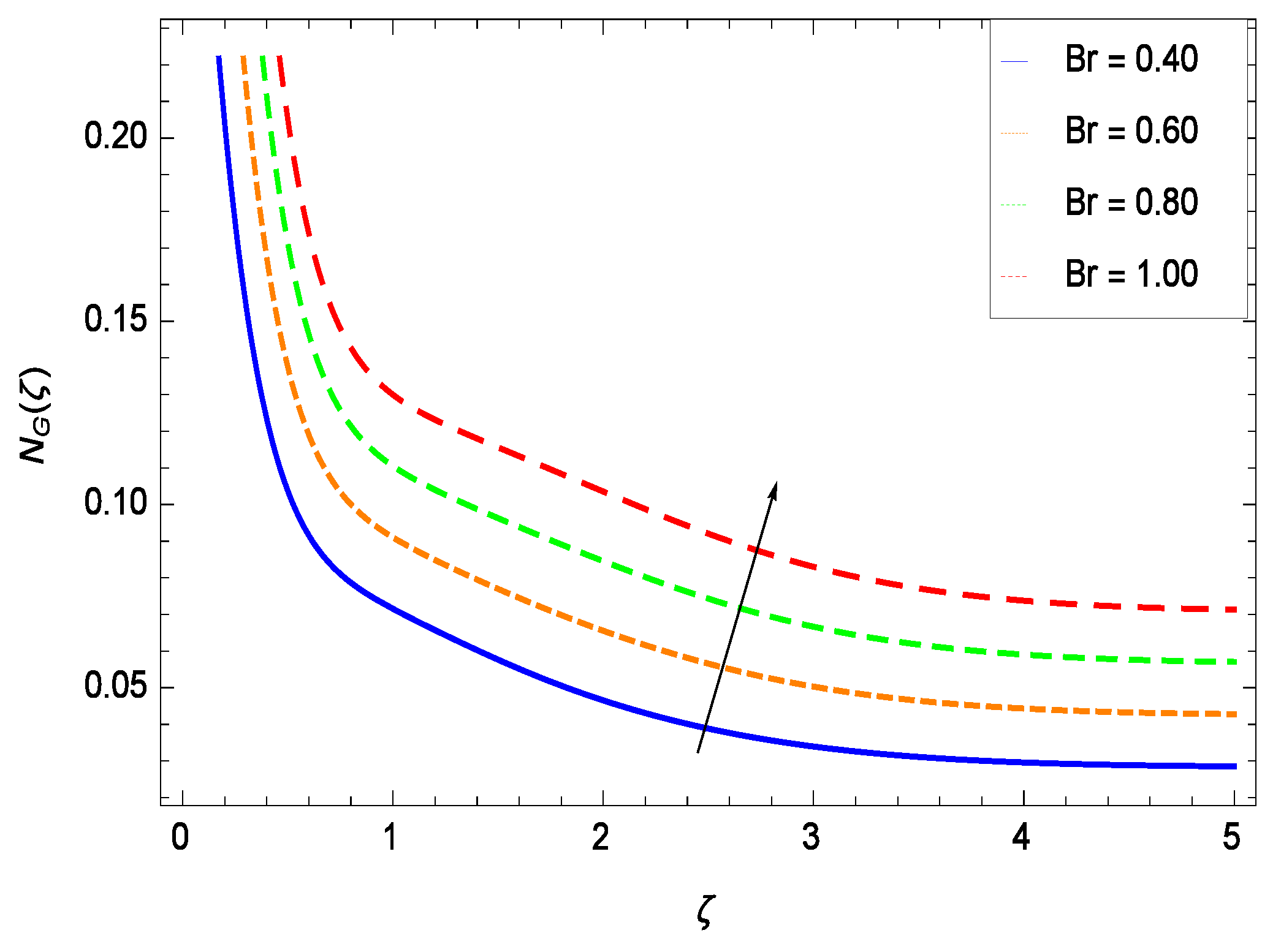
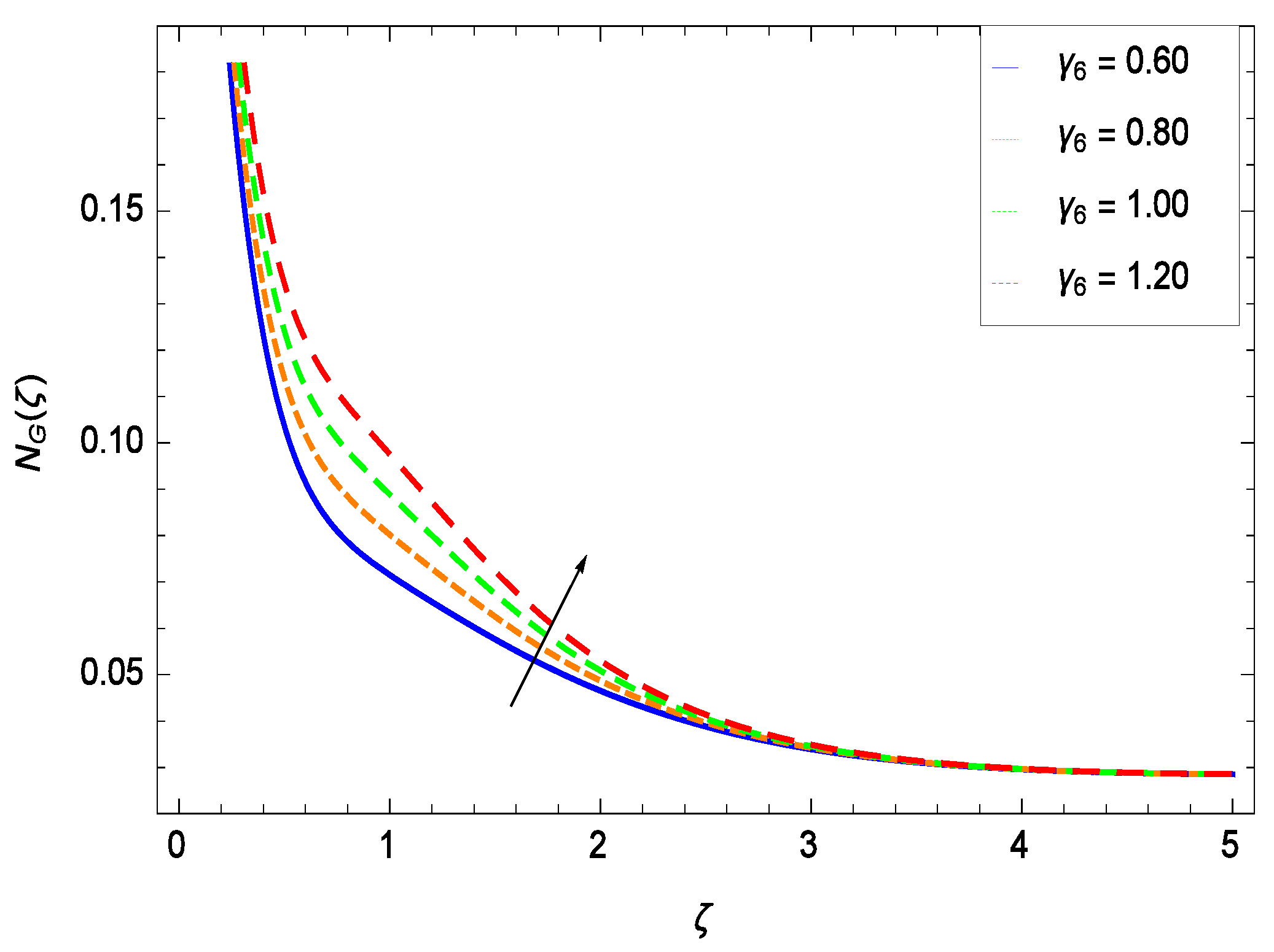
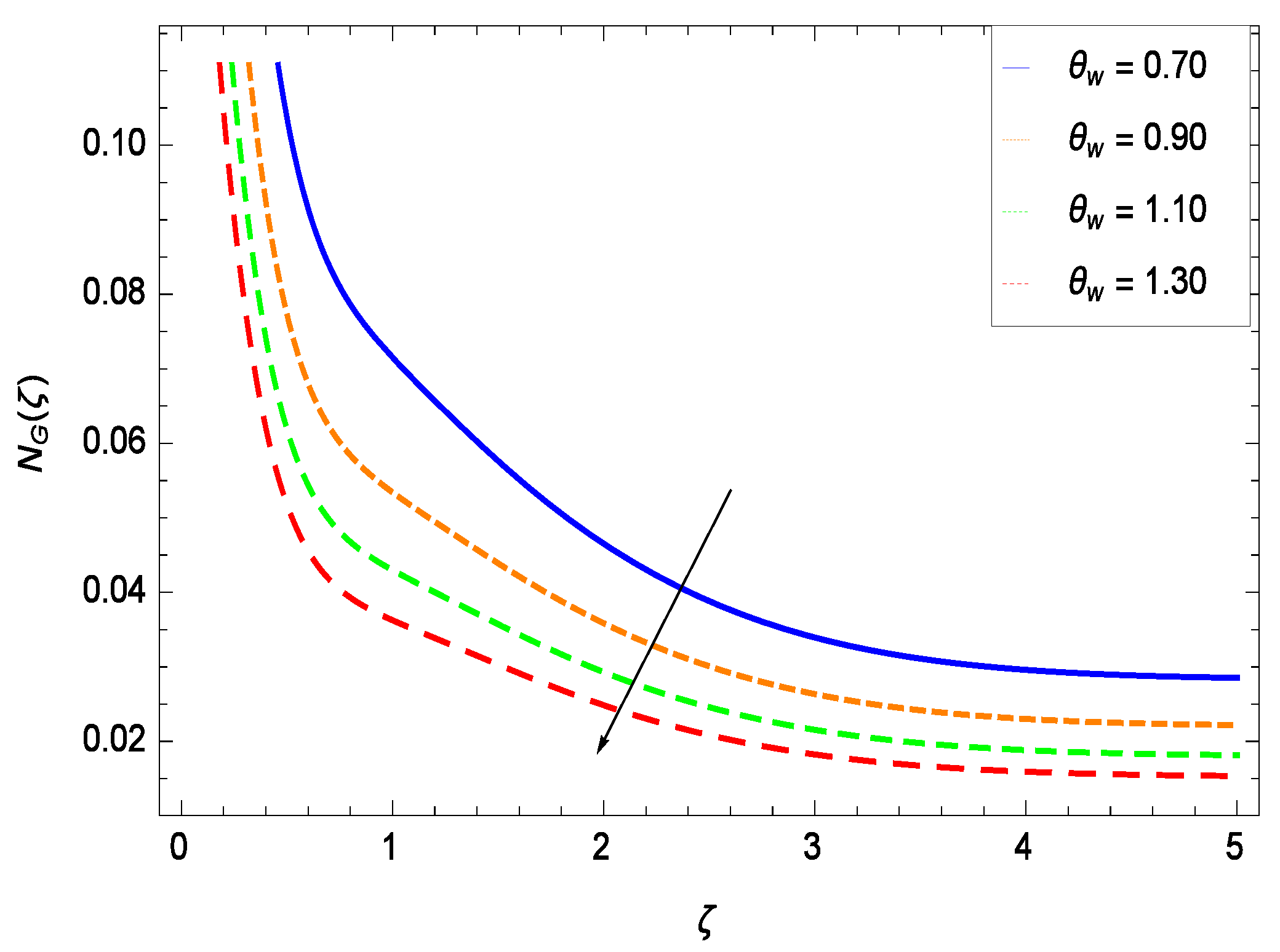
7. Entropy Generation Analysis
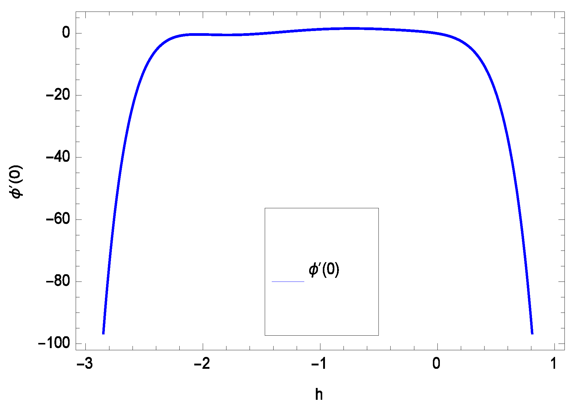
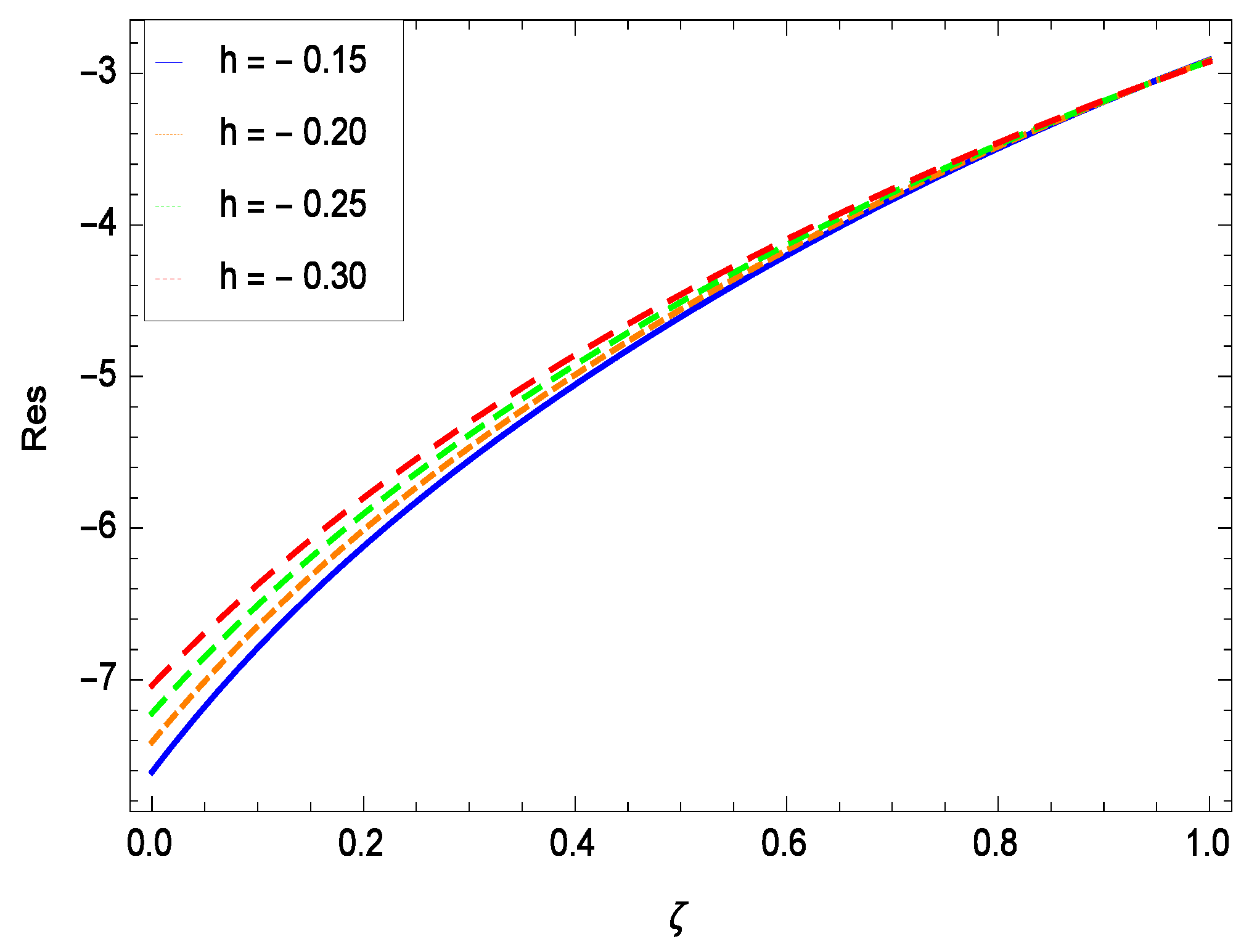
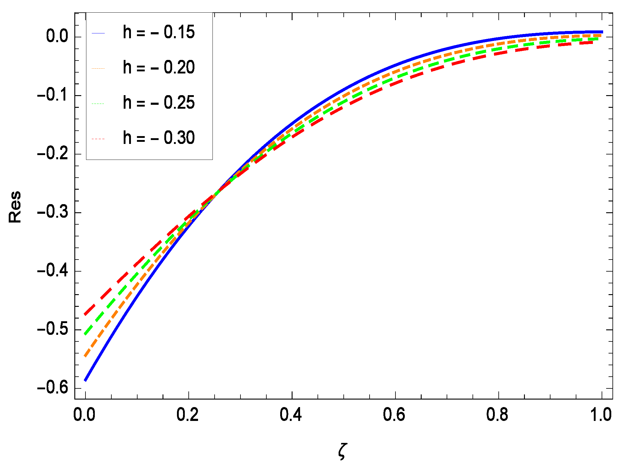
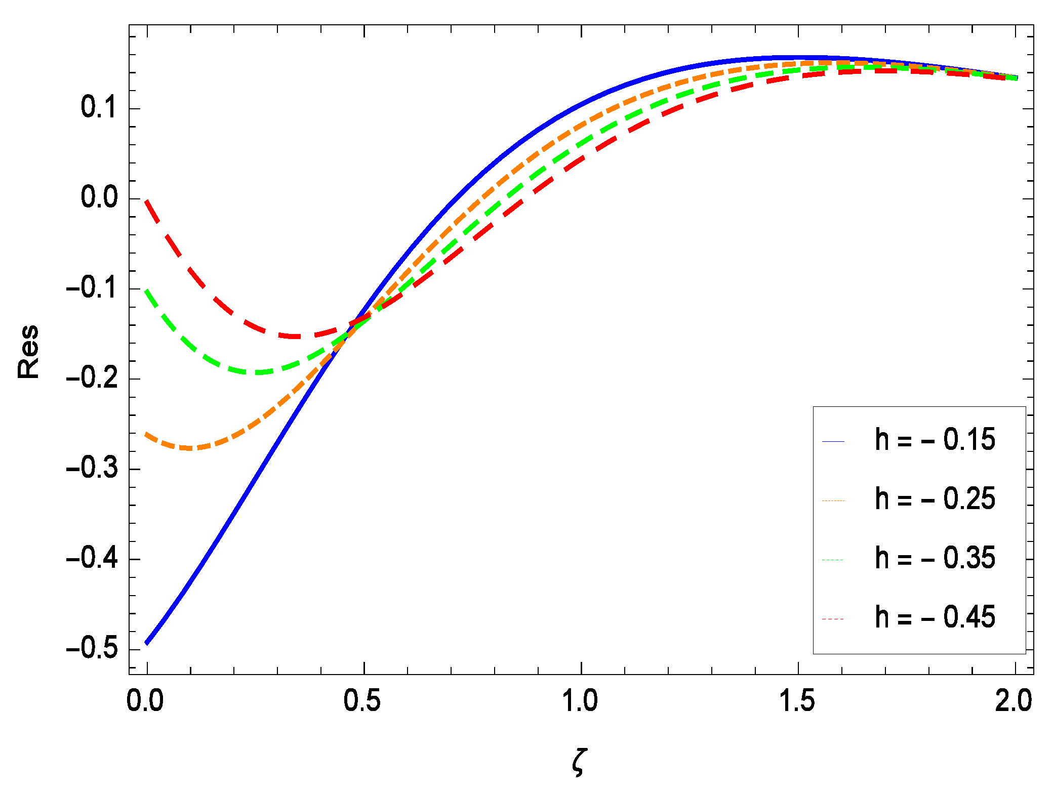
8. Residual Errors
9. Conclusions
- (i)
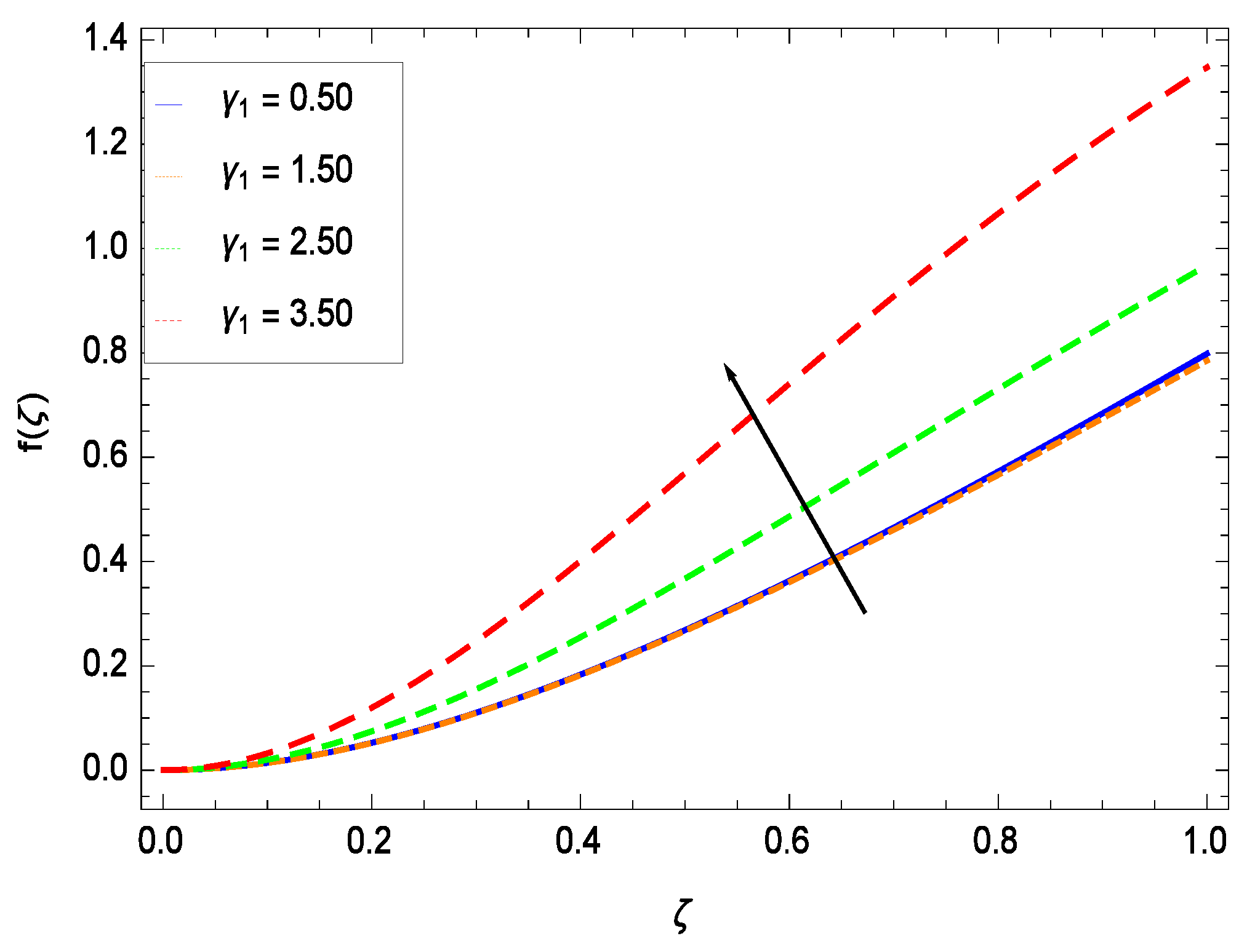
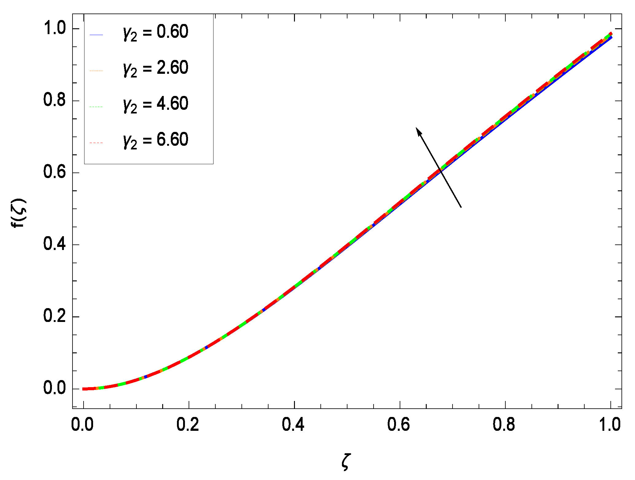
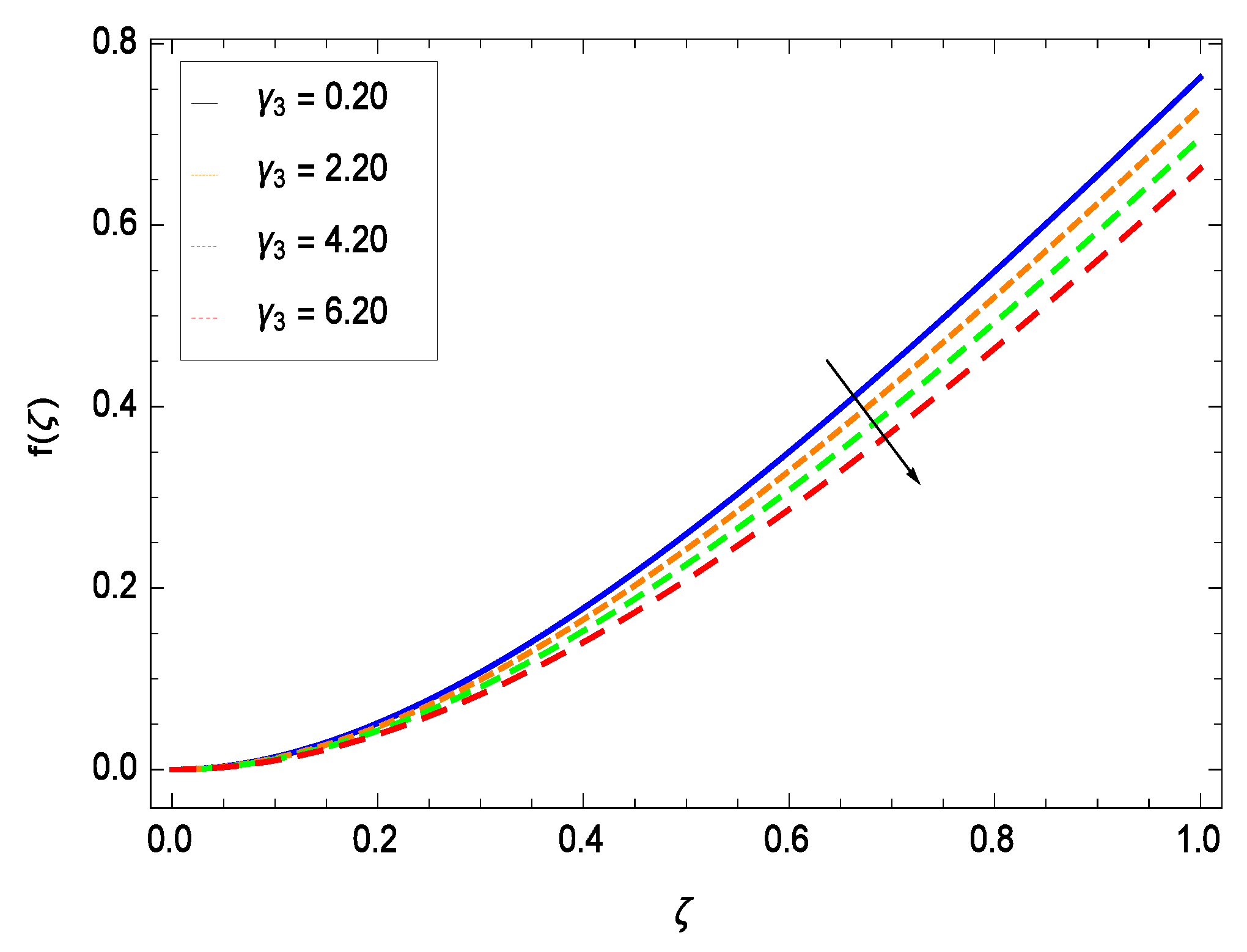
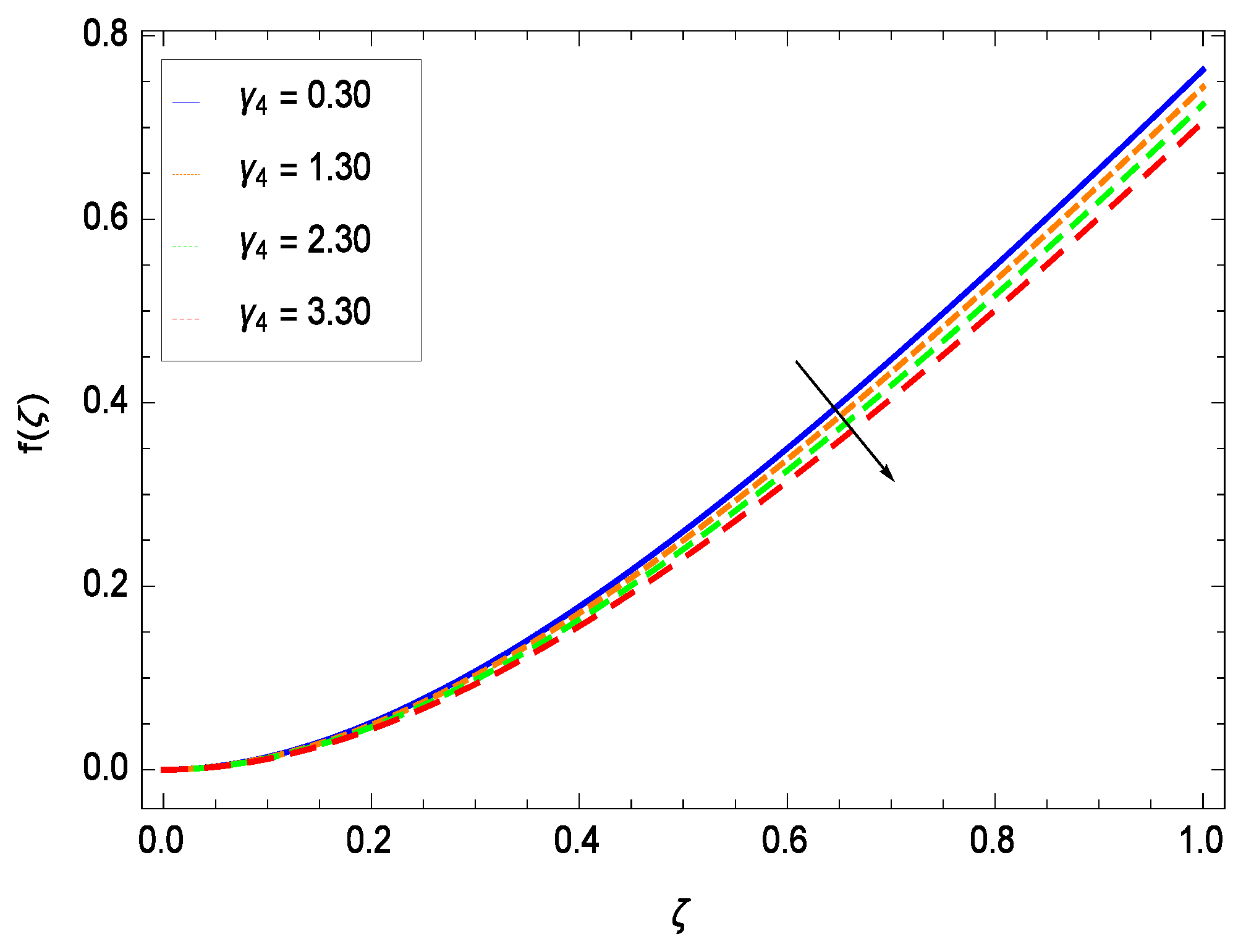
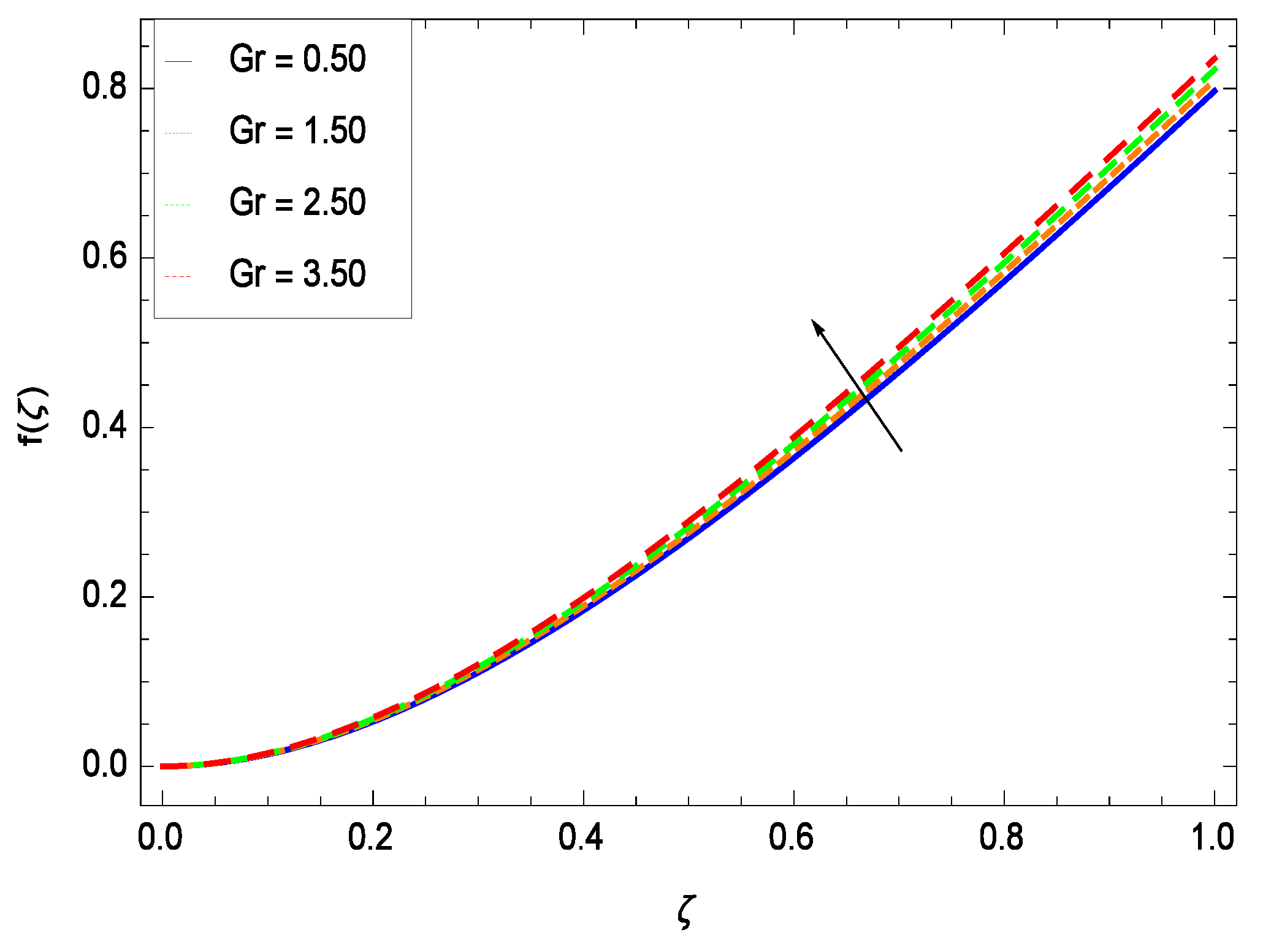
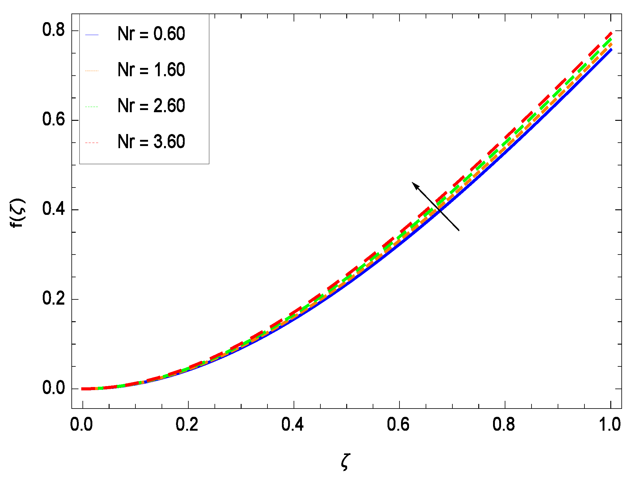
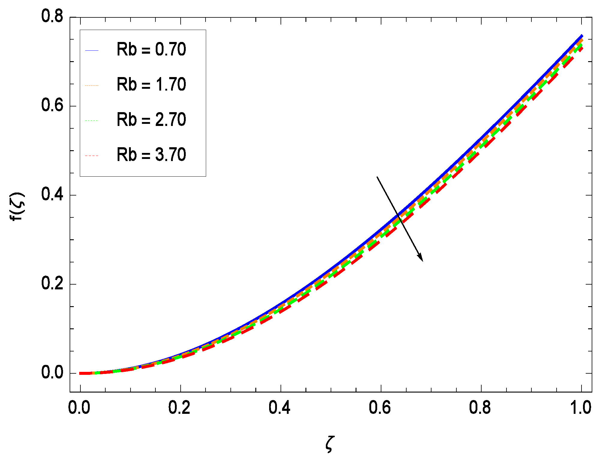
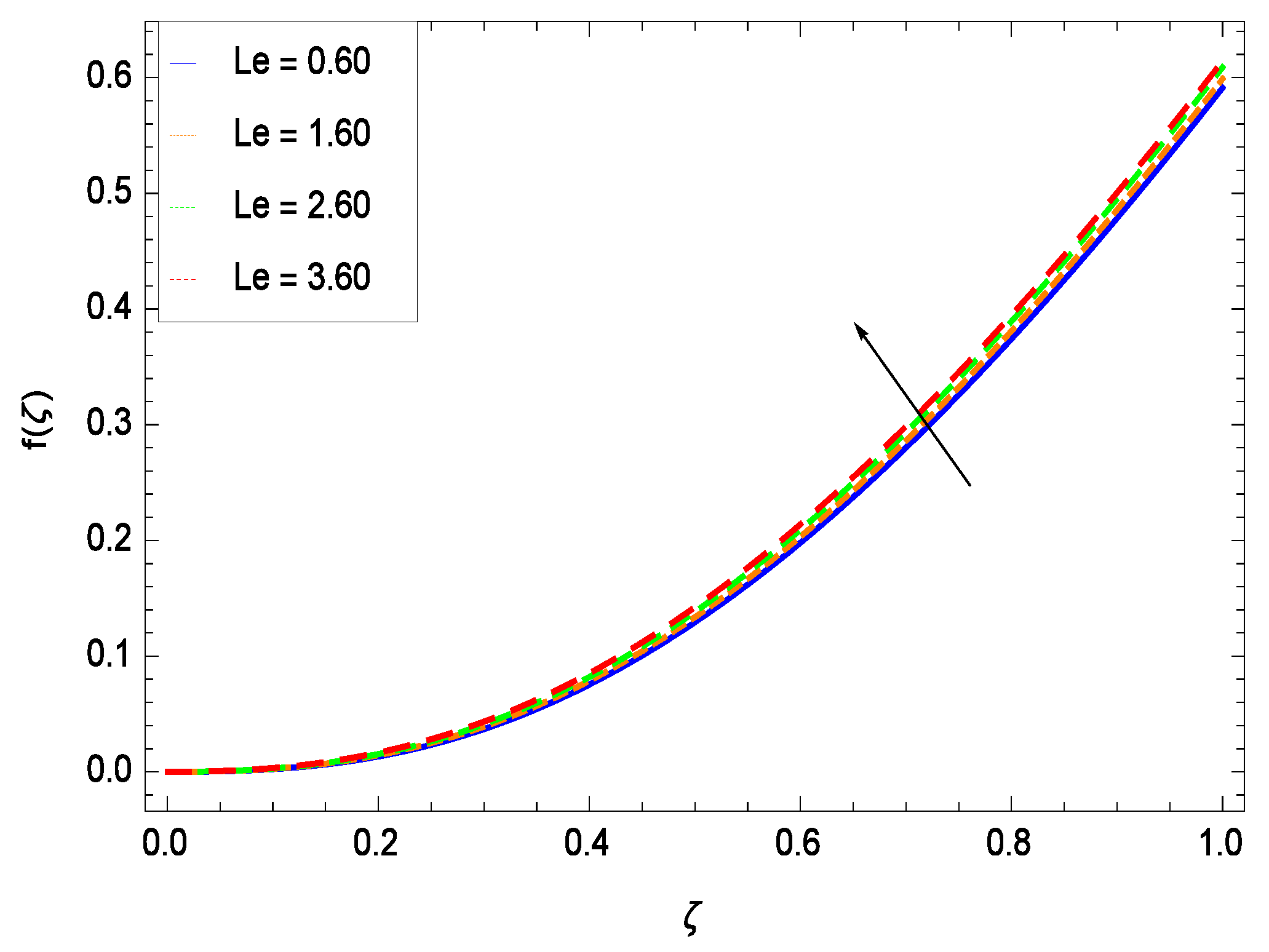
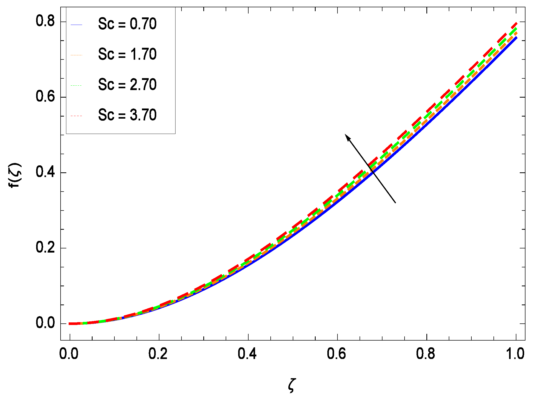
- The velocity f() depreciates for the porosity parameter , inertial parameter , bioconvection Rayleigh number Rb and magnetic field parameter M while it elevates for the second grade nanofluid parameter , reduced heat transfer parameter , chemical reaction parameter , buoyancy parameter Gr, buoyancy ratio parameter Nr, Lewis number Le, Schmidt number Sc and Prandtl number Pr.
- (ii)
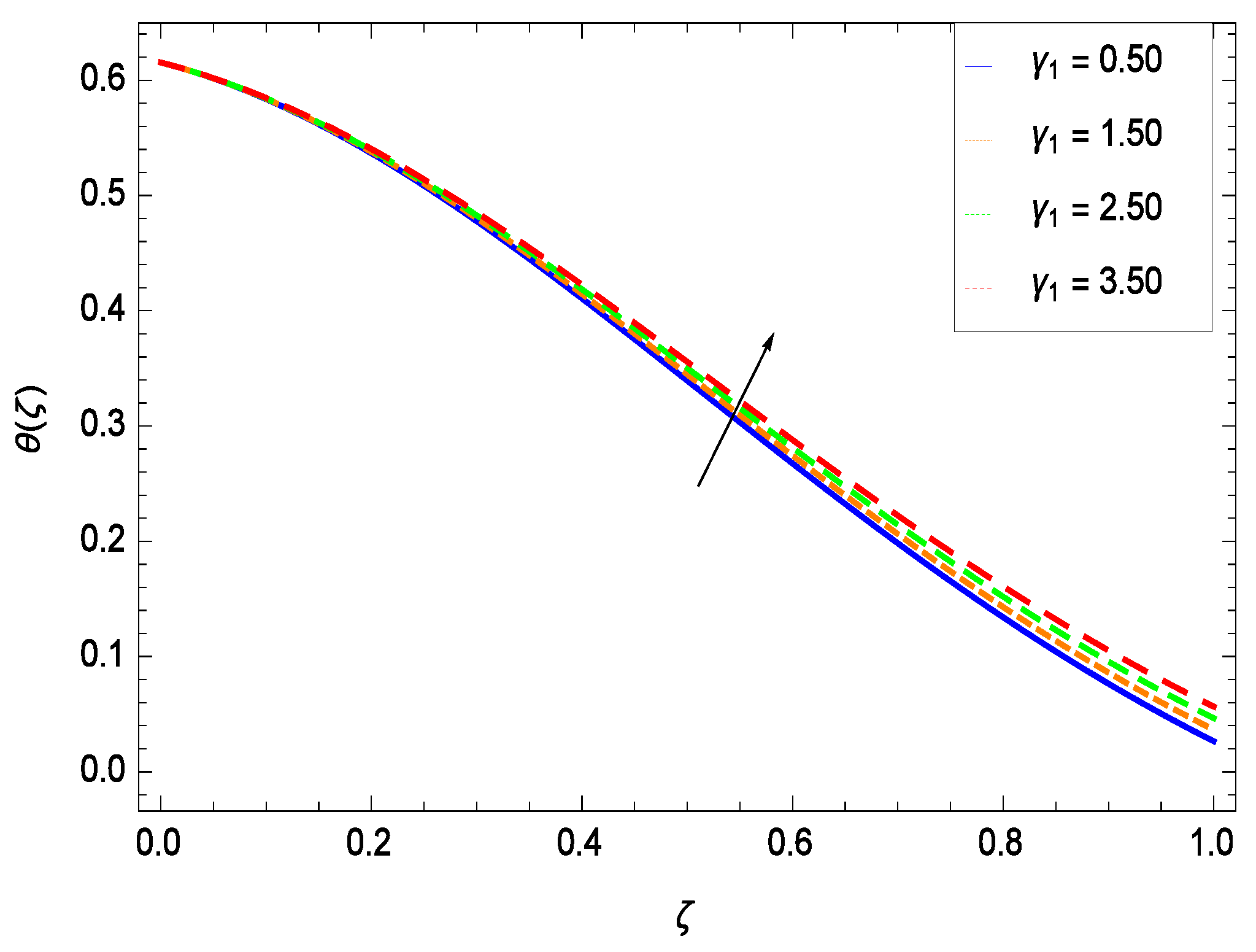
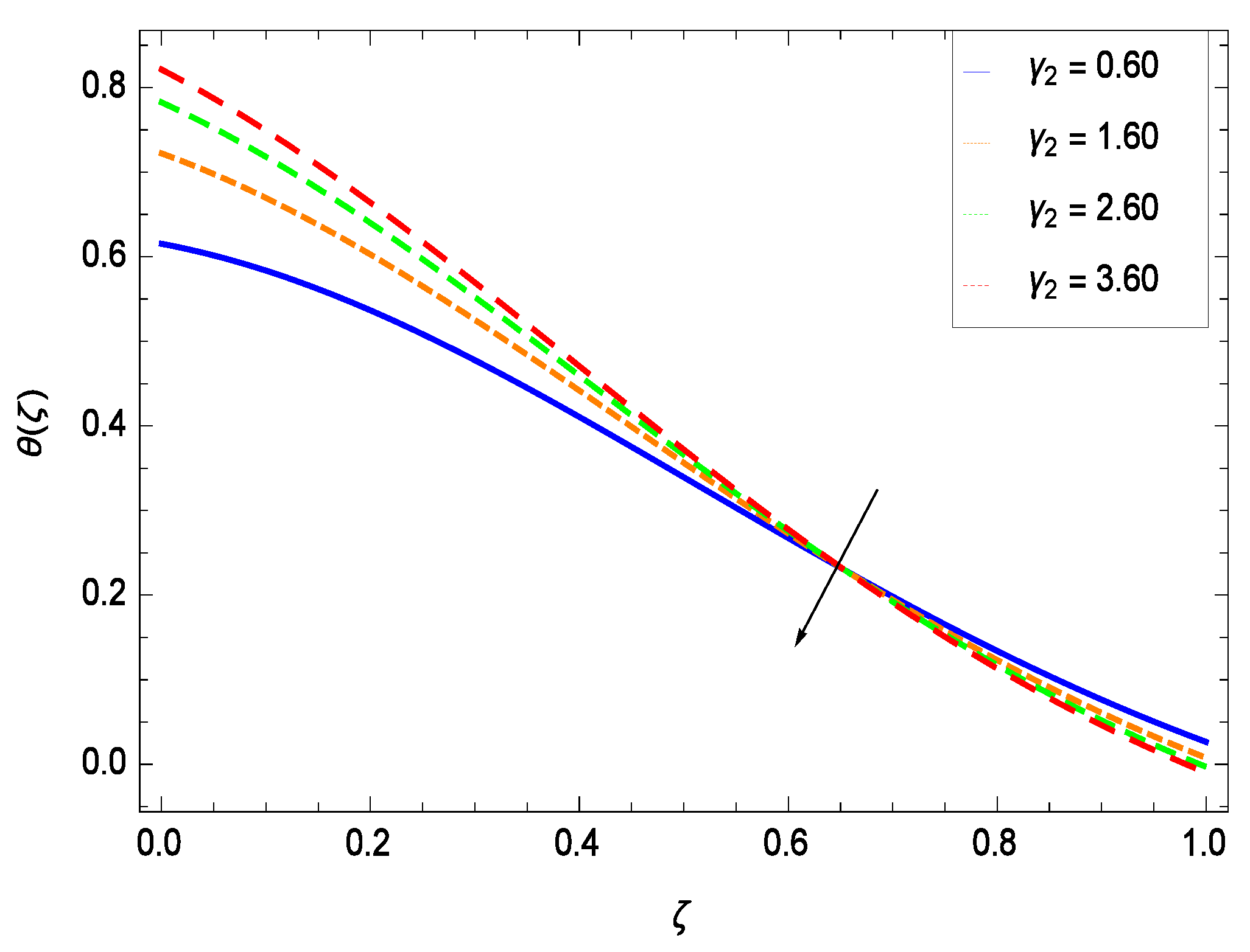
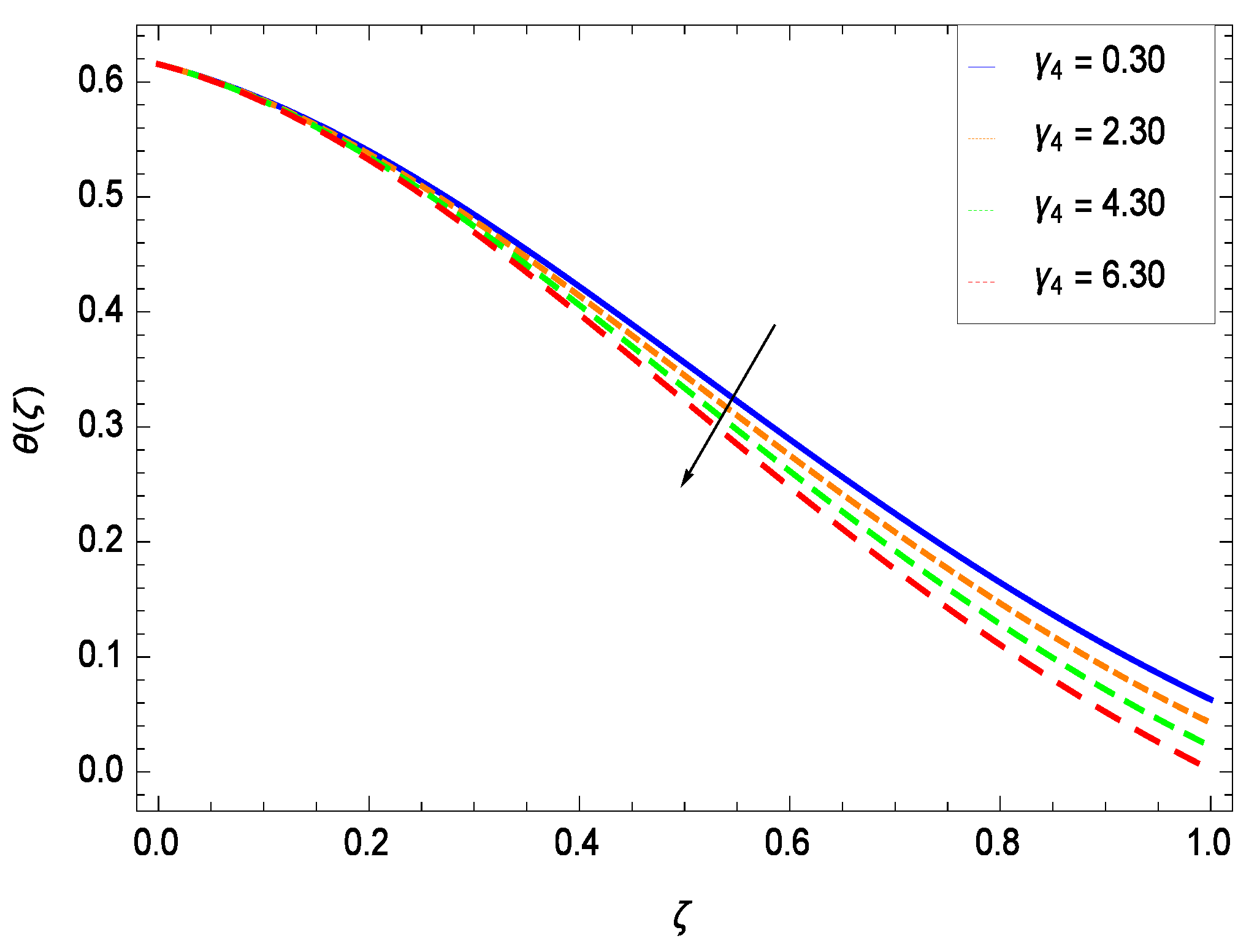
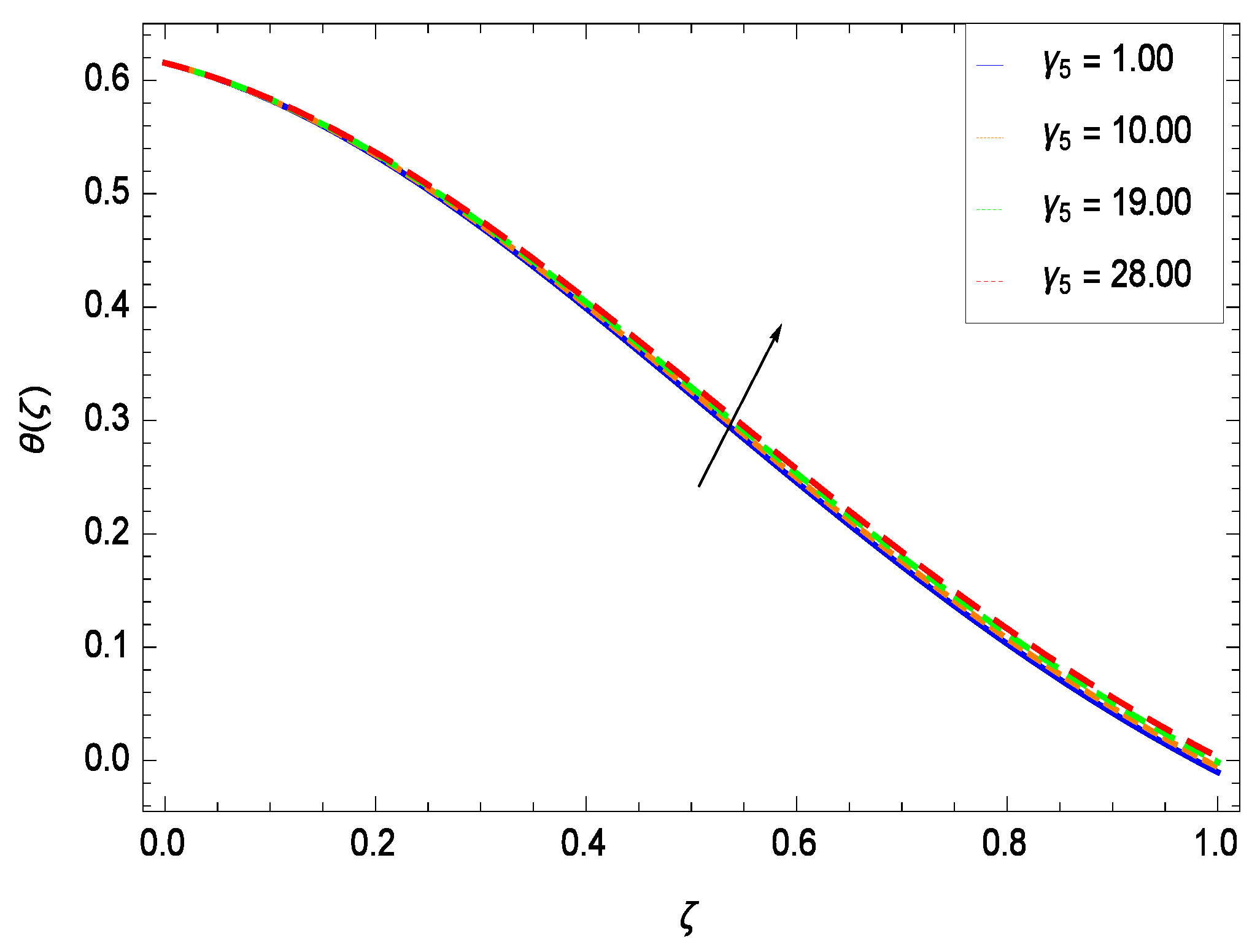
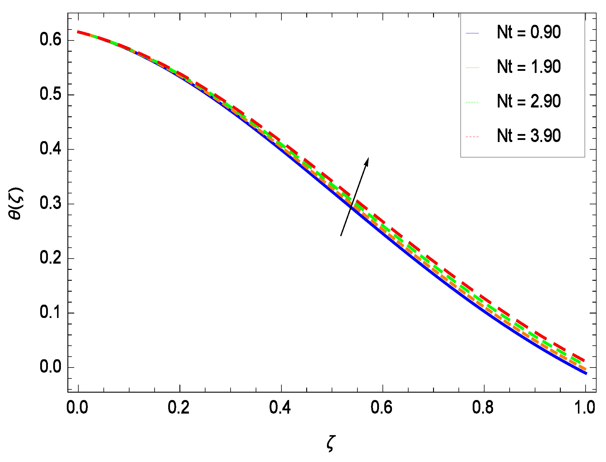
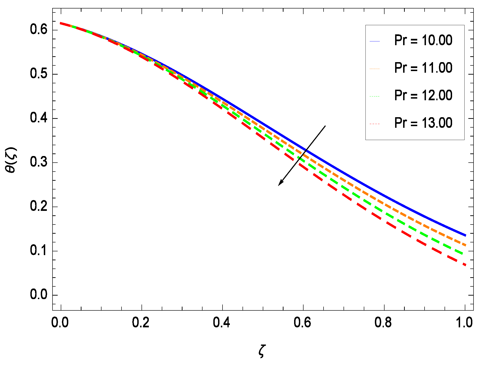
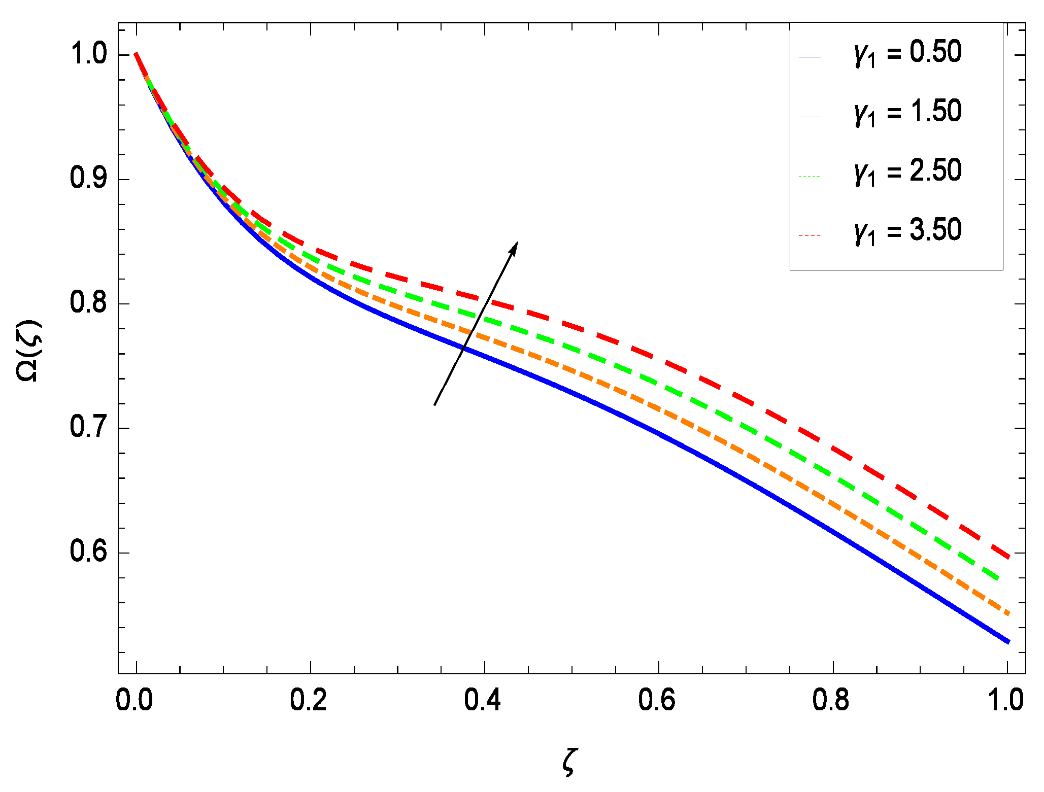
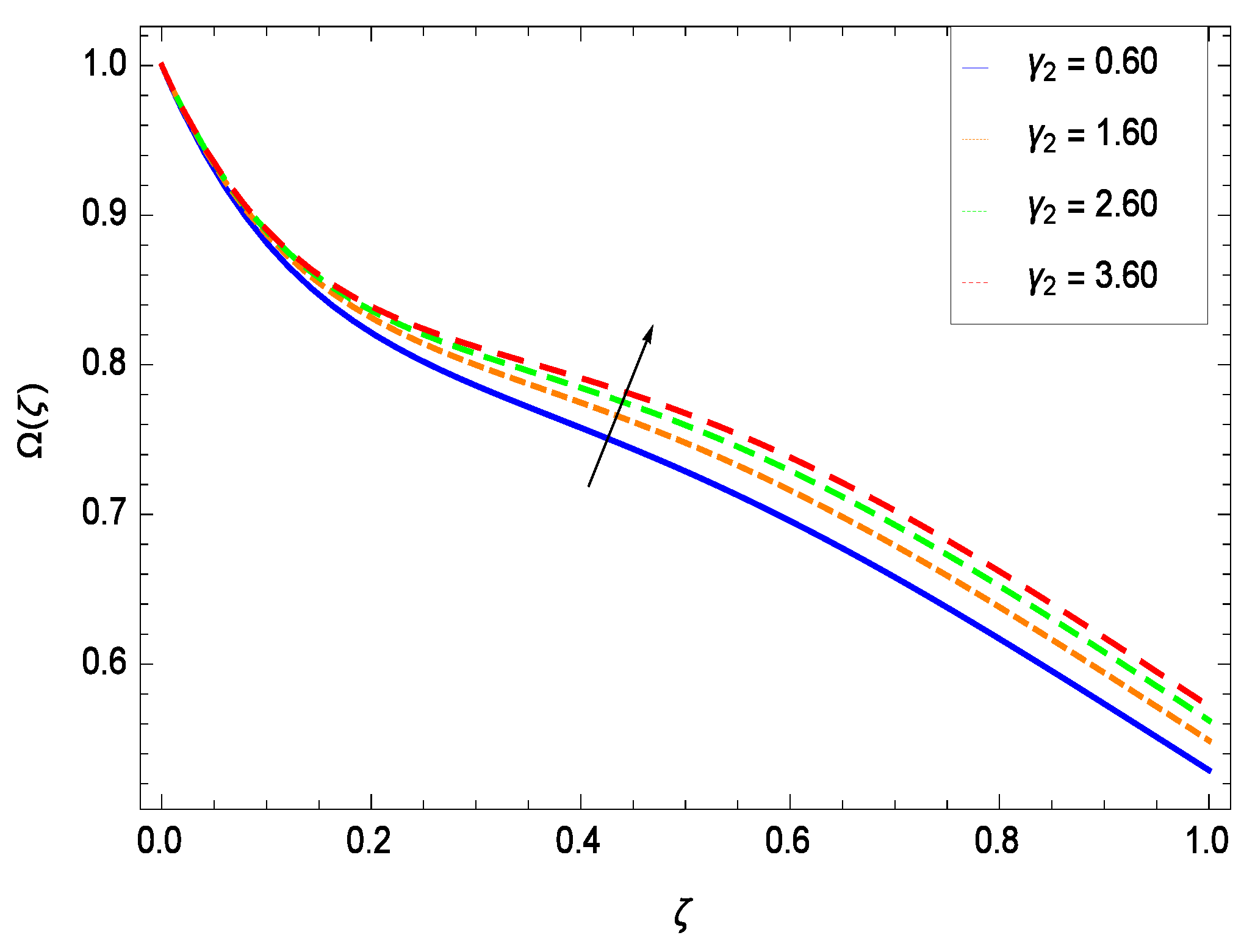
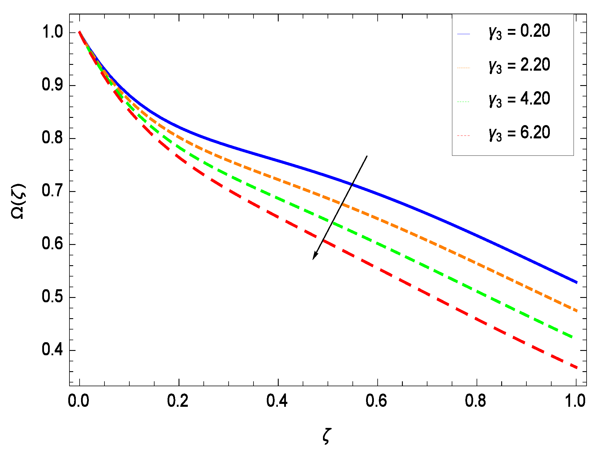
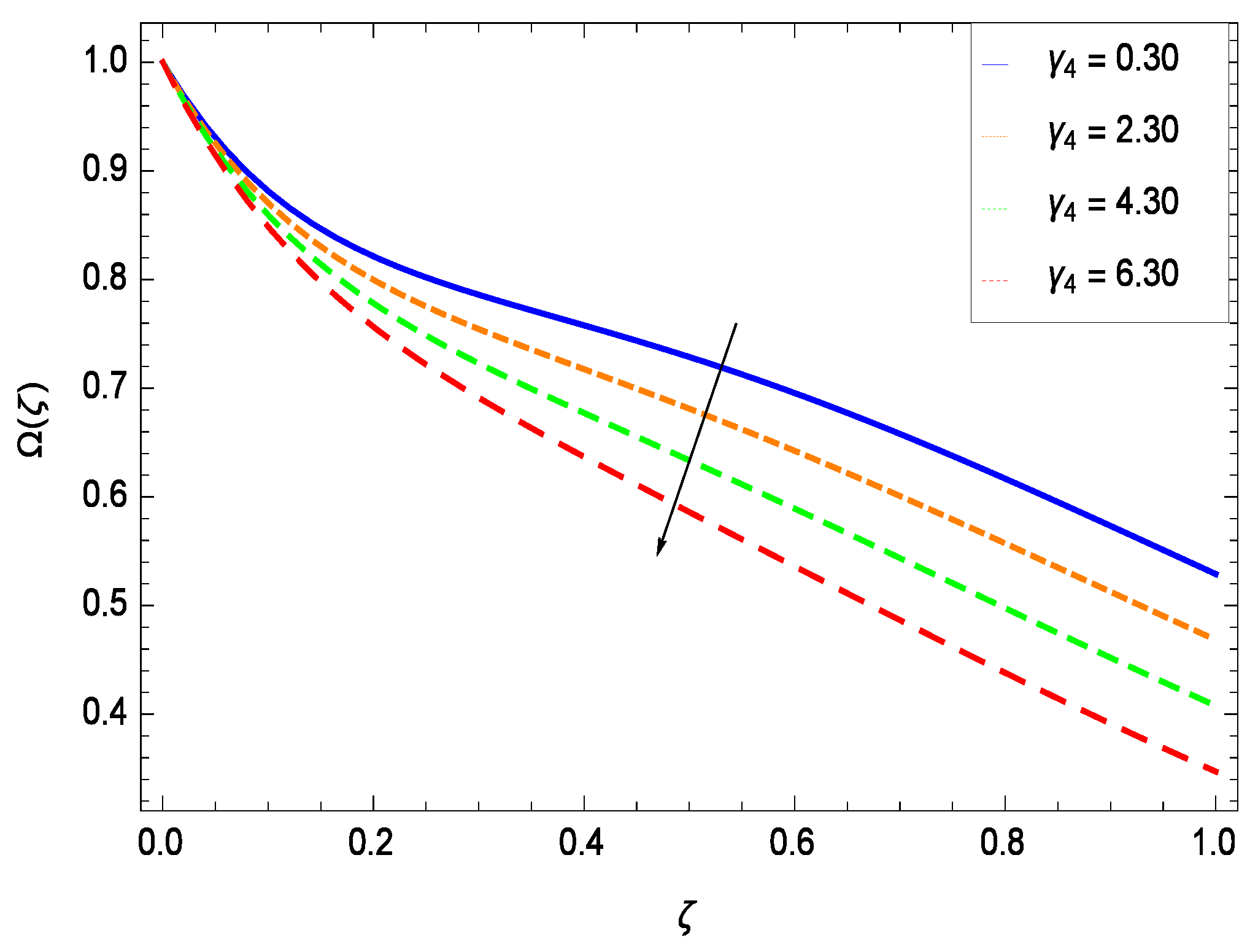
- The temperature () diminishes for the reduced heat transfer parameter , porosity parameter , inertial parameter , magnetic field parameter M and Prandtl number Pr while it elevates for the second grade nanofluid parameter , chemical reaction parameter and thermophoresis parameter Nt.
- (iii)
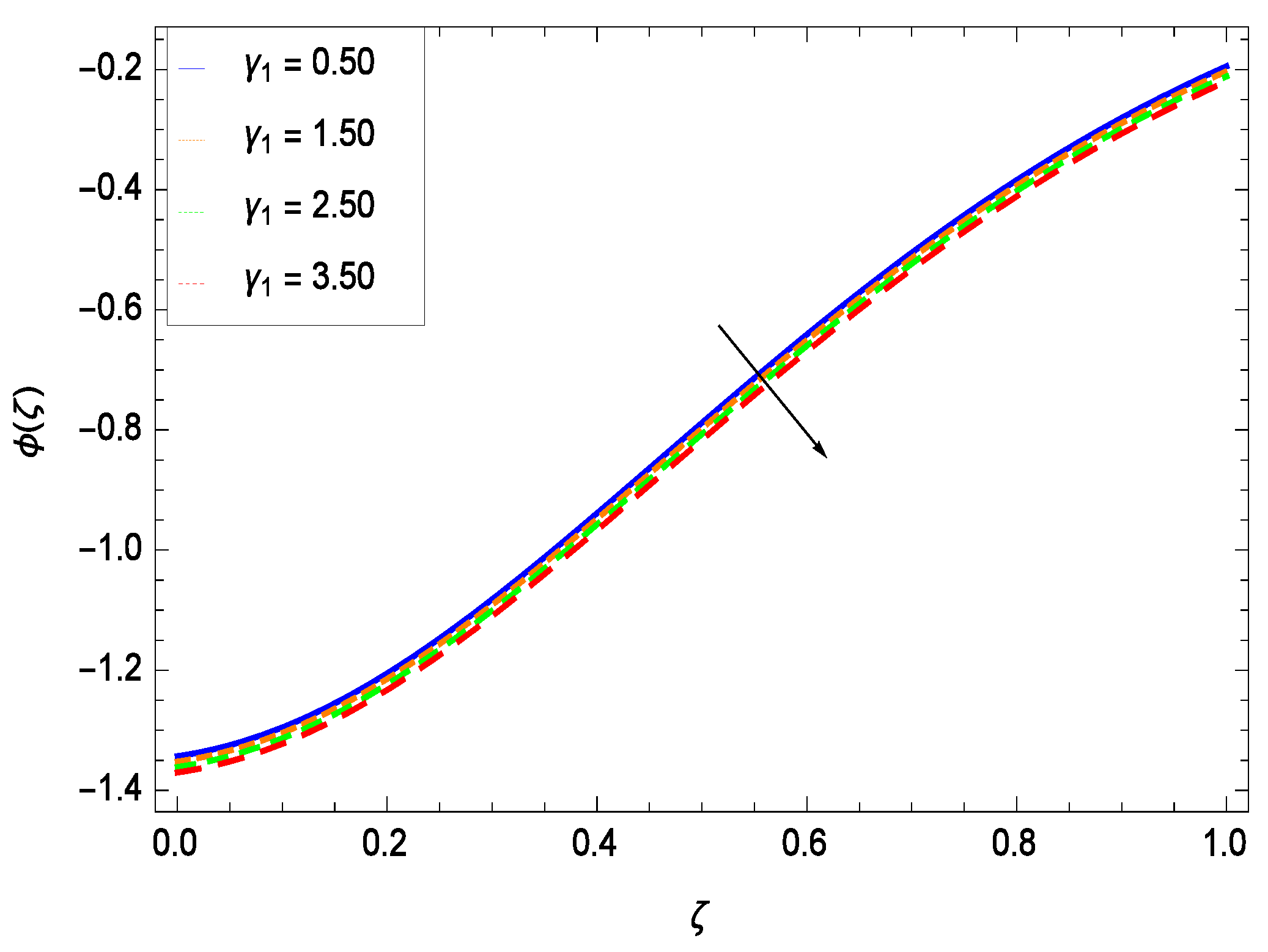
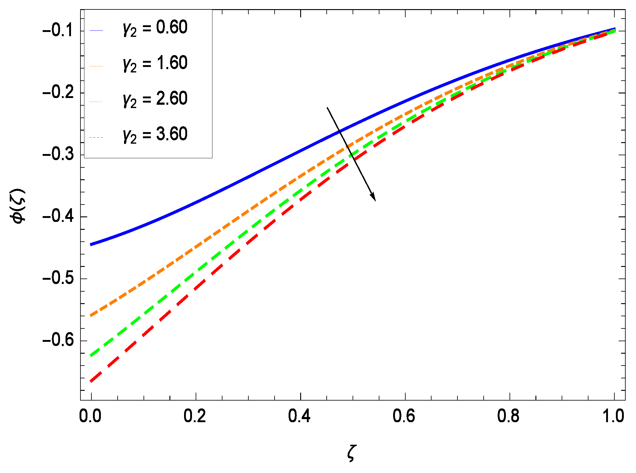
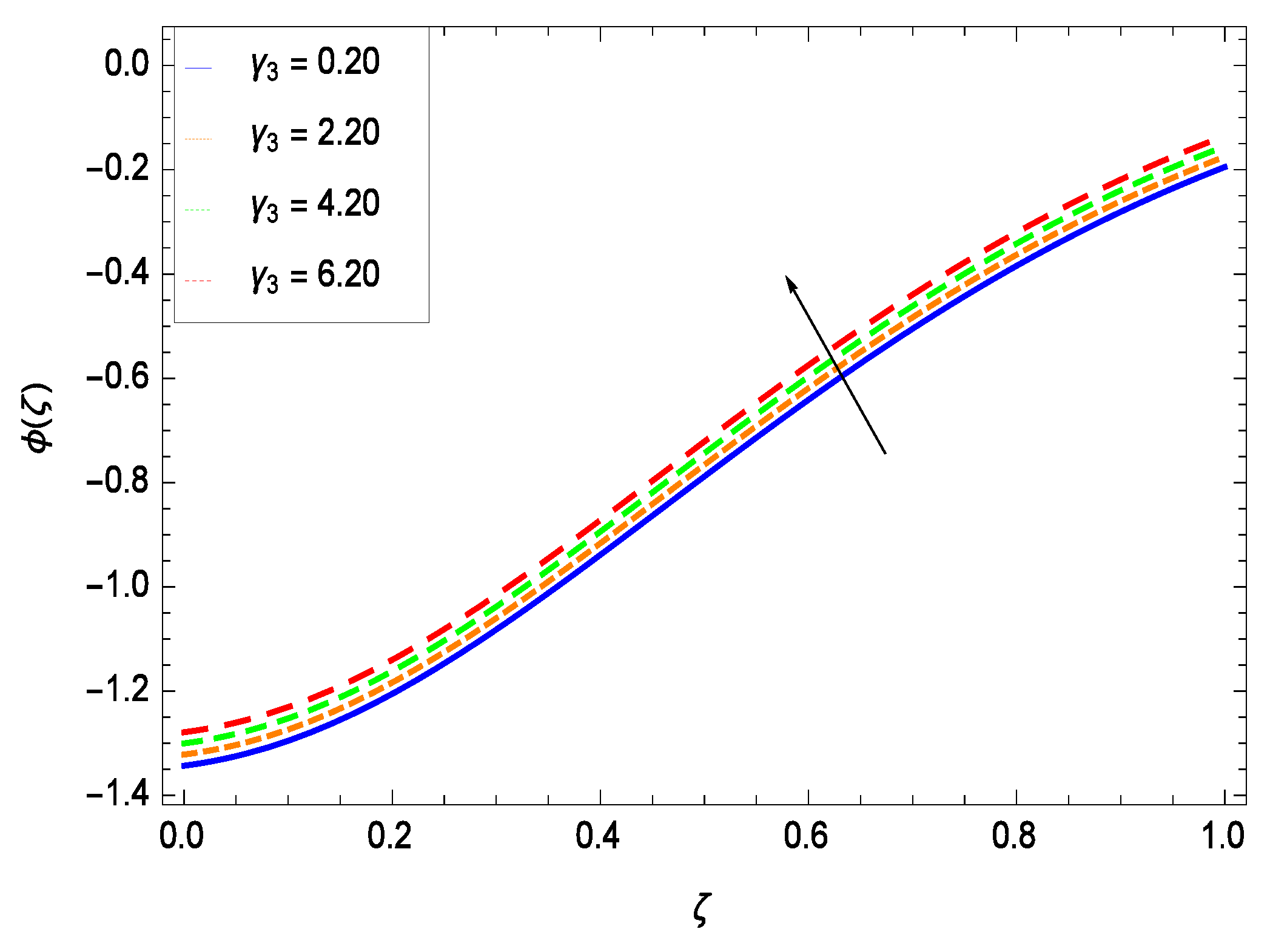
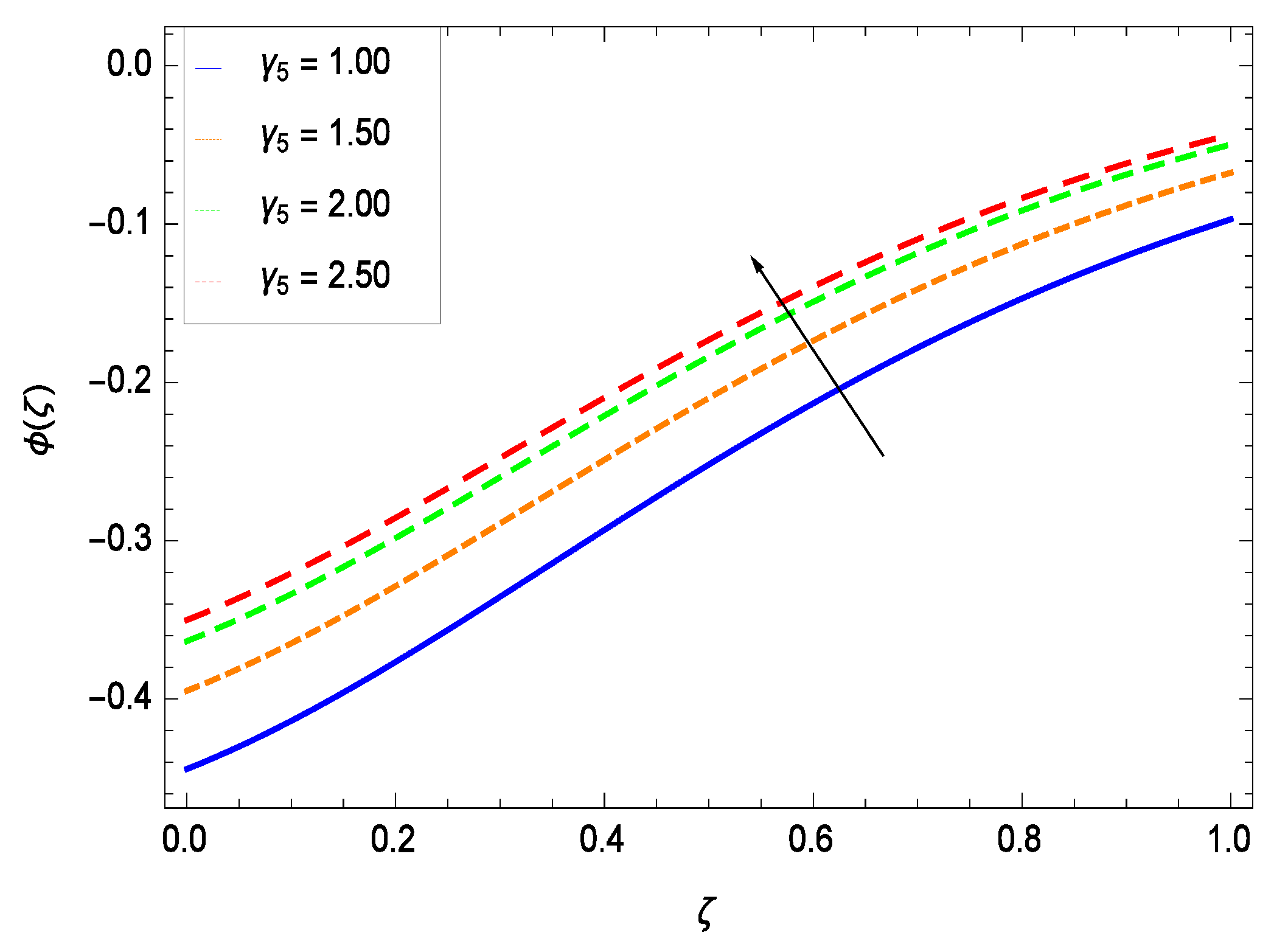
- The nanoparticles concentration () diminishes for second grade nanofluid parameter , reduced heat transfer parameter , thermophoresis parameter Nt and Prandtl number Pr while it elevates for the porosity parameter , inertial parameter , chemical reaction parameter , Brownian motion parameter Nb, Lewis number Le and magnetic field parameter M.
- (iv)
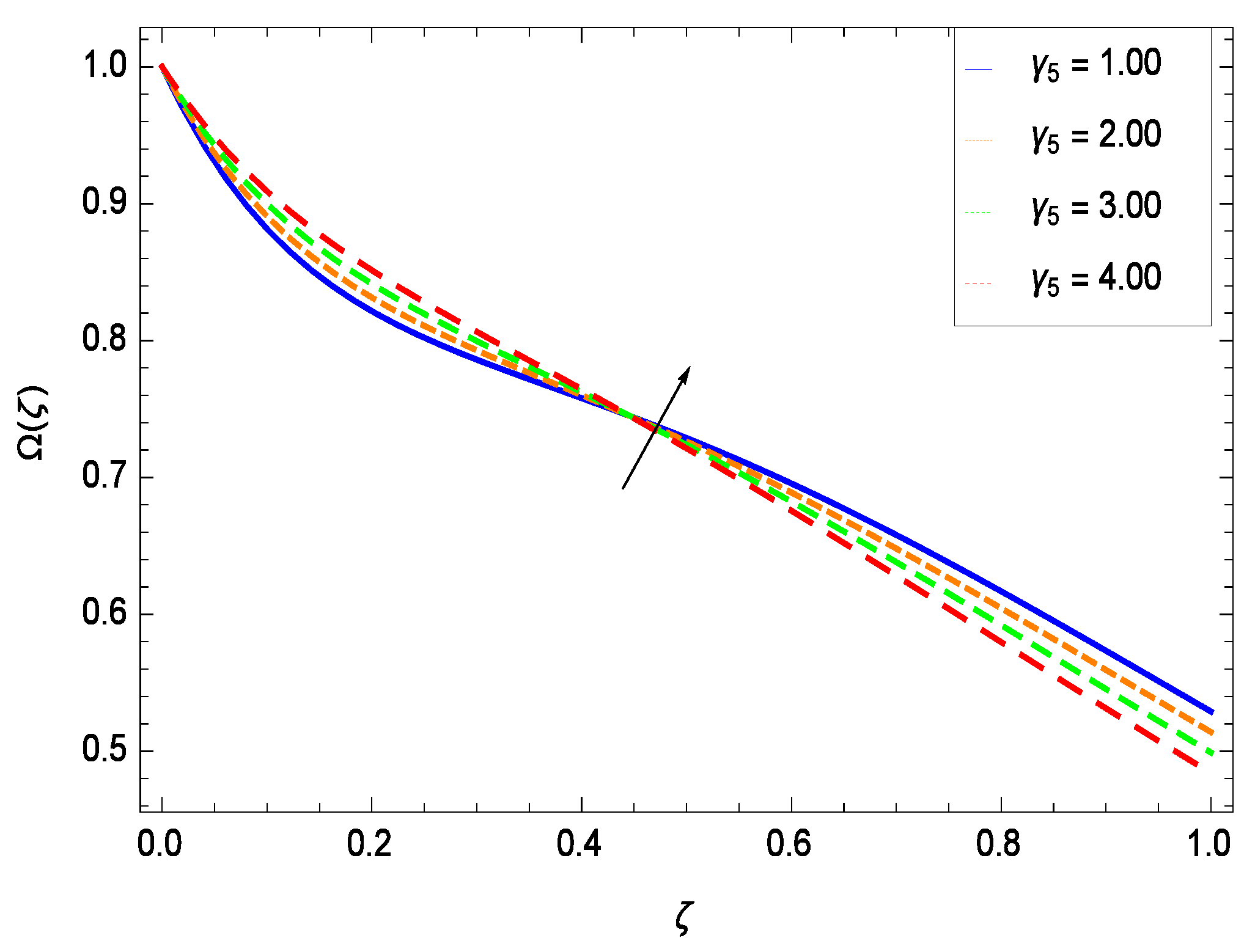
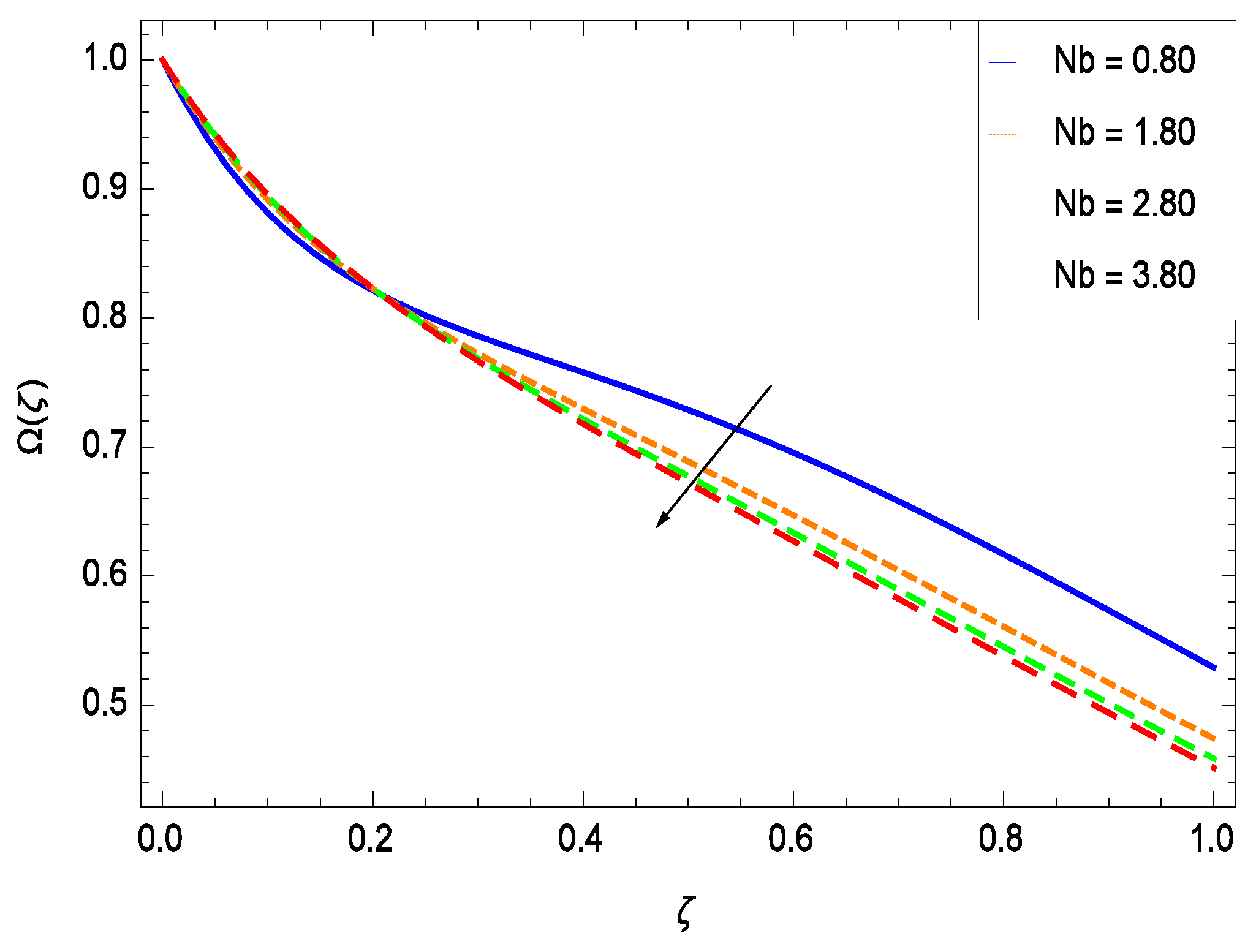
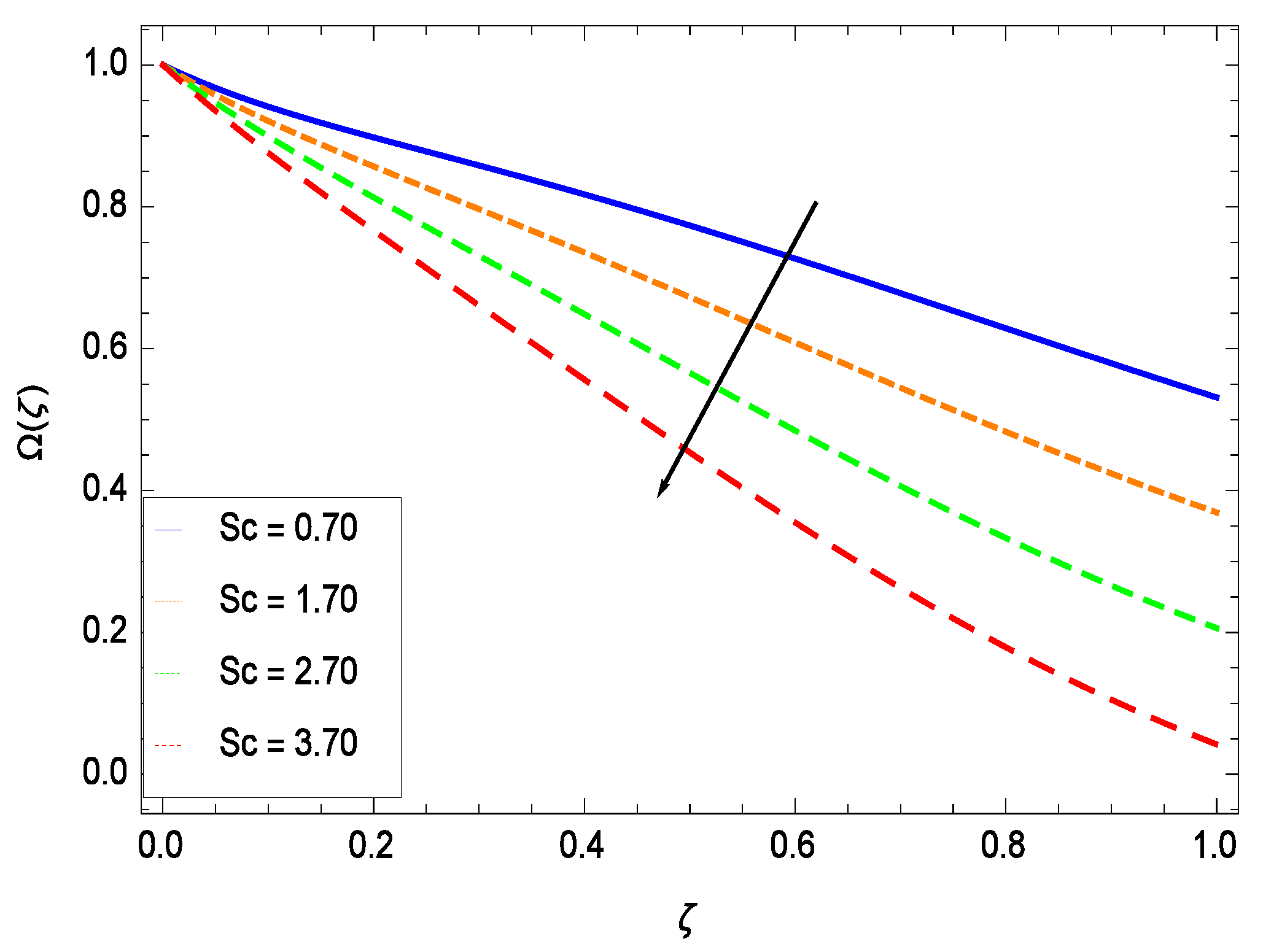
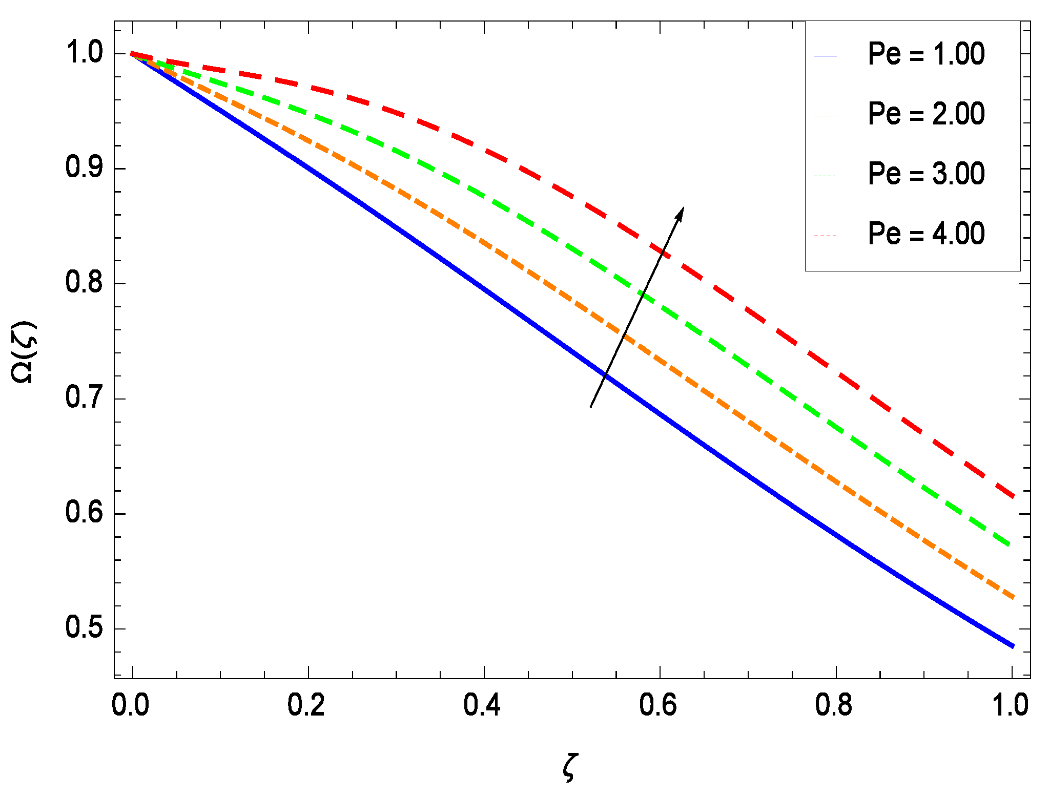
- The microorganism concentration () diminishes for the porosity parameter , inertial parameter , Brownian motion parameter Nb, Schmidt number Sc and magnetic field parameter M while it elevates for the second grade nanofluid parameter , reduced heat parameter , chemical reaction parameter , Lewis number Le, thermophoresis parameter Nt and bioconvection Peclet number Pe.
- (v)
- Entropy generation rate N() diminishes with temperature difference parameter while it elevates for Reynolds number Re, Brinkman number Br, magnetic field parameter M, diffusive constant parameter , nanoparticles concentration difference parameter and microorganism concentration difference parameter .
- (vi)
- Residual errors graphs are self explanatory for the efficiency of HAM solution.
Author Contributions
Funding
Acknowledgments
Conflicts of Interest
Abbreviations
| x | x-axis coordinate (m) |
| y | y-axis coordinate (m) |
| u | Velocity component along x-axis (m s) |
| v | Velocity component along y-axis (m s) |
| Average swimming velocity (m s) | |
| U | Free stream velocity (m s) |
| W | Maximum cell swimming speed (m s) |
| a | Constant |
| b | Chemotaxis constant |
| B | Magnetic flux density (Tesla) |
| Gr | Thermal Grashof number |
| M | Magnetic field parameter |
| Nr | Buoyancy ratio parameter |
| Rb | Bioconvection Rayleigh number |
| Nt | Thermophoresis parameter |
| Nb | Brownian motion parameter |
| Le | Lewis number |
| Sc | Schmidt number |
| Pe | Bioconvection Peclet number |
| Pr | Prandtl number |
| g | Gravitational acceleration (m s) |
| P | Pressure (kg m s) |
| c | Specific heat at constant pressure (J kg K) |
| k | Thermal conductivity (W/m K) |
| T | Temperature (K) |
| T | Convective surface temperature (K) |
| T | Ambient fluid temperature (K) |
| h | Heat transfer coefficient |
| C | Nanoparticles concentration |
| C | Ambient fluid concentration |
| N | Number density of motile microorganisms |
| N | Wall concentration of microorganisms |
| N | Ambient concentration of microorganisms |
| N | Entropy generation number |
| D | Diffusivity |
| D | Brownian diffusion coefficient |
| D | Thermophoretic diffusion coefficient |
| D | Diffusivity of microorganisms |
| f() | Dimensionless velocity |
| L | Characteristic length (m) |
| R | Ideal gas constant |
| Re | Reynolds number |
| Br | Brinkman number |
| Normal stress moduli | |
| Electrical conductivity ((·m)) | |
| Coefficient of viscosity (kg m s) | |
| Density (kg m) | |
| Kinematic viscosity (m s) | |
| Physical stream function (m s) | |
| Coefficient of volumetric volume expansion | |
| Difference operator | |
| Thermal diffusivity of nanofluid (m s) | |
| Ratio of the heat capacitances of nanoparticle and base fluid | |
| A scaled boundary layer coordinate | |
| () | Dimensionless temperature |
| Dimensionless temperature difference | |
| () | Dimensionless concentration |
| Dimensionless concentration difference | |
| () | Dimensionless microorganisms concentration |
| Dimensionless microorganisms concentration difference | |
| Average volume of microorganisms (m) | |
| Dimensionless second grade nanofluid parameter | |
| Reduced heat transfer parameter | |
| Porosity parameter | |
| Inertial parameter | |
| Chemical reaction parameter | |
| Diffusive constant parameter due to nanoparticles concentration | |
| Non-dimensional positive number | |
| Diffusive constant parameter due to microorganisms concentration | |
| av | Average |
| B | Brownian |
| c | Cell |
| p | Solid particles |
| r | Reaction |
| n | Properties related to microorganisms |
| f | Base fluid |
| o | Origin |
| x | Local value |
| w | Properties at the wall |
| ∞ | Fluid properties at ambient condition |
| Superscripts | |
| s | Swimming |
| ′ | Differentiation w. r. t. |
References
- Khan, N.S.; Zuhra, Z.; Shah, Z.; Bonyah, E.; Khan, W.; Islam, S. Hall current and thermophoresis effects on magnetohydrodynamic mixed convective heat and mass transfer thin film flow. J. Phys. Commun. 2018. [Google Scholar] [CrossRef]
- Ishaq, M.; Ali, M.; Shah, Z.; Islam, S.; Muhammad, S. Entropy generation on nanofluid thin film flow of Eyring-Powell fluid with thermal radiation and MHD effect on an unsteady porous stretching sheet. Entropy 2018, 6. [Google Scholar] [CrossRef]
- Hayat, T.; Khan, M.I.; Qayyum, S.; Khan, M.I.; Alsaedi, A. Entropy generation for flow of Sisko fluid to rotating disk. J. Mol. Liquids 2018, 264, 375–385. [Google Scholar] [CrossRef]
- Khan, N.S.; Gul, T.; Khan, M.A.; Bonyah, E.; Islam, S. Mixed convection in gravity-driven thin film non-Newtonian nanofluids flow with gyrotactic microorganisms. Results Phys. 2017, 7, 4033–4049. [Google Scholar] [CrossRef]
- Zuhra, S.; Khan, N.S.; Islam, S. Magnetohydrodynamic second grade nanofluid flow containing nanoparticles and gyrotactic microorganisms. Comput. Appl. Math. 2018, 37, 6332–6358. [Google Scholar] [CrossRef]
- Khan, N.S. Bioconvection in second grade nanofluid flow containing nanoparticles and gyrotactic microorganisms. Braz. J. Phys. 2018, 43, 227–241. [Google Scholar] [CrossRef]
- Palwasha, Z.; Islam, S.; Khan, N.S.; Ayaz, H. Non-Newtonian nanoliquids thin film flow through a porous medium with magnetotactic microorganisms. Appl. Nanosci. 2018, 8, 1523–1544. [Google Scholar] [CrossRef]
- Raees, A.; Xu, H.; Liao, S.J. Unsteady mixed nano-bioconvection flow in a horizontal channel with its upper plate expanding or contracting. Int. J. Heat Mass Transf. 2015, 86, 174–182. [Google Scholar] [CrossRef]
- Zuhra, S.; Khan, N.S.; Shah, Z.; Islam, S.; Bonyah, E. Simulation of bioconvection in the suspension of second grade nanofluid containing nanoparticles and gyrotactic microorganisms. AIP Adv. 2018, 8, 105210. [Google Scholar] [CrossRef]
- Pedley, T.J. Instability of uniform microorganism suspensions revisited. J. Fluid Mech. 2010, 647, 335–359. [Google Scholar] [CrossRef]
- Xu, H.; Pop, I. Mixed convection flow of a nanofluid over a stretching surface with uniform free stream in the presence of both nanoparticles and gyrotactic microorganisms. Int. J. Heat Mass Transf. 2014, 75, 610–623. [Google Scholar] [CrossRef]
- Aziz, A.; Khan, W.A.; Pop, I. Free convection boundary layer flow past a horizontal flat plate embedded in porous medium filled by nanofluid containing gyrotactic microorganisms. Int. J. Therm. Sci. 2012, 56, 48–57. [Google Scholar] [CrossRef]
- Bhatti, M.M.; Mishra, S.R.; Abbas, T.; Rashidi, M.M. A mathematical model of MHD nanofluid flow having gyrotactic microorganisms with thermal radiation and chemical reaction effects. Neural Comput. Appl. 2016. [Google Scholar] [CrossRef]
- Raees, A.; Xu, H.; Sun, Q.; Pop, I. Mixed convection in gravity-driven nanoliquid film containing both nanoparticles and gyrotactic microorganisms. Appl. Math. Mech. 2015, 36, 163–178. [Google Scholar] [CrossRef]
- Ramzan, M.; Chung, J.D. Naeem Ullah, Radiative magnetohydrodynamic nanofluid flow due to gyrotactic microorganisms with chemical reaction and non-linear thermal radiation. Int. J. Mech. Sci. 2017. [Google Scholar] [CrossRef]
- Anjalidevi, S.P.; Kandasamy, R. Effects of chemical reaction, heat and mass transfer on laminar flow along a semi infinite horizontal plate. Heat Mass Transf. 1999, 35, 465–467. [Google Scholar] [CrossRef]
- Khan, N.S.; Gul, T.; Islam, S.; Khan, W. Thermophoresis and thermal radiation with heat and mass transfer in a magnetohydrodynamic thin film second-grade fluid of variable properties past a stretching sheet. Eur. Phys. J. Plus 2017, 132. [Google Scholar] [CrossRef]
- Palwasha, Z.; Khan, N.S.; Shah, Z.; Islam, S.; Bonyah, E. Study of two-dimensional boundary layer thin film fluid flow with variable thermophysical properties in three dimensions space. AIP Adv. 2018, 8, 105318. [Google Scholar] [CrossRef]
- Khan, N.S.; Zuhra, S.; Shah, Z.; Bonyah, E.; Khan, W.; Islam, S. Slip flow of Eyring-Powell nanoliquid film containing graphene nanoparticles. AIP Adv. 2018, 8, 115302. [Google Scholar] [CrossRef]
- Zuhra, S.; Khan, N.S.; Khan, M.A.; Islam, S.; Khan, W.; Bonyah, E. Flow and heat transfer in water based liquid film fluids dispensed with graphene nanoparticles. Results Phys. 2018, 8, 1143–1157. [Google Scholar] [CrossRef]
- Khan, N.S.; Gul, T.; Islam, S.; Khan, I.; Alqahtani, A.M.; Alshomrani, A.S. Magnetohydrodynamic nanoliquid thin film sprayed on a stretching cylinder with heat transfer. J. Appl. Sci. 2017, 7, 271. [Google Scholar] [CrossRef]
- Khan, N.S.; Gul, T.; Islam, S.; Khan, A.; Shah, Z. Brownian motion and thermophoresis effects on MHD mixed convective thin film second-grade nanofluid flow with Hall effect and heat transfer past a stretching sheet. J. Nanofluids 2017, 6, 812–829. [Google Scholar] [CrossRef]
- Khan, N.S.; Gul, T.; Islam, S.; Khan, W.; Khan, I.; Ali, L. Thin film flow of a second-grade fluid in a porous medium past a stretching sheet with heat transfer. Alex. Eng. J. 2017. [Google Scholar] [CrossRef]
- Wu, M.; Kuznetsov, A.V.; Jasper, W.J. Modeling of particle trajectories in an electro-statically charged channel. Phys. Fluids 2011, 22, 043301. [Google Scholar] [CrossRef]
- Kuznetsov, A.V. Emerging Topics in Heat and Mass Transfer in Porous Media, From Bioengineering and Microelectronics to Nanotechnology; Springer: Dordrecht, The Netherlands, 2012. [Google Scholar]
- Tham, L.; Nazar, R.; Pop, I. Steady mixed convection boundary layer flow on a horizontal circular cylinder with a constant surface temperature embedded in a porous medium saturated by a nanofluid containing both nanoparticles and gyrotactic microorganisms. J. Heat Transf. 2013, 135, 102601-1. [Google Scholar] [CrossRef]
- Liao, S.J. Homotopy Analysis Method in Nonlinear Differential Equations; Higher Education Press: Beijing, China; Springer: Berlin/Heidelberg, Germany, 2012. [Google Scholar]


| Author Names | Author Works | Some Outcomes |
|---|---|---|
| Khan et al. [1] | Entropy generation | Entropy generation increases with Reynolds number |
| Ishaq et al. [2] | Entropy generation | Entropy generation decreases with Eyring-Powell parameter |
| Hayat et al. [3] | Entropy generation | Entropy generation increases with Reynolds number |
| Khan et al. [4] | Bioconvection | Bioconvection decreases with reduced heat transfer parameter |
| Zuhra et al. [5] | Bioconvection | Gyrotactic microorganisms depreciates with magnetic field parameter |
| Khan [6] | Bioconvection | Stratification increases with second-grade fluid parameter |
| Palwasha et al. [7] | Bioconvection | Stratification increases with gravitational forces |
| Raees et al. [8] | Bioconvection | Bioconvection depends on upper plate |
| Zuhra et al. [9] | Bioconvection | Microorganisms decrease with increasing Brownian motion parameter |
| Pedley [10] | Instability | Instability of the system is due to microorganisms |
| Xu et al. [11] | Mixed convection | Nanoparticles favor the mixed convection |
| Aziz et al. [12] | Free convection | Instability of the system increases due to microorganisms |
| Bhatti et al. [13] | Chemical reaction | Mass transfer increases with chemical reaction |
| Raees et al. [14] | Bioconvection‘ | Passively controlled nanofluid model provides better results |
| Ramzan et al. [15] | Chemical reaction | Mass transfer increases with chemical reaction |
| Anjalidevi [16] | Chemical reaction | Mass transfer increases with chemical reaction |
| Parameter Names | Symbols/Notations | Defined Values |
|---|---|---|
| Dimensionless second-grade nanofluid parameter | ||
| Thermal Grashof number | Gr | |
| Buoyancy ratio parameter | Nr | |
| Bioconvection Rayleigh number | Rb | |
| Prandtl number | Pr | |
| Thermophoresis parameter | Nt | |
| Brownian motion parameter | Nb | |
| Lewis number | Le | |
| Schmidt number | Sc | |
| Bioconvection Peclet number | Pe | |
| Reduced heat transfer parameter | ||
| Porosity parameter | ||
| Inertial parameter | ||
| Chemical reaction parameter | ||
| Magnetic field parameter | M |
© 2019 by the authors. Licensee MDPI, Basel, Switzerland. This article is an open access article distributed under the terms and conditions of the Creative Commons Attribution (CC BY) license (http://creativecommons.org/licenses/by/4.0/).
Share and Cite
Khan, N.S.; Shah, Z.; Islam, S.; Khan, I.; Alkanhal, T.A.; Tlili, I. Entropy Generation in MHD Mixed Convection Non-Newtonian Second-Grade Nanoliquid Thin Film Flow through a Porous Medium with Chemical Reaction and Stratification. Entropy 2019, 21, 139. https://doi.org/10.3390/e21020139
Khan NS, Shah Z, Islam S, Khan I, Alkanhal TA, Tlili I. Entropy Generation in MHD Mixed Convection Non-Newtonian Second-Grade Nanoliquid Thin Film Flow through a Porous Medium with Chemical Reaction and Stratification. Entropy. 2019; 21(2):139. https://doi.org/10.3390/e21020139
Chicago/Turabian StyleKhan, Noor Saeed, Zahir Shah, Saeed Islam, Ilyas Khan, Tawfeeq Abdullah Alkanhal, and Iskander Tlili. 2019. "Entropy Generation in MHD Mixed Convection Non-Newtonian Second-Grade Nanoliquid Thin Film Flow through a Porous Medium with Chemical Reaction and Stratification" Entropy 21, no. 2: 139. https://doi.org/10.3390/e21020139