Simulation and Characterization of Wind Impacts on sUAS Flight Performance for Crash Scene Reconstruction

Abstract

Small unmanned aircraft systems (sUASs) have emerged as promising platforms for the purpose of crash scene reconstruction through structure-from-motion (SfM) photogrammetry. However, auto crashes tend to occur under adverse weather conditions that usually pose increased risks of sUAS operation in the sky. Wind is a typical environmental factor that can cause adverse weather, and sUAS responses to various wind conditions have been understudied in the past. To bridge this gap, commercial and open source sUAS flight simulation software is employed in this study to analyze the impacts of wind speed, direction, and turbulence on the ability of sUAS to track the pre-planned path and endurance of the flight mission. This simulation uses typical flight capabilities of quadcopter sUAS platforms that have been increasingly used for traffic incident management. Incremental increases in wind speed, direction, and turbulence are conducted. Average 3D error, standard deviation, battery use, and flight time are used as statistical metrics to characterize the wind impacts on flight stability and endurance. Both statistical and visual analytics are performed. Simulation results suggest operating the simulated quadcopter type when wind speed is less than 11 m/s under light to moderate turbulence levels for optimal flight performance in crash scene reconstruction missions, measured in terms of positional accuracy, required flight time, and battery use. Major lessons learned for real-world quadcopter sUAS flight design in windy conditions for crash scene mapping are also documented.

1. Introduction

A motor vehicle crash can cause considerable economic loss, serious bodily injuries and loss of human life. Crash scene investigation and reconstruction are considered crucial being part of the major concerns in traffic incident management (TIM) [1]. Traditional coordinate and triangulation methods have long been adopted by investigators at a crash scene. They use mechanical measurement tools such as tape measures and roller wheels to acquire baseline measurements and delineate crash scene diagrams [2]. While relatively low cost, these methods have limited efficiency to document measurements and pose safety risks to investigators due to possible exposure to traffic. In order to automate accurate documentation of distance and angle measurements, total stations have started to play a key role at crash scenes since the early 1990s [3]. The ability to collect digital data off the roadway eases investigators’ exposure risk to traffic and reduces entire surveying time. Close-range photogrammetry, which emerged around the same time in accident investigation, is able to recover accurate two-dimensional (2D) and three-dimensional (3D) measurements and diagrams by taking overlapping photographs from different viewpoints around crash scenes [4]. Over the past two decades, the potential of terrestrial laser scanning (TLS) has been validated in various crash scene scenarios [5,6,7]. Enormous scene details can be scanned and captured in a relatively short period of time. However, the costs of TLS equipment are usually high, and multiple scan locations may be needed to minimize scan occlusions in scenes where terrain and crash are complex.

With rapid advances in microelectronics, radio communication, miniaturized imaging lenses and positioning modules, small unmanned aircraft systems (sUASs) have pioneered a series of TIM applications, such as traffic monitoring, flow analysis, crash detection and response, and situational awareness [8,9,10]. Advantages of using sUAS platforms for TIM include: (1) allowing for customization of onboard sensing systems and observing parameters, (2) offering adequate flexibility in data collection above the scene to be investigated, (3) reducing the exposure of investigators to the dangers of traffic in the roadway, and (4) providing detailed 2D and/or 3D measurement documentation and imagery for post-crash scene investigation conducted in the office. Nowadays, the potential of multirotor sUASs being low-cost and robust crash scene recovery platforms has been manifested via structure-from-motion (SfM) photogrammetry. SfM converts overlapped image sequences taken by a consumer-grade digital camera into 2D orthorectified image products and reconstructed 3D scenes (dense 3D point cloud data and textured 3D meshes). SfM photogrammetry with an octocopter platform was reported to save up to 90% of data collection time compared with traditional coordinate method [11]. Measurements obtained from the point cloud were in accordance with sketches drawn by the investigators, and centimeter-level differences were found in the entire scene. Above the accident scene, orthophotos can be generated using a sequence of individual photos converted from the 4 K-resolution video taken by the quadcopter camera [12]. The results demonstrated a horizontal accuracy of 5–8 cm in scene documentation compared with a real time kinematic (RTK) global navigation satellite system (GNSS) survey.

While growing attention has been paid to SfM photogrammetric surveys with sUAS platforms in crash scene investigation and recovery, it is important to realize that nearly 21% of the crashes are weather-related every year in the United States [13] and performing flight missions under hazardous weather conditions remains a difficult task due to safety and data quality concerns. For example, wind is a frequent natural phenomenon, but high winds tend to increase the risks of freight truck crashes on the roadway [14,15]. In such a scenario, before an sUAS is dispatched to conduct the crash scene reconstruction mission, it is essential to ensure that the wind speed does not exceed the aircraft’s operation limit specified by the vendor. Some sUASs are less susceptible to the wind disturbance, but their battery life and flight time is reduced as wind speeds increase [16,17]. High wind speed can also negatively affect the SfM photogrammetry and derived mapping products due to disturbed waypoint targeting and image orientation. Wind direction and turbulence are also important variables to consider as they affect the flight path geometry, energy consumption and overall flight safety [18,19,20,21].

Some studies have documented preliminary findings on the variations of sUAS flight stability due to wind forces. Wang conducted an in-house simulation to assess the wind impacts on sUAS flight stability at low altitudes [22]. The differences in flight speed and attitude were summarized when various types of wind were examined. Siqueira mathematically created a wind model and evaluated its effects on sUAS trajectory tracking by looking into 2D/3D error and control activities [23]. The results suggested rapid trajectory tracking degradation as a response to the increased magnitude of wind dynamics.

Initial research efforts have been made in recent years to use open-source mission planning tools such as Mission Planner to conduct sUAS simulation runs in windy conditions [24]. However, comprehensively characterizing sUAS responses to various wind conditions has been understudied but is considered crucial before planning flight operations for crash scene reconstruction. While there are multiple types of suboptimal weather conditions that raise safety and data quality concerns for flying sUASs, the main aim of this study is to set wind as an exclusive factor to parameterize its impacts on flight performance of a representative quadcopter sUAS platform type via realistic flight simulations using a standard gridded flight design for SfM image acquisition. Simulation results are applied to document and generalize lessons learned for platform-independent quadcopter sUAS flight design under windy conditions for crash scene mapping. A series of quadcopter simulations with incremental increases in wind speed, direction, and turbulence are performed to model suboptimal weather conditions. Positional error, battery use, and flight time are used as statistical metrics to characterize the wind impacts on flight performance.

2. Materials and Methods

2.1. Test Environment Setup

As the most popular open-source autopilot software suite adopted by a variety of autonomous vehicles, ArduPilot was employed as the underlying simulation framework in this study [25,26,27]. ArduPilot enables modeling a wide range of unmanned vehicle characteristics with regard to mission planning, remote control, communication and navigation. To realistically characterize wind impacts on sUAS behavior in a simulated environment, the software-in-the-loop (SITL) simulator was run on a host computer without risking an actual aircraft platform. ArduPilot on SITL can compile source code based on a sophisticated sUAS flight dynamics model and perform code execution in software environment for development and testing purposes. In such a simulation framework, ArduPilot supports the MAVLink protocol for real-time telemetry between the simulated sUAS and the ground control station (GCS) such as Mission Planner. Mission Planner as an open-source GCS includes major flight planning functions similar to that in commercial software packages such as Pix4Dcapture and Map Pilot Pro. In this work, Mission Planner along with ArduPilot on SITL was used for flight simulation, which enabled: (1) editing various parameters regarding changes in environment type, sensor failure and vehicle platform, (2) simulating an sUAS as a virtual flight control unit (FCU) to conduct pre-defined simulation runs on a computer without any special hardware, and (3) storing and downloading the log files of a mission for post-flight analysis.

In the United States, quadcopter sUAS platforms have been widely chosen and increasingly used for TIM and crash scene reconstruction by law enforcement agencies [9,28,29,30,31,32]. Compared with other frame types, such as hexacopters and octocopters, quadcopters can be designed and developed relatively cheap and small in size for carrying positioning and non-metric camera payloads to perform SfM photogrammetric tasks. This study, therefore, selected a quadcopter frame type to run realistic simulations in ArduPilot SITL to characterize wind impacts on flight performance for crash scene reconstruction. This quadcopter frame type has been employed by some commercial platforms including 3DR Solo and Parrot Bebop 2 [33,34]. It is possible to edit a list of behavior controlling parameters through the MAVLink protocol. A complete set of such parameters is available in [35].

A rectangular area at the Texas A&M Flight Test Station Airport in Bryan, Texas, USA, was identified to define the boundary of the simulated crash scene. The rectangular area was 105 × 70 m and centered over an airfield intersection at 30°38′16.50″ N, 96°28′54.70″ W. In this work, a DJI Mavic 2 Pro camera model was selected in Mission Planner due to its current popularity in use by law enforcement and transportation agencies for crash scene mapping [28,29,30]. In this study, two flight paths were planned in simulation as follows:

I.

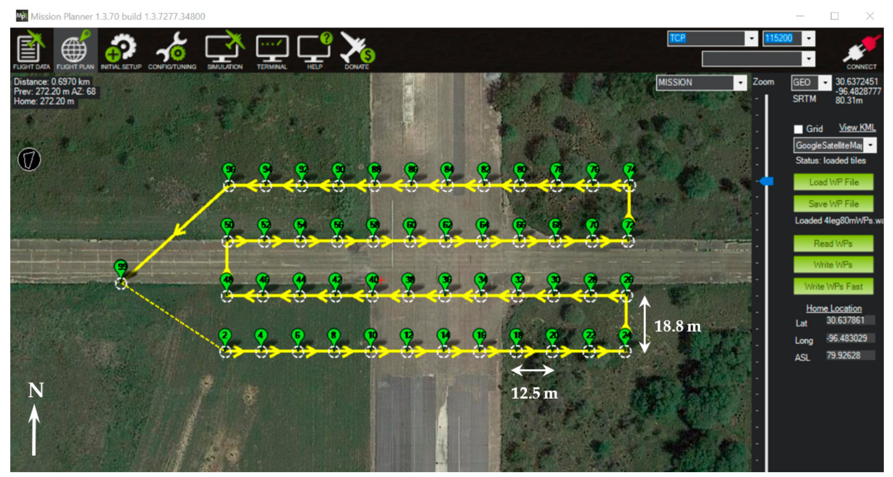
A single flight height of 80 m above ground level (AGL) was determined, targeting a ground sample distance (GSD) of 2.0 cm/px to enable capturing crash scene details. The flight mission intended to achieve 80% frontal and 80% side overlap to facilitate creation of adequate SfM photogrammetric mapping products [36,37], resulting in 48 photo locations taken along four flight lines in the East-West course (i.e., flight direction) with 12 photo locations along each (Figure 1). The flight plan included the sUAS stopping at each waypoint location to capture an image before moving to the next waypoint. The spacing between adjacent waypoints was 12.5 m and the spacing between flight lines was 18.8 m.

II.

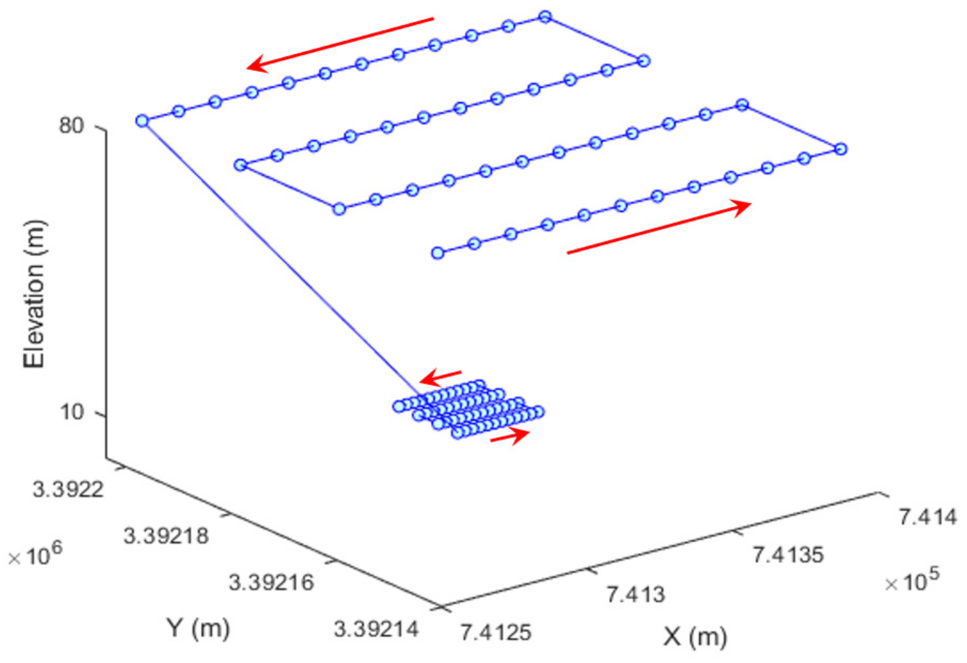
Simulations ran at dual altitudes of 80 m and 10 m AGL. In this flight path, the simulated quadcopter first completed an entire set of actions at 80 m AGL as defined in flight path I, then it descended and continued the mission at 10 m AGL (Figure 2). At this lower altitude, the flight courses were kept the same, and 80% frontal and 80% side overlap settings remained. At 10 m AGL, an additional 48 photos were acquired along four flight lines that were scaled down. At 10 m AGL, the spacing between waypoints was 2.5 m and the spacing between flight lines was 3.7 m.

It is worth noting that in an SfM photogrammetric survey mission, the flight height relates closely to the length of a mission and waypoint locations given specific overlap and camera model settings. However, the flight height is independent to simulated wind effects to be defined in Section 2.2. In other words, the choice of flight height is generic in this study and another flight altitude will not vary wind impacts compared with that of 80 m or 10 m AGL.

Mission Planner placed the simulated aircraft at the home position near the mission scene. The SITL ran a simulated FCU within the virtual aircraft and the planned actions were then uploaded into the aircraft via the simulated GCS link the same way it would be done in a real flight with an actual aircraft. The interface then allowed setting environmental factors for each simulation run such as wind speed, direction, and turbulence. In this article, these three wind parameters were the primary variables to study the sUAS responses.

2.2. Creation of Simulation Runs

2.2.1. Wind Speed

For single-altitude flight path at 80 m AGL (Figure 1), five values were evaluated with regard to wind speed, which were 0 m/s, 3.5 m/s, 7.0 m/s, 10.5 m/s, and 14 m/s. The value of 14 m/s was chosen as the upper bound because after this level, the respective quadcopter frame selected in Mission Planner’s SITL would not be able to maintain its position and started to drift off of the simulated crash scene. For dual-altitude flight path (Figure 2), wind speeds of 10.5 m/s and 3.5 m/s were employed at 80 m and 10 m AGL, respectively.

2.2.2. Wind Direction

Wind direction is defined as the direction from which the wind is coming with respect to North in a clockwise fashion. For example, 0° represents North wind blowing from North to South and 90° represents East wind blowing from East to West. As described in Figure 1 and Figure 2, the flight lines were oriented in the East-West direction, therefore, without loss of generality, simulating wind directions in the first quadrant (i.e., from 0° to 90°) was sufficient to depict distinct aircraft-wind angular relationships. This angular relationship is defined as α angle, which refers to the included angle from wind direction to flight course moving in a clockwise motion. In this work, the wind directions of 0°, 22.5°, 45°, 67.5°, and 90° were chosen for single-altitude flight path at 80 m AGL (Figure 1), the wind directions of 0°, 45°, and 90° were chosen for dual-altitude flight path at 80 m and 10 m AGL (Figure 2). The α angle and its relation to the wind direction and flight course are summarized in

Table 1. α angle and its relation to the wind direction and flight course.

α Angle	Wind Direction (°)	Flight Course
0° (Headwind)	90°	E
180° (Tailwind)	90°	W
90° (Crosswind)	0°	E
270° (Crosswind)	0°	W
67.5°	22.5°	E
247.5°	22.5°	W
45°	45°	E
225°	45°	W
22.5°	67.5°	E
202.5°	67.5°	W

. In the case of wind direction of 90°, wind blew in or against the direction of aircraft travel, yielding pure tailwind or headwind, respectively. A 0° wind direction generated pure crosswind scenarios where the wind blew perpendicular to the flight path. All the other wind directions were able to decompose the force into both crosswind and headwind/tailwind components, and the corresponding α angles are illustrated in Figure 3.

2.2.3. Turbulence

Turbulence takes place by adding 3D random vectors and magnitudes to the existing wind conditions. According to the National Weather Service, turbulence for operating aircraft is classified as [38]:

• Light (less than 7.2 m/s, and less than 5.7 m/s vertically),
• Moderate (7.2–12.3 m/s, and 5.7–11.3 m/s vertically),
• Severe (greater than 12.3 m/s, and 11.3–14.9 m/s vertically), and
• Extreme (greater than 12.3 m/s, and greater than 14.9 m/s vertically).

Within ArduPilot on SITL, turbulence is modeled as a combination of high pass and low pass filters in both horizontal and vertical directions satisfying the following conditions [39]

$$t_h^n=0.98 t_h^{n-1}+10·\left(1-0.98\right)t_i{r}_g$$

(1)

$$t_v^n=0.98 t_v^{n-1}+10·\left(1-0.98\right)t_i{r}_g$$

(2)

where $t_h$ and $t_v$ represent horizontal and vertical turbulences in the unit of m/s, respectively, $n$ and $n-1$ denote current and previous time instances, $r_g$ is a random number following a $\mathcal{N}\left(0, 1\right)$ Gaussian distribution, and $t_i$ is a turbulence index value set to 0, 5, 10, or 20 in this work. As the turbulence index increased, the turbulence magnitude increased. More specifically, a turbulence index of five (i.e., $t_i=5$ in Equations (1) and (2)) involved randomized horizontal and vertical air speed fluctuations as great as 5 m/s. Likewise, turbulence indices of 10 and 20 (i.e., $t_i=10$and 20 in Equations (1) and (2)) involved randomized horizontal and vertical air fluctuations as great as 10 m/s and 20 m/s, respectively. For single-altitude flight path at 80 m AGL as shown in Figure 1, light (i.e., turbulence indices of 0 and 5), moderate (i.e., turbulence index of 10), and extreme (i.e., turbulence index of 20) turbulence conditions were simulated. It was not necessary to simulate severe turbulence because the only difference between severe and extreme turbulences was the vertical turbulence component. For dual-altitude flight path at 80 m and 10 m AGL as shown in Figure 2, light (i.e., turbulence index of 0) and moderate (i.e., turbulence index of 10) turbulence conditions were simulated.

It is worth noting that turbulence does not equate to wind gust. Gust denotes a local maximum above a certain threshold above the mean wind speed within a certain amount of time such as one or two minutes [40].

2.2.4. Overview of Simulation Runs

The incrementally increased wind speed, direction, and turbulence values resulted in 58 simulation runs at single altitude of 80 m AGL to evaluate flight stability and endurance (

Table 2. A total of 58 simulation runs with incrementally increased wind speed, direction and turbulence values at single altitude of 80 m AGL.

Wind Direction (°)	Wind Speed (m/s)	Turbulence Index	Flight Height AGL (m)
N/A	0.0	0	80
0	3.5	0	80
0	7.0	0	80
0	10.5	0	80
0	14.0	0	80
22.5	3.5	0	80
22.5	7.0	0	80
22.5	10.5	0	80
22.5	14.0	0	80
45	3.5	0	80
45	7.0	0	80
45	10.5	0	80
45	14.0	0	80
67.5	3.5	0	80
67.5	7.0	0	80
67.5	10.5	0	80
67.5	14.0	0	80
90	3.5	0	80
90	7.0	0	80
90	10.5	0	80
90	14.0	0	80
0	10.5	5	80
22.5	10.5	5	80
45	10.5	5	80
67.5	10.5	5	80
90	10.5	5	80
0	0.0	10	80
0	3.5	10	80
0	7.0	10	80
0	10.5	10	80
22.5	3.5	10	80
22.5	7.0	10	80
22.5	10.5	10	80
45	3.5	10	80
45	7.0	10	80
45	10.5	10	80
67.5	3.5	10	80
67.5	7.0	10	80
67.5	10.5	10	80
90	3.5	10	80
90	7.0	10	80
90	10.5	10	80
0	0.0	20	80
0	3.5	20	80
0	7.0	20	80
0	10.5	20	80
22.5	3.5	20	80
22.5	7.0	20	80
22.5	10.5	20	80
45	3.5	20	80
45	7.0	20	80
45	10.5	20	80
67.5	3.5	20	80
67.5	7.0	20	80
67.5	10.5	20	80
90	3.5	20	80
90	7.0	20	80
90	10.5	20	80

). A wind speed of 14 m/s was only used under no turbulence conditions because adding turbulence at this level would have resulted in failed flight missions for the quadcopter frame selected in Mission Planner’s SITL. Simulation runs for a turbulence index of five only included wind speeds of 10.5 m/s because the results for turbulence indices of 0 and 5 were similar.

In addition, a total of six simulation runs were generated for dual altitudes of 80 m and 10 m AGL (

Table 3. A total of six simulation runs for dual altitudes of 80 m and 10 m AGL.

Wind Direction (°)	Wind Speed (m/s)	Turbulence Index	Flight Height AGL (m)
0	10.5	0	80
	3.5	0	10
45	10.5	0	80
	3.5	0	10
90	10.5	0	80
	3.5	0	10
0	10.5	10	80
	3.5	0	10
45	10.5	10	80
	3.5	0	10
90	10.5	10	80
	3.5	0	10

). At 10 m AGL, the simulation included a wind speed of 3.5 m/s and a turbulence index of 0. At 80 m AGL, the simulation included a wind speed of 10.5 m/s and two possible turbulence index values: 0 and 10.

After setting up wind parameters in each individual run, the simulated aircraft was then armed and flown in autopilot mode. Once the simulated aircraft landed and disarmed its motors within Mission Planner, the flight log was downloaded from the flight controller via the simulated radio link. Each flight log was stored in a folder for dissemination.

2.3. Flight Log Dissemination and Parsing

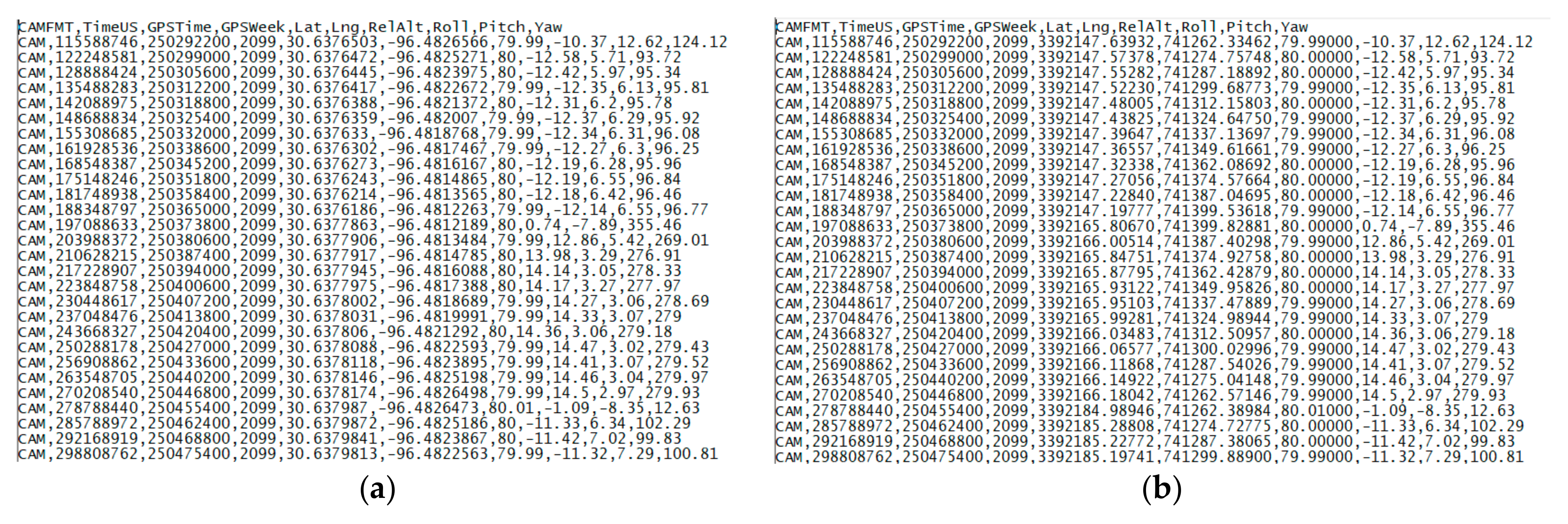
When a simulation run completed the mission, the flight log downloaded contained the status of the FCU recorded at 5 Hz throughout the flight. This led to a log containing 150,000 to 200,000 lines of information in each simulation run. For this study, the position and attitude of the craft at the time of image acquisition and the battery power consumed at the end of the mission were of particular interest. To meet the needs, a Python script that read the flight log and output a text file containing the desired information was written. The script looked for flight log messages beginning with the “CAM” tag (i.e., camera shutter information) and wrote them to a text file in a designated format. Then the script found the last flight log message containing a “BAT” tag (i.e., gathered battery data) and wrote it to a separate text file. The “CAM” messages contained the attitude and positional information of the airframe when the camera was triggered during the mission (Figure 4a). The position coordinates were recorded in the World Geodetic System 1984 (WGS-84) ellipsoidal model, and they were converted to the Universal Transverse Mercator (UTM) projected coordinate system to facilitate statistical analysis (Figure 4b) [41]. All altitudes were left in their original AGL format. The “BAT” message contained information on the total power consumed during the mission.

2.4. Data Aggregation and Statistical Metrics

The “CAM” and “BAT” files were imported into a master file in Microsoft Excel format to determine the wind impacts. The metrics used included average 3D error, standard deviation, flight time, and battery use.

The average 3D error and the standard deviation of 3D error provided metrics for the differences between intended waypoints and the corresponding camera trigger locations. The average 3D error in each individual simulation run is defined as

$$\overline{d}=\frac{{{\displaystyle \sum }}_{n=1}^m\Vert p_n-q_n\Vert }{m}$$

(3)

where $\overline{d}$ is the average 3D error between intended waypoints and actual camera trigger locations, $m$ is the number of waypoints where the camera was supposed to be triggered ($m=48$ and 96 in the single-altitude and dual-altitude cases, respectively), $p$ and $q$ are the intended waypoint location vector and corresponding actual camera trigger location vector, respectively, and $p-q$ is the 3D Euclidean distance.

The standard deviation in each individual simulation run can be expressed as

$$\sigma =\sqrt{\frac{{{\displaystyle \sum }}_{n=1}^m{\left(d_m-\overline{d}\right)}^2}{m-1}}$$

(4)

where $\sigma$ is standard deviation of 3D errors between intended waypoints and actual camera trigger locations, $m$ is the number of waypoints where the camera is supposed to be triggered, and $d_m$ is the 3D error between an intended waypoint and its associated camera trigger location.

Flight time provided a metric for the total time needed to complete a mission (i.e., from the first to the last image taken). Battery use provided a metric for the cumulative use of battery power.

3. Results

3.1. Simulation Runs for Single Altitude at 80 m AGL

3.1.1. Average 3D Error and Standard Deviation

As shown in

Table 4. Average 3D errors (m) between intended waypoints and actual camera trigger locations for 58 simulation runs at single altitude of 80 m AGL.

Wind Speed (m/s)	Wind Direction (°)
	0		22.5		45			67.5			90
Turbulence index = 0
0.0	0.19
3.5	0.19		0.19			0.20			0.19			0.19
7.0	0.19		0.19			0.20			0.19			0.20
10.5	0.19		0.20			0.20			0.21			0.24
14.0	0.24		0.34			0.66			0.71			0.66
Turbulence index = 5
10.5	0.26	0.26		0.26			0.28			0.30
Turbulence index = 10
0.0	0.26
3.5	0.27		0.28		0.27			0.27			0.25
7.0	0.36		0.36		0.33			0.37			0.39
10.5	0.55		0.56		0.45			0.53			0.53
Turbulence index = 20
0.0	0.66
3.5	0.67		0.62		0.56			0.60			0.54
7.0	0.78		0.9		0.71			0.80			0.83
10.5	1.25		1.28		1.36			1.21			1.09

, the average 3D error between intended waypoints and actual camera trigger locations increased as the wind speed increased. The magnitude of the impacts varied significantly as a function of the turbulence level. Specifically, as the turbulence level increased, the impact on the average 3D error became more noticeable. This observation is not surprising because the sUAS tried to compensate for the wind and stabilize its platform to where the waypoints were intended.

For low turbulence levels (i.e., turbulence indices of 0 and 5), the average 3D error did not increase significantly if the wind speed was up to 10.5 m/s. If the speed increased to 14 m/s, the 3D error was at least 26% higher compared to the average 3D error for the speed up to 10.5 m/s. For a turbulence index of 10, the average 3D error began to vary significantly at lower speeds. For instance, compared to the reference zero-speed with no-turbulence wind scenario, a 42% higher average 3D error was observed for a wind speed of 3.5 m/s. 89% and 189% higher values were observed for wind speeds of 7.0 m/s and 10.5 m/s, respectively. For a turbulence index of 20, the average 3D error began to vary at even lower speeds. For instance, compared to the reference zero-speed with no-turbulence wind scenario, the average 3D errors were found to be 253%, 311%, and 558% higher for wind speeds of 3.5 m/s, 7.0 m/s, and 10.5 m/s, respectively.

Based on the simulation runs, maximum average 3D error reached up to 1.36 m when wind speed was set to 10.5 m/s with a turbulence index of 20. This was the worst (i.e., most extreme) wind condition evaluated in the study that still allowed the simulated quadcopter to maintain travel along the planned mission route. Greater wind disturbance could be programmed in Mission Planner’s SITL. However, that would result in failed flight missions for the selected quadcopter model and divergent 3D errors.

In addition to displaying wind direction as shown in Table 4,

Table 5. Average 3D errors (m) between intended waypoints and actual camera trigger locations with respect to aircraft-wind angular relationship (i.e., α value) for 58 simulation runs at single altitude of 80 m AGL.

Wind Speed (m/s)	Aircraft-Wind Angular Relationship (i.e., α Value)
	α = 0° (Headwind)	α = 180° (Tailwind)	α = 90° (Crosswind)	α = 270° (Crosswind)	α = 67.5°	α = 247.5°	α = 45°	α = 225°	α = 22.5°	α = 202.5°
Turbulence index = 0
0.0	0.19
3.5	0.20	0.19	0.19	0.19	0.19	0.19	0.19	0.20	0.19	0.19
7.0	0.18	0.21	0.18	0.19	0.18	0.20	0.18	0.21	0.18	0.21
10.5	0.19	0.29	0.18	0.20	0.17	0.22	0.17	0.23	0.17	0.24
14.0	0.96	0.37	0.19	0.29	0.36	0.32	0.93	0.39	0.96	0.46
Turbulence index = 5
10.5	0.30	0.30	0.23	0.30	0.25	0.27	0.22	0.30	0.30	0.26
Turbulence index = 10
0.0	0.26
3.5	0.24	0.25	0.27	0.28	0.28	0.29	0.23	0.31	0.28	0.26
7.0	0.37	0.41	0.34	0.38	0.37	0.35	0.28	0.37	0.37	0.37
10.5	0.53	0.52	0.54	0.55	0.59	0.53	0.43	0.48	0.51	0.55
Turbulence index = 20
0.0	0.66
3.5	0.54	0.54	0.72	0.62	0.53	0.72	0.55	0.57	0.60	0.61
7.0	0.84	0.81	0.70	0.86	1.06	0.73	0.74	0.67	0.82	0.78
10.5	1.14	1.03	1.35	1.16	1.14	1.42	1.20	1.52	1.10	1.31

further investigates average 3D errors with respect to aircraft-wind angular relationship (i.e., α value) for all 58 simulation runs at single altitude of 80 m AGL and divides each run up into two separate segments that correspond to the East and West flight lines. For instance, the columns of “α = 180° (Tailwind)” and “α = 0° (Headwind)” together correspond to that of wind direction of 90° in Table 1. The columns of “α = 90° (Crosswind)” and “α = 270° (Crosswind)” together correspond to that of wind direction of 0° in Table 1. It is worth reiterating that the crosswind refers to the wind movement occurring perpendicular to the flight path. The columns of “α = 202.5°” and “α = 22.5°” together reflect the scenario where wind direction equated to 67.5° (Figure 3e,f).

For a turbulence index of 0, if the wind speed was up to 7.0 m/s, the variation in average 3D error due to differences in the α value was up to (0.21$-$0.18)$/$0.18 $=$ 17%. Compared to a reference zero-speed with no-turbulence wind scenario, the average 3D error varied from −5% to 11%. The impact was more noticeable as the wind speed increased. If the wind speed was 10.5 m/s, the variation in average 3D error due to differences in the α value was up to 64%. At 14 m/s, the variation in average 3D error due to differences in the α value was up to 405%.

For a turbulence index of 10, if the wind speed was up to 7.0 m/s, the variation in average 3D error due to differences in the α value was up to 69%. If the wind speed was 10.5 m/s, the variation in average 3D error due to differences in the α value was up to 85%.

For a turbulence index of 20, if the wind speed was up to 7.0 m/s, the variation in average 3D error due to differences in the α value was up to 205%. If the wind speed was 10.5 m/s, the variation in average 3D error due to differences in the α value was up to 258%.

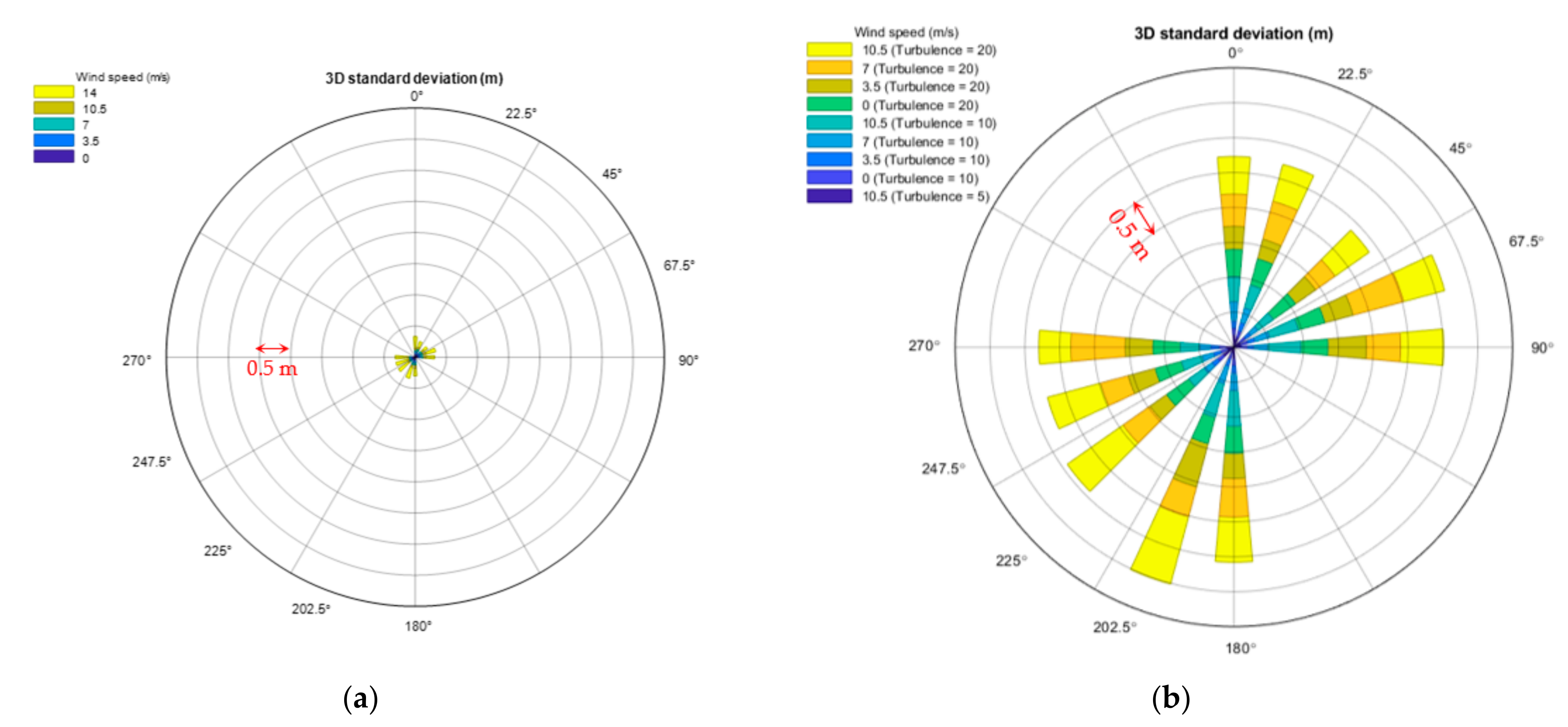
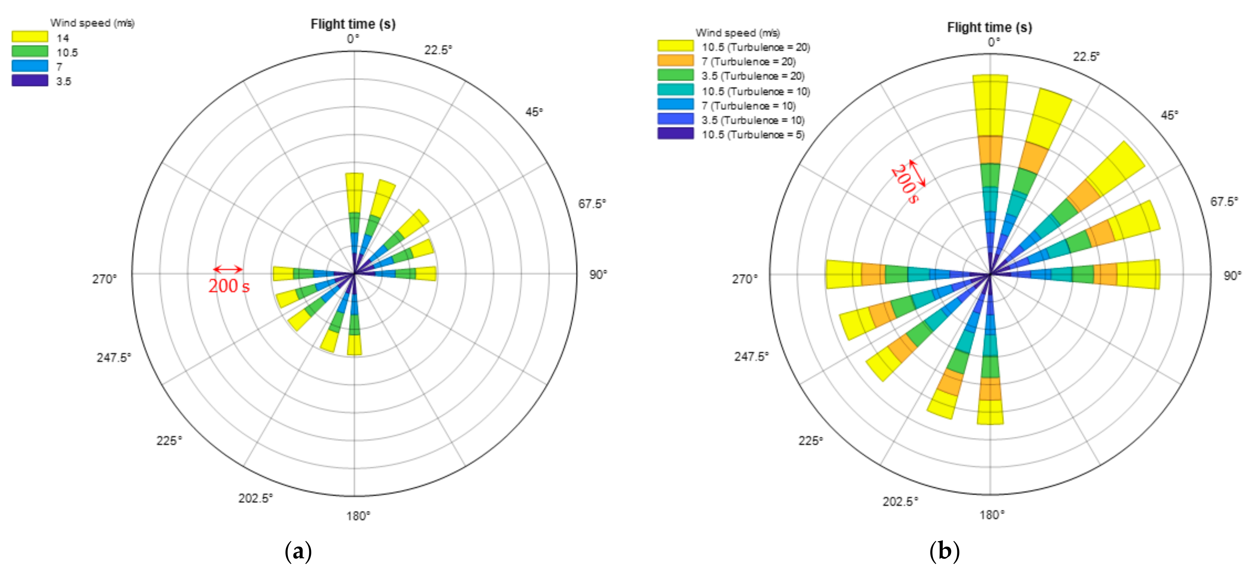
Figure 5 creates wind rose charts that give a view of how wind conditions impact average 3D error in all 58 simulation runs. Results display average 3D error without turbulence (Figure 5a) and that impacted by turbulence (Figure 5b). The angles written outside the circles depict the α angles. Each wind speed/turbulence scenario assigns a distinct color for representation. The radius of the wind rose reflects the magnitude of the average 3D error for a particular wind condition. Adjacent concentric circles have an interval of 0.5 m in radius.

Figure 5a suggests that when no turbulence was involved, least average 3D error was generated in crosswind scenarios, i.e., the aircraft and wind directions were perpendicular (i.e., α = 90° or 270°). Average 3D error tended to enlarge in all other scenarios where a headwind or tailwind component contributed during the flight mission. Observations in Figure 5a also reveal that pure headwind scenario (i.e., α = 0°) created worst flight stabilities and positional errors than any other scenarios when wind speed was up to 14 m/s (i.e., average 3D error was 0.96 m). Figure 5b demonstrates that when turbulence existed (i.e., turbulence index of 5, 10 or 20), average 3D error remarkably increased in all possible α values, indicating that average 3D error was less sensitive to the differences of aircraft-wind angular relationship than turbulence.

Table 6. Standard deviations (m) of 3D errors between intended waypoints and actual camera trigger locations for 58 simulation runs at single altitude of 80 m AGL.

Wind Speed (m/s)	Wind Direction (°)
	0		22.5		45			67.5			90
Turbulence index = 0
0.0	0.04
3.5	0.03		0.03			0.04			0.04			0.03
7.0	0.03		0.04			0.04			0.04			0.04
10.5	0.04		0.05			0.05			0.05			0.07
14.0	0.18		0.18			0.31			0.29			0.34
Turbulence index = 5
10.5	0.11	0.09		0.15			0.11			0.16
Turbulence index = 10
0.0	0.10
3.5	0.11		0.11		0.10			0.11			0.1
7.0	0.18		0.19		0.14			0.24			0.26
10.5	0.39		0.37		0.27			0.42			0.43
Turbulence index = 20
0.0	0.39
3.5	0.48		0.42		0.32			0.49			0.34
7.0	0.65		0.62		0.41			0.50			0.50
10.5	0.55		0.71		0.82			0.8			0.59

shows the standard deviation of 3D distance (i.e., 3D error) between intended waypoints and actual camera trigger locations for all 58 simulation runs at single altitude of 80 m AGL, and

Table 7. Standard deviations (m) of 3D errors between intended waypoints and actual camera trigger locations with respect to aircraft-wind angular relationship (i.e., α value) for 58 simulation runs at single altitude of 80 m AGL.

Wind Speed (m/s)	Aircraft-Wind Angular Relationship (i.e., α Value)
	α = 0° (Headwind)	α = 180° (Tailwind)	α = 90° (Crosswind)	α = 270° (Crosswind)	α = 67.5°	α = 247.5°	α = 45°	α = 225°	α = 22.5°	α = 202.5°
Turbulence index = 0
0.0	0.04
3.5	0.03	0.04	0.04	0.03	0.04	0.03	0.04	0.03	0.04	0.04
7.0	0.03	0.04	0.04	0.02	0.04	0.02	0.04	0.03	0.04	0.04
10.5	0.04	0.06	0.05	0.03	0.06	0.03	0.05	0.03	0.04	0.04
14.0	0.19	0.12	0.14	0.20	0.16	0.20	0.07	0.20	0.10	0.19
Turbulence index = 5
10.5	0.17	0.16	0.09	0.11	0.10	0.09	0.10	0.18	0.14	0.08
Turbulence index = 10
0.0	0.10
3.5	0.10	0.11	0.09	0.12	0.11	0.11	0.09	0.10	0.12	0.10
7.0	0.28	0.25	0.20	0.16	0.22	0.17	0.13	0.14	0.22	0.26
10.5	0.36	0.51	0.48	0.28	0.43	0.31	0.27	0.27	0.34	0.50
Turbulence index = 20
0.0	0.39
3.5	0.33	0.36	0.55	0.40	0.42	0.40	0.35	0.29	0.29	0.64
7.0	0.46	0.55	0.49	0.78	0.75	0.41	0.34	0.47	0.56	0.44
10.5	0.54	0.65	0.62	0.46	0.61	0.79	0.60	0.98	0.55	1.00

summarizes standard deviation with respect to aircraft-wind angular relationship. Figure 6 shows wind rose plots of standard deviations for all 58 simulation runs. Compared with wind impacts on average 3D error, similar conclusions can be drawn to the impacts on standard deviation.

3.1.2. Flight Time

Table 8. Total flight times (s) for 58 simulation runs at single altitude of 80 m AGL.

Wind Speed (m/s)	Wind Direction (°)
	0		22.5		45			67.5			90
Turbulence index = 0
0.0	318
3.5	318		318			318			318			318
7.0	318		318			318			318			318
10.5	319		318			318			318			319
14.0	358		359			416			448			456
Turbulence index = 5
10.5	320	323		325			325			325
Turbulence index = 10
0.0	320
3.5	320		320		320			323			321
7.0	322		323		323			326			324
10.5	339		341		344			357			356
Turbulence index = 20
0.0	351
3.5	360		346		357			353			362
7.0	377		374		390			391			397
10.5	635		635		665			635			657

shows total flight times (i.e., from the first image to the last image) for each simulation run at single altitude of 80 m AGL. In general, the total time to complete a mission was less sensitive to changes in wind speed, direction, and turbulence conditions than the average 3D error and standard deviation. If the wind speed was up to 7.0 m/s and the turbulence index was up to 10, the flight time increased approximately 2.5% compared to the reference zero-speed with no-turbulence wind simulation run. At this wind speed, even if the turbulence index was 20, the total flight time increased less than 25% compared to the reference zero-speed with no-turbulence simulation run. If the wind speed was 10.5 m/s and the turbulence index was up to 10, the total flight time increased approximately 12% compared to the reference zero-speed with no-turbulence wind simulation run. However, if the turbulence level was 20, the total flight time increased 109% compared to the reference zero-speed with no-turbulence run.

Table 9. Flight times (s) with respect to aircraft-wind angular relationship (i.e., α value) for 58 simulation runs at single altitude of 80 m AGL.

Wind Speed (m/s)	Aircraft-Wind Angular Relationship (i.e., α Value)
	α = 0° (Headwind)	α = 180° (Tailwind)	α = 90° (Crosswind)	α = 270° (Crosswind)	α = 67.5°	α = 247.5°	α = 45°	α = 225°	α = 22.5°	α = 202.5°
Turbulence index = 0
0.0	N/A
3.5	146	146	146	146	146	146	146	146	146	146
7.0	146	146	146	146	146	146	146	146	146	146
10.5	146	147	146	146	146	146	146	146	146	146
14.0	284	145	146	146	152	147	218	147	262	146
Turbulence index = 5
10.5	153	146	146	146	147	146	151	145	151	148
Turbulence index = 10
0.0	N/A
3.5	148	146	146	147	148	146	148	146	151	146
7.0	153	145	148	147	150	146	151	145	152	147
10.5	178	151	150	158	156	152	170	146	177	150
Turbulence index = 20
0.0	N/A
3.5	172	160	159	164	159	159	158	164	168	157
7.0	202	163	168	172	177	166	197	163	196	166
10.5	442	177	313	256	340	219	397	194	403	174

Note: This table excluded transit times between flight lines. This table did not include flight time information for all zero-speed simulation runs due to unavailability of the α angle.

shows flight times disaggregated by aircraft-wind angular relationship for all 58 simulation runs at single altitude of 80 m AGL. The time required to transit from the last waypoint of one flight line to the first waypoint of the next line was not included (i.e., 18.8 m as shown in Figure 1). If the wind speed was up to 7.0 m/s and the turbulence index was up to 10, the variation in flight time due to differences in aircraft-wind angular relationship (i.e., α value) was no greater than 6%. Unsurprisingly, headwind conditions produced a higher total flight time than tailwind conditions. The effect due to differences in aircraft-wind angular relationship was more noticeable for higher wind speeds and turbulence levels. If the wind speed was 10.5 m/s and the turbulence index was 10, the total flight time was 18% greater under headwind condition than under tailwind condition. However, if the wind speed was 14 m/s and the turbulence index was 20, the total flight time was 182% higher under headwind condition than under tailwind condition. In Table 9, it is worth nothing that “N/A” was marked as flight times for zero-wind-speed simulation runs where the aircraft-wind angular relationships were not formed. The directionality of wind impacts on flight times is also quantified in the wind rose plots in Figure 7.

3.1.3. Battery Use

Similar to analysis performed with the flight time metric, battery use (

Table 10. Battery use (mAh) for 58 simulation runs at single altitude of 80 m AGL.

Wind Speed (m/s)	Wind Direction (°)
	0		22.5		45			67.5			90
Turbulence index = 0
0.0	2601
3.5	2661		2660			2660			2659			2659
7.0	2917		2910			2915			2921			2928
10.5	3214		3212			3217			3220			3224
14.0	3874		3883			4377			4707			4774
Turbulence index = 5
10.5	3233	3177		3188			3206			3274
Turbulence index = 10
0.0	2572
3.5	2644		2639		2643			2657			2658
7.0	2953		2955		2943			2970			2952
10.5	3385		3323		3339			3511			3492
Turbulence index = 20
0.0	2726
3.5	2904		2816		2865			2941			2893
7.0	3248		3219		3411			3413			3483
10.5	5537		5641		5849			5746			5822

) was also less sensitive to changes in wind speed, direction, and turbulence conditions than the average 3D error and standard deviation. If the wind speed was up to 7.0 m/s and the turbulence index was up to 10, the flight time increased less than 14% compared to the reference zero-speed with no-turbulence simulation run. At this wind speed, even if the turbulence index was 20, the total battery use increased less than 34% compared to the reference zero-speed with no-turbulence run. If the wind speed was up to 10.5 m/s and the turbulence index was up to 10, the battery use increased less than 35% compared to the reference zero-speed with no-turbulence run. However, if the turbulence level was 20, the battery use increased 125%.

3.2. Simulation Runs for Dual Altitudes at 80 m and 10 m AGL

As displayed in Table 3, the simulation included a wind speed of 10.5 m/s with two possible turbulence index values of 0 and 10 at 80 m AGL, and the simulation also included a wind speed of 3.5 m/s with a turbulence index of 0 at 10 m AGL. These were evaluated at three wind directions resulting in a total of six simulation runs taking into account both the 80 m and 10 m AGL flight paths per a simulation as shown in Figure 2.

Table 11. Evaluation results for six simulation runs at dual altitudes of 80 m and 10 m AGL. Each value indicates the evaluation result that took both 80 m and 10 m AGL into account.

Evaluation Metric	Wind Direction (°)
	0	45	90
Turbulence index = 0 at both 10 m and 80 m AGL
Average 3D error (m)	0.20	0.21	0.23
Standard deviation (m)	0.05	0.05	0.06
Total flight time (s)	473	471	473
Battery use (mAh)	4418	4418	4425
Turbulence index = 0 at 10 m, turbulence index = 10 at 80 m AGL
Average 3D error (m)	0.38	0.34	0.37
Standard deviation (m)	0.33	0.23	0.35
Total flight time (s)	494	497	509
Battery use (mAh)	4590	4539	4693

Note: The total flight time values in the table excluded transit times from 80 m descending to 10 m AGL.

summarizes evaluation results for the six simulation runs. Each value in the table indicates the evaluation result that took both 80 m and 10 m AGL into account. When no turbulence was involved at both 80 m and 10 m AGL, each evaluation metric was found to vary slightly between scenarios with different wind directions. The average 3D error and standard deviation statistics were consistent with that reported in Table 4 and Table 6 when looking into the cells with a turbulence index of 0 and wind speed of 10.5 m/s. This emphasizes that the choice of flight height will not affect simulated wind impacts on flight performance as stated in Section 2.1. However, the flight endurance and battery use in Table 11 increased compared with that reported in Table 8 and Table 10 when looking into the cells with a turbulence index of 0 and wind speed of 10.5 m/s. This is because Table 11 involved dual altitudes in the mission. Compared with the scenario where the turbulence index was 0 at both 10 m and 80 m AGL, when the turbulence index was increased up to 10 at 80 m AGL, the average 3D error and standard deviation values were found to increase significantly while the total flight time and battery use were observed to rise by up to 7.6% and 6.1%, respectively (Table 11).

Table 12. Evaluation results with respect to aircraft-wind angular relationship (i.e., α value) for six simulation runs at dual altitudes of 80 m and 10 m AGL. Each value indicates the evaluation result that took both 80 m and 10 m AGL into account.

Evaluation Metric	Aircraft-Wind Angular Relationship (i.e., α Value)
	α = 0° (Headwind)	α = 180° (Tailwind)	α = 90° (Crosswind)	α = 270° (Crosswind)	α = 45°	α = 225°
Turbulence index = 0 at both 10 m and 80 m AGL
Average 3D error (m)	0.21	0.25	0.19	0.21	0.19	0.23
Standard deviation (m)	0.05	0.07	0.06	0.04	0.05	0.04
Flight time (s)	212	213	212	212	212	212
Turbulence index = 0 at 10 m AGL and turbulence index = 10 at 80 m AGL
Average 3D error (m)	0.38	0.36	0.37	0.38	0.32	0.35
Standard deviation (m)	0.30	0.39	0.38	0.26	0.22	0.23
Flight time (s)	244	218	216	224	236	212

Note: The total flight time values in the table excluded transit times from 80 m descending to 10 m AGL. The flight time values in the table also excluded transit times between flight lines.

shows evaluation results with respect to aircraft-wind angular relationship (i.e., α value) for the six simulation runs at dual altitudes of 80 m and 10 m AGL. Each value indicates the evaluation result that took both 80 m and 10 m AGL into account. Similar to observations in Section 3.1.1, when turbulence existed at 80 m AGL (i.e., turbulence index of 10), flight stability remarkably decreased in all possible α values compared to the no-turbulence scenarios indicating that average 3D error and standard deviation were more sensitive to turbulence than the differences of aircraft-wind angular relationship.

Different from Table 12, each value in

Table 13. Evaluation results with respect to aircraft-wind angular relationship (i.e., α value) for six simulation runs at dual altitudes of 80 m and 10 m AGL. This table shows disaggregated results by considering partial flight operation conducted at each altitude (i.e., either 80 m or 10 m AGL) separately.

Evaluation Metric	Aircraft-Wind Angular Relationship (i.e., α Value)
	α = 0° (Headwind)	α = 180° (Tailwind)	α = 90° (Crosswind)	α = 270° (Crosswind)	α = 45°	α = 225°
Turbulence index = 0 at 80 m AGL
Average 3D error (m)	0.19	0.29	0.18	0.20	0.17	0.23
Standard deviation (m)	0.04	0.06	0.05	0.03	0.05	0.03
Flight time (s)	146	147	146	146	146	146
Turbulence index = 10 at 80 m AGL
Average 3D error (m)	0.53	0.52	0.54	0.55	0.43	0.48
Standard deviation (m)	0.36	0.51	0.48	0.28	0.27	0.27
Flight time (s)	178	151	150	158	170	146
Turbulence index = 0 at 10 m AGL
Average 3D error (m)	0.22	0.20	0.19	0.21	0.22	0.22
Standard deviation (m)	0.05	0.04	0.07	0.05	0.05	0.04
Flight time (s)	66	66	67	67	66	66

Note: The total flight time values in the table excluded transit times from 80 m descending to 10 m AGL. The flight time values in the table also excluded transit times between flight lines.

indicates the disaggregated evaluation result that considered partial flight operation conducted at each altitude (i.e., either 80 m or 10 m AGL) separately. Expectedly, the worst flight performance was achieved when the turbulence index was up to 10 at 80 m AGL. However, when no turbulence was involved, nearly identical flight performances were obtained between the 80 m and 10 m AGL simulation scenarios in terms of the average 3D error and standard deviation. This is because the flight height in the study is independent to simulated wind effects and, therefore, the choice of flight height will not affect wind impacts as explained earlier in Section 2.1. On the other hand, the flight time at 10 m AGL was decreased remarkably compared to that at 80 m AGL for any given α angle. This is because the flight lines were scaled down at 10 m AGL as shown in Figure 2.

4. Lessons Learned and Conclusion

A timely investigation and reconstruction at the motor vehicle crash scene plays a pivotal role in identifying the cause and severity of the accident, assessing roadway safety risks, clarifying insurance liabilities, and facilitating legal proceedings. SfM photogrammetry with sUAS in crash scene reconstruction has gained increasing attention in recent years because of its reliability and flexibility in offering quality geospatial surveying products. One of the main deficiencies in past literature has been the failure of demonstrating its effectiveness in adverse weather conditions, under which the risk of motor vehicle crashes is exacerbated. In this article, wind was chosen as the primary factor that drove adverse weather conditions, and the sUAS was presented in the form of a simulated quadcopter in the ArduPilot SITL environment. The main objectives were to: (1) characterize the impacts of wind speed, direction, and turbulence on the positional accuracy, required flight time, and battery use of the simulated quadcopter type via realistic flight simulations, and (2) generalize lessons learned for platform-independent quadcopter flight design under wind conditions for crash scene mapping. Real-world quadcopters were not tested and compared due to flight safety and compliance concerns. The simulation also provided a method to assess wind impact on flight design in a systematic and controlled fashion, which is generally not feasible in real-world operating conditions. A total of 58 simulation runs with incremental increases in wind speed, direction, and turbulence were created and analyzed at a single altitude of 80 m AGL. Six more simulation runs were created and analyzed at dual altitudes of 80 m and 10 m AGL.

The wind disturbance settings were deliberately chosen to ensure that the simulated quadcopter was able to maintain the planned route and avoid divergent 3D errors between intended waypoints and actual camera trigger locations. The results indicated that as wind conditions departed from the ideal zero-speed with no-turbulence scenario, there was an adverse impact on sUAS stability performance, measured in terms of positional accuracy, required flight time, and battery use. Several lessons learned related to real-world quadcopter sUAS flight design under wind conditions for crash scene reconstruction are discussed and summarized below.

The average 3D error and corresponding standard deviation of 3D error between planned waypoints and the actual camera trigger locations increased as the wind speed increased. The research findings suggested operating the simulated quadcopter when the wind is not greater than 11 m/s. It is important to note that this ArduPilot quadcopter module has been run on real-world systems such as 3DR Solo and Parrot Bebop 2, and this conclusion accords well with the accepted wind tolerance that the respective user guides recommend for these platforms [33,34,42]. This recommendation on wind tolerance is also consistent with that of other popular quadcopter sUAS platforms in current operation of similar size such as DJI Phantom 4 Pro/Pro+, DJI Inspire 2 and Skydio 2 [43,44,45]. However, it should be realized that wind tolerance is platform dependent and 11 m/s as the documented value in this work may not be generalized for all types of quadcopter sUAS platforms. For the average 3D error and corresponding standard deviation of 3D error between planned waypoints and the actual camera trigger locations, the magnitude of the impact varied significantly as a function of the turbulence level. The simulation runs also demonstrated that the flight performance remained relatively stable under light to moderate turbulence levels (i.e., turbulence level ≤5).

Flying perpendicular to the wind direction is a well-known practice for fixed-wing sUAS survey missions. It helps maintain stable ground speed during imagery data collection [46,47]. Results obtained in this study suggest that this rule of thumb for fixed-wing aircrafts applies well to quadcopter sUAS platforms. Under high wind and low turbulence scenarios (e.g., a wind speed of 14 m/s and turbulence level of 0), statistical results proved that flying in crosswind (i.e., α = 90° or 270°) and against headwind (i.e., α = 0°) were the most and least favorable flight patterns, respectively. While the average 3D error metric was not sensitive to the increase of wind speed in crosswind scenarios (i.e., α = 90° or 270°), the average 3D error sharply grew four times if wind speed rose from 0 to 14 m/s for the headwind scenario (i.e., α = 0°). Similar results were observed in the flight time metric. The sUAS spent nearly twice as much time on headwind flight segments (i.e., α = 0°) than those segments where flight lines were perpendicular to the wind direction (i.e., α = 90° or 270°). As shown in the simulation runs, the total flight time metric was less sensitive to changes in wind speed, direction, and turbulence conditions than the average 3D error and standard deviation metrics. The ideal flight paths for quadcopter sUAS platforms are, therefore, supposed to stay nearly perpendicular to horizontal wind. However, in real-world scenarios, this goal may not be achievable in every single flight attempt due to road geometry at the crash location, overhead safety concerns, airspace restrictions and so forth. A general recommendation to the crash investigation team and sUAS remote pilot within high wind and low turbulence environments is to apply this conclusion when pertinent on-site conditions permit.

Under strong wind conditions (e.g., wind speed ≥ 11 m/s and turbulence level >5 for the simulated quadcopter platform in ArduPilot SITL), flight stability degraded dramatically, resulting in disrupted frontal and side overlap settings due to large waypoint targeting errors. This overlap disruption is expected to get amplified for flight missions at a low altitude (e.g., below 10 m AGL) due to smaller camera field of view (FOV). This can result in a decreased number of detected and matched features in a pair of overlapping images in SfM processing routine, potentially affecting the overall quality of 2D orthomosaic image and 3D point cloud products. Even if overlaps are not disrupted in some cases, remote pilots are supposed to take battery usage into careful consideration prior to conducting high-wind flight missions. Nowadays, many commercially available multirotor sUAS platforms need a 2S to 6S lithium-ion polymer (LiPo) battery with the energy capacity less than 6000 mAh to achieve best balance between performance, flight time, and weight [43,44,45,48,49]. Assuming this battery specification applies to the examined quadcopter platform in ArduPilot SITL, Table 10 implies that when strong wind and turbulence exist (i.e., wind speed of 10.5 m/s and turbulence level of 20), the fully charged LiPo battery can potentially run out of power before completion of the mapping mission over the simulated crash scene area of 105 × 70 m. The rapid degradation in flight efficiency as observed from the simulation runs and platform demonstrates the need for adequate battery backup under high wind conditions, even when the scene is within a limited geographic extent. However, while this statement is generalized, it needs to be pointed out that battery consumption is platform dependent. Some lighter weight quadcopters may potentially complete a mission with one LiPo battery should they withstand as much wind as the simulated quadcopter type.

At a crash scene, the quadcopter to be deployed on the ground usually stay in close proximity to the on-site investigators and nearby vehicles. If the wind speed is marginally below the aforementioned maximum wind tolerance (e.g., 11 m/s for the simulated quadcopter in ArduPilot SITL), the remote pilot is supposed to pay extra attention during quadcopter take-off and landing phases. This is because a quadcopter sUAS is likely more susceptible to the air movement when it is flat on the ground and sitting still, causing an increased risk of flipping over in windy conditions. When the platform comes to hover in the air or traverse pre-defined waypoints to collect images for a photogrammetric survey, it should largely be able to withstand the maximum wind tolerance in a relatively steady state. In such phase, the gimbal stabilizer, which is nowadays attached to many commercially available quadcopter sUAS platforms, also helps maintain favorable image quality by compensating for angular motions to the onboard camera.

It is worth emphasizing that as a popular and reliable open-source autopilot software suite, ArduPilot has been used on a wide spectrum of autonomous systems with full-featured autonomous capabilities. ArduPilot on SITL features a high-fidelity simulation environment running a realistic flight dynamics model, and therefore, the major simulation findings summarized in this study are expected to be applicable to real-world flight scenarios. In addition, the choice of 80 m and 10 m AGL in the article was generic. Changing flight altitude did not vary wind and turbulence effect and hence, did not affect the simulated results other than flight endurance and battery consumption. The wind and turbulence parameters were defined and adjusted in Mission Planner interface, so the same wind impact results apply to other pre-defined flight altitude for the simulated quadcopter without loss of generality. However, in a real-world flight mission for crash scene reconstruction, flight height is usually determined by considering factors such as desired GSD and camera model settings, flight time, geographic extent of the mission, and waypoint geometry given specific overlap settings.

In the United States, public and commercial sUAS operations within the national airspace system (NAS) require obtaining either a Certificate of Waiver or Authorization (COA), with the option of including a Section 333 exemption, or Part 107 license from the Federal Aviation Administration (FAA). For public safety and transportation agencies that administer auto crash investigation, having a COA may warrant sUAS operations across vast airspace regions. More importantly, the COA may grant these agencies privilege of flying in suboptimal flight conditions, such as during nighttime and foggy hours to carry out an emergency survey immediately after a crash takes place. On the other hand, getting a Part 107 license usually requires less time and effort, but it is generally considered more restrictive in various dimensions compared with the COA. Thanks to the FAA’s recent efforts, waivers to Part 107 rules can be applied to gain approvals of certain sUAS operations outside the limitations defined in the rules [50]. For example, a waiver can request easing the restrictions of conducting routine sUAS operations above standard Part 107 flight height limits (e.g., 121.9 m (400 ft) AGL at the time of this writing). This type of special permission allows pilots of public safety and transportation agencies to operate sUASs with adequate flexibility at a crash scene while ensuring safety and compliance. Recently, the FAA provided rule amendments to Part 107 to enable routine operations of sUAS over people, from moving vehicles, and at night under certain conditions. Nowadays, sUASs have become an integral part of our daily life, and technologies to advance sUAS safety evolve rapidly. This leaves open the possibilities of exploring impacts of multiple suboptimal weather conditions on sUAS flight performance for crash scene reconstruction in the near future. The intended future work also includes: 1) investigating wind impacts on fixed-wing sUAS platforms, and 2) conducting real-world flight missions with different commercially available quadcopters under varying wind conditions and assessing the flight performance as well as SfM photogrammetric products.

References

- Li, X.; Khattak, A.J.; Wali, B. Role of multiagency response and on-scene times in large-scale traffic incidents. Transp. Res. Rec. 2017, 2616, 39–48. [Google Scholar] [CrossRef] [Green Version]
- Agent, K.R.; Pigman, J.G. Traffic Accident Investigation (Report No. KTC-93-10); Kentucky Transportation Center-University of Kentucky: Lexington, KY, USA, 1993. [Google Scholar]
- Jacobson, L.N.; Legg, B.; O’Brien, A. Incident Management using Total Stations; Report No. WA-RD 284.1; Washington State Department of Transportation: Olympia, WA, USA, 1992. [Google Scholar]
- Duignan, P.; Griffiths, M.; Lie, A. Photogrammetric Methods in Crash Investigation. In Proceedings of the 15th International Technical Conference on Enhanced Safety of Vehicles, Melbourne, Australia, 13–26 May 1996. [Google Scholar]
- Forman, P.; Parry, I. Rapid Data Collection at Major Incident Scenes using Three Dimensional Laser Scanning Techniques. In Proceedings of the IEEE 35th Annual 2001 International Carnahan Conference on Security Technology, London, UK, 16–19 October 2001. [Google Scholar]
- Pagounis, V.; Tsakiri, M.; Palaskas, S.; Biza, B.; Zaloumi, E. 3D Laser Scanning for Road Safety and Accident Reconstruction. In Proceedings of the XXIIIth international FIG Congress, Munich, Germany, 8–13 October 2006. [Google Scholar]
- James, W.; McKinzie, S.; Benson, W.; Heise, C. Crash Investigation and Reconstruction Technologies and Best Practices; Report No.FHWA-HOP-16-009; U.S. Department of Transportation: Washington, DC, USA, 2015. [Google Scholar]
- Stevens, C.R.; Blackstock, T. Demonstration of Unmanned Aircraft Systems Use for Traffic Incident Management (UAS-TIM); Report No. PRC 17-69 F; Texas A&M Transportation Institute: College Station, TX, USA, 2017. [Google Scholar]
- John Hopkins University. Operational Evaluation of Unmanned Aircraft Systems for Crash Scene Reconstruction; Report No. AOS-17-0078; National Institute of Justice: Washington, DC, USA, 2017. [Google Scholar]
- Khan, M.A.; Ectors, W.; Bellemans, T.; Janssens, D.; Wets, G. Unmanned aerial vehicle-based traffic analysis: A case study for shockwave identification and flow parameters estimation at signalized intersections. Remote Sens. 2018, 10, 458. [Google Scholar] [CrossRef] [Green Version]
- Kamnik, R.; Perc, M.N.; Topolšek, D. Using the scanners and drone for comparison of point cloud accuracy at traffic accident analysis. Accid. Anal. Prev. 2020, 135, 105391. [Google Scholar] [CrossRef] [PubMed]
- Pérez, J.A.; Gonçalves, G.R.; Rangel, J.M.G.; Ortega, P.F. Accuracy and effectiveness of orthophotos obtained from low cost UASs video imagery for traffic accident scenes documentation. Adv. Eng. Softw. 2019, 132, 47–54. [Google Scholar] [CrossRef]
- How Do Weather Events Impact Roads? Available online: https://ops.fhwa.dot.gov/weather/q1_roadimpact.htm (accessed on 30 April 2021).
- Young, R.K.; Liesman, J. Intelligent transportation systems for operation of roadway segments in high-wind conditions. Transp. Res. Rec. 2007, 2000, 1–7. [Google Scholar] [CrossRef]
- Naik, B.; Tung, L.W.; Zhao, S.; Khattak, A.J. Weather impacts on single-vehicle truck crash injury severity. J. Saf. Res. 2016, 58, 57–65. [Google Scholar] [CrossRef] [PubMed]
- Slocum, R.K.; Wright, W.; Parrish, C.; Costa, B.; Sharr, M.; Battista, T.A. Guidelines for Bathymetric Mapping and Orthoimage Generation using sUAS and SfM: An Approach for Conducting Nearshore Coastal Mapping; NOAA Technical Memorandum: Silver Spring, MD, USA, 2019. [Google Scholar]
- Joyce, K.E.; Duce, S.; Leahy, S.M.; Leon, J.; Maier, S.W. Principles and practice of acquiring drone-based image data in marine environments. Mar. Freshw. Res. 2019, 70, 952–963. [Google Scholar] [CrossRef]
- Ding, L.; Wang, Z. A robust control for an aerial robot quadrotor under wind gusts. J. Robot. 2018, 2018, 5607362. [Google Scholar] [CrossRef] [Green Version]
- Ware, J.; Roy, N. An Analysis of Wind Field Estimation and Exploitation for Quadrotor Flight in the Urban Canopy Layer. In Proceedings of the 2016 IEEE International Conference on Robotics and Automation (ICRA), Stockholm, Sweden, 16–21 May 2016. [Google Scholar]
- Stepanyan, V.; Krishnakumar, K. Estimation, Navigation and Control of Multi-Rotor Drones in an Urban Wind Field. In Proceedings of the AIAA Information Systems-AIAA Infotech @ Aerospace, Grapevine, TX, USA, 9–13 January 2017. [Google Scholar]
- Wang, J.Y.; Luo, B.; Zeng, M.; Meng, Q.H. A wind estimation method with an unmanned rotorcraft for environmental monitoring tasks. Sensors 2018, 18, 4504. [Google Scholar] [CrossRef] [PubMed] [Green Version]
- Wang, B.H.; Wang, D.B.; Ali, Z.A.; Ting, B.T.; Wang, H. An overview of various kinds of wind effects on unmanned aerial vehicle. Meas. Control 2019, 52, 731–739. [Google Scholar] [CrossRef]
- Siqueira, J. Modeling of Wind Phenomena and Analysis of Their Effects on UAV Trajectory Tracking Performance. Master’s Thesis, West Virginia University, Morgantown, WV, USA, 2017. [Google Scholar]
- Biradar, A.S. Wind Estimation and Effects of Wind on Waypoint Navigation of UAVs. Master’s Thesis, Arizona State University, Tempe, AZ, USA, 2014. [Google Scholar]
- Yoon, S.; Shin, D.; Choi, Y.; Park, K. Development of a flexible and expandable UTM simulator based on open sources and platforms. Aerospace 2021, 8, 133. [Google Scholar] [CrossRef]
- Koubaa, A.; Allouch, A.; Alajlan, M.; Javed, Y.; Belghith, A.; Khalgui, M. Micro air vehicle link (mavlink) in a nutshell: A survey. IEEE Access 2019, 7, 87658–87680. [Google Scholar] [CrossRef]
- Baidya, S.; Shaikh, Z.; Levorato, M. FlyNetSim: An Open Source Synchronized UAV Network Simulator based on ns-3 and Ardupilot. In Proceedings of the 21st ACM International Conference on Modeling, Analysis and Simulation of Wireless and Mobile Systems (MSWiM’18), Montréal, QC, Canada, 28 October–2 November 2018. [Google Scholar]
- Eyerman, J.; Mooring, B.; Catlow, M.; Datta, S.; Akella, S. Low-Light Collision Scene Reconstruction Using Unmanned Aerial Systems; North Carolina Department of Transportation: Raleigh, NC, USA, 2018. [Google Scholar]
- Transforming Accident Investigation with Drones. Available online: https://medium.com/aerial-acuity/transforming-accident-investigation-with-drones-edec7162d8ce (accessed on 1 June 2021).
- Police Use of Unmanned Aircraft Systems (sUAS). Available online: http://records.tukwilawa.gov/weblink/1/edoc/285955/TIC%202017-02-28%20Item%202D%20-%20Discussion%20-%20Police%20Use%20of%20Unmanned%20Aircraft%20Systems%20 (accessed on 1 June 2021).
- Montgomery, K. Documenting Vehicle Crashes with Drone Photogrammetry. Available online: https://www.evidencemagazine.com/index.php?option=com_content&task=view&id=2437&Itemid=49 (accessed on 7 July 2021).
- Dukowitz, Z. Drones in Accident Reconstruction: How Drones Are Helping Make Traffic Crash Site Assessments Faster, Safer, and More Accurate. Available online: https://uavcoach.com/drones-accident-reconstruction/ (accessed on 7 July 2021).
- Solo User Manual V9; 3D Robotics Inc: Berkeley, CA, USA, 2015.
- Parrot Bebop Autopilot. Available online: https://ardupilot.org/copter/docs/parrot-bebop-autopilot.html (accessed on 1 June 2021).
- ArduPilot Complete Parameter List. Available online: https://ardupilot.org/copter/docs/parameters.html (accessed on 30 April 2021).
- Javadnejad, F.; Slocum, R.K.; Gillins, D.T.; Olsen, M.J.; Parrish, C.E. Dense point cloud quality factor as proxy for accuracy assessment of image-based 3D reconstruction. J. Surv. Eng. 2021, 147, 04020021. [Google Scholar] [CrossRef]
- Mölg, N.; Bolch, T. Structure-from-motion using historical aerial images to analyse changes in glacier surface elevation. Remote Sens. 2017, 9, 1021. [Google Scholar] [CrossRef] [Green Version]
- Turbulence—The Definitive Edition. Available online: https://www.weather.gov/media/zhu/ZHU_Training_Page/turbulence_stuff/turbulence2/turbulence.pdf (accessed on 30 April 2021).
- ArduPilot SIM_Aircraft.cpp Source Code. Available online: https://github.com/ArduPilot/ardupilot/blob/master/libraries/SITL/SIM_Aircraft.cpp (accessed on 30 April 2021).
- Seregina, L.S.; Haas, R.; Born, K.; Pinto, J.G. Development of a wind gust model to estimate gust speeds and their return periods. Tellus A: Dyn. Meteorol. Oceanogr. 2014, 66, 22905. [Google Scholar] [CrossRef] [Green Version]
- NOAA Vertical Datum Transformation. Available online: https://vdatum.noaa.gov/ (accessed on 30 April 2021).
- Parrot Bebop 2 Drone User Guide; Parrot SA: Paris, France, 2016.
- DJI Phantom 4 Pro/Pro+ Series User Manual; SZ DJI Technology Co., Ltd.: Shenzhen, China, 2020.
- DJI Inspire 2 User Manual; SZ DJI Technology Co., Ltd: Shenzhen, China, 2016.
- Skydio 2 User Guide; Skydio Inc: Redwood City, CA, USA, 2019.
- Chu, T.; Starek, M.J.; Brewer, M.J.; Murray, S.C.; Pruter, L.S. Assessing lodging severity over an experimental maize (Zea mays L.) field using UAS images. Remote Sens. 2017, 9, 923. [Google Scholar] [CrossRef] [Green Version]
- Chu, T.; Starek, M.J.; Brewer, M.J.; Murray, S.C.; Pruter, L.S. Characterizing canopy height with UAS structure-from-motion photogrammetry—results analysis of a maize field trial with respect to multiple factors. Remote Sens. Lett. 2018, 9, 753–762. [Google Scholar] [CrossRef] [Green Version]
- DJI Mavic 2 Pro/Zoom User Manual; SZ DJI Technology Co., Ltd.: Shenzhen, China, 2018.
- Parrot ANAFI Drone User Guide v2.6.2; Parrot SA: Paris, France, 2019.
- Operations of Small Unmanned Aircraft over People. Available online: https://www.faa.gov/news/media/attachments/OOP_Final%20Rule.pdf (accessed on 12 July 2021).
Figure 1.
Overview of flight lines and waypoints of the simulated crash scene within Mission Planner.
Figure 2.
Flight path for dual altitudes of 80 m and 10 m AGL. The simulated flight started the mission at 80 m AGL and then descended to continue the mission at 10 m AGL. The red arrows indicate flight courses. 80% frontal and 80% side overlap settings remained at both 80 m and 10 m AGL. There were 48 images taken at each AGL level.
Figure 3.
Examples of α angles when an aircraft does not fly in headwind, tailwind or crosswind. (a) α = 67.5° when wind direction is 22.5° and flight course is East. (b) α = 247.5° when wind direction is 22.5° and flight course is West. (c) α = 45° when wind direction is 45° and flight course is East. (d) α = 225° when wind direction is 45° and flight course is West. (e) α = 22.5° when wind direction is 67.5° and flight course is East. (f) α = 202.5° when wind direction is 67.5° and flight course is West.
Figure 4.
A section of flight log downloaded in a simulation run. (a) Original flight log; (b) Flight log after coordinate conversion to the UTM system.
Figure 5.
Wind rose plots of average 3D errors between intended waypoints and actual camera trigger locations at single altitude of 80 m AGL. (a) Wind rose plot of average 3D errors for no-turbulence runs; (b) Wind rose plot of average 3D errors for all simulation runs with turbulence.
Figure 6.
Wind rose plots of standard deviation of 3D errors between intended waypoints and actual camera trigger locations at single altitude of 80 m AGL. (a) Wind rose plot of standard deviations for no-turbulence runs; (b) Wind rose plot of standard deviations for all simulation runs with turbulence.
Figure 7.
Wind rose plots of total flight time at single altitude of 80 m AGL. (a) Wind rose plot of flight times for no-turbulence runs; (b) Wind rose plot of flight times for all simulation runs with turbulence.