U-Net Segmented Adjacent Angle Detection (USAAD) for Automatic Analysis of Corneal Nerve Structures
by
 ,
,
Philip Mehrgardt
1, 
Seid Miad Zandavi
1,
Simon K. Poon
1,
Juno Kim
2,
Maria Markoulli
2 and
Matloob Khushi
1,*
1
School of Computer Science, The University of Sydney, NSW 2006, Australia
2
School of Optometry and Vision Science, University of New South Wales, Sydney, NSW 2052, Australia
*
Author to whom correspondence should be addressed.
Data 2020, 5(2), 37; https://doi.org/10.3390/data5020037
Submission received: 20 February 2020
/
Revised: 4 April 2020
/
Accepted: 8 April 2020
/
Published: 14 April 2020
(This article belongs to the Special Issue Data-Driven Healthcare Tasks: Tools, Frameworks, and Techniques)
Abstract
:Measurement of corneal nerve tortuosity is associated with dry eye disease, diabetic retinopathy, and a range of other conditions. However, clinicians measure tortuosity on very different grading scales that are inherently subjective. Using in vivo confocal microscopy, 253 images of corneal nerves were captured and manually labelled by two researchers with tortuosity measurements ranging on a scale from 0.1 to 1.0. Tortuosity was estimated computationally by extracting a binarised nerve structure utilising a previously published method. A novel U-Net segmented adjacent angle detection (USAAD) method was developed by training a U-Net with a series of back feeding processed images and nerve structure vectorizations. Angles between all vectors and segments were measured and used for training and predicting tortuosity measured by human labelling. Despite the disagreement among clinicians on tortuosity labelling measures, the optimised grading measurement was significantly correlated with our USAAD angle measurements. We identified the nerve interval lengths that optimised the correlation of tortuosity estimates with human grading. We also show the merit of our proposed method with respect to other baseline methods that provide a single estimate of tortuosity. The real benefit of USAAD in future will be to provide comprehensive structural information about variations in nerve orientation for potential use as a clinical measure of the presence of disease and its progression.
1. Introduction
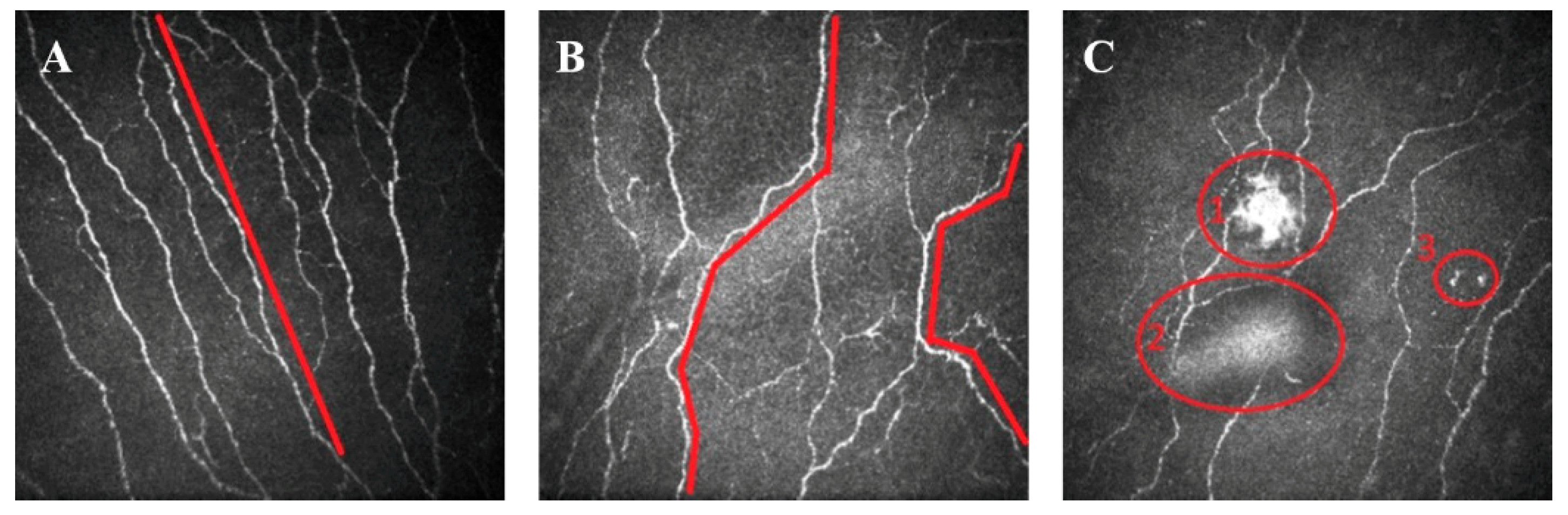
Corneal nerve tortuosity is a morphological property which indicates the degree of curvature in nerves found in the sub-basal nerve plexus of the cornea. Nerves with low tortuosity (Figure 1A) appear approximately straight, while high tortuosity nerves have many twists and are significantly curved (Figure 1B). Figure 1C shows other anomalies, such as washout, buckling and dendritic cells. Although these anomalies are not evaluated in the scope of this paper, they provide an enduring challenge to developing image analysis tools for clinical assessment of the cornea.
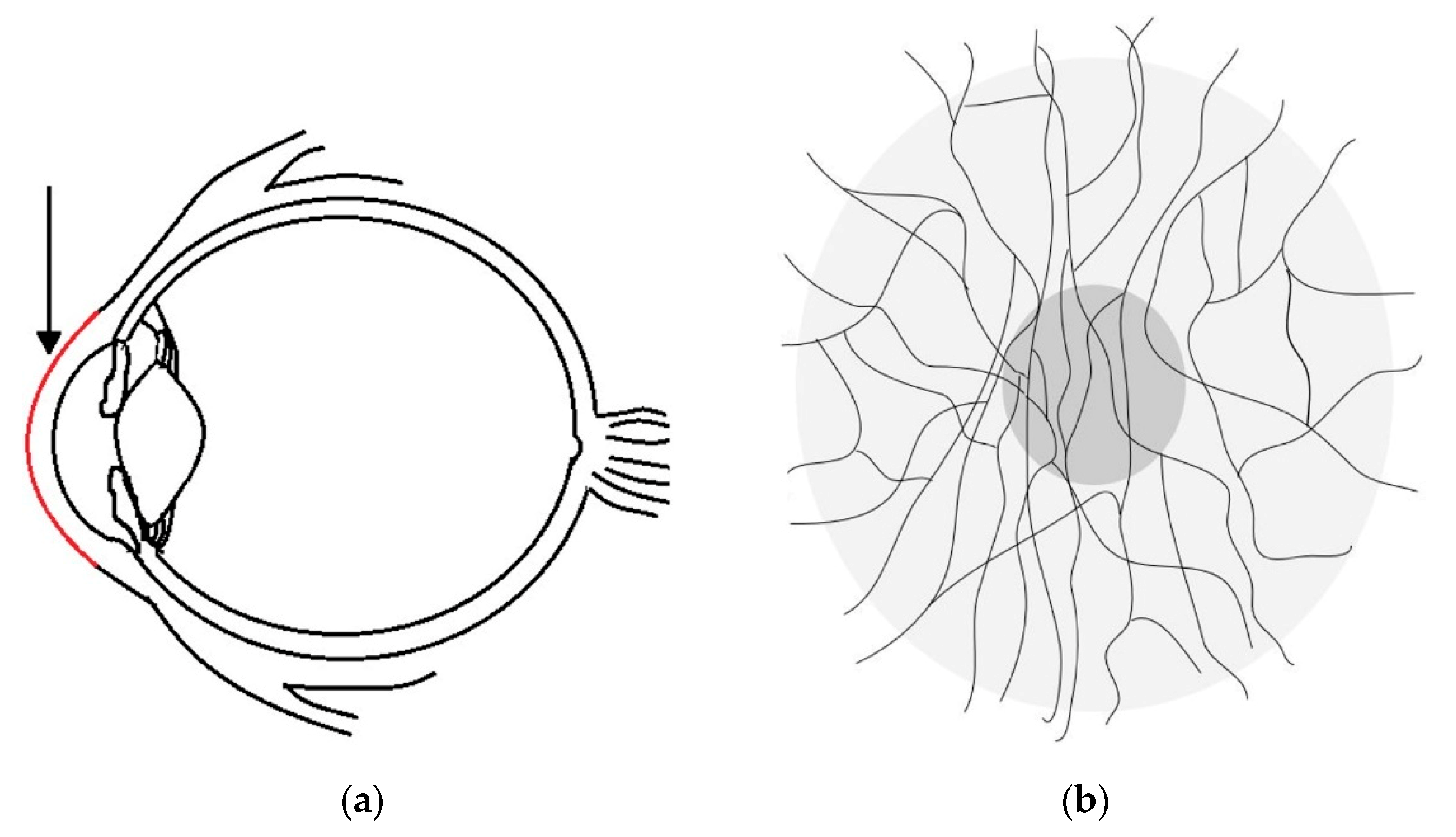
A major challenge for vision science is to estimate corneal nerve tortuosity from single images obtained by using in vivo confocal microscopy (IVCM) [1]. Eyes are composed of two fused pieces, both the posterior and anterior components [2]. The anterior component consists of the cornea, iris and lens. The cornea located at the front of human eyes is segmented into five layers [3]. Schlemm (1831) [4] discovered nerves between the two outermost corneal layers; their location is illustrated in Figure 2a,b (side view and front view). In the front view, the thin black lines show an approximate corneal nerve distribution of a healthy individual.
Eye diseases affect hundreds of millions of people worldwide [5]. Historically, a connection between diseases and nerve dysfunction was established in 1864 [6], but this research was not extended to corneal nerves until the late 20th century. In 2001, a breakthrough was achieved by Oliveria-Soto and Efron [7], when they successfully applied IVCM to corneal nerve imaging. Only three years later, in 2004, the first automated system analysing corneal nerves was described by Kallinikos [8]. Because corneal nerve tortuosity had been found to have a strong correlation with diabetic peripheral neuropathy and dry eye disease [9], it implied that corneal tortuosity analysis could be helpful for early eye disease diagnosis.
In the ongoing work, Scarpa et al., contributed several algorithms for corneal nerve tortuosity evaluation and provided publicly available corneal image datasets [10]. On the image acquisition side, Greenwald et al. [11] reviewed how confocal microscopy was used for imaging corneal structure. Additionally, as of 2015, confocal microscopy was the most popular imaging device next to optical coherence tomography (OCT) [12]. Among all the confocal microscopes, Tavakoli et al. [13] noted that “only the Nidek Confoscan 4 and Heidelberg Retina Tomograph HRT III combined with Rostock Cornea Module were commercially available” in 2012. In 2017, a new Rostock Cornea Module with a resolution of 1536 by 1536 pixels became available [14].
Despite the advances in image analysis, there has been no commonly agreed upon definition for corneal nerve tortuosity [15]. Lagali et al. [16] conducted experiments on expert graders with corneal nerve images. This investigation showed that a specific definition improves the agreement in tortuosity grading among experts. Specifically, the definition, “Grading only the most tortuous nerve in a given image,” results in the best intergrader repeatability [16]. Kim and Markoulli [15] compared different automated approaches for nerve analysis and produced tracing software to automatically segment contours in the corneal nerve and other medical applications.
Corneal nerve tortuosity could be graded into different levels linked to eye diseases [8] and was relevant for clinical diagnosis and prevention. Several tortuosity grading scales coexisted with a large number of highly different levels (Resolution from 3 to 800), as compared in Table 1. “Scale” represents the range of minimum to maximum “level,” and “interval” represents the increment (distance); i.e., for a scale from 1 to 10 there are 10 levels when only considering integers.
The most commonly used tortuosity grading method in the reviewed literature was manual grading; however, it was neither highly standardized nor free of problems. Manual grading was subjective, relied on the experience of the grader, and was difficult to compare and reproduce, as we show in the results section. It was therefore attractive to create a reliable automatic grading system for this measure.
1.1. Recent Work
Colonna et al. [20] suggested in 2018 to use U-Net convolutional neural networks for corneal nerve segmentation. They achieved segmentation sensitivity that in some instances exceeded human capability while maintaining acceptable runtime. Hosseinaee et al., also proposed a segmentation algorithm to trace sub-basal corneal nerves for in vivo UHR-OCT images [21] based on image contrast enhancement, thresholding and morphological operations.
In 2019, a study performed by Sturm et al. [22] revealed that image quality changed the quantification of corneal nerve parameters. In an experiment, images of 75 participants were assessed by semiautomated software and three subjects. They found that lower image quality caused lower tortuosity parameters. Wang et al. [23] created an architecture to evaluate optic nerve tortuosity using magnetic resonance imaging. They identified that optic nerve tortuosity may correlate with glaucoma. In summary, most reviewed recent publications focused on automatic cornea nerve segmentation but not on tortuosity estimations of the segmented nerves.
1.2. Purpose of This Work
The purpose of this study was to create a measure of tortuosity for normal healthy eyes that could then be used as a reference for future works on the diagnosis, detection and classification of eye diseases. We therefore sought to build automatic human corneal nerve tortuosity grading systems which may replace the time intensive and perceptually biased subjective tortuosity grading.
Our two primary research questions were: (i) How can we improve the corneal nerve tortuosity grading process? How are automated methods compared against subjective tortuosity gradings? and (ii) What is the ideal number of tortuosity grading levels?
2. Materials and Method
In this section we present one manual and three automated tortuosity grading methods. The manual method was used to establish a subjective grading baseline in Section 2.1. Each of the three automated methods presented in Section 2.2, Section 2.3 and Section 2.4 was then employed to predict our subjective grading baseline. Images were originally acquired from one eye of each of 24 individuals assessed to have normal, healthy vision. All images were de-identified for the purposes of this study. A minimum of 8 images were acquired from each eye from separate image regions with minimal overlap (less than 20%).
2.1. Subjective Grading Baseline
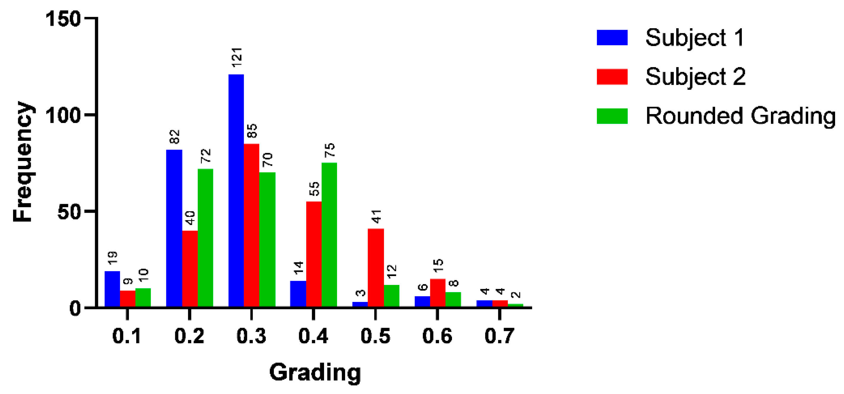
To establish a subjective grading baseline, we compared test subjects’ gradings of the same dataset with the 253 IVCM images. Each of the test subjects received IVCM images which were previously graded by an expert; then each subject graded other IVCM images on a scale of 0.1 to 1.0. The data were found to be imbalanced, with both subjects centring the data on class 0.3, as illustrated in Figure 3. This imbalanced distribution created challenges for our evaluation and machine learning models. Machine learning methods aim to minimize their training error; therefore, they are in turn “incentivized” to predict the dominant class, since it would be correct in more instances [24]. To mitigate this challenge, we created a balanced dataset based on gradings of two test subjects by averaging their ratings and rounding them down for gradings below 0.3 and up for gradings above 0.3. For example, 0.25 was rounded to 0.2 and 0.35 was rounded to 0.4. These data were labelled “rounded grading” in the Figure 3. We aimed to find the best balance of retaining the highest image quantity while having an equal number of images in each class.
2.2. Automated Tortuosity Estimation (Cfibre)
We implemented a custom modification for a freely available software package—Cfibre—which was originally developed by Kim and Markoulli [15] for automatically segmenting corneal nerves from IVCM images. The custom modification for our project was built on the standard functionality of Cfibre to add the automatic estimation of corneal nerve tortuosity from structural information on the segmented nerve contours. We intended to use this automated estimation of corneal nerve tortuosity as an objective approach for grading the tortuosity of corneal nerve images.
We assessed two previously proposed algorithms for tortuosity estimation before the implementation of our algorithm. The arc–chord ratio method was one of the simplest geometric methods for estimating the tortuosity of a curvilinear structure. It considered the length of the curve and divided it by the linear distance between its endpoints. This method had low computational requirements but did not consider many features of the nerves, such as different curvature amplitudes and changes in inflection points. Another assessed method was the absolute curvature method. It considered the integral of the curvature over the segment length to measure variable of the chord direction [10].
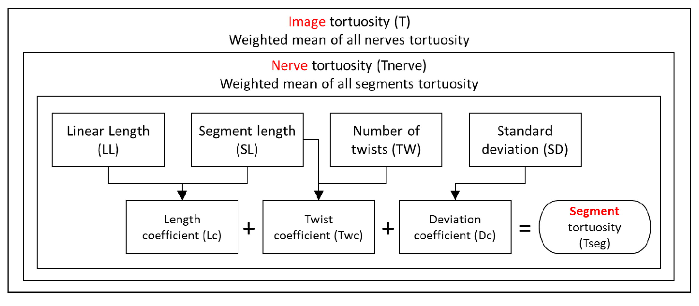
A single IVCM image provides only a small window to the structure of potentially far longer nerves in the neighbourhood of the sub-basal nerve plexus. We designed our objective analysis to separately estimate the tortuosity of every continuous nerve contour sampled by segmentation from each of the IVCM images. Pooling the results and weighting by length, we could achieve a global estimate of tortuosity for each image. This image tortuosity (T) was calculated from nerve tortuosity (Tnerve), which was calculated from segment tortuosity (Tseg). The entire Cfibre tortuosity grading process is shown in Figure 4:
To calculate segment tortuosity, we considered four key parameters for each segment: segment length (SL), linear length (LL), number of twists (changes in orientation) (TW) and standard deviation (SD). We then calculated three coefficients based on these parameters.
where Lc, Twc and Dc were the length coefficient, twist coefficient and deviation coefficient, respectively. The constant multiplicative value of 5 was found to generate objective results that were scaled to be consistent with the subjective grading scale. The tortuosity for each segment was then calculated as follows:
where Tseg was the segment tortuosity. This was repeated for all nerves. After the calculation of the tortuosity measure for each segment, the tortuosity of the nerve was calculated by taking the weighted average of all the segments as follows:
where Tnerve stands for Tortuosity nerve. The twist coefficient is calculated as follows:
where TW = sum of the twists of all segments and NL = sum of the length of all segments. Then a twist count was calculated as given below:
Twc = (TW/SL) if (TW/SL > 0.30) else 0
Dc = (SD/10) if (SD > 10) else 0
Tseg = Lc + (Twc × Dc) + (Dc/10)
Ntcnt = 1 if Ntwc > 0.40 else 0
This was repeated for all the nerves of the image. The tortuosity of the overall image was then calculated by taking the weighted average of all the segments and adding the nerve twist count:
where T was the image tortuosity.
Code Implementation in Cfibre
The baseline Cfibre version traced the nerves pixel by pixel (red channel used for marking nerve contours). The program checked if the pixels’ red channel was on, and if it was off, proceeded to the next pixel. If a colour value was found, it marked the first such pixel as white (i.e., all RGB channels on). It examined the eight surrounding pixels and repeated the above process. If two pixels were found with red colouration, it continued.
However, if more than 3 pixels were found, then it meant it was a junction point for the branches of the nerve. Junction pixels were then marked as yellow. If only one pixel with a red value was found, it meant that the pixel was the end point of the nerve. Such nerves were marked as white. This labelling was leveraged for our segmentation process. First, we created a new image wherein only the distinct points such as junctions and end points were marked; other points of the nerve were not marked. The baseline Cfibre version already used tracing code which calculated the nerve properties by traversing pixel by pixel along the points of the nerve. Subsequently, recursive calls were used to traverse along the nerve pixels. In this code, we were checking if a white or yellow point was found at each pixel location on the new image we created above. If the white pixel was found, we noted the coordinates. This was the starting point of the first segment of the nerve. As we traversed the nerve in the tracing code and found a yellow point at a pixel location in the new image, it meant that a junction was reached. We noted the coordinates of the yellow point. This point was marked as the end point of the segment. During the traversal of the nerve along the segment’s length, we were counting the number of twists as follows: For the first two pixels, we calculated the angle between those two pixels and stored it as the previous angle. From the third pixel onwards, we calculated the angle of the current pixel with the previous pixel. When this angle was the same as the previously stored angle value, then it meant that there was no change in orientation. If the angle was not the same, it meant that the orientation changed and we recorded the number of changes. The angle value then replaced the old value recorded for the previous angle. This process was repeated until the whole segment was traversed. For the angle calculation, we used the following mathematical expression which returns a scalar:
where, if (x1, y1) and (x2, y2) were the coordinates of the two pixels, then:
Angle = tan (x,y) × (180/pi)
x = |x1 − x2|
y = |y1 − y2|
Image tortuosity calculation was implemented following the process laid out in Section 2.2—calculating image tortuosity from nerve tortuosity, which was calculated from segment tortuosity. In detail, after a segment was identified in Cfibre, four of its properties were calculated: standard deviation, starting point, end point and number of twists. This process was iterated over the entire nerve until its end point was reached, while continuously writing all properties to a list.
Once the properties for all segments had been recorded, we iterated over the list of segments. For each segment, we calculated the linear length coefficient, twist coefficient and the deviation coefficient to calculate a segments tortuosity. Additionally, we recorded a segments length in a variable and the product of segment tortuosity and segment length in another variable.
After we iterated through all segments, we calculated the nerve tortuosity by taking the weighted mean using the variables mentioned above. We also calculated the nerve twist coefficient. If the value of this nerve twist coefficient was above a threshold (specifically 0.40 in our evaluation algorithm), we considered this nerve as more tortuous and added it in a variable. This process was repeated for all nerves. Once all nerves were accounted for, we calculated a weighted mean of all nerve tortuosities. We then added the count of more tortuous nerves to compute the overall image tortuosity. Finally, the output of the tortuosity of all the segments, nerves and overall tortuosity was displayed in the Cfibre console output. The analysis took approximately 12 seconds to complete for each image on a Surface Pro laptop.
2.3. From Segmentation to Automatic Tortuosity Estimation (USAAD)
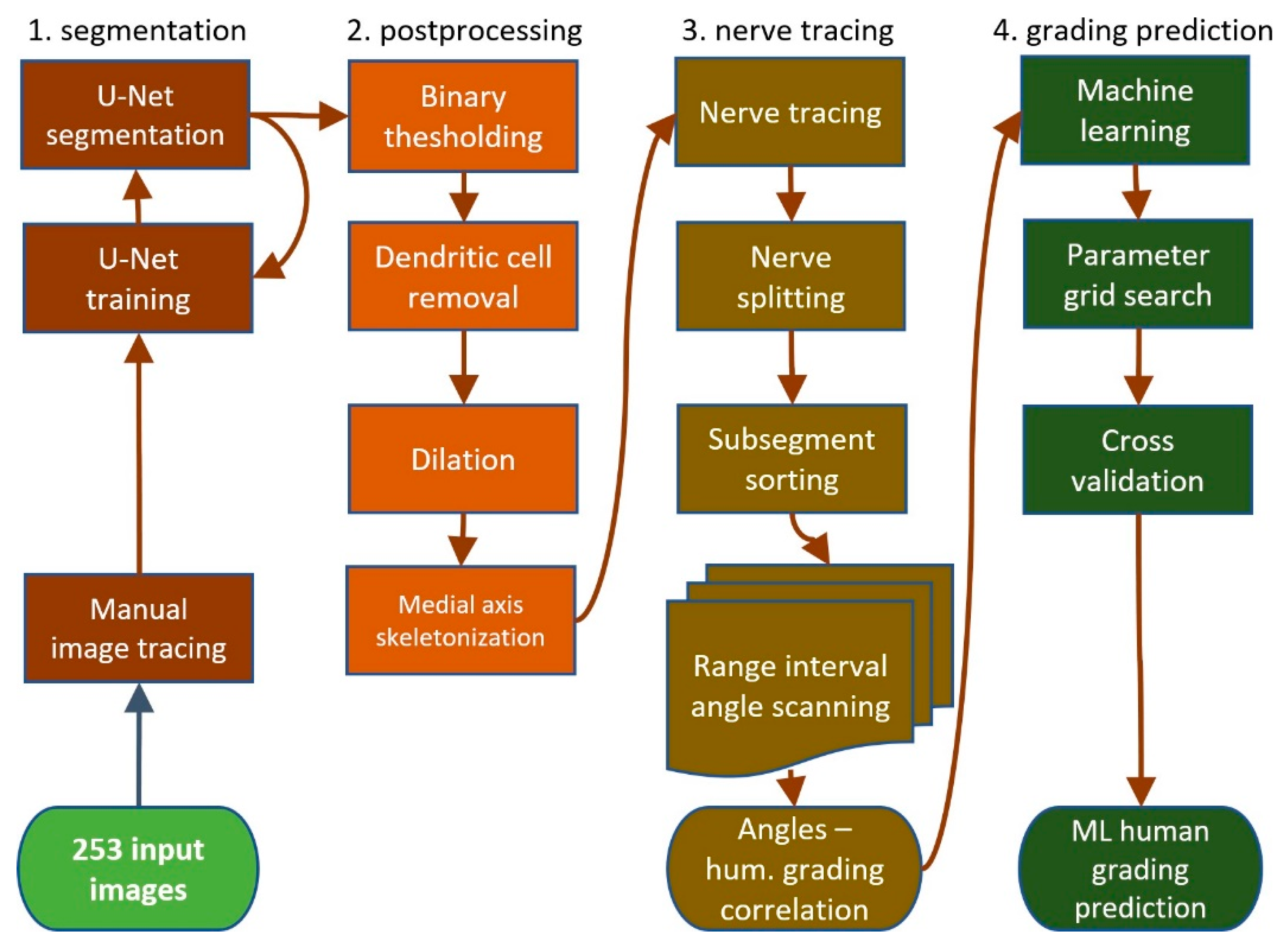
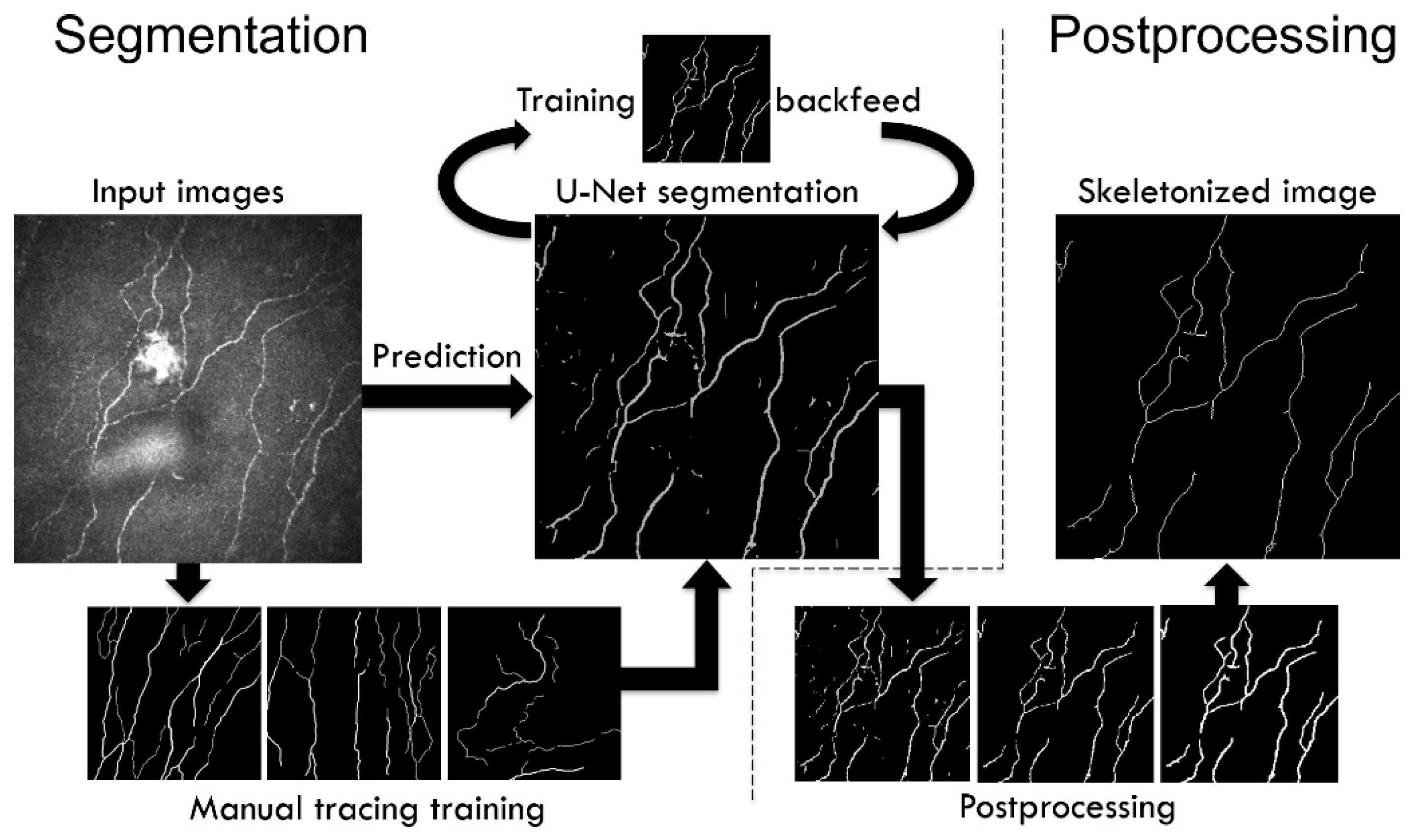
The U-Net segmented adjacent angle detection (USAAD) was a new multi-step approach, segmenting and tracing corneal nerves from images and then processing their properties. Subjective grading could then be predicted by comparing the properties of test images with those of training images, by machine learning, for example. This new approach was divided into the following steps: (1) Segmenting the IVCM images with a U-Net; (2) postprocessing to prepare the images for vectorization, (3) nerve tracing and property detection—the core of the new method; and (4) prediction of subjective grading based on nerve properties from (3), as shown in Figure 5.
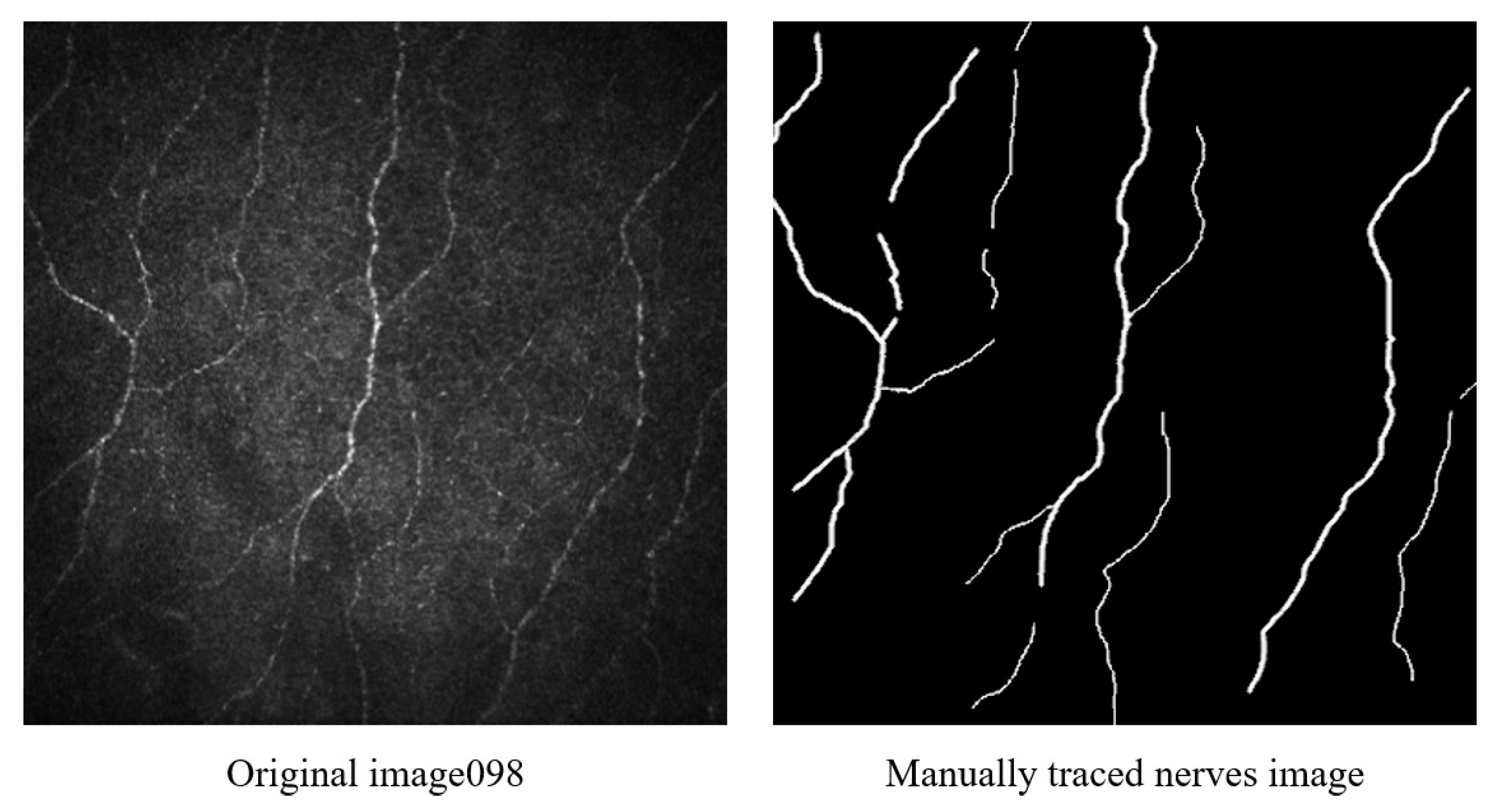
U-Nets are neural networks specialized in biomedical image segmentation [25]. They are based on convolutional networks and require only sparse training data consisting in our case of manually traced nerves. A small subset of the images with high spread was selected and the nerves manually traced using GIMP (GNU Image Manipulation Program) 2.10.8, as shown in Figure 6.
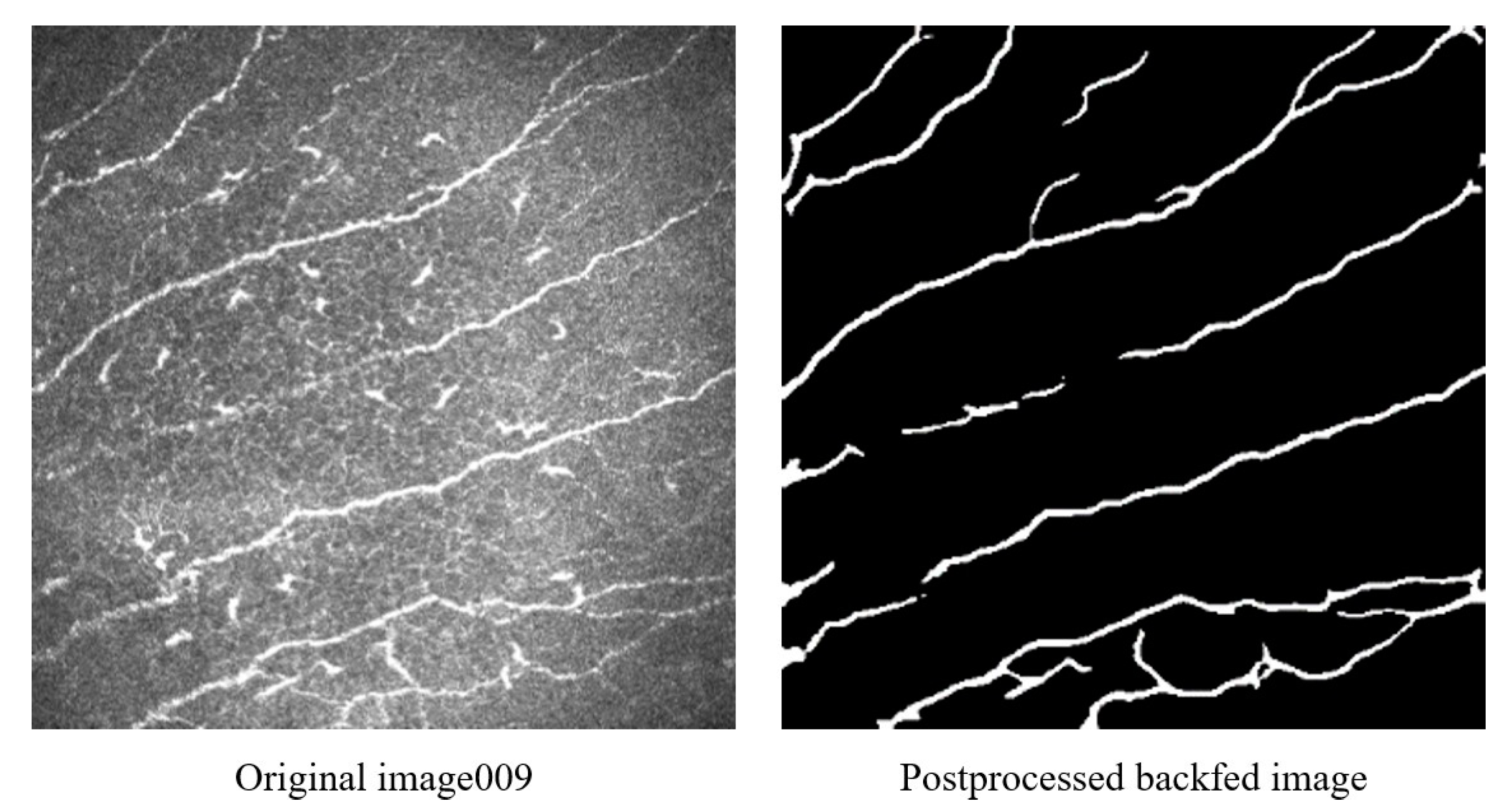
Since several U-Net implementations existed and we intended to focus on developing entirely new tortuosity grading methods, we chose to base our U-Net on a baseline version by Zhixuhao (2018) [26] to segment our images. As manual tracing of the images was a time intensive process and the impact of its quality was perceived to be high, additionally to manually tracing nerves, we devised a method to reuse the output of a selected number of images of the first generation of U-Net algorithms, as shown in Figure 7.
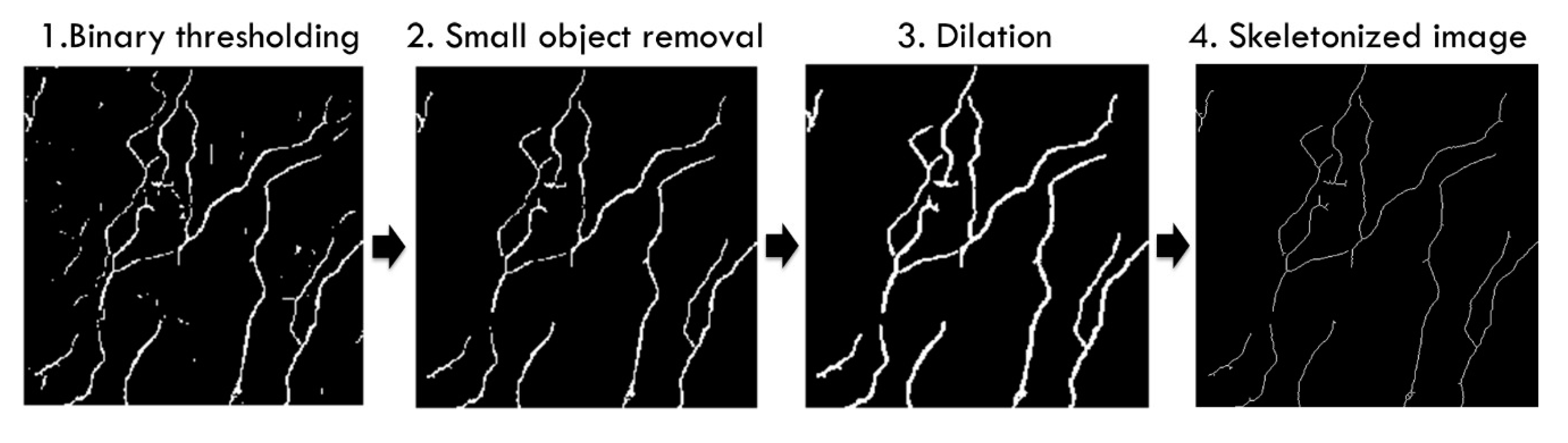
The segmented output from the U-Net was automatically post-processed to prepare the images for vectorization. To avoid false positives and backtracking, the desired inputs for the vectorization were images with no other whitened pixels other than the nerves reduced to thin lines. The postprocessing sequence, as illustrated in Figure 8, started by taking the output images of the U-Net, which were greyscale and not completely binary black or white.
The images were reduced to black or white using Otsu thresholding. The output images of the binary thresholding still showed remnant undesired noise and fragments; for example, dendritic cells visible as small white spots. Undesired fragments were automatically removed in the second postprocessing step, the small object removal, which was followed by dilation, a morphologic operation to broaden the nerves and fill small gaps. This uniform and wider nerve was then thinned to a line in the last step. Skeletonization was another morphologic operation which found the centreline of the nerves and reduced them to thin lines. The complete segmentation and processing sequence is shown in detail using images from the dataset in Figure 9.
The digital images in our dataset were rasterized. Such rasterized images had a dot matrix data structure and were composed of individual points called pixels; in case of our dataset, 384 × 384. We had to solve the same challenges as for the Cfibre approach, since we could not directly perform operations on the skeletonized raster images, such as finding nerve intersections or nerve endings. To perform these operations, all images were first converted into graphs. Our skeletonized images could be considered a square matrix with all individual points represented by 0 for black or 255 for white. The rasterized image data structure did not contain directly accessible information on which white pixels belonged to which nerves. We therefore converted all rasterized images into graphs to extract the numbers of nerves with their respective segments and all points on each segment. This was achieved by finding a first white pixel in the rasterized image by trying all x-positions at the y-position centreline of the image. If no white pixel was found, the y-position was moved in steps of:
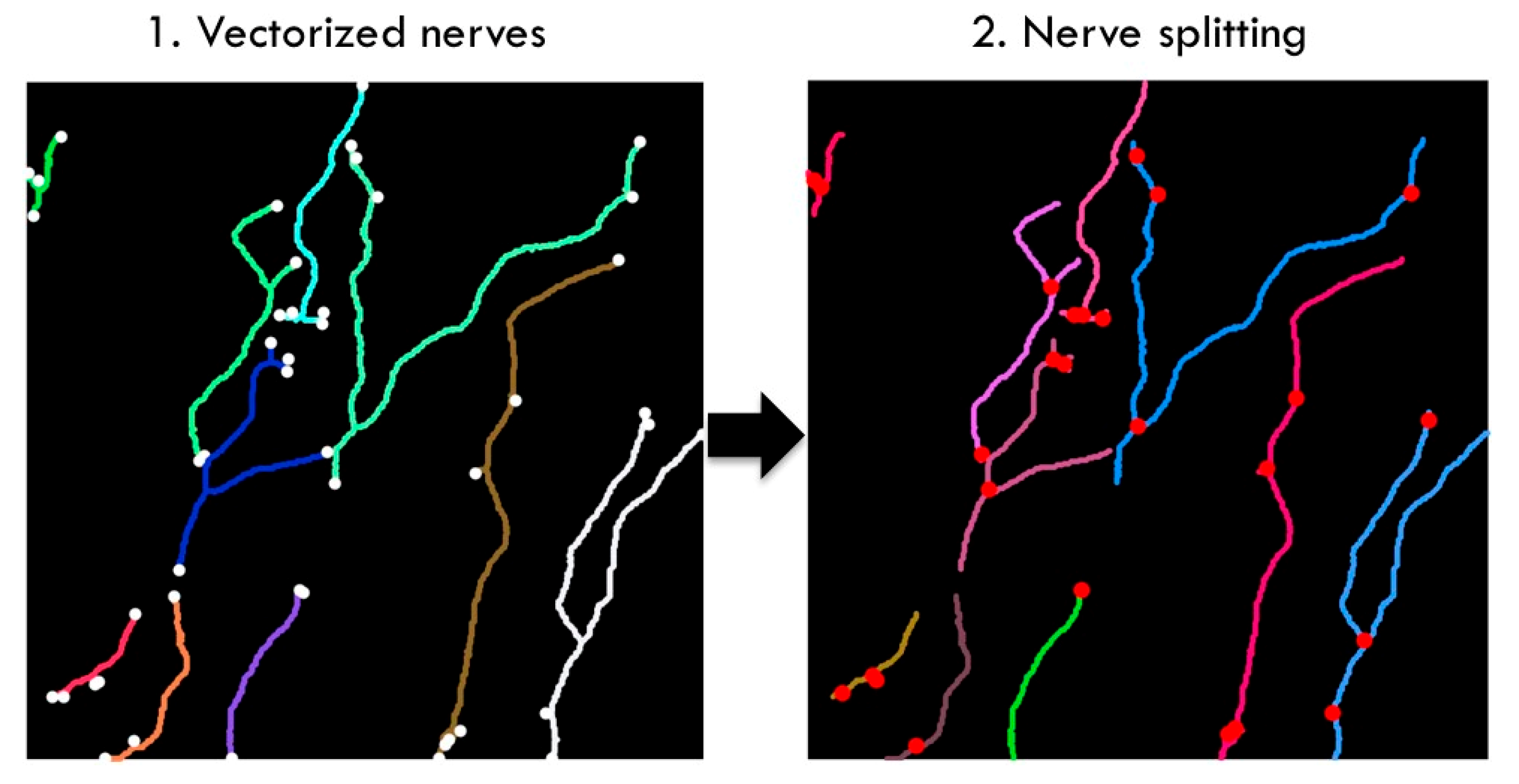
vertically until a white pixel was found. The algorithm then searched for a neighbouring white pixel and marked all that were scanned. It then centred itself on the next white pixel and repeated the search, until all white pixels of the nerve had been exhausted. All of the pixels that were found were then connected to a graph. As a next step, the algorithm searched for another white pixel by excluding the areas which had been marked as searched. To perform tortuosity calculations, we broke up the nerves into individual segments (Figure 10) at their intersections. Nerve branches tend to run in very different directions at these intersecting points, which could have caused our algorithm to consider intersections as indicative of high tortuosity.
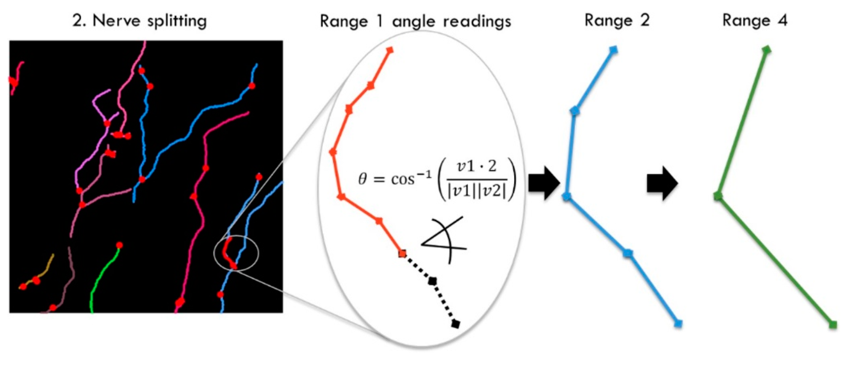
The nerve angle detection was a new key step of the adjacent angles’ detection method. To extract as much information from every nerve as possible, the angles between all vectors of each segment were measured in longer and longer intervals (Figure 11), referred to as ranges. This was achieved by calculating the direction of two adjacent vectors and calculating the angle θ:
This process was repeated from short to long ranges and for all nerve segments of all images until all angle readings were written to a dataframe. To check how well the results correlated, we calculated the mean of all the angles in each image and plotted it against the subjective grading for the respective image. The mean angle for one image was calculated as follows:
Our hypothesis was that averaging all angles leads to smoothing of the result and that human perception may have not been linear. For example, for a long nerve with one bend in the middle, the bend in the otherwise straight line would have stood out more to subjective grading. We therefore experimented with giving weights to each individual angle before calculating the average. We tested exponential, quadratic and cubic weights and achieved improved results for quadratic and cubic weights, with quadratic achieving the highest correlation.
The weights were intended to match subjective grading better; but we could not positively exclude that completely linear readings would potentially come closer to the desired analysis for medical applications. The mean adjacent angles could already be considered a tortuosity grading. In our next step, we optionally used the mean weighted adjacent angles to predict subjective gradings. This was achieved by taking the weighted angles for each range and averaging them, as explained in the previous section. The mean weighted angles for each range were used as to train machine learning methods. We recorded adjacent angles in from 1 to 80, but then discarded values below 12 and above 60, as explained in the Results section. For our final model, we considered 50 weighted angles as features for each image, from 12 to 60. Table 2 provides a statistic for two of these features, the weighted angles of 12 and 60. These were the shortest and longest ranges used to train our neural network.
Count was the number of all tested images. Mean, min, max and std refer to the mean, minimum, maximum and standard deviation of the number of weighted angles, and the values at (0.25–0.75) percentiles.
2.4. Direct Image Classifcation with Deep Learning
We have tested direct image classification performance of our balanced corneal nerve image dataset with AlexNet [27] and VGG-16 [28] implemented in Keras for a quantitative comparison with the previously introduced methods. AlexNet and VGG-16 are two convolutional neural networks developed for image classification. For both classifiers our balanced dataset was used with a train/test split ratio of 156/36 (81.25%/18.75%) and 6 classes. AlexNet and VGG-16 were trained on 26 images of each of the 6 classes and tested on 6 images of each class. For VGG-16 all images had to be resized from 384 × 384 to 128 × 128 to overcome memory limitations of the used GTX 970 GPU, while for AlexNet the native image resolution could be used.
3. Results
We compared four different tortuosity estimation methods: (i) a subjective grading baseline, (ii) an automated tortuosity estimation built on a previously published segmentation method, (iii) a completely new approach using segmentation and automatic tortuosity estimation and (iv) direct image classification using deep learning. We established a baseline accuracy for subjective corneal nerve tortuosity gradings. This baseline was created by re-grading the 253 IVCM images with two test subjects. Additionally, another informal experiment was conducted in which 10 experts were employed to grade the same four images. Two test subjects were asked to re-grade all 253 images on a scale from 0.1 to 1.0 in 10 steps. Both test subjects gave 70/253 (28%) images the same grading. Subject one graded the images on average 0.27 and subject two 0.36, respectively. The standard deviation between both gradings was 0.15 grades. Both subjects graded most images 0.3, but subject one graded 0.2 second most, and subject two graded images 0.4 second most, in line with subject two’s higher average gradings.
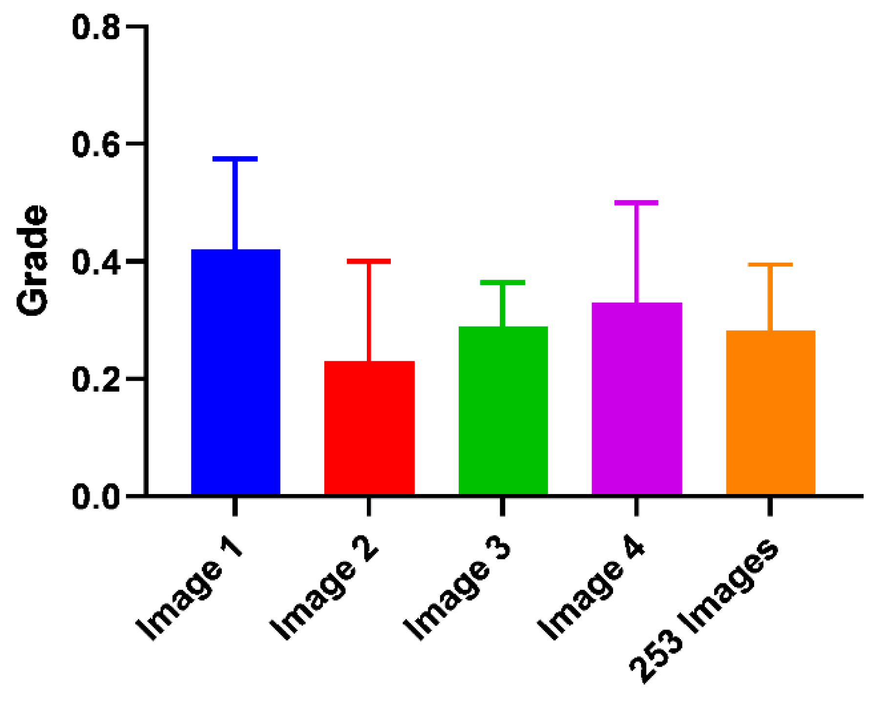
For the informal experiment, 10 experts in the clinical optometry domain were asked to grade four corneal nerve images (Figure 12). Image four was the same as image one but had three outliers going against the dominant direction of the other nerves removed. The average grade for image one was 0.42, and for image four 0.33, there was a difference of 0.09. The standard deviation for images one to four from the subjective grading bias experiment was plotted below as well as the manual grading comparison between two test subjects:
The difference in the average grade of images one and four was 0.09 compared to the standard deviation of 0.15 and 0.17 for these classes.
The Cfibre tracing performance percentage varied from 35% to 110%. In general, Cfibre had an average positive tracing rate of approximately 80%. The images with uniform illumination and high nerve-background contrast showed a high positive tracing rate of 75%–80%. For images with high variation in illuminance and low contrast, it achieved a lower tracing rate of around 40%. Some images showed percentages greater than 100%; this was due to false tracing of noise as nerves. For example, for images containing dendritic cells, the positive tracing was about 85%; however, this included false positive tracing of dendritic cells as nerves. Similarly, for some images the tracing percentage exceeded 100% due to false tracing. About 80% of all images in our dataset had a tracing rate ranging between 70% and 100%. For 18% of all images the tracing percentage was below 70%, while for 6 images the tracing percentage was over 110%.
In some images, branches were traced but not completely and they were not connected to their respective parent nerves. Thus, they seemed to appear as two separate nerves rather than one single nerve with multiple branches. Cfibre recorded the highest accuracy compared to subjective grading for class 0.1 with an accuracy of approximately 53%. Thus, it meant that the Cfibre approach could calculate the tortuosity for low tortuosity nerves but had a low accuracy for high tortuosity. The skewed distribution could be explained by four potential image-based causes: over-segmentation, incorrect thresholding, lack of precise definition of tortuosity and human perception in manual grading. Rather than only relying on accuracy, we evaluated the results on three more relevant metrics; namely, precision, recall and f1-score (Table 3). Precision was the ratio of correctly predicted images of all identified images of that class, and was around 0.34 for class 0.4 and 0.5–0.52 for class 0.6. Recall that the ratio of correctly predicted images to all images was between 0.34 for grades 0.3–0.5 and 0.56 for grade 0.1. Support was the number of samples in the respective class.
The first major intermediate result of the U-Net segmented adjacent angle detection method was the segmentation output of the U-Net and postprocessing. We assessed our segmentation performance by estimating the positive nerve tracing rate compared to manual nerve tracing for 20 random samples of our dataset. We particularly assessed segmentation performance regarding images with noise and anomalies. Some of these anomalies contained in IVCM images are buckling effects (Figure 1 C3). These are caused by curvatures in the corneal surface due to applanation of the imaging device. From 20 random samples out of our dataset, we subjectively estimated the positive nerve tracing rate compared to manual tracing as better than 80% despite buckling effects. The lowest positive tracing performance compared to manual nerve tracing was observed for images with low contrast (lower than Figure 6 left), which we estimated at ca. 60%. Although the true positive tracing performance was estimated to exceed 90% for images with many dendritic cells (Figure 7 left), dendritic cells also led to an increase in false positive tracing rate.
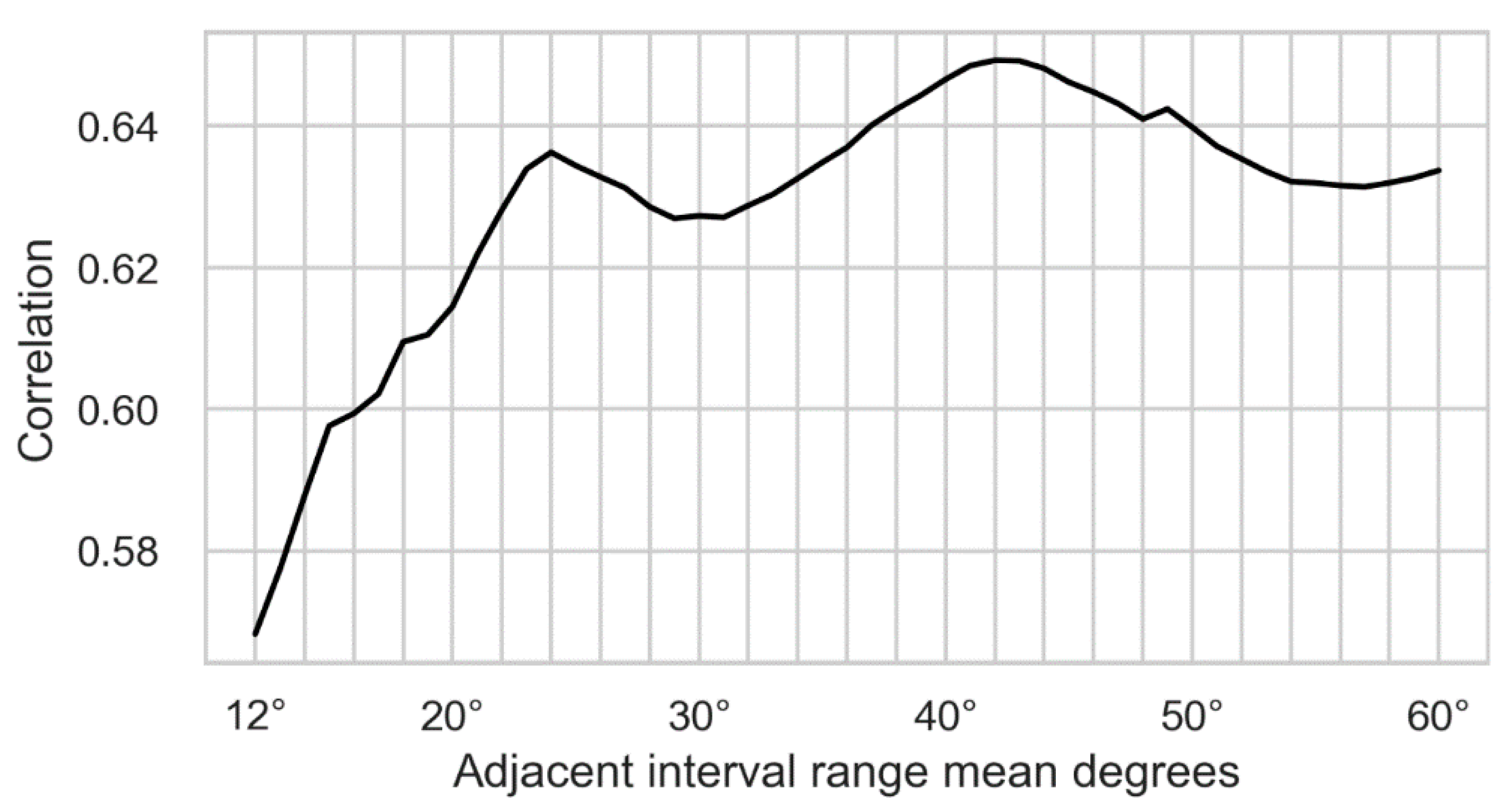
Initially, we recorded adjacent angles in a larger range, from 1–80, but then discarded ranges below 12 and above 60 for our dataset. Those ranges were removed for different reasons. For the prediction of subjective grading based on machine learning methods, it was required that the adjacent angles used for training showed a positive correlation with human grading. The adjacent angles were calculated for vectors on the raster given by the image pixels; therefore, the shorter the range, the fewer the possible discrete angles. This led to short ranges not exceeding a correlation significantly more than random chance, as can be observed by the correlation in Figure 13 dropping towards randomness on the left. The highest correlation of the weighted angles was achieved for range 44 at ca. 0.65.
Since adjacent angles were always calculated between two nerve segments, it was required to have at least two such segments in the image. The longer the range, the fewer segments a nerve could be broken down into. Specifically, an adjacent angle calculation of range of 60 required at least two nerve segments of at least 60 pixels in length each. For our dataset, the highest range of 60 was determined empirically and the number of suitable nerves dropped off steeply around this range. In Figure 13 the ranges are plotted on the x-axis and the correlation with human grading on the y-axis:
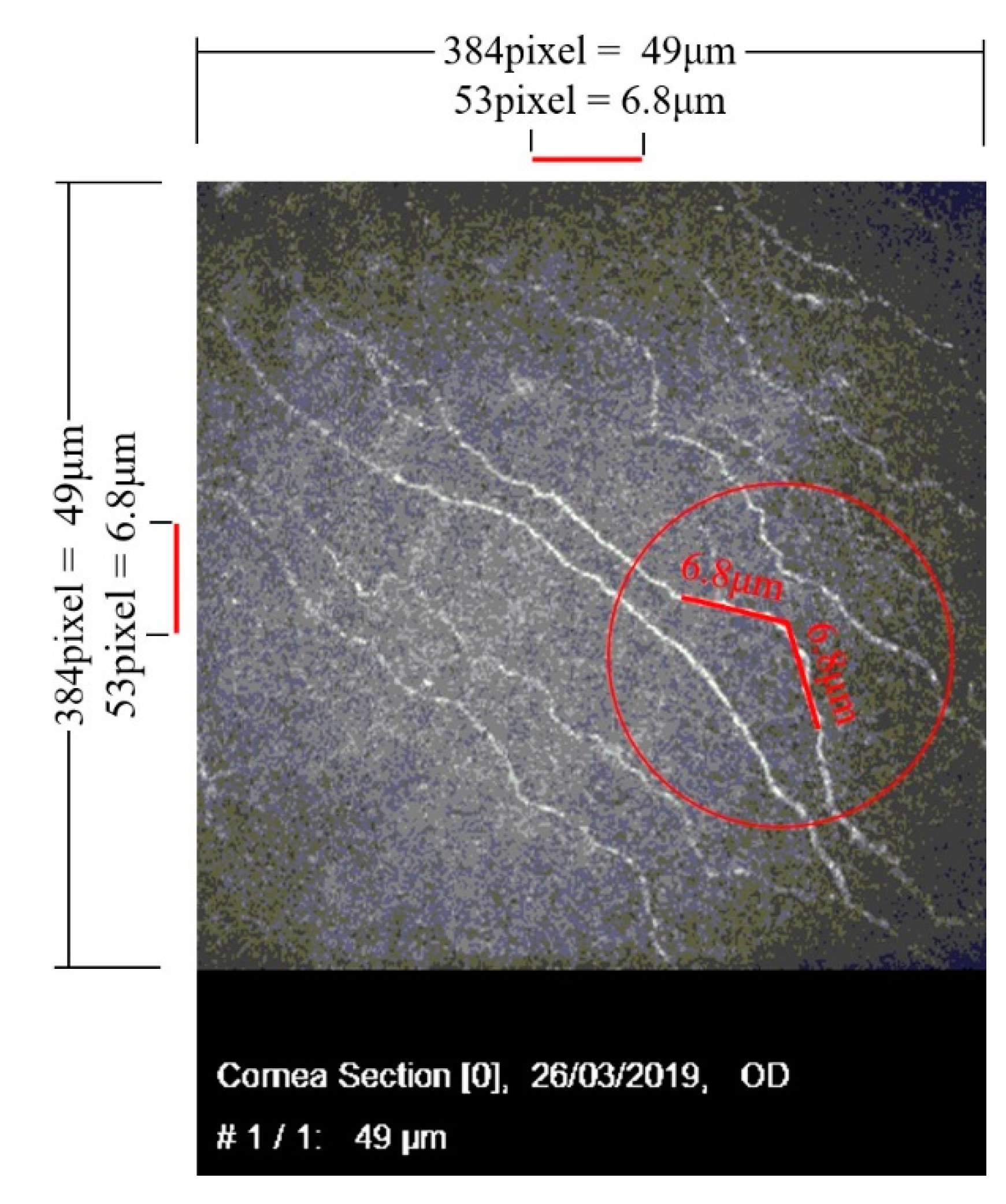
The number of vectors is dependent on the original image pixel grid, and therefore its resolution; they could also be converted into lengths. The microscope had a viewing area of 49 by 49 µm at a corresponding resolution of 384 by 384 pixels. To convert the vector range to µm, it had to be considered that a vector in parallel with the pixel grid had a smaller corresponding length than vectors of different orientation. The longest corresponding length resulted from vectors diagonal to the pixel grid with their equivalent length times √2 of those in parallel. A normal distribution of the nerve directions was assumed, and the length corrected on average between parallel and diagonal directions; this resulted in the following length correction factor:
With the correction factor Fncorrection, the nerve segment length that showed the maximum correlation with human grading could be calculated as follows:
Fncorrection × Maxcorrelatedrange = ≈ 53 pixel ≈ 6.8 µm
The maximum correlated range equivalent was plotted in Figure 14 to show the range in scale. Two highly correlated USAAD vector elements with an equivalent length of ≈6.8 µm are shown in the red circle.
Although the adjacent angles could be considered a corneal nerve tortuosity grading result, we also used the adjacent angles to predict a subjective grading using machine learning. The overall highest accuracy compared to subjective gradings of 41% was achieved with a multi-layer perceptron (MLP) classifier; its parameters were found by grid search. The parameters with the biggest effects were the hidden layer size and structure. The tolerance had to be increased to 0.0018 to ensure convergence. The overall accuracy could be increased to 43% by reducing the hidden layers to 1 × 120 instead of 2 × 60; however, this led to a very imbalanced prediction with accuracy of ca. 70% for class 0.1 and 0.6, but only random (20%) for class 0.3. The more balanced prediction of 2 × 60 layers was preferred and used in our final model. All results were 10x cross fold validated and the classification run 10× to average its results.
The overall accuracy (the ratio of correctly predicted images of all images) was 40%. Accuracy for the outermost classes 0.1 and 0.6 was highest, the prediction accuracy of all classes exceeded chance by at least 8%.
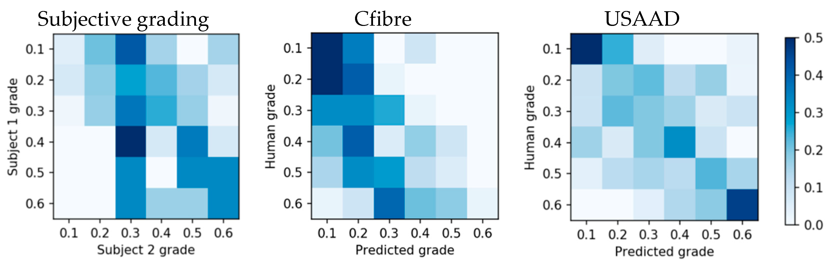
The subjective grading confusion matrix showed that the highest grading overlap was between grade 0.4 and 0.3 (Figure 15 left), instead of on the same grade, and its accuracy did not exceed chance for all grades. Compared to subjective gradings, Cfibre (Figure 14 center) showed high accuracy for images with low tortuosity, but lower accuracy with increasing tortuosity grade. No clear centreline is visible and accuracy did not exceed random for all grades. The centreline of the adjacent angle method (Figure 15 right) was most visible and the prediction accuracy exceeded random for all grades.
Direct image classification accuracy with AlexNet and VGG-16 did not yield results exceeding chance for our balanced dataset. AlexNet predicted a tortuosity of 0.1 or 0.5 for all images, depending on random seed initialization. VGG-16 permanently predicted a tortuosity of 0.6 for all test images. We compared how accurately Cfibre, USAAD, AlexNet and VGG-16 predicted the rounded tortuosity gradings of our two subjective graders. We used the average F1 score, a measure for test accuracy considering both precision and recall. Our dataset was balanced; therefore, the F1 average scores did not have to consider weights for each class. The results are shown in Table 4.
4. Discussion
Automatic curation of medical images has been in use in various domains of medical research [29,30]. In this research we show that automatic measurement of corneal nerve tortuosity is possible. We established a baseline for subjective corneal nerve tortuosity grading accuracy. For this task, two subjects received 13 images which were previously graded by an expert, two each of class 0.1–0.6. Only one image of class 0.7 was provided due to the limited availability of images in this grade. This was followed by each subject manually grading the 253 IVCM images on a scale of 0.1 to 1.0. Both test subjects’ gradings of our images were centred around class 0.3. The mean gradings were 0.27 and 0.36 respectively. The result showed both test subjects’ tortuosity grading maxima at 0.3. Randomly graded images collected of the eyes of the participants in this project supported this distribution; within 20 randomly graded images, none were more than 0.1 grades above or below 0.3. We measured a subjective grading normal deviation of 0.15 classes on a scale of 1.0 with 10 steps. This indicated that a subjective corneal nerve tortuosity grading scale of 10 steps was challenging, but not clearly an order of magnitude above what was possible.
For our informal experiment in which 10 experts each graded four images, we found that subjective gradings may have not been directly proportional to individual corneal nerve tortuosity. Our results indicated that outliers which strongly go against the otherwise dominant direction of the nerves may have swung subjective grading towards more tortuous. The mean grade for the image with the outliers removed was 0.09 lower on average in support of our hypothesis. However, the standard deviation of the manual gradings of these images by the 10 experts was relatively large (0.15 and 0.17) and not statistically significant. The standard deviations for the two unrelated images 2 and 3 were 0.17 and 0.07 respectively. For all subjective gradings, the standard deviation had always been between 0.07 and 0.17 relative to a scale of 0.1 to 1.0. This finding confirms that although 10 steps might be difficult to achieve by subjective grading, it is not too far off.
As evident from the results of the tortuosity estimation by Cfibre, we found that tortuosity estimates were highly skewed in favour of the first three grades. The reasons for this were assumed to be the following:
- Over-segmentation because the nerves were broken into individual segments at the intersection points.
- Human perception: The very fact that tortuosity gradings by subjects were partly influenced by their perception induced a lot of subjectivity, resulting in variation in the grading of the same image by different subjects. The image which may have been classified as 0.6 by one subject may have been graded as 0.3 by another.
- There was no universally accepted scientific definition of tortuosity.
USAAD produced several results which could be interpreted as corneal nerve tortuosity gradings. The first result related to the raw angles in multiple ranges. Before the quadratic weight was added and before the angles were averaged, this was a raw and linear measurement of the angles of all the nerves in the images. However, as also mentioned in the Cfibre discussion, it was not defined at the time of writing which exact tortuosity parameters were required for eye disease detection and prevention. It was not possible to assess whether these results or subjective grading results may have done better in this regard.
Both Cfibre and USAAD predicted all images of the balanced dataset better than chance, ranging from slightly below 30% to over 50%, and therefore possibly even better than our two subjects. Corneal nerve tortuosity gradings were found to have several problems which should be addressed in future. The biggest issue was that the desired morphological corneal nerve parameters for medical applications were not exactly defined. The most commonly used method was a subjective assessment which appeared to include a high statistical error and systematic error in some cases.
Direct image classification with AlexNet and VGG-16 did not exceed random accuracy for our dataset. We expected that this was caused by at least two reasons. Deep learning accuracy typically increases with training sample quantity, and a minimum number of training samples is required to exceed random accuracy. Cho et al., analysed prediction accuracy dependence on training sample quantity by training a convolutional neural network on medical datasets [31]. They used six classes of computed tomography images to train a GoogLeNet and systematically increased training dataset size, starting at five images per class. They exceeded random classification accuracy at 50 images per class.
We suspected that the second reason for not exceeding random accuracy with direct image classification was the similarity of the images in our dataset. Although we did not confirm this mathematically by, for example, calculating the Eucledian distance for the dataset by Cho et al., and ours, images in their dataset appear subjectively more dissimilar than ours; for example, a head CT image compared to a shoulder CT image.
The advantages of the proposed Cfibre and USAAD methods were that they were able to predict subjective grading with an accuracy better than chance for all classes. They outperformed direct image classification with AlexNet and VGG-16 for our dataset. Additionally, USAAD extracted raw tortuosity information from all nerves in a given image. These extracted short to long range angles were available for every nerve, which could be used for further medical analysis and development of a standardized corneal nerve tortuosity definition. We showed that these angles can be used to automatically predict subjective grading using machine learning.
We also identified disadvantages. Due to the limited availability of corneal nerve images, we could not show that our methods outperformed direct image classification for large datasets. The subjective tortuosity grading differed between two subjects; therefore, we suggest discussing and refining a standardized medical definition of corneal nerve tortuosity, for which our extracted raw angle data could be used.
5. Conclusions
Previous studies in the field have used tortuosity grading ranges that have been very limited [19] or broad [8]. Can the human visual system accurately differentiate between 0–8 levels in 0.01 intervals [10] or even between 0–70 tortuosity coefficients in 0.01 intervals [8]? We found slight variability in the frequency distribution of tortuosity ratings between graders using whole number intervals in our ten-point scale (1–10). However, the modal response was still centred around a value of three between graders. This would suggest that our 10-point scale was sufficient for characterising the shape of the true distribution in tortuosity parameters of corneal nerves imaged. The variability in uniformity of these estimates between graders would suggest that decimal-level sampling was not necessary for characterising the subjective estimation of these distributions. Indeed, if we were to use a three-point scale, we can expect there would have been greater correspondence in the distributions of subjective rating between our graders.
In our study, we used as many as 10 levels to observe some slight disintegration between these ratings. Although this range might seem large because it could be beyond the sampling resolution of the average subjective grader, it does offer added utility for future research. We found that the distribution of scores ranged up to six for our sample of images from normal healthy individuals. Based on previous research [8], we would anticipate a 50% increase in the mean distribution of tortuosity coefficients in some clinical populations (e.g., controls versus those with severe diabetic neuropathy). The 10-level scale would offer the dynamic range to accommodate this increase above the baseline we report in the current study.
Our results indicated that human corneal nerves may have been centred and normally distributed around what we measured as grade 0.3, with very low and very high tortuosity grades being rare. Our automated methods, especially the adjacent angle method, created more reproducible results which may have already exceeded subjective gradings depending on which exact parameters are desired. We also developed an entirely new tortuosity grading method which can extract a lot of information from corneal nerve images or other biomedical images and may have exceeded the amount of extracted nerve information of previous methods, which we will analyse in future work. We established that a grading scale of 10 steps was likely on the upper end of subjective grading accuracy, but in the right order of magnitude. This range also appears to be close to ideal for the automated methods, as well as subjective grading with additional improvements.
Author Contributions
M.K. and J.K. conceived, designed and supervised the project. S.M.Z., S.K.P. and M.M. supervised and provided intellectual contributions. P.M. executed the project and wrote the initial draft of the paper. All authors have read and agreed to the published version of the manuscript.
Funding
No extra funding.
Acknowledgments
We would like to thank Jeremy Chiang for taking IVCM images of our eyes, Duyen Hoang for preparing the grading scale and Fabio Scarpa for sending us IVCM images. We also thank Kushal Awadhare, Jiarong Song and Sarah Zhang for being members of capstone project. JK was supported by an Australian Research Council (ARC) Future Fellowship (FT140100535) and the Sensory Processes Innovation Network (SPINet).
Conflicts of Interest
The authors declare no conflict of interest.
References
- Edwards, K.; Pritchard, N.; Vagenas, D.; Russell, A.; Malik, R.A.; Efron, N. Standardizing corneal nerve fibre length for nerve tortuosity increases its association with measures of diabetic neuropathy. Diabet. Med. 2014, 31, 1205–1209. [Google Scholar] [CrossRef] [PubMed]
- Willoughby, C.E.; Ponzin, D.; Ferrari, S.; Lobo, A.; Landau, K.; Omidi, Y. Anatomy and physiology of the human eye: Effects of mucopolysaccharidoses disease on structure and function—A review. Clin. Exp. Ophthalmol. 2010, 38, 2–11. [Google Scholar] [CrossRef]
- Al-Waisy, A.S.; Ipson, S.; Malik, R.A.; Brahma, A.; Chen, X.; Al-Fahdawi, S.; Qah Waji, R. A fully automatic nerve segmentation and morphometric parameter quantification system for early diagnosis of diabetic neuropathy in corneal images. Comput. Methods Programs Biomed. 2016, 135, 151–166. [Google Scholar]
- Arnold, F. Anatomische und Physiologische Untersuchungen über das Auge des Menschen; University Library Heidelberg; Heidelberg, Germany, 1832; p. 28. [Google Scholar] [CrossRef]
- Yau, J.W.; Rogers, S.L.; Kawasaki, R.; Lamoureux, E.L.; Kowalski, J.W.; Bek, T.; Chen, S.J.; Dekker, J.M.; Fletcher, A.; Grauslund, J.; et al. Global prevalence and major risk factors of diabetic retinopathy. Diabetes Care 2012, 35, 556–564. [Google Scholar] [CrossRef] [PubMed] [Green Version]
- Rayaz, A.; Malik Andrew, J.; Boulton, M. Diabetic neuropathy. Ann. Der Phys. 1998, 82, 909–929. [Google Scholar]
- Efron NOliveira-Soto, L. Morphology of corneal nerves using confocal microscopy. Cornea 2001, 20, 374–384. [Google Scholar] [CrossRef]
- Kallinikos, P.; Berhanu, M.; O’Donnell, C.; Boulton, A.J.; Efron, N.; Malik, R.A. Corneal nerve tortuosity in diabetic patients with neuropathy. Investig. Ophthalmol. Vis. Sci. 2004, 45, 418–422. [Google Scholar] [CrossRef] [Green Version]
- Viola, F.; Mapelli, C.; Ratiglia, R.; Villani, E.I.; Galimberti, D. The cornea in sjogren’s syndrome: An in vivo confocal study. Investig. Ophthalmol. Vis. Sci. 2007, 48, 2017–2022. [Google Scholar]
- Ohashi, Y.; Ruggeri, A.; Scarpa, F.; Zheng, X. Automatic evaluation of corneal nerve tortuosity in images from in vivo confocal microscopy. Investig. Ophthalmol. Vis. Sci. 2011, 52, 6404–6408. [Google Scholar]
- Jesse, M.; Vislisel Mark, A.; Greiner Miles, F.; Greenwald Brittni, A. Corneal Imaging: An Introduction. 2016. Available online: http://webeye.ophth.uiowa.edu/eyeforum/tutorials/Corneal-Imaging/Index.htm (accessed on 15 October 2019).
- Shaheen, B.S.; Bakir, M.; Jain, S. Corneal nerves in health and disease. Surv. Opthalmol. 2013, 59, 263–285. [Google Scholar] [CrossRef] [Green Version]
- Tavakoli, M.; Petropoulos, I.N.; Malik, R.A. Assessing corneal nerve structure and function indiabetic neuropathy. Clin. Exp. Optom. 2012, 95, 338–347. [Google Scholar] [CrossRef] [PubMed]
- Stachs, O.; Sperlich, K.; Bohn, S.; Stolz, H.; Guthoff, R. Rostock cornea module 2.0–A versatile extension for anterior segment imaging. In Proceedings of the 2017 European Association for Vision and Eye Research Conference, Toronto, ON, Canada, 7 September 2017. [Google Scholar] [CrossRef]
- Kim, J.; Markoulli, M. Automatic analysis of corneal nerves imaged using in vivo confocal microscopy. Optom. Aust. 2018, 101, 147–161. [Google Scholar]
- Lagali, N.; Poletti, E.; Patel, D.V.; McGhee, C.N.; Hamrah, P.; Kheirkhah, A.; Tavakoli, M.; Petropoulos, I.N.; Malik, R.A.; Utheim, T.P.; et al. Focused tortuosity definitions based on expert clinical assessment of corneal subbasal nerves. Investig. Opthalmol. Vis. Sci. 2015, 56, 5102–5109. [Google Scholar] [CrossRef] [PubMed]
- Hart, W.; Goldbaum, M.; Côté, B.; Kube, P.; Nelson, M. Measurement and classification of retinal vascular. Int. J. Med. Inform. 1999, 53, 239–252. [Google Scholar] [CrossRef]
- Aggarwal, S.; Hamrah, P.; Trucco, E.; Annunziata, R.; Kheirkhah, A. A fully automated tortuosity quantification system with application to corneal nerve fibres in confocal microscopy images. Med Image Anal. 2016, 32, 216–232. [Google Scholar]
- Ruggeri, A.; Guimaraes, P.; Wigdahl, J. Automatic estimation of corneal nerves focused tortuosities. In Proceedings of the 2016 38th IEEE Annual International Conference of the IEEE Engineering in Medicine and Biology Society (EMBC), Orlando, FL, USA, 16–20 August 2016. [Google Scholar]
- Colonna, A.; Scarpa, F.; Ruggeri, A. Segmentation of Corneal Nerves Using a U-Net-Based Convolutional Neural Network; Springer: Berlin/Heidelberg, Germany, 2018. [Google Scholar]
- Hosseinaee, Z.; Tan, B.; Kralj, O.; Han, L.; Wong, A.; Sorbara, L.; Bizheva, K. Fully automated corneal nerve segmentation algorithm for corneal nerves analysis from in-vivo uhr-oct images. Ophthalmic Technol. 2019, 10858, 1085823. [Google Scholar]
- Sturm, D.; Vollert, J.; Greiner, T.; Rice, A.S.; Kemp, H.; Treede, R.D.; Schuh-Hofer, S.; Nielsen, S.E.; Eitner, L.; Tegenthoff, M.; et al. Implementation of a quality index for improvement of quantification of corneal nerves in corneal confocal microcopy images: A multicenter study. Cornea 2019, 38, 921–926. [Google Scholar] [CrossRef]
- Wang, X.; Rumpel, H.; Baskaran, M.; Tun, T.A.; Strouthidis, N.; Perera, S.A.; Nongpiur, M.E.; Lim, W.E.; Aung, T.; Milea, D.; et al. Optic nerve tortuosity and globe proptosis in normal and glaucoma subjects. J. Glaucoma 2019, 28, 691–696. [Google Scholar] [CrossRef]
- Barlow, H.; Mao, S.; Khushi, M. Predicting High-Risk Prostate Cancer Using Machine Learning Methods. Data 2019, 4, 129. [Google Scholar] [CrossRef] [Green Version]
- Brox, T.; Ronneberger, O.; Fischer, P. U-net: Convolutional Networks for Biomedical Image Segmentation. 2015. Available online: https://arxiv.org/abs/1505.04597 (accessed on 17 October 2019).
- Zhixuhao 2018, Implementation of Deep Learning Framework-Unet, Using Keras, GitHub Repository. Available online: https://github.com/zhixuhao/unet (accessed on 17 October 2019).
- Krizhevsky, A.; Sutskever, I.; Hinton, G.E. ImageNet classification with deep convolutional neural networks. In Proceedings of the 25th International Conference on Neural Information Processing Systems, Lake Tahoe, NV, USA, 14 December 2012; Curran Associates Inc.: Lake Tahoe, NV, USA, 2012; Volume 1, pp. 1097–1105. [Google Scholar]
- Simonyan, K.; Zisserman, A. Very Deep Convolutional Networks for Large-Scale Image Recognition. arXiv 2014, arXiv:1409.1556. [Google Scholar]
- Khushi, M.; Dean, I.M.; Teber, E.T.; Chircop, M.; Arthur, J.W.; Flores-Rodriguez, N. Automated classification and characterization of the mitotic spindle following knockdown of a mitosis-related protein. BMC Bioinform. 2017, 18, 566. [Google Scholar] [CrossRef] [PubMed] [Green Version]
- Khushi, M.; Edwards, G.; de Marcos, D.A.; Carpenter, J.E.; Graham, J.D.; Clarke, C.L. Open source tools for management and archiving of digital microscopy data to allow integration with patient pathology and treatment information. Diagn Pathol. 2013, 8, 22. [Google Scholar] [CrossRef] [PubMed] [Green Version]
- Cho, J.; Lee, K.; Shin, E.; Choy, G.; Do, S. How much data is needed to train a medical image deep learning system to achieve necessary high accuracy. arXiv 2015, arXiv:1511.06348. [Google Scholar]
Figure 1.
Comparison of straight and curved corneal nerves. (A) Low tortuosity nerve. (B) High tortuosity nerves. (C) Examples of (1) washout, (2) buckling and (3) dendritic cells.
Figure 1.
Comparison of straight and curved corneal nerves. (A) Low tortuosity nerve. (B) High tortuosity nerves. (C) Examples of (1) washout, (2) buckling and (3) dendritic cells.

Figure 2.
Corneal nerve position in the human eye: Side view—the cornea is marked in red and with an arrow (a). Front view (b).
Figure 2.
Corneal nerve position in the human eye: Side view—the cornea is marked in red and with an arrow (a). Front view (b).

Figure 3.
Grading histogram of the 253 IVCM images.

Figure 4.
Cfibre tortuosity grading process.

Figure 5.
U-Net segmented adjacent angle detection flowchart.

Figure 6.
Manually traced nerves.

Figure 7.
Example of images backfed to training.

Figure 8.
Scheme of postprocessing sequence.

Figure 9.
The flowchart of segmentation and postprocessing.

Figure 10.
Nerve vectorization and splitting, segment end points marked in white and intersections in red.
Figure 10.
Nerve vectorization and splitting, segment end points marked in white and intersections in red.

Figure 11.
Nerve angle detection process.

Figure 12.
Subjective grading and standard deviation.

Figure 13.
USAAD mean angle correlation with human grading.

Figure 14.
USAAD maximum correlated nerve length.

Figure 15.
Subjective, Cfibre and USAAD grading confusion matrices.


Table 1.
Comparison of available tortuosity grades and levels.
| # | Scale | Number of Levels | Reference |
|---|---|---|---|
| 1 | 0.0–1.0 (0.0 = straight, 1.0 = curved) | 11 levels; 0.1 interval | 1999 Hart [17] |
| 2 | 0–4 (0 = almost straight, 4 = frequent changes) | 5 levels; 1 interval | 2001 Oliveria-S. and Efron [7] |
| 3 | Tortuosity coefficients: 0–70 | 7001 levels, 0.01 interval | 2004 Kallinikos et al. [8] |
| 4 | 0–8 | 801 levels, 0.01 interval | 2011 Scarpa et al. [10] |
| 5 | 1–4 | 4 levels; 1 interval | 2016 Annuziata et al. [18] |
| 6 | Low, Medium, High | 3 levels | 2016 Guimaraes et al. [19] |
| 7 | 0.1–1.0: 0.1 = straight nerves, 1.0 = tortuous nerves | 10 levels; 0.1 interval | This work |
Table 2.
Statistical information for 12 and 60 weighted angles.
| Count | Mean | Std | Min | 0.25 | 0.5 | 0.75 | Max | |
|---|---|---|---|---|---|---|---|---|
| Range 12 | 192 | 6.7 | 2.371 | 2.8 | 5.1 | 6.4 | 8.0 | 16.2 |
| Range 60 | 192 | 173.2 | 108.4 | 32.7 | 96.9 | 148.9 | 221.3 | 913.9 |
Table 3.
Results comparison.
| Grade | Precision | Recall | F1-score | Support | |||
|---|---|---|---|---|---|---|---|
| Cfibre | AAD | Cfibre | AAD | Cfibre | AAD | ||
| 0.1 | 0.29 | 0.44 | 0.56 | 0.53 | 0.38 | 0.49 | 32 |
| 0.2 | 0.22 | 0.5 | 0.44 | 0.52 | 0.29 | 0.47 | 32 |
| 0.3 | 0.26 | 0.37 | 0.34 | 0.28 | 0.27 | 0.35 | 32 |
| 0.4 | 0.29 | 0.34 | 0.34 | 0.19 | 0.23 | 0.34 | 32 |
| 0.5 | 0.18 | 0.34 | 0.34 | 0.06 | 0.09 | 0.34 | 32 |
| 0.6 | 1 | 0.55 | 0.5 | 0.03 | 0.06 | 0.52 | 32 |
Table 4.
Prediction accuracy average of rounded average grading for four automated methods.
| Method | Cfibre | USAAD | AlexNet | VGG-16 |
|---|---|---|---|---|
| F1 score average | 22% | 42% | 17% | 17% |
© 2020 by the authors. Licensee MDPI, Basel, Switzerland. This article is an open access article distributed under the terms and conditions of the Creative Commons Attribution (CC BY) license (http://creativecommons.org/licenses/by/4.0/).
Share and Cite
MDPI and ACS Style
Mehrgardt, P.; Zandavi, S.M.; Poon, S.K.; Kim, J.; Markoulli, M.; Khushi, M. U-Net Segmented Adjacent Angle Detection (USAAD) for Automatic Analysis of Corneal Nerve Structures. Data 2020, 5, 37. https://doi.org/10.3390/data5020037
AMA Style
Mehrgardt P, Zandavi SM, Poon SK, Kim J, Markoulli M, Khushi M. U-Net Segmented Adjacent Angle Detection (USAAD) for Automatic Analysis of Corneal Nerve Structures. Data. 2020; 5(2):37. https://doi.org/10.3390/data5020037
Chicago/Turabian StyleMehrgardt, Philip, Seid Miad Zandavi, Simon K. Poon, Juno Kim, Maria Markoulli, and Matloob Khushi. 2020. "U-Net Segmented Adjacent Angle Detection (USAAD) for Automatic Analysis of Corneal Nerve Structures" Data 5, no. 2: 37. https://doi.org/10.3390/data5020037