Development of the Non-Iterative Supervised Learning Predictor Based on the Ito Decomposition and SGTM Neural-Like Structure for Managing Medical Insurance Costs

Tkachenko, Roman; Izonin, Ivan; Vitynskyi, Pavlo; Lotoshynska, Nataliia; Pavlyuk, Olena

doi:10.3390/data3040046

Open AccessArticle

Development of the Non-Iterative Supervised Learning Predictor Based on the Ito Decomposition and SGTM Neural-Like Structure for Managing Medical Insurance Costs^†

¹

Department of Publishing Information Technologies, Lviv Polytechnic National University, 79000 Lviv, Ukraine

²

Department of Automated Control Systems, Lviv Polytechnic National University, 79000 Lviv, Ukraine

^*

Author to whom correspondence should be addressed.

^†

This paper is an extended version of the paper: Vitynskyi, P.; Tkachenko, R.; Izonin, I.; Kutucu, H. Hybridization of the SGTM Neural-like Structure through Inputs Polynomial Extension. In Proceedings of the 2018 IEEE Second International Conference on Data Stream Mining & Processing (DSMP), Lviv, Ukraine, 21–25 August 2018; Lviv Polytechnic Publishing House: Lviv, Ukraine, 2018; pp. 386–391.

Data 2018, 3(4), 46; https://doi.org/10.3390/data3040046

Submission received: 23 September 2018 / Revised: 24 October 2018 / Accepted: 29 October 2018 / Published: 31 October 2018

(This article belongs to the Special Issue Data Stream Mining and Processing)

Download

Browse Figures

Versions Notes

Abstract

:

The paper describes a new non-iterative linear supervised learning predictor. It is based on the use of Ito decomposition and the neural-like structure of the successive geometric transformations model (SGTM). Ito decomposition (Kolmogorov–Gabor polynomial) is used to extend the inputs of the SGTM neural-like structure. This provides high approximation properties for solving various tasks. The search for the coefficients of this polynomial is carried out using the fast, non-iterative training algorithm of the SGTM linear neural-like structure. The developed method provides high speed and increased generalization properties. The simulation of the developed method’s work for solving the medical insurance costs prediction task showed a significant increase in accuracy compared with existing methods (common SGTM neural-like structure, multilayer perceptron, Support Vector Machine, adaptive boosting, linear regression). Given the above, the developed method can be used to process large amounts of data from a variety of industries (medicine, materials science, economics, etc.) to improve the accuracy and speed of their processing.

Keywords:

healthcare; medical insurance; prediction task; neural-like structures; Ito decomposition; Successive Geometric Transformations Model; non-iterative training algorithm

1. Introduction

Health insurance is one of the main directions of modern healthcare system development [1,2]. The prediction of individual health insurance costs is one of the most important tasks in this direction. The application of commonly used regression methods [3] does not provide satisfactory results in solving this task. In the big data era, the problem is deepened by the need for accurate and quick operation of such methods [4,5].

The existence of a large number of data leads to the possibility of using artificial intelligence to solve this task. The use of computational intelligence will allow for the hidden dependencies in the data set to be taken into account [6]. In most cases, it can increase the accuracy of individual health insurance costs prediction.

Existing neural network tools [7,8] demonstrate a sufficient accuracy of their work. However, they do not always provide the satisfactory speed of training procedures. The use of multilayer perceptron [9] for processing large amounts of data necessitates the use of large volumes of memory. In addition, this tool does not always provide satisfactory generalization properties [10]. The main drawback of the RBF networks for solving this task is that they provide only a local approximation of the nonlinear response surface [10]. Moreover, this method is characterized by a “curse of dimension”, which imposes a number of restrictions on its use for the processing of large amounts of data [11]. In the works of [12,13], the backpropagation algorithm is used to implement the training procedure. The large numbers of the epochs of this algorithm, as well as a large amount of input data, cause large time delays during its use.

Deep learning methods are associated with large time delays for training, long-term debugging procedures, and the need to interpret the output signals of each hidden layer. They are designed primarily for image processing tasks [14].

The training procedures of the known machine learning algorithms are fast [15]; however, these methods are inferior to the accuracy of the prediction results [16].

That is why it is necessary to develop new or improve existing individual insurance costs prediction methods and tools that would provide high prediction accuracy with sufficient training speed.

2. Data Description

2.1. Data Analysis

To solve the regression task, the medical insurance cost prediction dataset (Dataset: https://www.kaggle.com/mirichoi0218/insurance. Dataset License: Open Database) was selected from Kaggle [17]. It contains 1338 observations of the personal medical insurance cost. Each vector includes six input attributes and one output (Table 1). The task is to predict individual costs for health insurance.

We will consider all independent variables in more detail:

Insurance contractor age (Age). The minimal age of the insurance contractor is 18 years, maximum is 64 years, and the average age of the entire sample is 39.2 years. Insurance contractor age included 574 young insurance contractors (18–35), 548 senior insurance contractors (35–55), and 216 elder insurance contractors (>55).
Body mass index (BMI). This is the ratio of the person’s height to their weight (kg/m²). Minimal BMI is 15.96, the maximum is 53.12, and the average is 30.66. It is higher than normal.
The number of dependents (Children). This is the number of children covered by medical insurance. This indicator ranges from 1 to 5, and the average is 1095.
Smoking (Smoker). The dataset contains 1064 smokers and 274 non-smokers.
Beneficiary’s residential area in the United States (Area). This column displays four regions of the United States, where the number of observations for each of them is northeast: 324, northwest: 325, southeast: 364, and southwest: 325.

The individual insurance costs (IIC) is an output variable.

2.2. Data Preparation

We will make a series of transformations of the input data in order to represent them from a text in a numerical form (binary system coding). In particular, we will add five new columns as follows: Each column of the Insurance contractor gender and Smoking will turn into two; namely, male (M) and female (F), and smoker and non-smoker, respectively. The column Beneficiary’s residential area in the United States will be transformed into four different ones, each of which will be located in one of the four U.S. regions: Area 1 is Southwest, Area 2 is Southeast, Area 3 is Northwest, and Area 4 is Northeast. Thus, a new data sample was obtained. The vectors of each of the 1338 observations contain 11 input numeric attributes. They are given in Table 2.

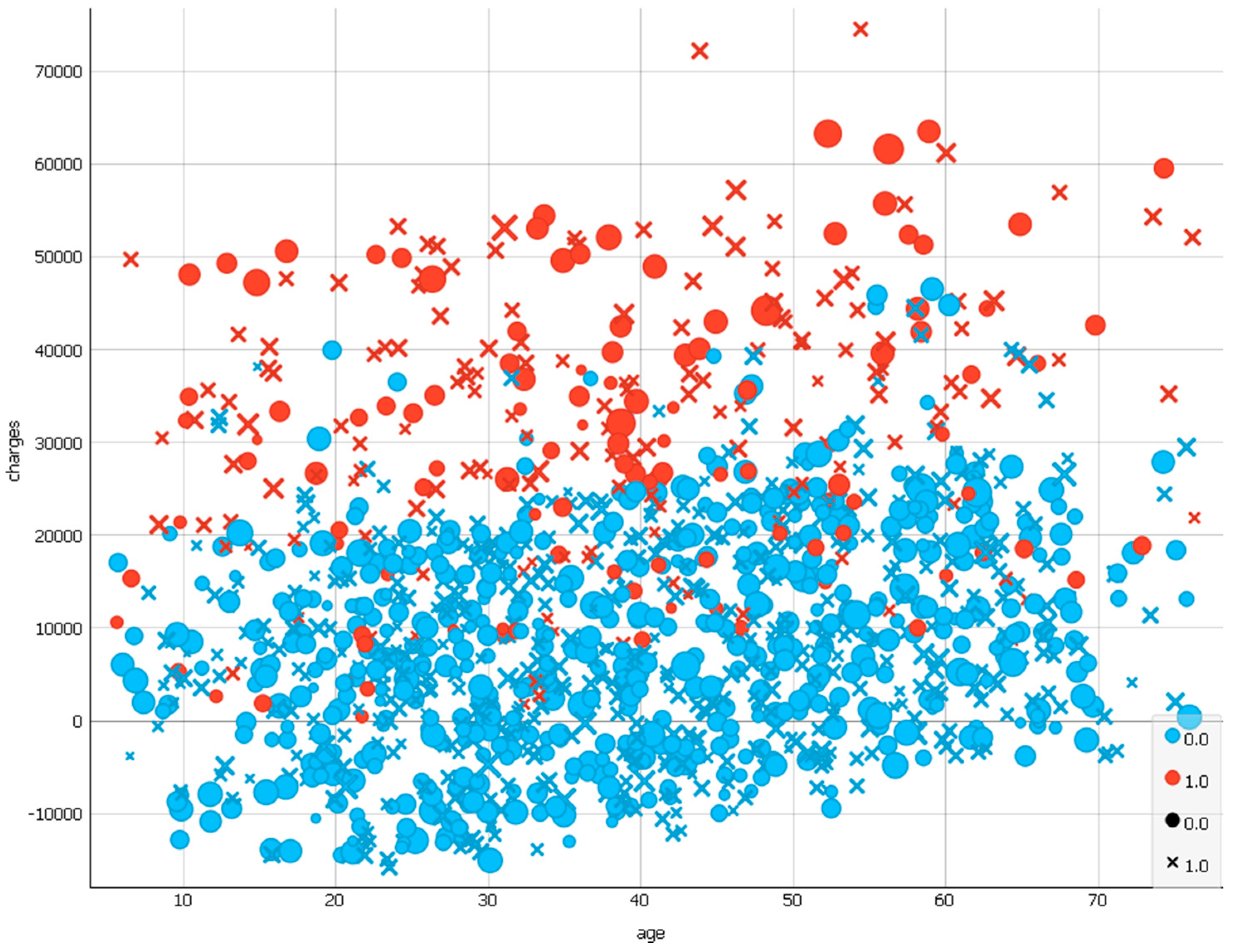
Figure 1 shows the scatter plot of the dataset from Table 2 using Orange Software, version 3.13.0. [18].

3. Predictor Based on the Ito Decomposition and Neural-Like Structure of the Successive Geometric Transformations Model (SGTM)

This paper proposes a new method focused on high-speed realization and universal application for regression and classification tasks.

3.1. Linear Neural-Like Structure of the Successive Geometric Transformations Model

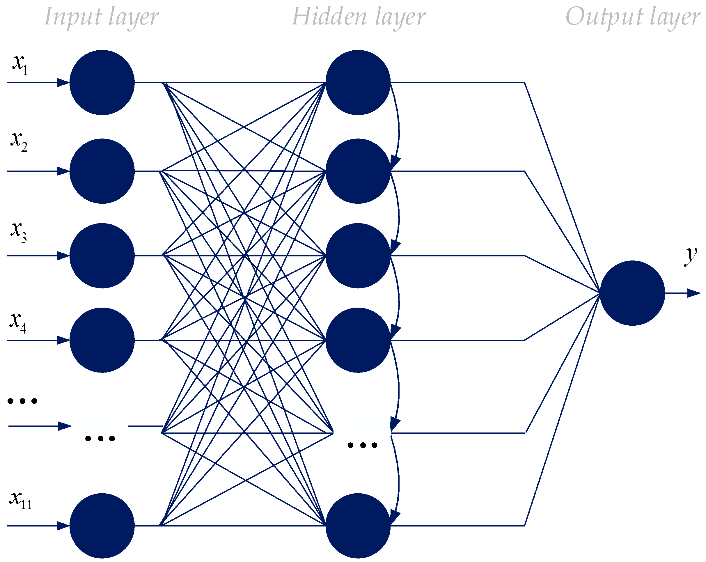
The authors of [19] have described the topology and the training algorithm of the new non-iterative neural-like structure for solving various tasks. It is based on the successive geometric transformations model (SGTM), and can work in supervised and unsupervised modes. The topology of this linear computational intelligence tool is demonstrated in Figure 2. Its feature is ordered as lateral connections between adjacent neurons of the hidden layer. The procedures of training and functioning of this instrument are of the same type.

The greedy non-iterative training algorithm ensures the repetition of the solution and allows using the common SGTM neural-like structure for processing large amounts of data effectively. Detailed mathematical descriptions and flowcharts of the training and operation procedures of the common SGTM neural-like structure are given in the work of [20].

3.2. The Ito Decomposition

The accuracy of the approximation task for nonlinear dependencies is one of the important tasks for processing large amounts of data. Existing machine learning methods do not always provide an opportunity for their use to obtain sufficiently precise results for solving this task.

According to the Weierstrass theorem, any continuous function in the given interval can be arbitrarily precisely described by a series of polynomials [21]. Another mathematical proof of the approximation of any continuous function is the universal approximation theorem (the expansion of the Weierstrass theorem).

The Ito decomposition (Kolmogorov–Gabor polynomial) is widely used for the development of various nonlinear approximation models [22,23,24,25,26]. The general view of the second degree polynomial can be written as follows [6]:

Y (x_{1}, \dots, x_{n}) = a_{i} + \sum_{i = 1}^{n} a_{i} x_{i} + \sum_{i = 1}^{n} \sum_{j = i}^{n} a_{i, j} x_{i} x_{j}

(1)

Under the conditions of processing of large amounts of multiparametric data, the searching of the polynomial’s coefficients is a non-trivial task. Existing methods, in particular, the least squares method and singular decomposition, do not provide sufficient speed [6]. That is why the application of the Kolmogorov–Gabor polynomial for the elaboration of the big data processing models requires the development of new, more efficient algorithms for the searching of its coefficients.

3.3. The Composition of the Non-Iterative Supervised Learning Predictor Using Ito Decomposition

The proposed linear non-iterative prediction method is based on combining the use of the Ito decomposition (Kolmogorov–Gabor polynomial) and SGTM neural-like structure [6]. Input (dependent) parameters according to the method are represented as members of this polynomial. The SGTM neural-like structure is used to find the Kolmogorov–Gabor polynomial’s coefficients. The benefits of such process are fast training, as well as the repetition of the solution. 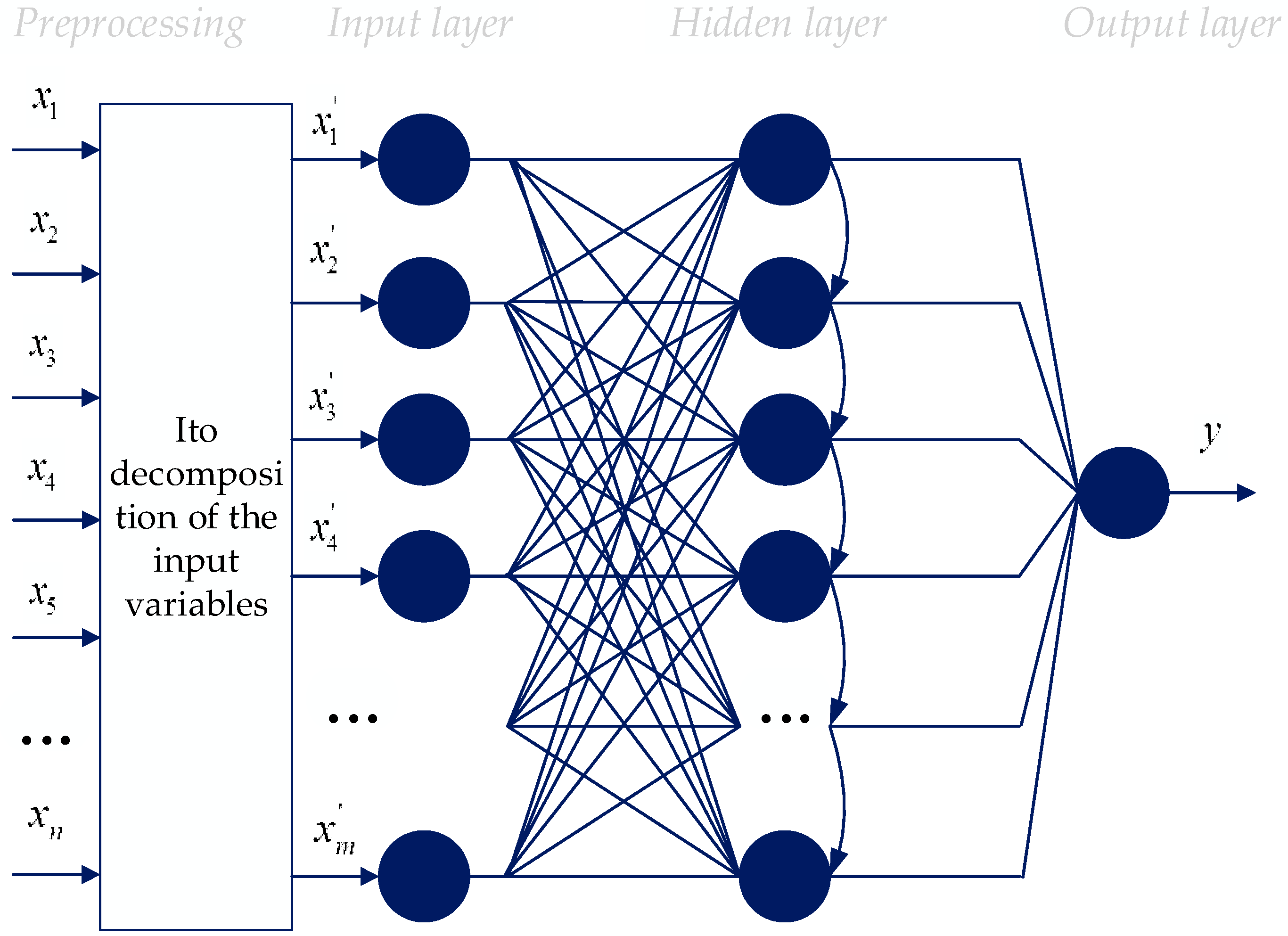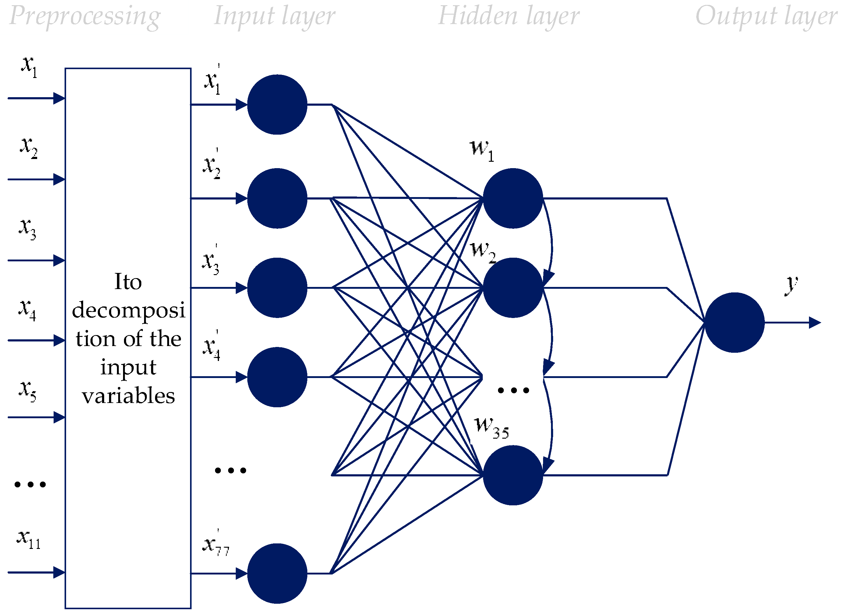Figure 3 demonstrates the topology of the proposed non-iterative neural-like predictor, which contains two blocks [6].

The input data is converted in the first block (preprocessing) (1). The number of input layer’s neurons of the proposed method when choosing a second-degree polynomial can be calculated according to the following formula [6]:

m = n + \frac{n (n + 1)}{2},

(2)

where

n

is the number of initial inputs from Table 1 (

n = 11

)

As the result of the fast, non-iterative training, the coefficients of the Kolmogorov–Gabor member are calculated in the hidden layer of the proposed model’s second block (Figure 3). Then, they are used to solve the task [6].

4. Modelling and Results

The simulation of the proposed method was carried out using the author’s software (console application). The main parameters of the computer on which the experiments were carried out are as follows: memory: 8 Gb Intel^® Core(TM) i5-6200U CPU, 2.40 GHz.

The parameters of the proposed method (SGTM + Ito decomposition) are as follows: 77 neurons in the input and hidden layers, 1 output. The second-degree Kolmogorov–Gabor polynomial was chosen for modeling. The mean absolute percentage error (MAPE) for the proposed method was 30.82%.

The mathematical basis for the direct dissemination networks application with the one hidden layer to the solution of approximation tasks is the universal approximation theorem. According to the theorem, the accuracy of the best approximation is obtained with a large number of neurons in the hidden layer [27]. However, in this case, according to the authors of [28], there is a possibility of overfitting.

A necessary estimation of the proposed method’s work is the indicator of the model’s complexity ratio to the accuracy of its work [24,29]. The complexity of the model, in this case, is influenced by two parameters; namely, the degree of the Kolmogorov–Gabor polynomial (which is why the second degree polynomial has been chosen) and the number of hidden layer’s neurons of the SGTM linear neural-like structure. The conducted experimental studies have demonstrated that the number of the polynomial’s coefficients, which are formed in a hidden layer, make a very small contribution to obtaining the exact result. However, their calculation greatly increases the duration of the method. That is why the research was conducted in order to determine the optimal complexity model for the proposed method. The results of this experiment are listed in Appendix A, Table A1.

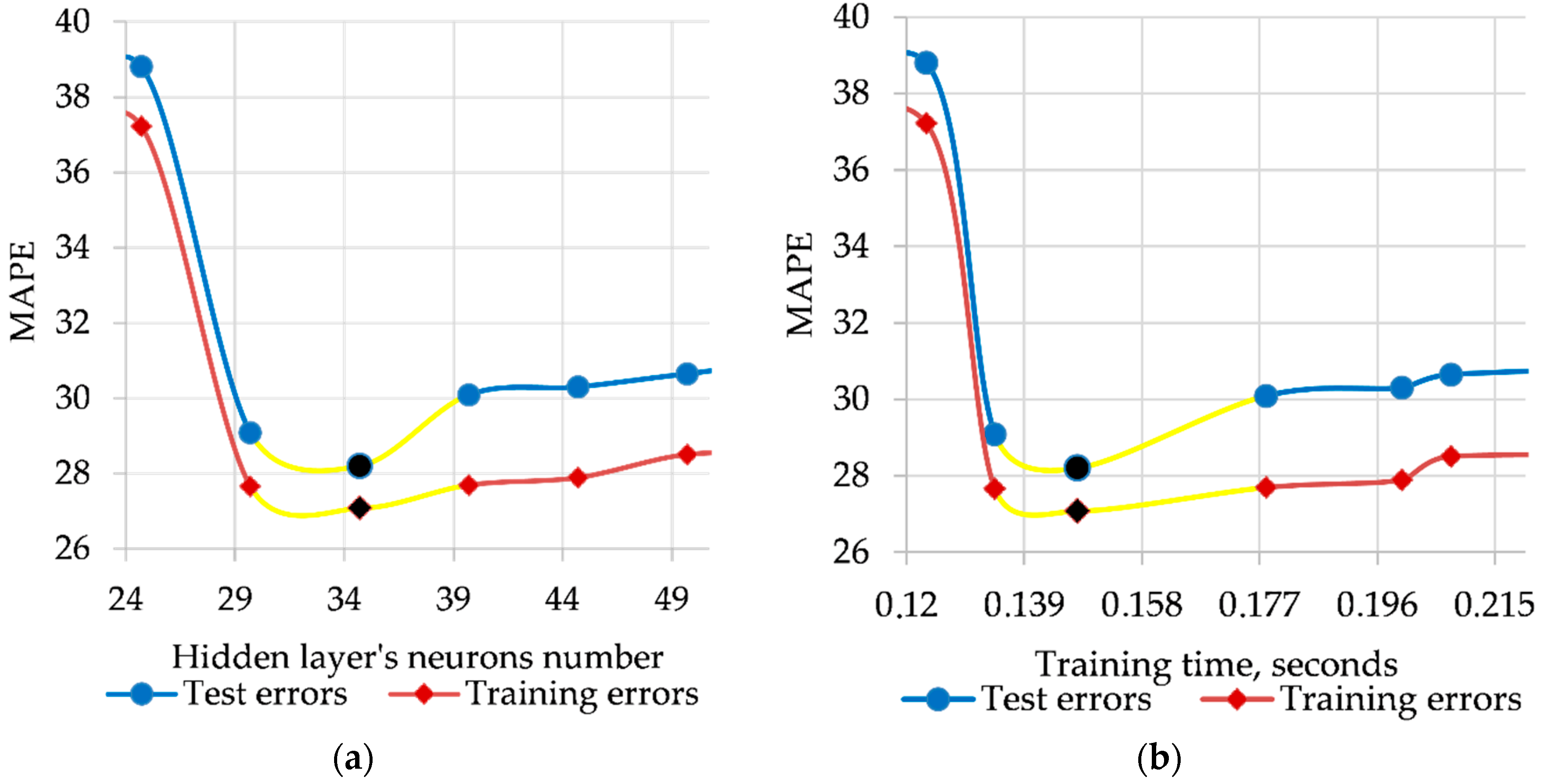
Figure 4a demonstrates the ratio of the neurons number in the hidden layer of the proposed method to the accuracy of the work (MAPE) on the interval 25–50 neurons with a step of 5. As can be seen from Figure 4, the optimal result of the method is 35 neurons in the hidden layer. All other indicators in Appendix A, Table A1 demonstrate the same result. Figure 4b confirms the obtained result regarding the duration of the training procedure.

The training procedure for the optimized version of the method is much shorter than training of the proposed method without optimal parameters selection. In addition, by reducing the number of neurons in the hidden layer from 77 to 35, it was possible to neutralize the effect of noise components. The topology of the optimized version of the method is demonstrated in Figure 5.

Table 3 provides quantitative indicators for evaluating the work of the developed method and its optimized version in terms of both training and testing modes according to the following indicators [30,31]:

Mean absolute percentage error (MAPE);
Sum square error (SSE);
Symmetric mean absolute percentage error (SMAPE);
Root mean square error (RMSE);
Mean absolute error (MAE).

As can be seen from the table, the optimal parameters selection of the proposed method (according to all five indicators) allowed the following:

to increase the generalization properties of the method (the difference between the MAPE indicators in the training and testing modes is 2.40% and 1.12%, respectively, for the developed and optimized methods);
to increase the accuracy of the optimized method by 1.34%.

In addition, it was possible to reduce the duration of the training procedure by 0.22 s. In terms of big data processing, all of the above are significant advantages.

5. Comparison and Discussion

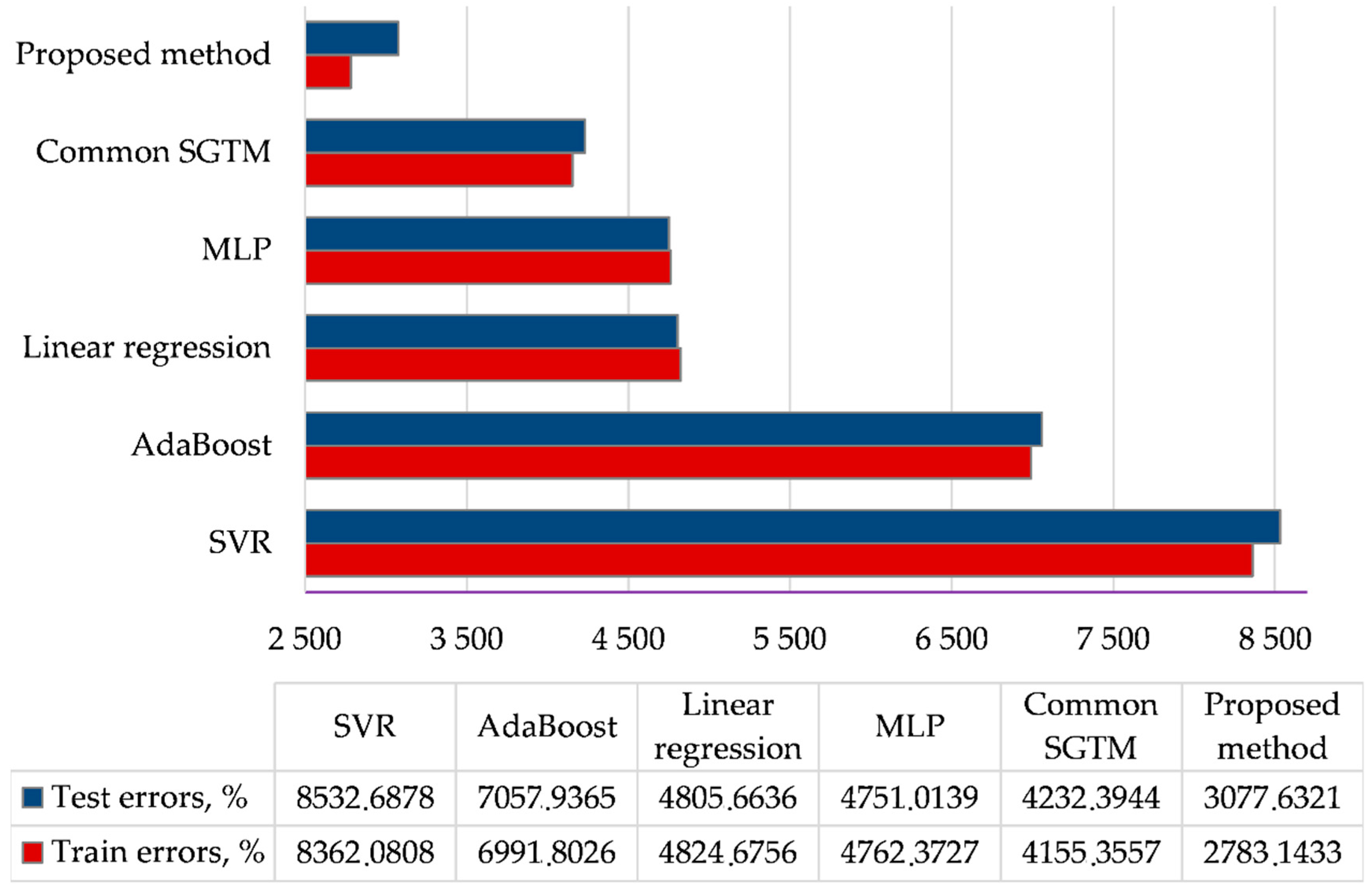
The results of the developed method (optimize version) were compared with the results of the known methods [6], which are demonstrated in Figure 6.

Figure 6 demonstrates the training and testing errors for all methods. As can be seen from the figure, the common SGTM neural-like structure provides the lowest error value of the regression task among all known methods. However, the use of Ito decomposition can significantly improve the accuracy of the method in both modes of operation by 1.5 and 1.3 times, respectively. This is because the linear non-iterative SGTM neural-like structure provides an exact search for the coefficients of the Kolmogorov–Gabor polynomial. In addition, reducing the number of hidden layer’s neurons allows discarding components (members of a polynomial) that do not affect the result. In this way, an effective approximation procedure with great accuracy is carried out.

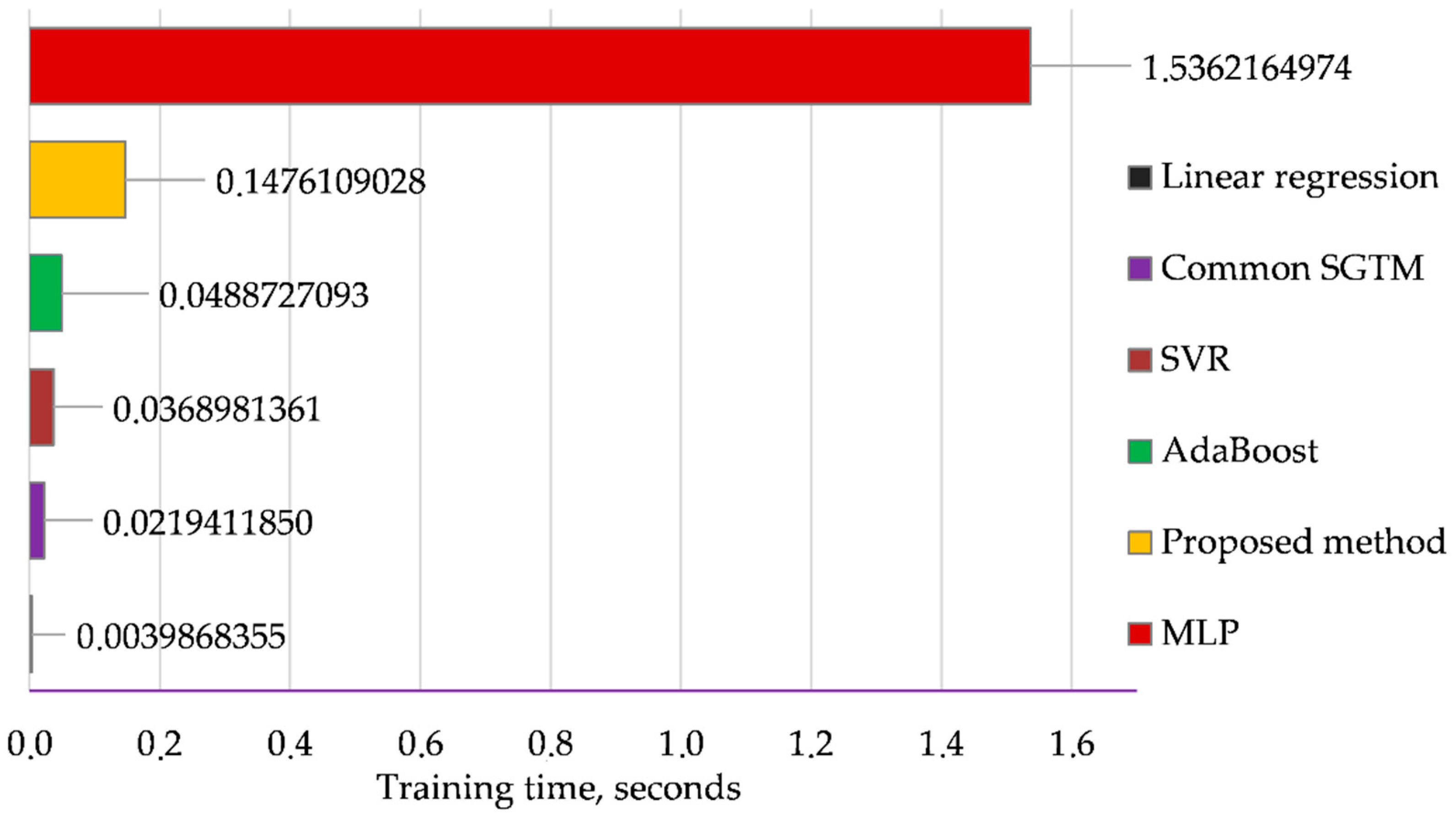
An important role in applying the computational intelligence methods for solving the practical tasks of processing large data arrays is played an important role for the duration of the training procedure. That is why in this work, the comparison of the training procedure duration for all considered methods is given. Figure 7 demonstrates the results of this investigation.

As can be seen from Figure 7, the multi-layered perceptron demonstrates the longest training time. The linear common SGTM neural-like structure provides one of the best results and is inferior only to linear regression. However, the latter method demonstrates poor results in accuracy (Figure 7). The developed method demonstrates 10 times faster training compared with multi-layer perceptron and less than 8 times slower training compared with the common SGTM neural-like structure. Obviously, the working time of the developed method has increased, as the dimension of the input space due to the use of Ito decomposition in accordance to equation (2) has significantly increased. However, the developed method demonstrates the best results both in the accuracy of work and in relation to the generalization properties of the chosen instrument of computational intelligence.

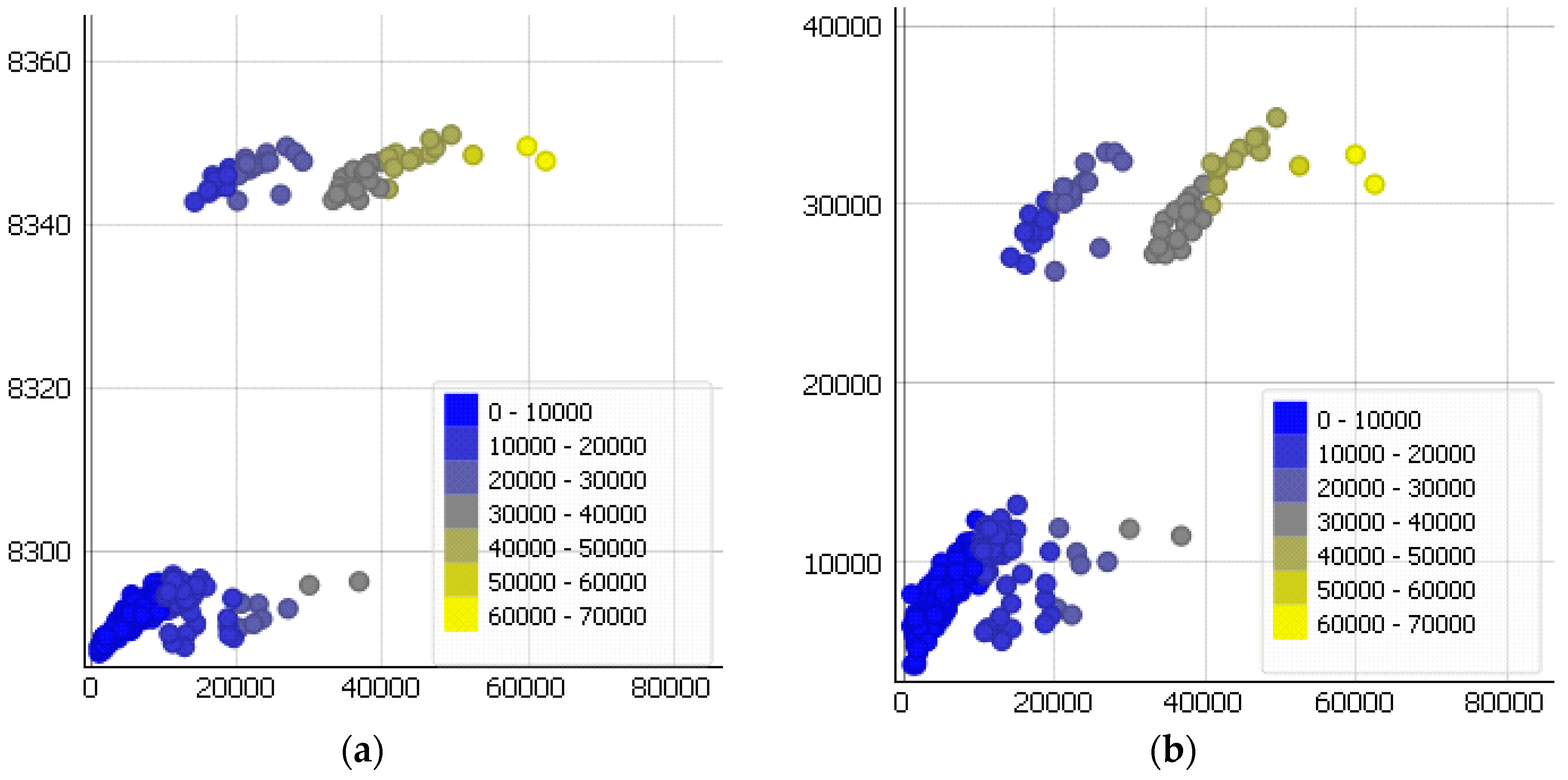
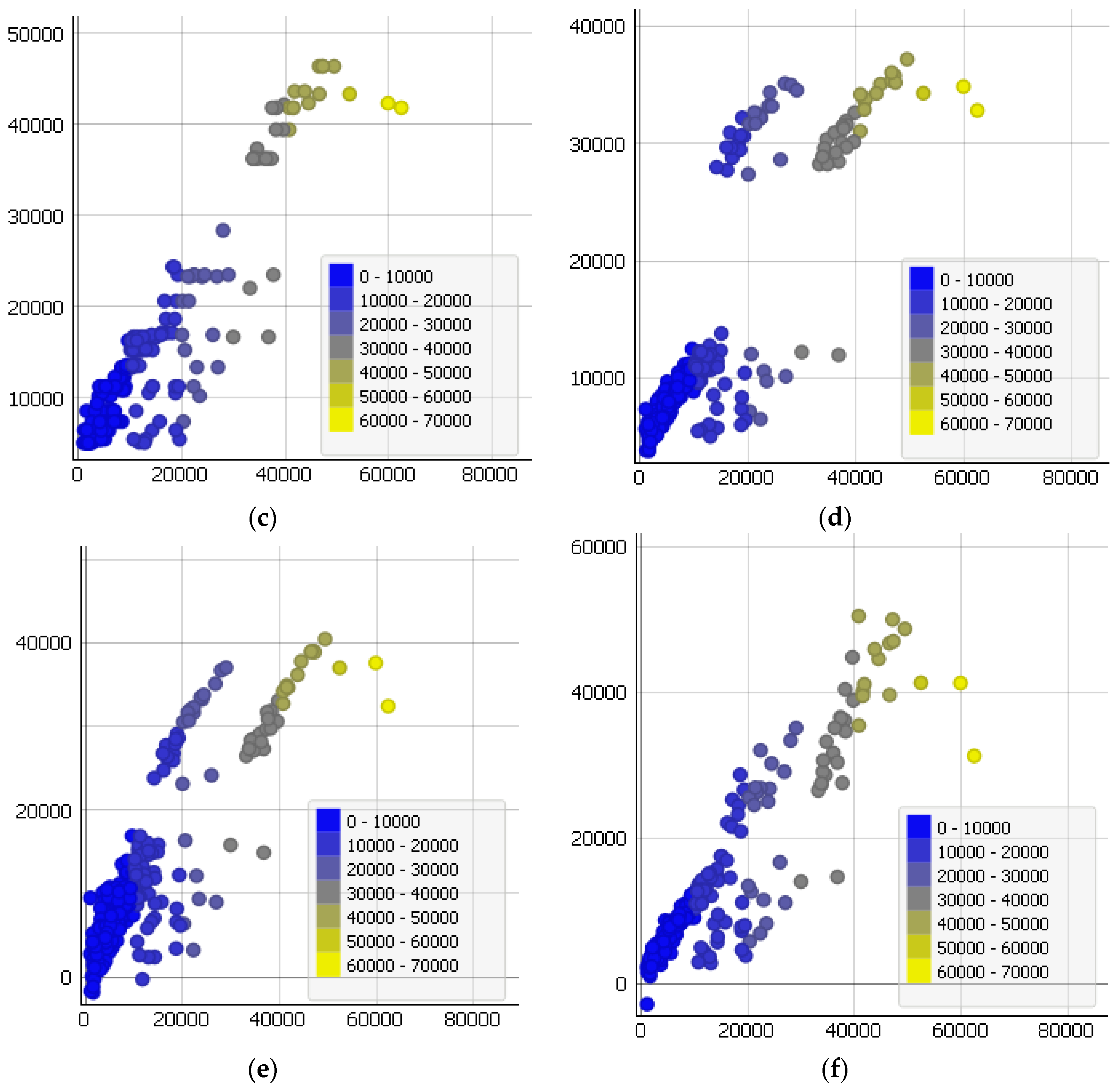
Figure 8 illustrates the visualization of the work for all investigated methods in the form of scatter plots. Figure 8f confirms the best results of the developed method among those considered as to the accuracy of its work.

This approach can be used for solving different task in Service Science area [32,33].

6. Conclusions

The authors describe the new developed non-iterative computational intelligence tool for solving the regression task in this paper. It combines the Ito decomposition and the neural-like structure of the successive geometric transformations model. The simulation was conducted to solve the individual medical cost prediction task. The effectiveness of the proposed tool is confirmed by comparing its work with existing predictors. The precision of the developed predictor shows the highest values based on five indicators: MAPE, SSE, SMAPE, RMSE, and MAE, in training and testing modes. In addition, a comparison between the training procedure duration of the developed tool with that of the existing ones was made. It demonstrates the satisfactory results of the experiment given the significant increase in the dimensions of the input data (from 11 to 77 input characteristics).

Based on the above, we can distinguish the following advantages of the developed predictor:

―: the quick, non-iterative training procedure;
―: the increase of generalization properties;
―: the significant increase in the prediction accuracy.

All these advantages give grounds to assert about the possibility of using the proposed instrument for solving the regression task in various fields, under conditions of both large and small data samples.

Further work will be conducted in the direction of the applying of the higher order’s Ito decomposition. Such an approach shall be effective by replacing the primary inputs of the task with the principal components, and by discarding the principal components with small variance values. The SGTM neural-like structure gives the fastest solution for obtaining the values that are very close to the principal components of each input vector.

Author Contributions

Conceptualization, R.T.; methodology, I.I.; software, P.V.; validation, R.T. and O.P.; formal analysis, R.T.; investigation, I.I.; writing—original draft preparation, I.I.; writing—review and editing R.T.; visualization, I.I. and N.L.; supervision, R.T.

Funding

This research received no external funding.

Acknowledgments

The authors thank the organizers of the DSMP’2018 conference for the opportunity to publish the article, as well as reviewers for the relevant comments that helped to better present the paper’s material.

Conflicts of Interest

The authors declare no conflict of interest.

Appendix A

Table A1. Training and testing errors of the developed method’s results when changing the number of neurons in the hidden layer: Mean Absolute Percentage Error (MAPE), Sum Square Error (SSE), Symmetric Mean Absolute Percentage Error (SMAPE), Root Mean Square Error (RMSE), Mean Absolute Error (MAE).

Observation/Indicator		Training Errors					Test Errors
Hidden Layer’s Neurons Number	Training Time	MAPE	SSE	SMAPE	RMSE	MAE	MAPE	SSE	SMAPE	RMSE	MAE
5	0.0328	98.0907	250,153.1643	0.2277	7647.4054	6017.2457	90.4530	122,496.0430	0.2134	7482.6368	5799.5606
10	0.0640	29.6955	199,827.0208	0.1463	6108.8903	3866.1687	30.6628	100,543.3525	0.1511	6141.6628	4033.6993
15	0.0774	36.0616	192,268.2087	0.1466	5877.8106	3873.7426	36.6546	96,848.9924	0.1486	5915.9938	3947.6894
20	0.0940	36.1080	191,597.2658	0.1466	5857.2993	3875.0551	36.3794	95,882.4545	0.1484	5856.9531	3937.6843
25	0.1231	37.2211	188,909.5383	0.1454	5775.1331	3842.2482	38.8044	95,367.0315	0.1483	5825.4686	3948.9449
30	0.1342	27.6548	156,156.1666	0.1085	4773.8333	2867.1614	29.0845	83,439.0789	0.1190	5096.8530	3185.9151
35	0.1476	27.0794	153,613.4998	0.1053	4696.1017	2783.1433	28.2033	82,337.1565	0.1149	5029.5423	3077.6321
40	0.1780	27.6964	152,671.6923	0.1053	4667.3098	2783.8583	30.0943	82,309.9318	0.1158	5027.8793	3103.5243
45	0.2000	27.8937	152,665.2744	0.1054	4667.1136	2786.0303	30.3035	82,387.0573	0.1161	5032.5905	3111.7831
50	0.2079	28.5096	152,568.5949	0.1054	4664.1580	2785.5579	30.6519	82,189.3916	0.1159	5020.5162	3107.0487
55	0.2719	28.5293	152,511.9680	0.1053	4662.4269	2783.5739	30.9454	82,394.3576	0.1162	5033.0364	3112.8836
60	0.2870	28.6878	152,374.2804	0.1053	4658.2177	2784.8075	30.6126	82,389.5643	0.1155	5032.7436	3092.6906
65	0.3159	28.6454	152,239.3691	0.1051	4654.0933	2779.0867	30.7230	82,638.1576	0.1158	5047.9289	3098.5853
70	0.3534	28.5060	151,938.2782	0.1049	4644.8887	2774.0156	30.9568	82,804.6760	0.1161	5058.1006	3105.5370
75	0.3537	28.3622	151,865.9138	0.1048	4642.6765	2769.1590	30.9699	82,795.9130	0.1160	5057.5653	3103.7871
77	0.3632	28.4187	151,771.1717	0.1047	4639.7801	2767.6075	30.8230	82,676.2620	0.1158	5050.2565	3099.7172

References

Melnykova, N.; Shakhovska, N.; Sviridova, T. The personalized approach in a medical decentralized diagnostic and treatment. In Proceedings of the 14th International Conference: The Experience of Designing and Application of CAD Systems in Microelectronics (CADSM), Lviv, Ukraine, 21–25 February 2017; Lviv Publishing House: Lviv, Ukraine, 2017; pp. 295–297. [Google Scholar]
Babichev, S.; Kornelyuk, A.; Lytvynenko, V.; Osypenko, V. Computational analysis of microarray gene expression profiles of lung cancer. Biopolym. Cell 2016, 32, 70–79. [Google Scholar] [CrossRef]
Medical Cost Personal Datasets. Insurance Forecast by Using Linear Regression. Available online: https://www.kaggle.com/mirichoi0218/insurance/kernels (accessed on 20 September 2018).
Bodyanskiy, Y.; Vynokurova, O.; Pliss, I.; Setlak, G.; Mulesa, P. Fast learning algorithm for deep evolving GMDH-SVM neural network in data stream mining tasks. In Proceedings of the 2016 IEEE First International Conference on Data Stream Mining & Processing (DSMP), Lviv, Ukraine, 21–25 August 2016; Lviv Publishing House: Lviv, Ukraine, 2016; pp. 257–262. [Google Scholar] [CrossRef]
Veres, O.; Shakhovska, N. Elements of the formal model big date. In Proceedings of the XI International Conference on Perspective Technologies and Methods in MEMS Design (MEMSTECH), Lviv, Ukraine, 2–6 September 2015; Lviv Publishing House: Lviv, Ukraine, 2015; pp. 81–83. [Google Scholar] [CrossRef]
Vitynskyi, P.; Tkachenko, R.; Izonin, I.; Kutucu, H. Hybridization of the SGTM Neural-like Structure through Inputs Polynomial Extension. In Proceedings of the 2018 IEEE Second International Conference on Data Stream Mining & Processing (DSMP), Lviv, Ukraine, 21–25 August 2018; Lviv Polytechnic Publishing House: Lviv, Ukraine, 2018; pp. 386–391. [Google Scholar]
Setlak, G.; Bodyanskiy, Y.; Vynokurova, O.; Pliss, I. Deep evolving GMDH-SVM-neural network and its learning for Data Mining tasks. In Proceedings of the 2016 Federated Conference on Computer Science and Information Systems (FedCSIS), Gdansk, Poland, 11–14 September 2016; pp. 141–145. [Google Scholar]
Hu, Z.; Bodyanskiy, Y.V.; Tyshchenko, O.K. A Cascade Deep Neuro-Fuzzy System for High-Dimensional Online Possibilistic Fuzzy Clustering. In Proceedings of the XI-th International Scientific and Technical Conference “Computer Science and Information Technologies” (CSIT 2016), Lviv, Ukraine, 6–10 September 2016; Lviv Polytechnic Publishing House: Lviv, Ukraine, 2016; pp. 119–122. [Google Scholar]
Ganovska, B.; Molitoris, M.; Hosovsky, A.; Pitel, J.; Krolczyk, J.B. Design of the model for the on-line control of the AWJ technology based on neural networks. Indian J. Eng. Mater. Sci. 2016, 23, 279–287. [Google Scholar]
Gajewski, J.; Valis, D. The determination of combustion engine condition and reliability using oil analysis by MLP and RBF neural networks. Tribol. Int. 2017, 115, 557–572. [Google Scholar] [CrossRef]
Hu, Z.; Jotsov, V.; Jun, S.; Kochan, O.; Mykyichuk, M.; Kochan, R.; Sasiuk, T. Data science applications to improve accuracy of thermocouples. In Proceedings of the 2016 IEEE 8th International Conference on Intelligent Systems (IS), Sofia, Bulgaria, 4–6 September 2016; pp. 180–188. [Google Scholar] [CrossRef]
Koprowski, R.; Lanza, M.; Irregolare, C. Corneal power evaluation after myopic corneal refractive surgery using artificial neural networks. BioMed. Eng. Online 2016, 15. [Google Scholar] [CrossRef] [PubMed]
Glowacz, A. Acoustic based fault diagnosis of three-phase induction motor. Appl. Acoust. 2018, 137, 82–89. [Google Scholar] [CrossRef]
Deng, L.; Yu, D. Deep Learning: Methods and Applications. Found. Trends Signal Process. 2014, 7, 1–199. [Google Scholar] [CrossRef]
Bellazzia, R.; Zupan, B. Predictive data mining in clinical medicine: Current issues and guidelines. Int. J. Med. Inform. 2008, 77, 81–97. [Google Scholar] [CrossRef] [PubMed]
Caruana, R. An empirical comparison of supervised learning algorithms. In Proceedings of the 23rd International Conference on Machine Learning, Pittsburgh, PA, USA, 25–29 June 2006; pp. 161–168. [Google Scholar]
Medical Cost Personal Datasets. Available online: https://www.kaggle.com/mirichoi0218/insurance (accessed on 9 September 2018).
Demsar, J.; Curk, T.; Erjavec, A.; Gorup, C.; Hocevar, T.; Milutinovic, M.; Mozina, M.; Polajnar, M.; Toplak, M.; Staric, A.; et al. Orange: Data Mining Toolbox in Python. J. Mach. Learn. Res. 2013, 14, 2349–2353. [Google Scholar]
Tkachenko, R.; Izonin, I. Model and Principles for the Implementation of Neural-Like Structures based on Geometric Data Transformations. In Advances in Computer Science for Engineering and Education; Advances in Intelligent Systems and Computing; Hu, Z.B., Petoukhov, S., Eds.; Springer: Cham, Swizland, 2018; Volume 754, pp. 578–587. [Google Scholar] [CrossRef]
Tkachenko, R.; Tkachenko, P.; Izonin, I.; Tsymbal, Y. Learning-Based Image Scaling Using Neural-Like Structure of Geometric Transformation Paradigm. In Advances in Soft Computing and Machine Learning in Image Processing; Hassanien, A., Oliva, D., Eds.; Studies in Computational Intelligence; Springer: Cham, Swizland, 2018; Volume 730, pp. 537–567. [Google Scholar] [CrossRef]
Weierstrass, K. Uber Die Analytische Darstellbarkeit Sogenannter Willkurlicher Funktionen einer Reellen Veranderlichen; Sitzungsberichte der Akademie der Wissenschaften: Berlin, Germany, 1885; pp. 633–639. [Google Scholar]
Iba, H.; Sato, T. Meta-level Strategy for Genetic Algorithms Based on Structured Representations. In Proceedings of the Second Pacific Rim International Conference on Artificial Intelligence, Seoul, Korea, 15–18 September 1992; pp. 548–554. [Google Scholar]
Iba, H.; Sato, T.; Garis, H. System Identification Approach to Genetic Programming. In Proceedings of the First IEEE Conference on Evolutionary Computation, Orlando, FL, USA, 27–29 June 1994; Volume I, pp. 401–406. [Google Scholar]
Ivakhnenko, A.G. Polynomial Theory of Complex Systems. IEEE Trans. Syst. Man Cybern. 1971, 1, 364–378. [Google Scholar] [CrossRef]
Kargupta, H.; Smith, R.E. System Identification with Evolving Polynomial Networks. In Proceedings of the Fourth International Conference on Genetic Algorithms, San Mateo, CA, USA, 14–17 September 1991; pp. 370–376. [Google Scholar]
Nikolaev, N.I.; Iba, H. Accelerated Genetic Programming of Polynomials. Genet. Program. Evol. Mach. 2001, 2, 231–257. [Google Scholar] [CrossRef]
Haykin, S. Neural Networks and Learning Machines, 3rd ed.; Pearson Education, Inc.: London, UK, 2009; p. 904. [Google Scholar]
Ng, A. Machine Learning. Lecture 7.1 Regularization. The Problem of Overfitting. Available online: https://www.youtube.com/watch?v=u73PU6Qwl1I (accessed on 9 September 2018).
Korobchynskyi, M.V.; Chyrun, L.B.; Vysotska, V.A.; Nych, M.O. Matches prognostication features and perspectives in cybersport. Radio Electron. Comput. Sci. Control 2017, 95–105. [Google Scholar] [CrossRef]
Botchkarev, A. Performance Metrics (Error Measures) in Machine Learning Regression, Forecasting and Prognostics: Properties and Typology. 2018. Available online: https://arxiv.org/abs/1809.03006 (accessed on 9 September 2018).
Chen, C.; Twycross, J.; Garibaldi, J.M. A new accuracy measure based on bounded relative error for time series forecasting. PLoS ONE 2017, 12, 54–67. [Google Scholar] [CrossRef] [PubMed]
Molnár, E.; Molnár, R.; Kryvinska, N.; Greguš, M. Web Intelligence in practice. J. Serv. Sci. Res. 2017, 6, 149–172. [Google Scholar] [CrossRef]
Kryvinska, N. Building Consistent Formal Specification for the Service Enterprise Agility Foundation. J. Serv. Sci. Res. 2012, 4, 235–269. [Google Scholar] [CrossRef]

Figure 1. Dataset visualization using Orange Software, version 3.13.0. The x-axis represents the insurance contractor’s age, and the y-axis is the size of the medical insurance costs. The circles mark women, and the crosses mark men. The blue circles mark the woman-non-smoker, and the red circles mark the woman-smoker. The blue crosses mark the male-smoker, the red crosses mark the male non-smoker. The size of the figures reflects the value of the body mass index. The larger index, the larger shape of the corresponding figure. Shapes and colors were chosen randomly.

Figure 2. Topology of the common linear neural-like structure of the successive geometric transformations model (SGTM).

Figure 3. Topology of the proposed model (combining the use of the Ito decomposition and SGTM linear neural-like structure).

Figure 4. Optimal parameters identification for training and test modes: (a) mean absolute percentage error (MAPE) value according to changing the hidden layer’s neurons number, (b) MAPE value according to changing the training time.

Figure 5. Topology of the proposed optimized model.

Figure 6. Mean absolute error (MAE) in training and testing modes for developed and existing methods. On the x-axis, the mean absolute error value for all considered methods is illustrated.

Figure 7. The training time for all methods.

Figure 8. Visualization of the methods’ results. On the x-axis, the real values of insurance medical costs are given, and on the y-axis are values obtained by one of the methods: (a) support vector regression with RBF kernel, (b) linear regression, (c) adaptive boosting, (d) multilayer perceptron, (e) linear common SGTM neural-like structure, or (f) proposed method.

Table 1. Original dataset.

#	Insurance Contractor Age	Insurance Contractor Gender	Body Mass Index, kg/m²	Number of Dependents	Smoking	Beneficiary’s Residential Area in the United States	Individual Insurance Costs
1	19	female	27.9	0	yes	southwest	16,884.924
2	18	male	33.77	1	no	southeast	1725.5523
3	28	male	33	3	no	southeast	4449.462
4	33	male	22.705	0	no	northwest	21,984.4706
5	32	male	28.88	0	no	northwest	3866.8552
6	31	female	25.74	0	no	northeast	3756.6216
…	…	…	…	…	…	…	…
i	60	female	27.9	0	yes	southwest	16,884.924
…	…	…	…	…	…	…	…
n	61	female	29.07	0	yes	northwest	29,141.3603

Table 2. Prepared Dataset. F—female; M—male; BMI—body mass index; ICC—individual insurance costs.

#	Age	F	M	BMI, kg/m²	Children	Smoker	Non-Smoker	Area 1	Area 2	Area 3	Area 4	IIC
1	19	1	0	27.9	0	1	0	1	0	0	0	16,884.924
2	18	0	1	33.77	1	0	1	0	1	0	0	1725.5523
3	28	0	1	33	3	0	1	0	1	0	0	4449.462
4	33	0	1	22.705	0	0	1	0	0	1	0	21,984.471
5	32	0	1	28.88	0	0	1	0	0	0	1	3866.8552
6	31	1	0	25.74	0	0	1	0	0	1	0	3756.6216
…	…	…	…	…	…	…	…	…	…	…	…	…
i	60	1	0	27.9	0	1	0	1	0	0	0	16,884.924
…	…	…	…	…	…	…	…	…	…	…	…	…
n	61	0	0	29.07	0	1	0	0	0	1	0	29,141.360

Table 3. Modeling results based on mean absolute percentage error (MAPE), sum square error (SSE), symmetric mean absolute percentage error (SMAPE), root mean square error (RMSE), and mean absolute error (MAE) in training and test modes. SGTM—successive geometric transformations model.

Method/Indicator	MAPE	SSE	SMAPE	RMSE	MAE
Training errors
Proposed model (SGTM + Ito decomposition)	28.4187	151,771	0.1047	4639.78	2767.61
Proposed model with optimal parameters	27.0794	153,613	0.10531	4696.1	2783.14
Test errors
Proposed model (SGTM + Ito decomposition)	30,823	82,676	0.1158	5050.3	3099.7
Proposed model with optimal parameters	28,203	82,337	0.1149	5029.5	3077.6

© 2018 by the authors. Licensee MDPI, Basel, Switzerland. This article is an open access article distributed under the terms and conditions of the Creative Commons Attribution (CC BY) license (http://creativecommons.org/licenses/by/4.0/).

Share and Cite

MDPI and ACS Style

Tkachenko, R.; Izonin, I.; Vitynskyi, P.; Lotoshynska, N.; Pavlyuk, O. Development of the Non-Iterative Supervised Learning Predictor Based on the Ito Decomposition and SGTM Neural-Like Structure for Managing Medical Insurance Costs. Data 2018, 3, 46. https://doi.org/10.3390/data3040046

AMA Style

Tkachenko R, Izonin I, Vitynskyi P, Lotoshynska N, Pavlyuk O. Development of the Non-Iterative Supervised Learning Predictor Based on the Ito Decomposition and SGTM Neural-Like Structure for Managing Medical Insurance Costs. Data. 2018; 3(4):46. https://doi.org/10.3390/data3040046

Chicago/Turabian Style

Tkachenko, Roman, Ivan Izonin, Pavlo Vitynskyi, Nataliia Lotoshynska, and Olena Pavlyuk. 2018. "Development of the Non-Iterative Supervised Learning Predictor Based on the Ito Decomposition and SGTM Neural-Like Structure for Managing Medical Insurance Costs" Data 3, no. 4: 46. https://doi.org/10.3390/data3040046

Article Menu

Development of the Non-Iterative Supervised Learning Predictor Based on the Ito Decomposition and SGTM Neural-Like Structure for Managing Medical Insurance Costs^†

Abstract

1. Introduction