Measuring and Linking the Missing Part of Biodiversity and Ecosystem Function: The Diversity of Biotic Interactions


Red de Ecoetología, Instituto de Ecología AC, Xalapa, Veracruz 91073, Mexico
*
Author to whom correspondence should be addressed.
Diversity 2020, 12(3), 86; https://doi.org/10.3390/d12030086
Submission received: 5 December 2019
/
Revised: 7 February 2020
/
Accepted: 9 February 2020
/
Published: 25 February 2020
(This article belongs to the Special Issue Symbioses and the Biodiversity-Ecosystem Function Relationship)
Abstract
:Biotic interactions are part of all ecosystem attributes and play an important role in the structure and stability of biological communities. In this study, we give a brief account of how the threads of biotic interactions are linked and how we can measure such complexity by focusing on mutualistic interactions. We start by explaining that although biotic interactions are fundamental ecological processes, they are also a component of biodiversity with a clear α, β and γ diversity structure which can be measured and used to explain how biotic interactions vary over time and space. Specifically, we explain how to estimate the α-diversity by measuring the properties of species interaction networks. We also untangle the components of the β-diversity and how it can be used to make pairwise comparisons between networks. Moreover, we move forward to explain how local ecological networks are a subset of a regional pool of species and potential interactions, γ-diversity, and how this approach allows assessing the spatial and temporal dynamics of ecological networks. Finally, we propose a new framework for studying interactions and the biodiversity–ecosystem function relationship by identifying the unique and common interactions of local networks over space, time or both together.
1. Introduction
Since the first observations and studies by modern naturalists, biologists have recognized that interactions between individuals of different species are the building blocks of ecosystems and ecological communities [1,2]. Interactions between species’ individuals are part of all ecosystem attributes, from primary productivity to population dynamics, and play an important role in the structure and stability of biological communities [3]. Over evolutionary time, major breakthroughs that have increased the diversity of species are also associated with an increase in the diversity and complexity of species interactions. For instance, early emerging bacteria started to interact with each other and evolved by endosymbiosis, which in turn generated more complex life forms, the eukaryotes [4]. The rise of angiosperms more than 110 million years ago has also been related to an increasing number of interactions with a great diversity of animals, such as pollinators and seed-dispersers [5,6]. However, pollination can be traced back to pre-angiosperm floras as there is growing evidence that angiosperms evolved in habitats in which many gymnosperms were pollinated by insects [7]. Although the rise of life in its diverse forms had been understood in light of interactions between species, however, it was not until the 1970s that ecologists started to focus closely on such components of biodiversity [2,6].
In general, biodiversity is understood as the complexity of life forms and their direct and indirect relationships, and species interactions therefore play a role in many ecological and evolutionary processes [3]. For example, in the tropics nearly 90% of plants require animals (i.e., mutualistic partners) to complete their life cycles, including pollinators and seed-dispersers [7,8]. In recent years, however, the diversity and ecological processes related to interactions between species have been threatened by lost habitat, climate change and biological invasions [9,10,11]. We must also take into account that when a species becomes extinct in an ecosystem, all ecological functions related to its biotic interactions may also be lost [12]. For instance, the extinction of bird seed dispersers or bee pollinators could lead to the loss of their vital ecological functions: plant reproduction and dispersal in the environment [13]. The loss of interactions can also limit the dispersal of genes across different regions, having negative effects on populations on large scales and ultimately accelerating the extinction of species [14]. The previous examples show that interactions are indeed biological processes that affect species diversity, including the dynamics and functioning of ecosystems; however, such studies have mainly focused on showing biotic interactions as a process and not as a component of biodiversity.
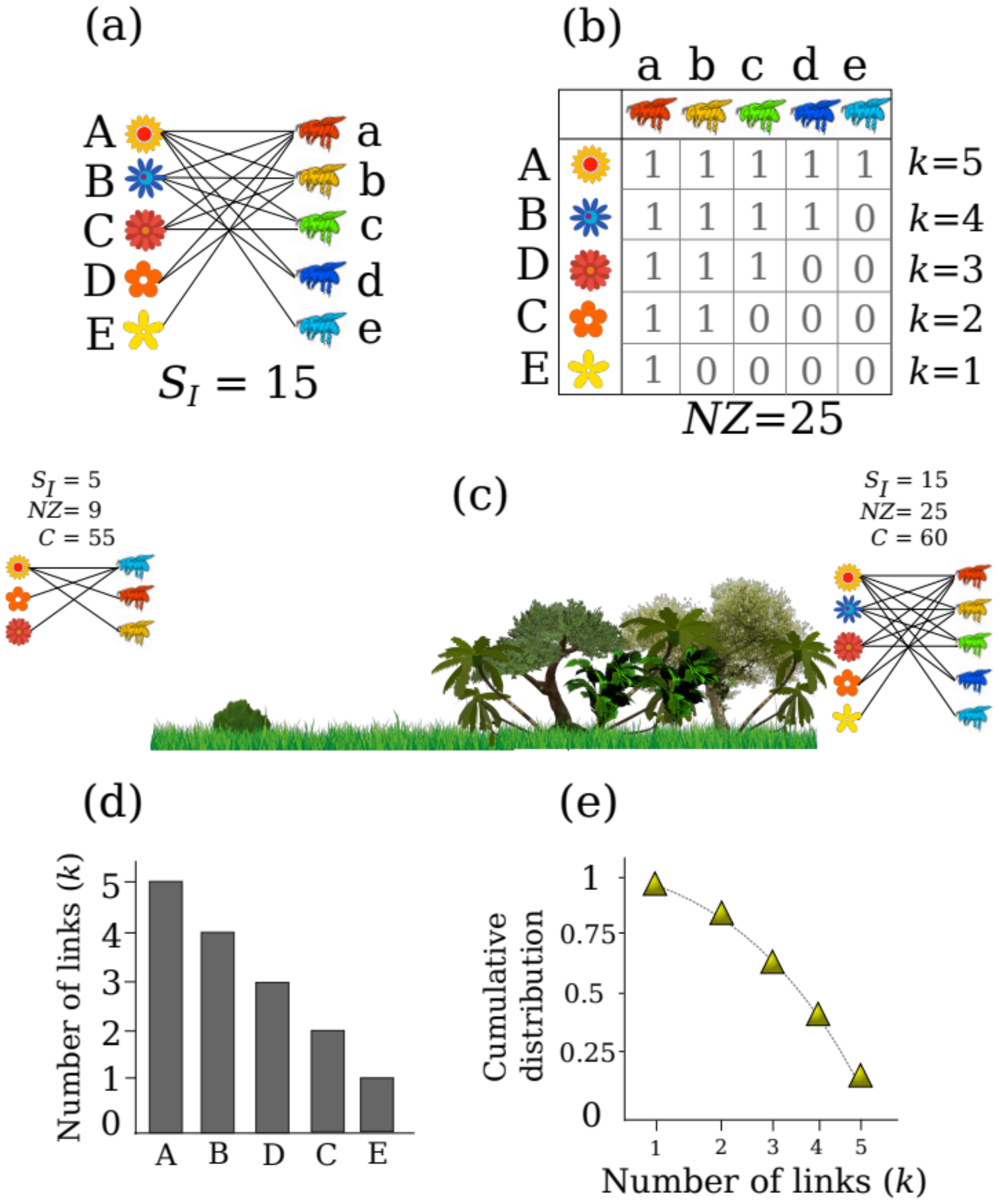
Traditionally, studies of species interactions have focused on the interactions of single taxa, such as the floral visitors of one plant species (e.g., [15]), or only between pairs of species (e.g., [16]), however, species are not isolated entities in nature and along a spatio-temporal gradient they are embedded within a large and complex interaction network [17]. The idea that species are embedded in large and complex networks is not new [1], however it was not until recent decades that ecologists started to describe such complexity as ecological networks [2]. An ecological network is a mathematical and conceptual representation of both species and their interactions, and provides an integrated representation of ecological communities [18]. In these ecological networks, species are depicted as nodes, and their interactions are depicted by links describing, for instance, the use of plants as resources by animals (Figure 1a). This is achieved by recording interactions between individuals of the same or different species (e.g., whether the individual of species A interacted with the individual of species a, Figure 1b) and using the information to further fill matrices with binary data (i.e., if the interaction is observed 1, if not 0) or weighted data (i.e., the number of times each individual was observed interacting, such as the number of times a bee visits a certain flower; [19]). In general, ecological networks represent the interactions of two trophic levels (i.e., bipartite networks), such as plants and their floral visitors, seeds and their animal dispersal agents or even interactions between individuals at the same trophic levels, such as plant facilitation interactions [20,21]. Although the study of bipartite networks has increased our knowledge and understanding of the diversity of interactions, the study of complete sets of interacting species involving multiple interaction types (e.g., different types of mutualisms in a single network: pollination, seed dispersal and ant defensive systems [22]) is still at the frontier of the study of interactions. By studying ecological networks, we can measure and describe how the individuals of different species interact; for example, their interaction diversity, structural organization or trophic specialization. The development of ecological network descriptors has prompted a renewed interest in understanding how and why species and their interactions vary across both space and time [23,24]. These descriptors allow us to compare the interactions of the same or different types (i.e., pollination vs seed dispersal networks), across environments and geography by describing the variation and the drivers of its diversity, structural organization or trophic specialization [24,25]. We can thus measure, for example, how the diversity of pollination interactions varies across latitude or habitats with different precipitation regimes [26,27,28].
Analyzing interactions across space and time has established that interaction networks are dynamic and have a structured variation in α, β and γ diversity, not only because we can record different species interacting across spatio-temporal gradients but also because the same species will interact in different ways over such gradients [25,29]. The idea that interactions have α, β and γ diversity is relatively new, and consequently poorly understood [25]. The term “diversity of species interactions” had already been used in the early 2000s to highlight its importance for the origin, maintenance, function and conservation of biodiversity [27,30]. However, despite the potential use of “diversity of interactions” as a component of biodiversity that can be measured and that varies across environmental gradients, the amount of theoretical and empirical information available is still limited in the literature [31] (but see [29], for beta diversity of interactions). The lack of knowledge and the misunderstanding about the diversity of interactions could be related to the fact that many ecological theories and hypotheses avoid or minimize biotic interactions as a potential driver of the origin, maintenance and distribution of biodiversity [32,33]. If ecological interactions are considered in such explanations, its role maintaining or explaining biodiversity is not measured and it is merely anecdotal (e.g., Eltonian noise hypothesis [33,34]). In other cases, we have seen that when the diversity of interactions is measured it is not properly interpreted due to the novelty of these ideas and methods, or it is measured following a series of instructions without thinking about the meaning of such measures (see [35]). The main objective of this work is to explain our basic knowledge about the diversity of interactions involving two trophic levels (e.g., plant-pollinator and plant-disperser), and how (i) it is measured; (ii) such measures should be biologically interpreted; and (iii) this knowledge is useful for both ecological theory and conservation applications. We start by explaining the local diversity of interactions (α-diversity) and then discuss how to measure the turnover of species interactions over space and time (β-diversity), and we will conclude with how to measure regional pools of species interactions (γ-diversity).
2. Measuring Local Diversity of Interactions (α-Diversity)
If we want to measure the local diversity of interactions between two habitats, or between seasons, or even across the months of a year, whatever the case is, we have to start by measuring the number of different interactions realized in each case; this is interaction richness (SI = number of links/interactions between species, Figure 1a). This measure gives us a first glance at how many interactions are realized in the observed community, without taking into account the number of species, as this is just an interaction-centered measure, analogous to species richness [30]. In this and further sections, we will use the terms “realized” or “potential” interactions, as interactions have to pass ecological filters to actually occur. This is contrary to the common assumption that species will interact whenever they co-occur, and current knowledge supports the idea that interactions are filtered, and thus the co-occurrence of species is not the only predictor of the realization of interactions [24,25]. When we measure the number of realized interactions in a certain habitat or period of time, we have to acknowledge that interaction richness can be measured in two distinct forms. These can be understood in the context where one individual of a species can establish: (i) different types of interactions and (ii) different interactions of the same type. For example, one tree can establish interactions with five pollinators, which represent five different interactions of the same type (first type of interaction richness; Figure 1a), whereas the same tree may also establish interactions with herbivores, frugivores, mycorrhizae and parasites, and thus the type of interactions is itself another kind of interaction richness, which can be described and measured.
Diversity is more than just species or interaction richness, and so interaction diversity can also be measured in terms of the number of species interacting in one network, rather than just describing the number of interactions within a network. For example, by comparing two communities, we can start by measuring its interaction richness along with the size of the network and its connectance. Network size (NZ) gives us a measure of the maximum number of observable interactions, and is calculated by multiplying the number of total species in each trophic level within a network (Figure 1b). Connectance is the percentage of the total number of potential interactions within a network that are actually realized, and is calculated using the following formula:
This descriptor ranges from 0 (no interactions are realized) to 100 (all potential interactions are realized). Both measures go beyond interaction richness and give us a description of the density of potential (NZ) and realized interactions (C). To make this more straight-forward, we can consider an example: imagine we have measured the interactions in a pasture and found that its interaction richness is SI = 5, and we compare it with a covered forest with SI = 15 (Figure 1c). This calculation is made by counting the number of unique interactions that have been recorded, in this case, the number of 1’s in the matrix (Figure 1b). By interpreting the calculated values we can start to see that one habitat has more realized interactions than another. Further, we find that our covered forest has a network size of 25 and our pasture of 9, this by multiplying the number of species (number of plants × animals) that are part of each network (e.g., three plants by three pollinators in the left side of Figure 1c). We can interpret that this indicates that there is a higher number of possible interactions in the covered forest than in the pasture. Possibly due the higher diversity of species that live in the covered forest. If we move forward to measure its connectance, however, we will see that in the covered forest the connectance reaches 60 and in the pasture it is 55, which shows that despite the differences in interaction richness and network size between both habitats, the number of realized interactions is quite similar. In the pasture and the covered forest more than half of the potential species interactions are realized, despite both networks having different sizes. Although there are more realized interactions in the pasture (i.e., higher connectance), the lower proportion of realized interactions in the covered forest could be explained by the differences in species richness between habitats. Following this, it is important to note that species richness affects the total of realized interactions, and such a bias has to be taken into account when examining interaction diversity, particularly connectance, see [35]. The previous example shows that simple calculations of the properties of ecological networks, based on the richness of interactions (i.e., binary data) and the number of species, can provide a description of the local diversity of interactions, something that is known by community ecologists as alpha diversity.
To truly understand such measures we encourage the reader to think of interactions as the entity to be measured, and to move forward to visualize communities as systems not only assembled by species, but by species related by links. The comparisons made in this first example are meant for didactic purposes, however, the reader must be aware that comparisons among networks should be made properly using null modeling or with an appropriate number of repetitions to use conventional statistics. The objective of a null model is to question the mechanism behind a pattern, and it works by deliberately removing a mechanism and showing whether removing it reproduces the pattern or not [36]. In ecological networks, null models are used to test whether the value of a descriptor calculated from empirical data is higher than that expected by random patterns of interaction [23]; for example, whether the observed interaction frequencies can be reproduced by a simple model without taking biological mechanisms into account [17].
In ecology, networks are built with groups of species and their interactions, and thus the effect of the number of interactions by species (e.g., how many flower species were visited by a bee species) can be used to describe the diversity of interactions [37]. In this sense, each species within a network establishes a number of links with other species; for example, one highly competitive bee species may establish five links, whereas one specialized bee species only establishes one or two links. Correspondingly, the number of links that each species establishes is called the degree, and in graph theory, it is noted as k. If we examine an interaction network, each species will display different degree frequencies (Figure 1b). In a network the degree of each species will vary, ranging from species which establish only one or two interactions (i.e., low degree), to species with many interactions (i.e., a high degree). In this way, the degree of each species is a measure of the generalization of the species (i.e., the number of resources used by each species). If we examine the distribution of the generalization of the species of a network, we will obtain a description of the interactions of a community of species (i.e., degree distribution plot). The degree distribution plot is analogous to a rank–abundance plot (i.e., Whittaker plot), but instead of species abundances, we plot the number of pairwise interactions of each species (Figure 1d). As a result, the distribution of the interactions in a given community show us that mutualistic networks are not randomly assembled [38]. Because when we plot and measure the cumulative distribution of the degree of species from different habitats with different evolutionary histories, we will find that a pattern arises. In the majority of cases, the cumulative distribution of the degree of the species will follow, or can be predicted by, truncated power-laws [30,38]. This is similar to what happens when we measure the distribution of the relative abundance of the species in different habitats; the distribution of species abundances will show log-normal or zero-sum distributions [39] because ecological communities are commonly assembled by few very abundant species and many rare species (singletons) no matter the identity and evolutionary history of the habitat [39]. In ecological networks, the truncated power-law indicates that interactions follow a predictable distribution that is free of scale. This means that if we sample the interactions of one site properly, no matter how much effort we put into recording new interactions we will always find a continuum of few species with a great number of established interactions and many species with just a few interactions [38]. Notably, the shape of the degree distribution of interactions can be explained, in part, by current frameworks such as neutral theory, because it has been shown that nearly 60% to 70% of the observed interaction frequencies can be explained only by the neutral variation in the relative species abundances [40]. This means that abundant species should interact most frequently with each other and with less abundant species, while less abundant species will rarely interact among themselves [40]. This evidence indicates that theories explaining the interactions between species and the assembly of communities could be unified [41,42]. The remaining 30–40% of the variation in the distribution of interaction degree that is not explained by the neutral assembly of communities, however, remains a frontier in the study of ecological interactions (but see [43,44]).
The previous techniques describe the diversity of interactions using interaction matrices that only include whether an interaction is realized or not; 1 if the interaction is realized and 0 otherwise. In this approach the same weight is given to all the links, which distorts the true picture of the diversity of the interactions, since free-living species interact quantitatively, generating a complex system of interactions, which allows the study of species preferences, for instance [19]. Further development of the theory of interaction networks has shown that indices such as connectance are extremely sensitive to different levels of sampling effort or network size [35]. Although they are useful in some cases (to compare networks of the same size and sampling effort), we recommend using approaches that take into account the bias generated by the sampling effort and network size, in order to drive clear conclusions and avoid erroneous interpretations of network indexes [45]. When we build ecological networks, we can also record the number of times we observe or detect one interaction; for example, how many times one hummingbird species visited a flower, or the times a bird ate a fruit of the same tree species. Using this approach we can calculate more elaborated indexes which take into account that not all species interact with the same frequencies [46]; such indexes are based on the Shannon entropy (H). In its purest form, H measures evenness, so for a given number of events H reaches its higher value when all events occur in equal proportions, however, this interpretation is not always made with the H index, because sometimes its higher values are interpreted as higher diversity per se. We can use several H derived indexes to measure the diversity of interaction networks. One of these measures how uniformly the interactions of one community are sorted, called Interaction evenness (ES), and it can be calculated with the following formula:
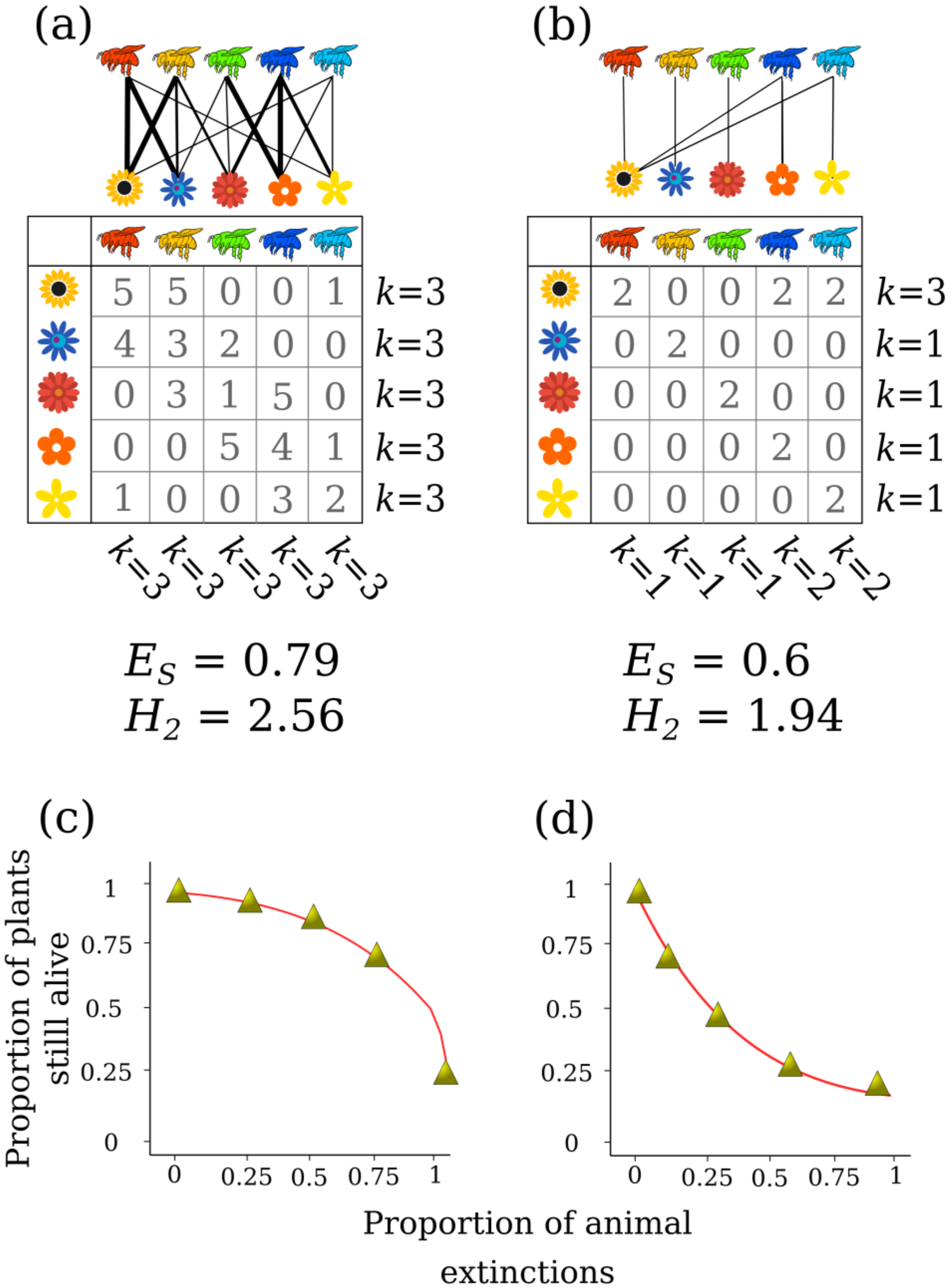
where pij is the proportion of the frequency of interactions in a network A. Network A is defined as aij = number of interactions between the higher trophic level i and the lower trophic level j. According to the logic of the H index, the higher the values obtained by this index, the more the interactions in the network are uniformly sorted, and the majority of species in the network establish the same number of links (Figure 2a). In this case, lower values indicate that interactions are more heterogeneously sorted, and the species in the network establishes different numbers of links (Figure 2b).
To estimate interaction diversity using H we need to consider that networks are formed of two trophic levels, and thus the calculation of the diversity of interactions considers the two dimensions of the matrix, the values in the columns and rows. This is different to the traditional H index used to measure the diversity of an ecological community, as this approach only considers the values in a single row of a matrix (i.e., one dimension). Interaction diversity is denoted as H2 to avoid confusion with its one-dimensional version H, and it can be calculated with the following formula:
where m represents the total frequency of interactions in a matrix aij. Indexes based on Shannon entropy describe the heterogeneity of the entries within a matrix, which can be used to characterize the diversity of associations based on interaction frequencies. The interpretation of the diversity of interactions H2 is straightforward, where higher values indicate that the majority of species establish more interactions (Figure 2a), whereas lower values of H2 indicate that the majority of species establish fewer interactions (Figure 2b). As these indexes are based on Shannon entropy, we have to acknowledge that they reflect the distribution of interactions of all the species in the networks, so its interpretation must be done at a network level, not a species level. It is worth noting that this index measures the heterogeneity of the interactions within a community but not necessarily its specialization; there are other indexes for such purposes that are designed to control the effects of neutrality in interaction frequencies, see [47].
Historically, theoretical studies have suggested that interactions are necessary to maintain biodiversity and ecosystem stability. However, conservation policies usually focus on preserving species and their diversity rather than its functional role [30,48]. Recently, conservation science has drawn attention to such bias, and has begun to shift towards conserving species and their functionality [48]. Ecological networks theory recognizes that some species contribute more to network stability (i.e., resilience to the extinction of species) than others, which suggests that not all species make significant contributions to the functioning of the ecosystem [22,30]. As already noted, ecological networks follow truncated power-laws in which most species are connected with a few links, and very few species are highly connected [26,38]. In general, networks that display power-laws present a characteristic response to the removal of nodes, and in the case of ecological networks to the extinction of species [30]. When a node is randomly removed from a network, in this case when a species goes extinct, the network exhibits high stability, meaning that the system remains cohesive (i.e., highly connected) and functional [30]. By contrast, if the highly connected species are removed, the connectivity of the whole system is affected, which eventually leads to the fragmentation of one network into many small networks [22]. Complex systems involve multiple interacting parts, and their behavior is determined by the sum of the interaction of all their parts and not by the behavior of their parts in isolation, and this is the case for ecological networks. Interaction networks are therefore resilient (i.e., they do not collapse) to the random extinction of species, however they are highly sensitive to the loss of highly connected species [49]. Using this approach, we can measure the robustness (R) of each of the two trophic levels of a network to the systematic removal of species [50,51]. This is calculated by estimating the area below the extinction curve after simulating the cumulative removal of species from a network (Figure 2c,d). Robustness values range from 0 (less robust network) to 1 (most robust network). This approach does not necessarily represent real extinctions in nature, but it gives us a tool for conservation purposes. Rare species are usually the first to become extinct in a network because they have low abundances, but the remaining species in a network will still have others with which to interact. For example, if a specialist pollinator becomes extinct, the plant species that it interacted with can still be pollinated by a generalist species. Highly connected species thus provide a buffer for the network against secondary extinctions, or phenology shifts generated by climate change [22,52]. In contrast, the loss of a highly connected species can be detrimental to rare species that depend on its services and even to whole network stability [30,49]. This is also relevant in the case of antagonistic interactions, for example, if a predator does not remove highly abundant seeds, the seeds of rare and less competitive species would not be able to establish in an environment dominated by one highly competitive plant species (i.e., invasive plants; [53]). It is worth mentioning that despite the potential use of network robustness (R) to evaluate the tolerance of interactive communities to species extinction, the amount of empirical information available is still limited and controversial in the literature. On the one hand, most theoretical studies have shown that when generalist species are experimentally removed from a community, its extinction curves rapidly decrease [54]. On the other hand, in an empirical study, when the generalist harvester ant species was locally extinct, other submissive ant species with fewer interactions replaced its generalist role in the community [55]. However, in a plant-pollinator system when highly visited plants were removed, pollination and insect foraging were jeopardized [56]. In addition, recent theoretical development has shown that sometimes extinction rates are not fast enough, so species have time to adapt and generate new links/interactions, and this means that the rules of the assembly of ecological networks include processes that increase the robustness of ecological networks [57]. Therefore, knowing the drivers of the different tolerances of interactive communities to species extinctions could improve our understanding of the dynamics of ecological interactions in a more comprehensive way [54]. In the light of conservation applications, we propose that strategies must be focused on preserving highly connected species, as they increase ecosystem functionality by encouraging resilience to the random extinction of species.
3. Measuring the Turnover of Species Interactions (β-Diversity)
Until now we have been describing and explaining how to measure the local diversity of interactions, however, local ecological networks are subsets of a regional pool of species and their potential interactions [25]. As species are filtered across space and time, their abundance and richness vary and, it is expected therefore that their interactions may also vary [24,25]. In this sense, the differences in their species composition between two local communities may generate variation in their interactions [58]. As we already mentioned, species do not interact whenever they co-occur, and interactions are filtered in order to be realized (e.g., phenology, body size and environmental conditions [24]). For example, when a phenological mismatch generates variation in the interaction networks between two habitats, one hypothetical scenario is that a bee species visits the same plant species in two habitats, but if in one habitat the plant is not producing flowers, the bee and the plant will never interact. If the plant is flowering in the other of our hypothetical habitats, this will generate differences in the realized interactions between habitats, through the filtration of one interaction. Because, the bee and its flower will interact in one habitat and in the other they will not; thus, how do we measure this variation generated by pairwise interactions at a network level, and how can we measure such variation across space and time?
These questions have found a response in recent years with the rise of new frameworks based on some old and new ideas. In the 2000s, when ecologists started to study ecological networks, they observed that interactions presented invariant topological properties, but they also observed that the interactions in the same place varied, in terms of species identities, from day-to-day, week-to-week and even from year-to-year [59]. Even though the same species were observed over time, the same species was shown to change their interaction partners at different sites and over time, something that nowadays is called “interaction rewiring”. The idea of interaction rewiring led to the first studies of the internal dynamics of ecological networks, the turnover of interactions (β-diversity of interactions, e.g., [60]). The beta diversity of interactions allows us to identify differences in the composition and intensity of interactions among habitats, and thus highlight those sites that are dissimilar in terms of interactions [29]. Measuring the beta diversity of interactions over space can also help us to identify and describe those sites with hotspots and cold-spots of species interactions [60] and, consequently, to understand the mechanisms behind the geographic mosaic of co-evolution [14].
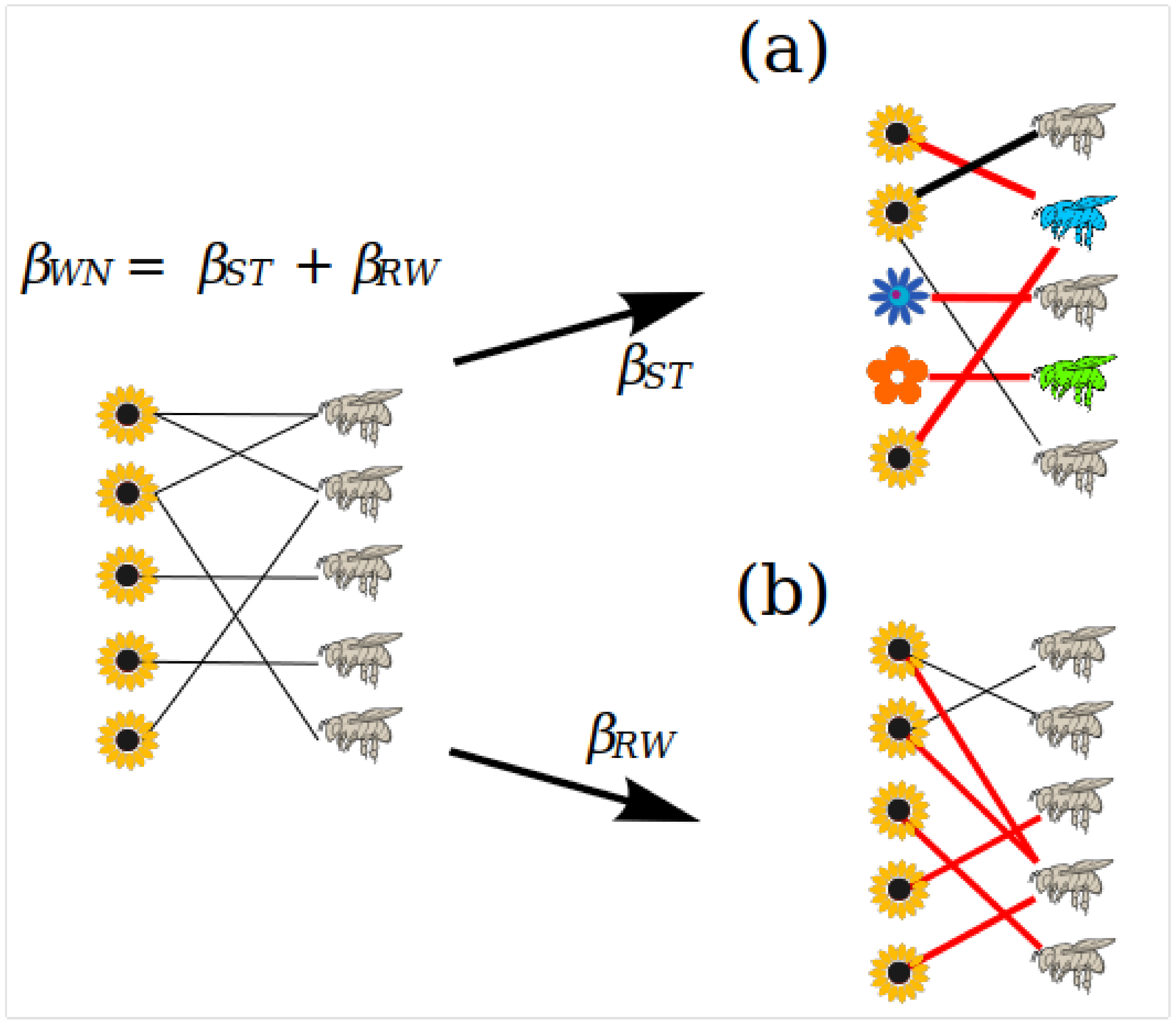
As species assemblages vary, their turnover generates variation in the way communities interact, but those species that are shared between habitats may also generate interaction variation via rewiring. It has therefore been proposed that the turnover of interactions (βWN) is the additive result of two components: i) the turnover of interactions generated by species turnover (βST) and ii) the turnover of interactions generated by the shared species between communities, interaction rewiring (βRW, Figure 3). Since we require a shared species and its turnover to have interaction turnover; βST and βRW are a subset of βWN; leading to the additive partition of the beta diversity of interactions: βWN = βST + βRW [29]. These measures are derived from the beta diversity βW [61], which is defined as:
where a is the number of shared species between communities, b is the number of unique species of the first community and c is the number of unique species of the second community. The index provides values between zero and one, where zero indicates completely similar species between communities and one denotes completely different species between communities. For the calculation of interaction turnover, a represents shared interactions between communities, while b and c represent the realized interactions within each community.
The framework to measure the beta diversity of interactions prompted the rise of a new area of study, which examines in depth how interactions are replaced independent of species identity, however, empirical studies related to this subject are still in their infancy, and little is known about the real dynamism of ecological networks in natural environments. Pioneer studies have already shown that the turnover of interactions can be explained by deterministic (niche-based) and stochastic factors (neutral theory; [60,62,63]). It has also been observed that the turnover of pollination and ant–plant mutualistic networks are high [60,63], yet there are clear differences between the main drivers of interaction beta diversity and its components. Because published evidence shows that across space and time the turnover of interactions is not equally explained by the rewiring of interactions or by the turnover of interactions driven by the turnover of species, there is always one component explaining more than the other. For instance, is has been shown that the turnover of interactions driven by the turnover of species increases with distance for pollination and ant–plant mutualistic networks [60,64], and thus as communities become less similar in terms of species composition their interactions will mainly vary due to species replacement. In another study, with ant–plant mutualisms, it was revealed that the main driver of interaction turnover between two neighboring communities sharing great numbers of species is interaction rewiring [58]. Another example found that the temporal turnover of pollination networks was mainly driven by interaction rewiring [63]. As these measures are computed to compare ecological networks, we have to acknowledge that the two groups or trophic levels that form the network may contribute in different ways to the turnover of interactions driven by species turnover. Following this, the question here is which trophic level is responsible for generating such variation if species turnover seems to be the main factor driving interaction turnover over space? For example, it has been observed in pollination networks that the interaction turnover driven by species turnover can be generated by plants [65], and in other cases by pollinators [64]. This indicates that the trophic level explaining the turnover of interactions over space is particular to the study area.
Examining the turnover of interactions in depth we can move towards identifying which species are actually the strongest contributors to network dissimilarity, particularly the rewiring of interactions. Thus by understanding the conditions under which the rewiring of interaction occur and its relation to the abundance of plants and pollinators could reveal how communities react to species loss or phenological mismatches. This is of evolutionary relevance, since floral visitors can be divided into cheaters (i.e., robbers and thieves of flower rewards) and effective pollinators and, therefore, the turnover of interactions (i.e., rewiring) could include the variation made by those non-effective pollinators. Hence, if we identify which species are the main drivers of interaction rewiring, we will understand how cheaters and effective interaction partners contribute to rewiring and their role in maintaining the stability and function of ecological networks, and ultimately plant fitness.
By studying and comparing ecological networks in terms of the identity of their pairwise interactions, we have learned that interactions vary more than species assemblages. Recent evidence has shown that the turnover of interactions is higher than the replacement of species, and intriguingly it seems that interaction turnover is correlated with factors that are not related to species turnover [66]. Such high dynamism in interactions is relevant in both temporal and spatial contexts, as the high turnover of interactions may allow all species to interact. For example, plant species without a pollen vector may have a chance to reproduce when a new pollinator arrives at its habitat [59]. Even across space, the fact that interactions are filtered and that species do not interact in the same way, may promote ecosystem stability, as if all species where able to interact without interaction filtering then ecological networks would behave as static entities, reducing robustness and ultimately ecosystem functioning [57]. This should be taken into account when explaining the distribution of biodiversity across ecological gradients, as there have been few studies so far that consider the dynamism of species interactions and its contribution to explaining global biodiversity.
4. Merging Species Interactions into Metawebs (γ-Diversity)
As we previously noted, local species assemblages are a subset of a regional pool of species, and congruently, ecological networks are a subset of regional pools of both species and their potential interactions [25,29]. If we compile a set of networks from a certain region, for example, 12 networks that represent the interactions between the pollinators and flowers of a mountain (from its base to its top), they can be merged into one network, a metaweb. The metaweb is a representation of the regional pool of potential interactions (i.e., gamma diversity of interactions), and the interactions of each of the merged networks can be compared and evaluated in relation to the sum of all networks together [67]. Note that a metaweb ideally represents all the potential interactions of a region, including all types of interactions, from symbiotic mutualisms to antagonisms, however, it is not possible to sample all the interactions of a region, and therefore, according to current knowledge, a metaweb represents the sum of the networks that a researcher wants to merge. For instance, one metaweb can be formed by the mutualistic networks of a particular habitat, which may include pollination, seed-dispersal and ant–plant protective mutualisms in a single metaweb, e.g., [22]. Conversely, another type of metaweb can represent all the mutualistic networks of a single type of interaction, such as the ant–plant protective mutualistic networks of the Neotropical savanna, e.g., [60]. Whatever the case, the approach to describing and measuring a metaweb, which represents the gamma level of the diversity of interactions, can be implemented in two different ways: (i) by estimating the gamma diversity of the full metaweb, for example using an index (e.g., H2 index) and (ii) by measuring how much a given local network and its properties differ from a metaweb formed by the local networks of the region. The first approach only gives us a single value that describes the interactions of a region, but the second can provide insightful information to describe the similarity of a local network with respect to the metaweb, which gives explanations of the interactions under a regional approach.
One way of comparing a local network with its metaweb and to describe the gamma diversity of interactions is by measuring the global variability between different networks [29]. Compared with beta diversity measures that only make pairwise comparisons, the metaweb approach allows multi-site comparisons of networks. To our knowledge, there is only one index that allows the multi-site comparison of networks, the β’OS index, which measures how dissimilar a local network is in relation to the pool of potential interactions [29]. This index measures the degree of dissimilarity between a local network and its metaweb, and it works as in the following examples. If we study a local network which has 10 realized interactions and compare them with the potential interactions in the metaweb which has 100 interactions, its dissimilarity is equal will be β’OS = 0, if all the interactions of the studied local network can be found in the metaweb. This means that the interactions of the studied network are highly similar compared with the other networks that form the metaweb. In another case, if the studied network has 10 realized interactions and it does not share interactions with the metaweb, the β’OS value will be 1 which means that the interactions of the studied network are disimilar to the other networks in the metaweb. The β’OS index provides one value for each network in the metaweb, ranging from 0 (perfect similarity with the metaweb) to 1 (complete dissimilarity with the metaweb), the frequencies of these values can be visualized, and the distribution describes the dissimilarities across the entire set of networks, e.g., [60,66]. For instance, as the values of β’OS can range from 0 to 1, if the mean of the distribution of β’OS is close to 0, then there is a low filtration of interactions (all the potential interactions are found in the local networks), whereas if the mean is close to 1 it indicates that interactions are locally filtered (few potential interactions are found in the local networks, [29]). Some studies have interpreted this index as a measure of the number of unique interactions in each of the local networks, however this is not true, as the β’OS index simply measures how different each network is from the whole metaweb, which includes the compared network. A real measure of unique interactions should exclude the focal network from the metaweb to measure its real uniqueness. A measure of interaction uniqueness could have theoretical and conservation applications. If we identify those regions with unique interactions it could be useful in finding an explanation of how some habitats filter unique set interactions and would provide valuable information to postulate useful policies to conserve not only rare species but also rare interactions [30]. The role of rare interactions should not be overlooked, as rare or endemic species might depend on such rare interactions for their persistence and to complete their life cycles, e.g., [68]. Indeed, overarching ecological network theory argues that rare interactions are part of the non-random structure of networks that maintains biodiversity, and that without it, ecological networks are not functional [69]. By identifying unique interactions we might be able to conserve species, and also conserve ecological functions and ecosystem stability [30].
5. A New Approach to Studying Biodiversity Uniqueness
One way to determine the degree of importance of the interactions of a habitat, or in a certain period of time, could be by identifying the unique and common interactions in large spatial or temporal scales. For example, if we sum the interaction networks of plants and their pollinators from several forest fragments of the same region, we could obtain the metaweb of that region and consequently, we can identify those rare and common interactions. In the same way, we could apply the same approach by merging the networks of plants and their pollinators of a single habitat but sampled every month of a year. It is now recognized that dominant and abundant species interact the most, assuming that their role in maintaining ecosystem functions is of more importance than those of rare species and interactions [70]. However, the majority of species are rare and are often considered specialists, thus identifying how and when rare interactions occur and contribute to ecosystem function may reveal novel aspects of community ecology, as this set species is the reason our planet is highly diverse [70]. As Daniel Janzen once said, “What escapes the eye, however, is a much more insidious kind of extinction: the extinction of ecological interactions” [71].
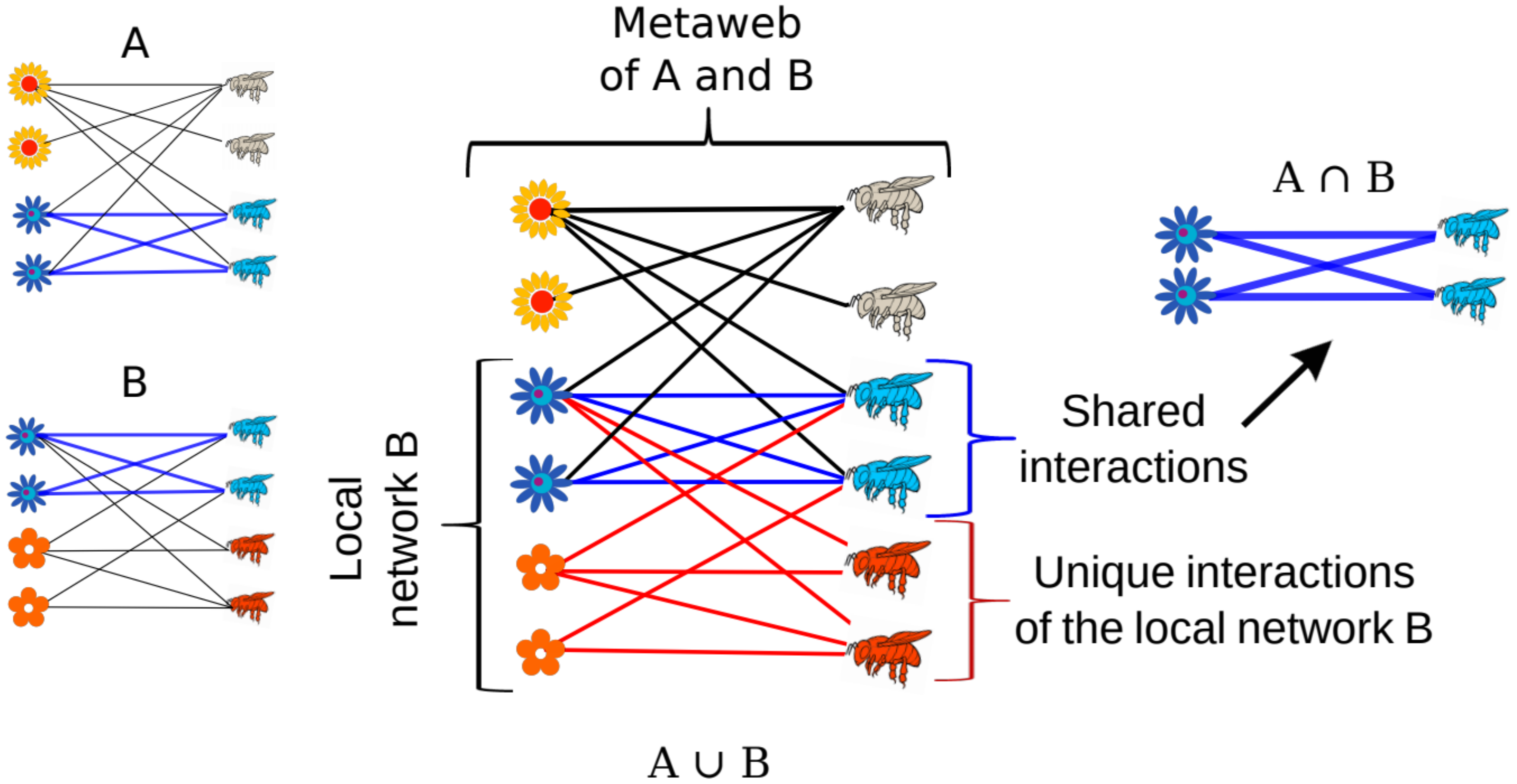
To identify the unique and common interactions we first need to acknowledge that we are working with two levels, the local (e.g., the network of a forest fragment or the network of a single month of a year; α-diversity) and the regional, which represents the sum of all the interactions sampled (e.g., the sum of the networks of all the forest fragments and all the months of the year; γ-diversity, namely, the metaweb). Each of the local networks is a piece of a greater entity, the metaweb, and thus each local network has a unique set of interacting species and therefore a unique identity. In this sense, we should be able to measure the degree of uniqueness or commonness of each of the interactions realized in each local network in relation to its metaweb, but only if the focal network is excluded from it. For instance, if the interactions of a local network are common in relation to the other interactions, this could imply that we can find the same species in all the forest fragments, establishing the same pairwise interactions. Conversely, if the local network contains a unique set of interactions, this might imply that in this forest fragment there are pairwise interactions that cannot be found in either other forest fragments or in the metaweb (Figure 4).
Here we propose two new ways to measure the uniqueness and commonness of interactions: (i) Local Network Uniqueness (LNU), which measures the proportion of unique interactions of a focal network in relation to its metaweb and (ii) Shared Interactions Frequency (SIF), which measures the proportion of common interactions of a focal network in relation to its metaweb. To calculate the LNU and SIF indexes of each network, we initially need to build a metaweb of potential interactions Mij where i represents the localities or time intervals and j represents the pairs of interactions between the observed species. We then need to build for each local network Lxj a quasimetaweb (qMij, which is simply our Mij metaweb without our network of interest Lxj, then the quasimetaweb is: qMij = Mij – Lxj. Then, the LNU and SIF of a local network L can be calculated as the following:
and
where is the mean of the occurrences of the shared interactions of a focal network with its quasimetaweb (qMij) and N is the total number of networks comprising the metaweb (Mij). The LNU index ranges from 0 (none of the interactions are unique) to 1 (all of the interactions are unique). SIF ranges from 0 (no shared interactions) to 1 (the maximum value represents that all the shared interactions are the same across all the metaweb) where N is the maximum number of local networks we are studying (Figure 5).
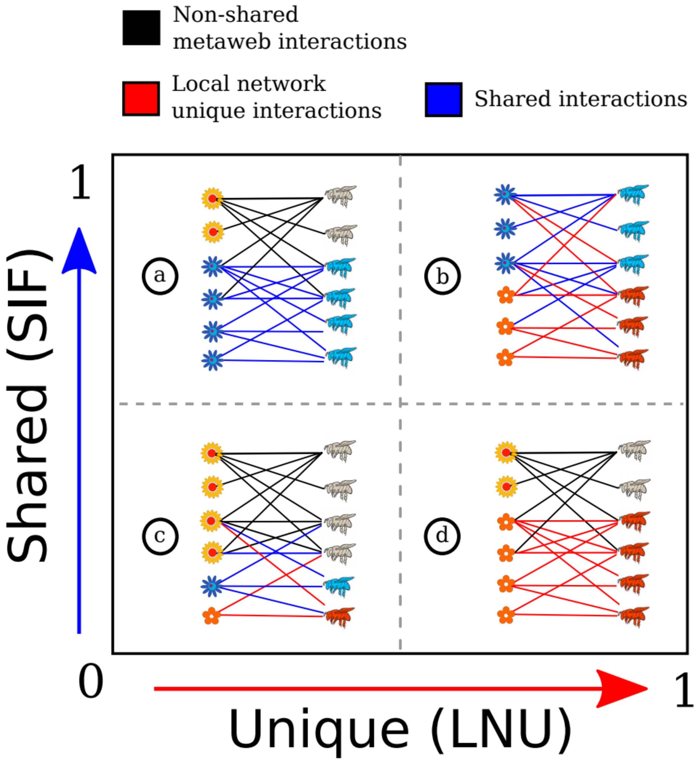
Following the logic of the LNU and SIF approaches, we can identify those networks of relevance inside a metaweb if they present many unique interactions and if the shared interactions of the local network are rare (Figure 5). In other words, the framework proposed here attempts to unravel some parameters of a metaweb: (i) how unique the shared interactions are, and how these interactions are unique in a region and it allows researchers and policymakers to determine focal areas and/or time intervals for their interests, or conservation or ecological purposes (R code is available in Supplemental Material, Code S1).
6. Concluding Remarks and the Challenge Ahead
New methods to analyze ecological networks have emerged from recognizing ecological interactions as a component of biodiversity, and now we can measure and explain how the diversity of ecological interactions varies over space and time [25]. This has allowed ecologists to go further in understanding the role of interactions for ecosystem functioning, as this approach complements traditional studies that only consider species without taking their interactions into account [3]. This because without interactions, species would not be able to reproduce (e.g., pollination), move (e.g., seed dispersal), or even coexist, as classical network studies have found that hierarchical structural properties reduce competition and promote coexistence.
In recent decades we have recognized that species loss is only a part of the most important concerns related to conservation issues [12,30]. Although species loss has become a very alarming situation, the extinction of one species also represents the extinction of its interactions which is the process that directly provides fundamental ecosystem services, and this deserves attention [72]. Indeed, future research must focus on finding and explaining the relationship between species, functional and interaction diversity, as we still do not know whether most specious regions also involve higher functional and interaction diversity. Our study is an effort to further understand an unknown component of biodiversity: species interactions. Conversely, the approach to measuring the diversity of interactions that we present in this work applies for the study of bipartite networks, thereby the extension of this approach to measure the diversity in interactions in multitrophic food webs remains an open area of research, and this topic remains to be elucidated in detail (but see [46]). In short, we have highlighted the different and newest approaches to studying species interactions and the biodiversity–ecosystem function relationship by measuring the diversity of interactions over space, time or both together.
Supplementary Materials
The following are available online at https://www.mdpi.com/1424-2818/12/3/86/s1, Code S1: R functions to measure Local Network Uniqueness (LNU) and Shared Interactions Frequency (SIF) indexes.
Author Contributions
Conceptualization, P.L., E.J.C., R.A. and W.D.; methodology, P.L., E.J.C., R.A. and W.D.; software, P.L., E.J.C., and W.D.; investigation, P.L. and W.D.; original draft preparation, P.L.; writing—review and editing, P.L., E.J.C, R.A. and W.D.; supervision, W.D. All authors have read and agree to the published version of the manuscript.
Funding
This research received no external funding.
Acknowledgments
P.L. would like to thank Claudia Suarez Barrios for her help and suggestions made while drafting of this manuscript. W. Dáttilo dedicates this work to Cauê Dáttilo de Faria (my first child who was born while we were writing this manuscript). P.L., E.C. and R.A. would like to thank Consejo Nacional de Ciencia y Tecnología, Mexico (CONACyT) for the scholarship provided (CVU: 771366, 700537, 771787 respectively). The authors also thank Claudia Moreno, Federico Escobar and Eduardo Pineda for encouraging the writing of this manuscript.
Conflicts of Interest
The authors declare no conflict of interest.
References
- Darwin, C.R. On the Origin of Species; Routledge: Abingdon, UK, 1859. [Google Scholar]
- Ings, T.C.; Hawes, J.E. The history of ecological networks. In Ecological Networks in the Tropics; Springer: Berlin, Germany, 2018; pp. 15–28. [Google Scholar]
- Andresen, E.; Arroyo-Rodríguez, V.; Escobar, F. Tropical Biodiversity: The importance of biotic interactions for its origin, maintenance, function, and conservation. Ecol. Netw. Trop. 2018, 2018, 1–13. [Google Scholar]
- Kutschera, U.; Niklas, K.J. Endosymbiosis, cell evolution, and speciation. Theory Biosci. 2005, 124, 1–24. [Google Scholar] [CrossRef] [PubMed]
- Grimaldi, D. The Co-radiations of pollinating insects and angiosperms in the Cretaceous. Ann. Mo. Bot. Gard. 1999, 86, 373–406. [Google Scholar] [CrossRef]
- Herrera, M.C.; Pellmyr, O. Plant Animal Interactions: An Evolutionary Approach; Blackwell Publishing: Hoboken, NJ, USA, 2002. [Google Scholar]
- Ollerton, J. Pollinator Diversity: Distribution, ecological function, and conservation. Annu. Rev. Ecol. Evol. Syst. 2017, 48, 353–376. [Google Scholar] [CrossRef] [Green Version]
- Escribano-Avila, G.; Lara-Romero, C.; Heleno, R.; Traveset, A. Tropical seed dispersal networks: Emerging patterns, biases, and keystone Species Traits. Ecol. Netw. Trop. 2018, 2018, 93–110. [Google Scholar]
- Falcão, J.C.F.; Dáttilo, W.; Díaz-Castelazo, C.; Rico-Gray, V. Assessing the impacts of tramp and invasive species on the structure and dynamic of ant-plant interaction networks. Biol. Conserv. 2017, 209, 517–523. [Google Scholar] [CrossRef]
- Corro, E.J.; Ahuatzin, D.A.; Jaimes, A.A.; Favila, M.E.; Ribeiro, M.C.; López-Acosta, J.C.; Dáttilo, W. Forest cover and landscape heterogeneity shape ant–plant co-occurrence networks in human-dominated tropical rainforests. Landsc. Ecol. 2019, 34, 93–104. [Google Scholar] [CrossRef]
- Inouye, D.W. Effects of climate change on alpine plants and their pollinators. Ann. N. Y. Acad. Sci. 2019, 1–12. [Google Scholar] [CrossRef]
- Valiente-Banuet, A.; Aizen, M.A.; Alcántara, J.M.; Arroyo, J.; Cocucci, A.; Galetti, M.; García, M.B.; García, D.; Gómez, J.M.; Jordano, P.; et al. Beyond species loss: The extinction of ecological interactions in a changing world. Funct. Ecol. 2015, 29, 299–307. [Google Scholar] [CrossRef]
- Galetti, M.; Guevara, R.; Côrtes, M.C.; Fadini, R.; Matter, S.V.; Leite, A.B.; Labecca, F.; Ribeiro, T.; Carvalho, C.S.; Collevatti, R.G.; et al. Functional extinction of birds drives rapid evolutionary changes in seed size. Science 2013, 340, 1086–1091. [Google Scholar] [CrossRef] [Green Version]
- Medeiros, L.P.; Garcia, G.; Thompson, J.N.; Guimarães, P.R. The geographic mosaic of coevolution in mutualistic networks. Proc. Natl. Acad. Sci. USA 2018, 115, 12017–12022. [Google Scholar] [CrossRef] [PubMed] [Green Version]
- Herrera, C.M. Variation in mutualisms: The spatio- temporal mosaic. Biol. J. Linn. Sociely 1988, 35, 95–125. [Google Scholar] [CrossRef]
- Sahley, C.T. Bat and hummingbird pollination of an autotetraploid columnar cactus, Weberbauerocereus weberbaueri (Cactaceae). Am. J. Bot. 1996, 83, 1329–1336. [Google Scholar] [CrossRef]
- Bascompte, J.; Jordano, P.; Melián, C.J.; Olesen, J.M. The nested assembly of plant-animal mutualistic networks. Proc. Natl. Acad. Sci. USA 2003, 100, 9383–9387. [Google Scholar] [CrossRef] [Green Version]
- Ings, T.C.; Montoya, J.M.; Bascompte, J.; Blüthgen, N.; Brown, L.; Dormann, C.F.; Edwards, F.; Figueroa, D.; Jacob, U.; Jones, J.I.; et al. Ecological networks—Beyond food webs. J. Anim. Ecol. 2009, 78, 253–269. [Google Scholar] [CrossRef]
- Miranda, P.N.; Ribeiro, J.E.L.D.S.; Luna, P.; Brasil, I.; Delabie, J.H.C.; Dáttilo, W. The dilemma of binary or weighted data in interaction networks. Ecol. Complex 2019, 38, 1–10. [Google Scholar] [CrossRef]
- Verdu, M.; Valiente-Banuet, A. The nested assembly of plant facilitation networks. Am. Nat. 2008, 172, 751–760. [Google Scholar] [CrossRef] [Green Version]
- Dáttilo, W.; Rico-Gray, V. Ecological Networks in the Tropics; Springer: Cham, Switzerland, 2018; ISBN 978-3-319-68227-3. [Google Scholar]
- Dáttilo, W.; Lara-Rodríguez, N.; Guimarães, P.R.; Jordano, P.; Thompson, J.N.; Marquis, R.J.; Medeiros, L.P.; Ortiz-Pulido, R.; Marcos-García, M.A.; Rico-Gray, V. Unravelling Darwin’s entangled bank: Architecture and robustness of mutualistic networks with multiple interaction types. Proc. R. Soc. Biol. 2016, 283, 1–9. [Google Scholar] [CrossRef] [Green Version]
- Dormann, C.F.; Fründ, J.; Schaefer, H.M. Identifying Causes of Patterns in Ecological Networks: Opportunities and Limitations. Annu. Rev. Ecol. Evol. Syst. 2017, 48. [Google Scholar] [CrossRef] [Green Version]
- Tylianakis, J.M.; Morris, R.J. Ecological Networks across Environmental Gradients. Annu. Rev. Ecol. Evol. Syst. 2017, 48. [Google Scholar] [CrossRef]
- Poisot, T.; Stouffer, D.B.; Gravel, D. Beyond species: Why ecological interaction networks vary through space and time. Oikos 2015, 124, 243–251. [Google Scholar] [CrossRef]
- Olesen, J.M.; Jordano, P. Geographic Patterns in Plant-Pollinator Mutualistic Networks. Ecology 2002, 83, 2416. [Google Scholar]
- Ollerton, J.; Cranmer, L. Latitudinal trends in plant-pollinator interactions: Are tropical plants more specialised? Oikos 2002, 98, 340–350. [Google Scholar] [CrossRef]
- Devoto, M.; Medan, D.; Montaldo, N.H. Patterns of interaction between plants and pollinators along an environmental gradient. Oikos 2005, 109, 461–472. [Google Scholar] [CrossRef]
- Poisot, T.; Canard, E.; Mouillot, D.; Mouquet, N.; Gravel, D. The dissimilarity of species interaction networks. Ecol. Lett. 2012, 15, 1353–1361. [Google Scholar] [CrossRef]
- Tylianakis, J.M.; Laliberté, E.; Nielsen, A.; Bascompte, J. Conservation of species interaction networks. Biol. Conserv. 2010, 143, 2270–2279. [Google Scholar] [CrossRef]
- Dyer, L.A.; Walla, T.R.; Greeney, H.F.; Stireman, J.O.; Hazen, R.F. Diversity of interactions: A metric for studies of biodiversity. Biotropica 2010, 42, 281–289. [Google Scholar] [CrossRef] [Green Version]
- Brown, J.H.; Gillooly, J.F.; Allen, A.P.; Savage, V.M.; West, G.B. Toward a metabolic theory of ecology. Ecology 2004, 87, 1771–1789. [Google Scholar] [CrossRef]
- Soberón, J. Grinnellian and Eltonian niches and geographic distributions of species. Ecol. Lett. 2007, 10, 1115–1123. [Google Scholar] [CrossRef]
- Soberón, J.; Nakamura, M. Niches and distributional areas: Concepts, methods, and assumptions. Proc. Natl. Acad. Sci. USA 2009, 106, 19644–19650. [Google Scholar] [CrossRef] [Green Version]
- Kay, K.M.; Schemske, D.W. Geographic patterns in plant-pollinator mutualistic networks: Comment. Ecology 2004, 85, 875–878. [Google Scholar] [CrossRef]
- Gotelli, N.J. Research frontiers in null model analysis. Glob. Ecol. Biogeogr. 2001, 10, 337–343. [Google Scholar] [CrossRef] [Green Version]
- Vázquez, D.P.; Bluthgen, N.; Cagnolo, L.; Chacoff, N.P. Uniting pattern and process in plant-animal mutualistic networks: A review. Ann. Bot. 2009, 103, 1445–1457. [Google Scholar] [CrossRef] [PubMed]
- Jordano, P.; Bascompte, J.; Olesen, J.M. Invariant properties in coevolutionary networks of plant-animal interactions. Ecol. Lett. 2003, 6, 69–81. [Google Scholar] [CrossRef] [Green Version]
- Hubbell, S.P. The Unified Neutral Theory of Biodiversity and Biogeography; Princeton University Press: Princeton, NJ, USA, 2001; Volume 17, ISBN 0691021295. [Google Scholar]
- Krishna, A.; Guimaraes, P.R., Jr.; Jordano, P.; Bascompte, J. A neutral-niche theory of nestedness in mutualistic networks. Oikos 2008, 117, 1609–1618. [Google Scholar] [CrossRef] [Green Version]
- Vellend, M. The Theory of Ecological Communities. Monogr. Popul. Biol. 2016, 57, 229. [Google Scholar]
- Ponisio, L.C.; Valdovinos, F.S.; Allhoff, K.T.; Gaiarsa, M.P.; Barner, A.; Guimarães, P.R.; Hembry, D.H.; Morrison, B.; Gillespie, R. A network perspective for community assembly. Front. Ecol. Evol. 2019, 7, 103. [Google Scholar] [CrossRef] [Green Version]
- Benitez-Malvido, J.; Martínez-Falcón, A.P.; Dattilo, W.; González-DiPierro, A.M.; Lombera Estrada, R.; Traveset, A. The role of sex and age in the architecture of intrapopulation howler monkey-plant networks in continuous and fragmented rain forests. Peer J. 2016, 4, e1809. [Google Scholar] [CrossRef] [Green Version]
- Ramos-Robles, M.; Dáttilo, W.; Díaz-Castelazo, C.; Andresen, E. Fruit traits and temporal abundance shape plant-frugivore interaction networks in a seasonal tropical forest. Sci. Nat. 2018, 105, 29. [Google Scholar] [CrossRef]
- Sebastián-González, E.; Dalsgaard, B.; Sandel, B.; Guimarães, P.R. Macroecological trends in nestedness and modularity of seed-dispersal networks: Human impact matters. Glob. Ecol. Biogeogr. 2015, 24, 293–303. [Google Scholar] [CrossRef]
- Bersier, L.-F.; Banasek-Richter, C.; Cattin, M.-F. Quantitative descriptors of food-web matrices. Ecology 2002, 83, 2394–2407. [Google Scholar] [CrossRef]
- Blüthgen, N.; Menzel, F.; Blüthgen, N. Measuring specialization in species interaction networks. BMC Ecol. 2006, 6, 9. [Google Scholar] [CrossRef] [PubMed] [Green Version]
- Cadotte, M.W.; Carscadden, K.; Mirotchnick, N. Beyond species: Functional diversity and the maintenance of ecological processes and services. J. Appl. Ecol. 2011, 48, 1079–1087. [Google Scholar] [CrossRef]
- Saavedra, S.; Stouffer, D.B.; Uzzi, B.; Bascompte, J. Strong contributors to network persistence are the most vulnerable to extinction. Nature 2011, 478, 233–235. [Google Scholar] [CrossRef]
- Memmott, J.; Waser, N.M.; Price, M.V. Tolerance of pollination networks to species extinctions. Proc. R. Soc. B Biol. Sci. 2004, 271, 2605–2611. [Google Scholar] [CrossRef]
- Burgos, E.; Ceva, H.; Perazzo, R.P.J.; Devoto, M.; Medan, D.; Zimmermann, M.; María Delbue, A. Why nestedness in mutualistic networks? J. Theor. Biol. 2007, 249, 307–313. [Google Scholar] [CrossRef] [Green Version]
- Benadi, G.; Hovestadt, T.; Poethke, H.J.; Blüthgen, N. Specialization and phenological synchrony of plant-pollinator interactions along an altitudinal gradient. J. Anim. Ecol. 2014, 83, 639–650. [Google Scholar] [CrossRef]
- Luna, P.; García-Chávez, J.H.; Dáttilo, W. Complex foraging ecology of the red harvester ant and its effect on soil seed bank. Acta Oecol. 2018, 86, 57–65. [Google Scholar] [CrossRef]
- Dáttilo, W. Different tolerances of symbiotic and nonsymbiotic ant-plant networks to species extinctions. Netw. Biol. 2012, 2, 127–138. [Google Scholar]
- Timóteo, S.; Ramos, J.A.; Vaughan, I.P.; Memmott, J. High Resilience of Seed Dispersal Webs Highlighted by the Experimental Removal of the Dominant Disperser. Curr. Biol. 2016, 26, 910–915. [Google Scholar] [CrossRef] [Green Version]
- Biella, P.; Akter, A.; Ollerton, J.; Tarrant, S.; Janeček, Š.; Jersáková, J.; Klecka, J. Experimental loss of generalist plants reveals alterations in plant-pollinator interactions and a constrained flexibility of foraging. Sci. Rep. 2019, 9, 1–13. [Google Scholar] [CrossRef] [PubMed] [Green Version]
- Vizentin-Bugoni, J.; Debastiani, V.J.; Bastazini, V.A.G.; Maruyama, P.K.; Sperry, J.H. Including rewiring in the estimation of the robustness of mutualistic networks. Methods Ecol. Evol. 2019, 2019, 1–11. [Google Scholar] [CrossRef] [Green Version]
- Luna, P.; Peñaloza-Arellanes, Y.; Castillo-Meza, A.L.; García-Chávez, J.H.; Dáttilo, W. Beta diversity of ant-plant interactions over day-night periods and plant physiognomies in a semiarid environment. J. Arid Environ. 2018, 156, 69–76. [Google Scholar] [CrossRef]
- Olesen, J.M.; Bascompte, J.; Elberling, H.; Jordano, P. Temporal dynamics in a pollination network. Ecology 2008, 89, 1573–1582. [Google Scholar] [CrossRef]
- Dáttilo, W.; Vasconcelos, H.L. Macroecological patterns and correlates of ant–tree interaction networks in Neotropical savannas. Glob. Ecol. Biogeogr. 2019, 2019, 1–12. [Google Scholar] [CrossRef]
- Whittaker, R.H. Vegetation of the Siskiyou Mountains, Oregon and California. Ecol. Monogr. 1960, 30, 279–338. [Google Scholar] [CrossRef]
- Burkle, L.A.; Alarcón, R. The future of plant-pollinator diversity: Understanding interaction networks acrosss time, space, and global change. Am. J. Bot. 2011, 98, 528–538. [Google Scholar] [CrossRef]
- CaraDonna, P.J.; Petry, W.K.; Brennan, R.M.; Cunningham, J.L.; Bronstein, J.L.; Waser, N.M.; Sanders, N.J. Interaction rewiring and the rapid turnover of plant-pollinator networks. Ecol. Lett. 2017, 20, 385–394. [Google Scholar] [CrossRef] [Green Version]
- Trojelsgaard, K.; Jordano, P.; Carstensen, D.W.; Olesen, J.M. Geographical variation in mutualistic networks: Similarity, turnover and partner fidelity. Proc. R. Soc. B Biol. Sci. 2015, 282, 20142925. [Google Scholar] [CrossRef] [Green Version]
- Carstensen, D.W.; Sabatino, M.; Trøjelsgaard, K.; Morellato, L.P.C. Beta diversity of plant-pollinator networks and the spatial turnover of pairwise interactions. PLoS ONE 2014, 9, e112903. [Google Scholar] [CrossRef] [Green Version]
- Poisot, T.; Cynthia, G.-J.; Fortin, M.-J.; Gravel, D.; Legendre, P. Hosts, parasites and their interactions respond to different climatic variables. Glob. Ecol. Biogeogr. 2017, 26, 942–951. [Google Scholar] [CrossRef]
- Dunne, J.A. The network structure of food webs. In Ecological Networks: Linking Structure to Dynamics in Food Webs; Oxford University Press: Oxford, UK, 2006; pp. 27–86. [Google Scholar]
- Norrbom, A.L.; Castillo-Meza, A.L.; García-Chávez, J.H.; Aluja, M.; Rull, J. A new species of Anastrepha (Diptera: Tephritidae) from Euphorbia tehuacana (Euphorbiaceae) in Mexico. Zootaxa 2014, 3780, 567–576. [Google Scholar] [CrossRef] [PubMed] [Green Version]
- Bascompte, J.; Jordano, P. Plant-Animal mutualistic networks: The architecture of biodiversity. Annu. Rev. Ecol. Evol. Syst. 2007, 38, 567–593. [Google Scholar] [CrossRef] [Green Version]
- Dee, L.E.; Cowles, J.; Isbell, F.; Pau, S.; Gaines, S.D.; Reich, P.B. When do ecosystem services depend on rare species? Trends Ecol. Evol. 2019, 34, 746–758. [Google Scholar] [CrossRef] [PubMed]
- Janzen, D.H. The deflowering of Central America. Nat. Hist. 1974, 83, 48–53. [Google Scholar]
- Chan, K.M.A.; Shaw, M.R.; Cameron, D.R.; Underwood, E.C.; Daily, G.C. Conservation planning for ecosystem services. PLoS Biol. 2006, 4, 2138–2152. [Google Scholar] [CrossRef] [Green Version]
Figure 1.
(a) Local network formed by nodes denoting five plant species (left) and five floral visitor species (right); the links represent the interactions between the species. In this bipartite network, nodes can be subdivided into two trophic levels (i.e., plants and pollinators) and interactions only occur between nodes of different trophic levels. If we count the number of different lines, we obtain the interaction richness SI. (b) Interaction matrix from which the network (a) was drawn, the numbers in the right represent the number of links per species k (i.e., degree). If we multiply the number of plant by the number of floral visitors, we obtain the network size (NZ). Each dimension of the matrix represents just one trophic level (e.g., rows = plants; columns = pollinators). (c) Hypothetical representation of the interaction of two communities (pasture and jungle), each network represents the interactions of each habitat, and the values below them describe its local properties SI, NZ and realized interactions (C). (d) Degree distribution plot of the network: we can see that we have a species with a high degree (five links) and some species with a low degree (one or two links). (e) Cumulative degree distribution following a truncated power-law.

Figure 2.
(a) A network with an equal number of links per species k (i.e., degree), which reflects a higher evenness but with high internal heterogeneity, as all species establish different numbers of interaction frequencies. (b) A network with different numbers of links per species, which reflects a lower interaction evenness but with homogeneous interaction frequencies per species. Each dimension of the matrices represents just one trophic level (e.g., rows = plants; columns = pollinators). Interaction evenness is represented by ES and interaction diversity by H2. (c) Simulated random extinction of plant species in a network, the area below the curve represents the robustness of the network (i.e., higher robustness to species extinction). (d) Simulated extinction of the most connected plant species to the least connected; the area below the curve represents the robustness of the network (i.e., lower robustness to species extinction).

Figure 3.
Conceptual diagram showing the two components of the turnover of interactions (βWN). (a) Turnover of interactions generated by the turnover of species (βST). Note that despite the turnover of species the index measures how the interaction changes between networks (red and thick lines). (b) Turnover of interaction generated by the rewiring of interactions, the same species interacting in different ways between two networks.

Figure 4.
Representation of how merging networks A and B can result in their metaweb, thus the metaweb is the union of A and B (A ∪ B). The metaweb contains the interactions of both networks and it has several characteristics that can be measured. For example, we can see that there is a subset of interaction shared between A and B (blue species and lines), this is the intersection of A and B (A ∩ B). We can also see that both A and B have a subset of unique interactions (black and red lines of the metaweb). Note that two or more networks can form a metaweb.

Figure 5.
Potential use of the Local Network Uniqueness (LNU) and Shared Interactions Frequency (SIF) indexes. Measuring the values of LNU and SIF of a set of networks, we can plot their values as the interaction uniqueness in the x-axis and commonness in the y-axis. By dividing the plot into four quadrants we can also interpret the values of LNU and SIF, in which we can have four possible scenarios denoted by the letters in the quadrants, where (a) networks with high number of shared interactions and low number of unique interactions in relation to their metaweb, (b) networks with high number of shared interactions and high number of unique interactions in relation to their metaweb, (c) networks with low number of shared interactions and low number of unique interactions in relation to their metaweb and, (d) networks with low number of shared interactions and high number of unique interactions in relation to their metaweb.

© 2020 by the authors. Licensee MDPI, Basel, Switzerland. This article is an open access article distributed under the terms and conditions of the Creative Commons Attribution (CC BY) license (http://creativecommons.org/licenses/by/4.0/).
Share and Cite
MDPI and ACS Style
Luna, P.; Corro, E.J.; Antoniazzi, R.; Dáttilo, W. Measuring and Linking the Missing Part of Biodiversity and Ecosystem Function: The Diversity of Biotic Interactions. Diversity 2020, 12, 86. https://doi.org/10.3390/d12030086
AMA Style
Luna P, Corro EJ, Antoniazzi R, Dáttilo W. Measuring and Linking the Missing Part of Biodiversity and Ecosystem Function: The Diversity of Biotic Interactions. Diversity. 2020; 12(3):86. https://doi.org/10.3390/d12030086
Chicago/Turabian StyleLuna, Pedro, Erick J. Corro, Reuber Antoniazzi, and Wesley Dáttilo. 2020. "Measuring and Linking the Missing Part of Biodiversity and Ecosystem Function: The Diversity of Biotic Interactions" Diversity 12, no. 3: 86. https://doi.org/10.3390/d12030086
Note that from the first issue of 2016, this journal uses article numbers instead of page numbers. See further details here.