Dynamics of Dislocations in Smectic A Liquid Crystals Doped with Nanoparticles

Abstract

Edge dislocations are linear defects that locally break the positional order of the layers in smectic A liquid crystals. As in usual solids, these defects play a central role for explaining the plastic properties of the smectic A phase. This work focuses on the dynamical properties of dislocations in bulk samples prepared between two glass plates and in free-standing films. The emphasis will be put on the measurement of the mobility of edge dislocations in liquid crystals either pure or doped with nanoparticles. The experimental results will be compared to the existing models.

1. Introduction

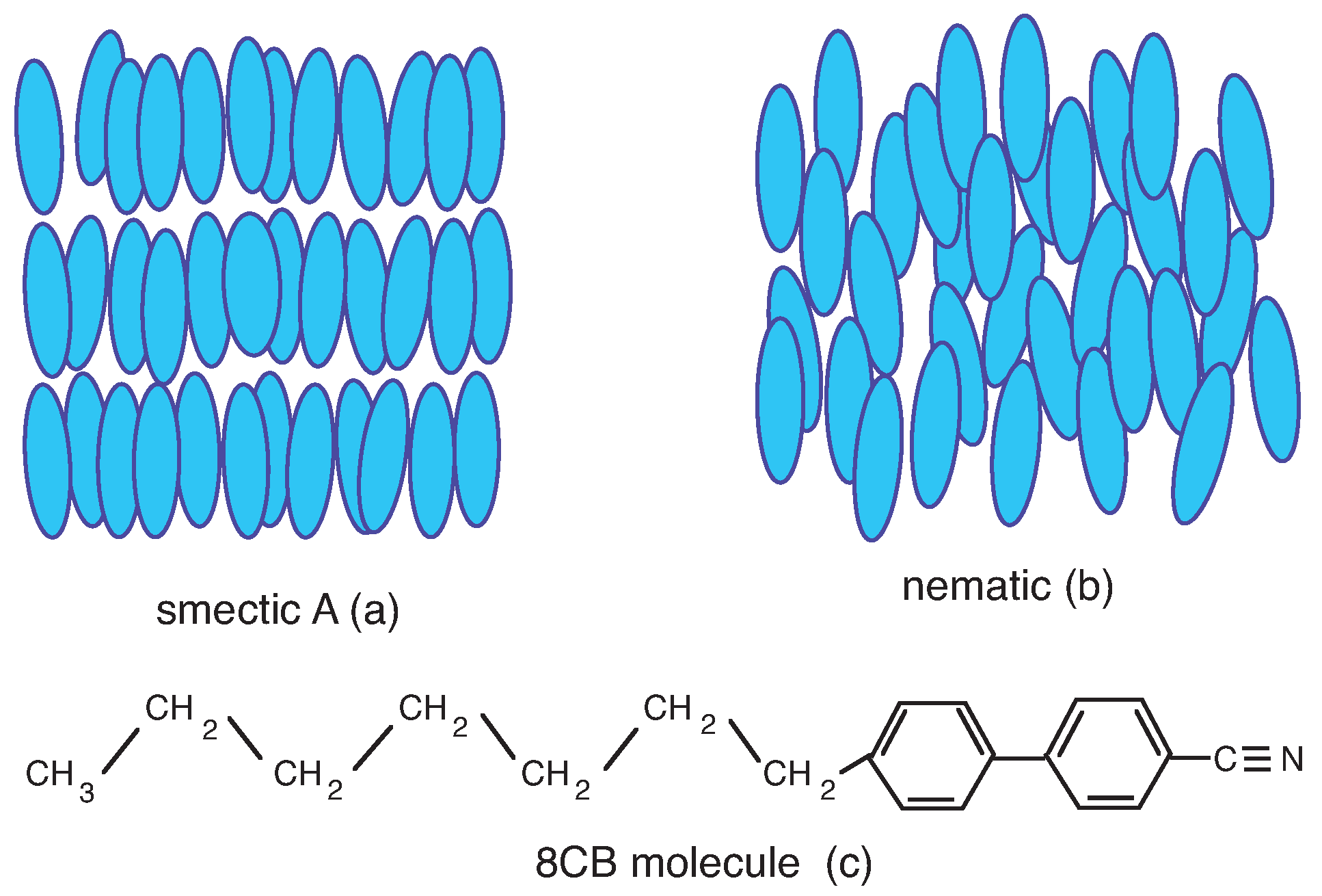
Toplogical defects are ubiquitous in all ordered systems such as crystals [1,2,3] or liquid crystals [4,5,6]. They can be punctual, linear or planar and they locally break the translational and/or rotational symmetries of the phase. In this review, I focus on dislocation dynamics in smectic A phases both in pure form and doped with nanoparticles. I recall that the smectic A phase (SmA) is a lamellar phase in which the rod-like molecules gather in fluid layers stacked on top of each other (Figure 1a). In this phase, the molecules are perpendicular to the layers on the average. This phase often transforms upon heating to a nematic phase (Figure 1b) in which only the orientational order of the molecules is conserved [7,8,9,10]. The 8CB molecule (4-n-octylcyanobiphenyl) shown in Figure 1c is a classical example of a rod-like molecule yielding a SmA and a nematic phase. All the experiments described in this paper have been performed with this liquid crystal (LC).

As in solids, the dislocations in SmA are characterized by their Burgers vector $\overrightarrow{b}$ [1,2,3]. As the layers are fluids, the only pertinent component of vector $\overrightarrow{b}$ is perpendicular to the layers [4,5,6]. In addition, b must be a multiple of the layer spacing $a_0$. There are two main types of dislocations in smectic A LC: the edge dislocations for which $\overrightarrow{b}$ is perpendicular to the dislocation line (Figure 2a) and the screw dislocations for which $\overrightarrow{b}$ is parallel to the line (Figure 2b). Although the two types of dislocations are important in plasticity, I will mainly focus on edge dislocations in this paper, with special emphasize on the measurement of their mobility, in particular when the LC is doped with nanoparticles.

The plan of the paper is as follows. In Section 1, I recall the main theoretical models developed to calculate the mobility of edge dislocations when the LC is pure (intrinsic mobility) or doped with nanoparticles. In the latter case, I show that clouds of nanoparticles, akin to Cottrell clouds in metallic alloys [1,2,11], form near the core of the dislocations and change their mobility. In Section 2, I present the experiments. I show first that the intrinsic mobility of an edge dislocation can be measured in a free-standing film. I then describe a creep experiment with homeotropic samples and I explain how to measure the intrinsic mobility of the edge dislocations when they cross screw dislocations. I show then that the mobility of the edge dislocations decrease when they drag clouds of nanoparticles, which leads to a strong hardening of the phase. In all cases, I will pay a special attention to the critical behavior of the mobility near the second-order smectic A-to-nematic phase transition.

2. Theoretical Models

I consider an edge dislocation in a smectic A monodomain. If the layers are compressed or dilated, the dislocation experiences a Peach and Koehler force of amplitude [1,2,3,9,10,12]

$$F_{PK}=\sigma b.$$

(1)

Under the action of this force, the dislocation climbs parallel to the layers with velocity v (Figure 3) and experiences a friction force of expression

$$F_v=-\frac{bv}{m_0},$$

(2)

where $b/m_0$ is a friction coefficient. In practice, the inertia of the dislocations can always be neglected so that $F_{PK}+F_v=0$. This yields $v=m_0\sigma$, where $m_0$ is defined as the intrinsic mobility of the dislocation.

2.1. Intrinsic Mobility

Two models have been proposed to calculate the mobility of an edge dislocation in a pure LC.

In the metallurgical model of Kléman and Williams [12], directly applicable to elementary edge dislocations ($b=a_0$), the mean distance l between jogs along the dislocation is of molecular size. In this case, the mobility is proportional to the self-diffusion coefficient ${\overline{D}}_{\perp }$ normal to the layers and reads, with analogy to solids:

$$m_0\approx \frac{{\overline{D}}_{\perp }{v}_{\mathrm{mol}}}{k_{B}Tl},$$

(3)

where $v_{\mathrm{mol}}$ is a molecular volume.

This model does not apply to dislocations of large Burgers vectors which are frequent in smectic A LC. This is due to the fact that, in smectics, the energy of an edge dislocation is proportional to b instead of $b^2$ as in solids [5,7,8,12,13,14,15,16,17,18]. For these dislocations, a hydrodynamic model is more appropriate [7,9,14,19,20]. Solving the hydrodynamic equations [7,9,10,21] yields:

$$m_0=A\frac{\lambda }{a_0}\sqrt{\frac{{\lambda }_p}{{\eta }_2}},$$

(4)

where A is a numerical coefficient close to 1, $\lambda =\sqrt{K/B}$ is the so-called penetration length by denoting by K (B) the bend (compression) modulus of the layers, ${\lambda }_p$ is the permeation coefficient and ${\eta }_2$ is the shear viscosity parallel to the layers [7,9,21,22]. An important result of this calculation is that the mobility is independent from the Burgers vector of the dislocation. This model also predicts a critical behavior for the mobility near the transition temperature $T_{NA}$ when the transition is second-order. It is the case in pure 8CB [23,24] where $\lambda$ diverges as $\delta T^{-\alpha }$ with $\alpha \approx 0.13$ [9] and ${\lambda }_p$ diverges as $\delta T^{-1}$ [25]. Because $a_0$ and ${\eta }_2$ do not change significantly at the transition, the hydrodynamic theory predicts that m must diverge as $\delta T^{-0.5-\alpha }$, i.e., as $\delta T^{-0.63}$ in 8CB.

2.2. Mobility in the Presence of a Cottrell Cloud

It is possible to dope a smectic A LC with gold nanoparticles of diameter $\varphi$ comparable with the layer spacing $a_0$. If the particles are correctly functionalized [26], they do not aggregate and disperse homogeneously in the smectic A phase. At the same time, they interact elastically with the edge dislocations by forming Cottrell clouds visible under the optical microscope (see the next section) [27].

As in solids [11], the volume concentration of nanoparticles around the core of the dislocation is given by a Bolzmann distribution [28]

$$c(x,z)=c_{0}exp\left(-\frac{W(x,z)}{k_{B}T}\right),$$

(5)

where $c_0$ is the concentration at infinity (equal to the average concentration in the limit of an infinite sample). In this calculation, the dislocation is located at $x=z=0$ and is parallel to the y-axis, and $W(x,z)$ is the interaction energy between the dislocation and a nanoparticle located at point $(x,z)$. The interactions between the nanoparticles are neglected. By considering that the nanoparticle behaves as a small dislocation loop of surface $\delta S$ and Burgers vector $\zeta$, Lejček calculated the interaction energy [29]:

$$W(x,z)=\delta V\frac{Bbx}{8\sqrt{\pi \lambda }}\left(\frac{exp\left(-\frac{x^2}{4\lambda \left|z\right|}\right)}{{\left|z\right|}^{3/2}}\right),$$

(6)

where $\delta V=\delta S\zeta$ is a volume change characterizing the nanoparticle.

These formulas show that the nanoparticles accumulate inside a Cottrell cloud, the limits of which are defined from the condition $\frac{W}{k_{B}T}=1$ (or, equivalently, $c/c_0=e$). By analogy, an anti-cloud forms in which the concentration is smaller than $c_0$. This anti-cloud is defined from the condition $\frac{W}{k_{B}T}=-1$ (or, equivalently, $c/c_0=1/e$). The cloud and the anti-cloud are schematically shown in Figure 4. They are composed of four elongated lobes delimited by the points of coordinates $(\pm x_{max},\pm z_1)$ and $(\pm x_1,\pm z_{max})$. It can be checked that $x_{max}\approx 1.81\sqrt{\widetilde{\delta V}}\sqrt{\lambda b}$, $z_1\approx 0.55\widetilde{\delta V}b$, $x_1\approx 1.31\sqrt{\widetilde{\delta V}}\sqrt{\lambda b}$ and $z_{max}\approx 0.86\widetilde{\delta V}b$ where $\widetilde{\delta V}=\frac{\delta V}{8\sqrt{\pi }{k}_{B}T/B}$ – of the order of unity in experiments—is the dimensionless volume change [28]. This shape is very different from the cylindrical shape of the cloud and anti-cloud found in solids. This is due to the fact the elastic stress does not propagate along the layers because of their fluidity, making the smectic A phase elastically very anisotropic.

The next question is to determine how the cloud changes the mobility of the dislocation when it climbs parallel to the layers. The answer is given by solving the diffusion equation for the concentration of nanoparticles in the reference frame $(x,y,z)$ of the moving dislocation and by then calculating the drag force on the dislocation.

The diffusion equation in the stationary regime is obtained by writing that $\mathrm{div}\overrightarrow{j}=0$ where $\overrightarrow{j}$ is the diffusion flux of nanoparticles. In a smectic A LC, this flux writes in the form:

$$\overrightarrow{j}=-\frac{c}{k_{B}T}\tilde{D}\overrightarrow{\nabla }W-\tilde{D}\overrightarrow{\nabla }c-c\overrightarrow{v},$$

(7)

with

$$\tilde{D}=\left[\begin{array}{cc}{D}_{\Vert }& 0\\ 0& D_{\perp }\end{array}\right],$$

(8)

where $D_{\Vert }$ ($D_{\perp }$) is the diffusion coefficient of the nanoparticles parallel (perpendicular) to the layers. Note that the first term in Equation (7) is the drift term due to the interaction force between the nanoparticles and the dislocation (Einstein relation), the second term is the usual anisotropic diffusion flux and the last term is the diffusion flux due to the motion of the dislocation. Writing $\mathrm{div}\overrightarrow{j}=0$ gives

$$D_{\Vert }\frac{\partial }{\partial x}\left(c\frac{\partial U}{\partial x}+\frac{\partial c}{\partial x}\right)+D_{\perp }\frac{\partial }{\partial z}\left(c\frac{\partial U}{\partial z}+\frac{\partial c}{\partial z}\right)=0,$$

(9)

where $U(x,z)=\frac{W(x,z)}{k_{B}T}+\frac{vx}{D_{\Vert }}$. This equation must be solved with the boundary condition $c=c_0$ at infinity. As for the drag force ${\overrightarrow{F}}_{\mathrm{drag}}$ exerted by the nanoparticles on the dislocation, it is given, by definition, by

$${\overrightarrow{F}}_{\mathrm{drag}}=\int \int c\overrightarrow{\nabla }Wdxdz,$$

(10)

where the integral is taken over the whole space. By using the fact that c is the solution of the diffusion equation, and by setting $\overline{c}\equiv c/c_0$, $\overline{x}\equiv x/\lambda$, $\overline{z}\equiv z/\lambda$, it can be shown that [28]

$${\overrightarrow{F}}_{\mathrm{drag}}=-\frac{k_{B}T{c}_0{\lambda }^2}{D_{\Vert }}\xi \overrightarrow{v},$$

(11)

where $\xi$ is the dimensionless drag coefficient

$$\xi =\int \int (\overline{c}-1)d\overline{x}d\overline{z}.$$

(12)

Equations (9), (11) and (12) are the basic equations of the problem.

In practice, the diffusion equation can only be solved analytically when $D_{\perp }\to 0$. In this 1D limit, the concentration field reads at velocity $v\ne 0$:

$$\left\{\begin{array}{c}c=\frac{v{c}_0}{D_{\Vert }}exp\left(-\frac{W}{k_{B}T}-\frac{vx}{D_{\Vert }}\right){\int }_{-\infty }^{x}exp\left(\frac{W}{k_{B}T}+\frac{vx}{D_{\Vert }}\right)dx\mathrm{under}\mathrm{compression}(v>0),\hfill \\ c=-\frac{v{c}_0}{D_{\Vert }}exp\left(-\frac{W}{k_{B}T}-\frac{vx}{D_{\Vert }}\right){\int }_x^{\infty }exp\left(\frac{W}{k_{B}T}+\frac{vx}{D_{\Vert }}\right)dx\mathrm{under}\mathrm{dilation}(v<0),\hfill \end{array}\right.$$

(13)

and the drag coefficient can be written under the form

$$\xi =\int \int \frac{{(\overline{c}-1)}^2}{\overline{c}}d\overline{x}d\overline{z}.$$

(14)

Note that, contrary to Equation (12), this expression is exact only in the 1D limit. This expression seems more complicated than Equation (12). I nonetheless give it because it is much easier to calculate numerically than Equation (12) due to a better convergence of the integral at infinity.

Finally, it is possible to show that, in the limit of small velocities ($\left|v\right|\ll D_{\Vert }/\varphi$) [30]

$$\xi \to {\xi }_0\approx C\left({\int }_{-{\overline{x}}_{max}}^{-\overline{b}/2}{\int }_{-{\overline{z}}_{max}}^{-\overline{b}/2}({\overline{c}}_{eq}-1)d\overline{x}d\overline{z}+{\int }_{-{\overline{x}}_{max}}^{-\overline{b}/2}{\int }_{\overline{b}/2}^{{\overline{z}}_{max}}({\overline{c}}_{eq}-1)d\overline{x}d\overline{z}\right),$$

(15)

where ${\overline{c}}_{eq}$ is the equilibrium distribution in units of $c_0$ given in Equation (5) and C is a constant equal to 2 when $D_{\perp }=0$ and of the order of 1.3 when $D_{\perp }\sim D_{\Vert }$. Note that the quantity in brackets represents the number of nanoparticles in the Cottrell cloud in units of $c_o{\lambda }^2$. This formula shows that the drag force is proportional to v and $c_0$ in the limit of small velocities (linear regime).

In practice, the diffusion equation can be solved numerically by using a finite element method (FEM). This problem is delicate because the potential $W(x,z)$ is extraordinarily “peaked” close to the core of the dislocation and diverges at the origin (Figure 5). In reality, this divergence does not exist and must be suppressed because the core of the dislocation melts. This can be shown by using a Landau–Ginzburg approach where the smectic ordering is described by a complex order parameter [31,32]. One way to avoid the divergence would be to use this formalism, but this is cumbersome. A much simpler method consists of multiplying the potential by a “core function” of the type:

$$f_c\left(r\right)={\left[arctan\left(\frac{r^2}{{(3b/2)}^2}\right)\right]}^4,$$

(16)

where $r=\sqrt{x^2+z^2}$. This function and the resulting potential $\overline{W}=W{f}_c$ are plotted in Figure 5 by taking $\delta V=28$nm${}^3$, $B={10}^7$ Pa, $\lambda =0.76$nm and $b=a_0=3$nm which are typical values for 8CB at 30 °C [9].

By using this new potential, the concentration field and the resulting drag force were numerically calculated as a function of the dislocation velocity. Two typical 3D plots of the concentration field $\overline{c}$ are shown in Figure 6 when the layers are compressed and v = 0.1 mm/s. In (a), $D_{\perp }=0$ and in (b), $D_{\perp }=D_{\Vert }$. These graphs were calculated by taking $D_{\Vert }=2\times {10}^{-12}$m${}^2$/s [30] and the same values as before for $\delta V$, B, $\lambda$ and b. They show that the Cottrell cloud deforms when the dislocation moves. In particular, the nanoparticles accumulate ahead of the dislocation, forming a bulge that is narrow in the z-direction and elongated in the x-direction (it extends over the typical distance $D_{\Vert }/v$). When $D_{\perp }=0$, this bulge is strongly pinched along the x-axis (Figure 6a). The bulge strongly flattens and its pinch-off disappears when the nanoparticles can diffuse normal to the layers (Figure 6b). By changing the velocity in the simulations, it can also be shown that both the size of the Cottrell cloud and the concentration inside decrease when the velocity increases, while the number of nanoparticles in the bulge increases and then decreases when the velocity increases, passing through a maximum for a velocity $v\approx 0.4$mm/s. This evolution shows that the cloud erodes when the velocity increases. More details about these simulations are given in Ref. [28]. We also refer to this paper for a discussion of the Cottrell cloud evolution when the layers are dilated and the dislocation moves with a negative velocity. In that case, the bulge forms on the side of the Cottrell cloud.

The drag coefficient can also be calculated as a function of velocity. The result is shown in Figure 7 where the graph has been calculated with the same values of the parameters as before. This figure shows that the friction coefficient passes through a maximum for a negative value of the velocity. This asymmetry between positive and negative velocities is due to the fact that the dislocation behavior is different under dilation and under compression. This comes from the fact that, for symmetry reasons, it is different for the dislocation to climb in the positive and negative directions of the x-axis in the presence of a Cottrell cloud. This graph also shows that $\xi$ tends to zero at very large velocity. This is due to the erosion of the Cottrell cloud. The friction coefficient also depends on the ratio $D_{\Vert }/D_{\perp }$, decreasing by a factor of ∼1.5 at small velocities ($\left|v\right|<0.1$mm/s) when this ratio passes from 0 to 1. The reader will note that the friction coefficient is not given for large negative velocities. This is not a coincidence. Indeed, these velocities are not accessible experimentally because of an undulation instability of the layers under dilation normal to the layers [33,34].

Finally, Figure 8 shows the drag coefficient as a function of the temperature difference $\delta T=T-T_{NA}$. The calculations were performed for an elementary edge dislocation propagating at 20 $\mathsf{\mu }$m/s—a typical value for velocity in the experiments with 8CB (see the next section). This graph shows that $\xi$ strongly decreases when the temperature increases and tends to 0 when $T\to T_{NA}$. This behavior is due to the critical behavior of the elastic modulus B that vanishes at $T_{NA}$.

In the next section, I describe how these predictions can be tested experimentally.

3. Experiments

Two types of samples can be used to measure the mobility of the edge dislocations: the free-standing films in which only edge dislocations are present and the homeotropic samples prepared between two glass plates in which both edge and screw dislocations are present. In films, the edge dislocations are visible under reflecting microscopy and their mobility can be obtained by directly measuring their velocity under the microscope. In homeotropic samples, the dislocations are invisible in usual conditions and the measurement of their mobility is indirect, performed with a piezoelectric rheometer by analyzing the viscoelastic response of the samples. I describe successively these two types of experiments.

3.1. Mobility Measurement in Free-Standing Films

Because of their lamellar structure, it is possible to stretch a smectic A film on a frame. Although this property was already known to Friedel at the beginning of the 20th century [35], the study of smectic films really started in the 1970s. Since that time, a considerable number of articles have been published on smectic films, including studies on phase transitions, confinement effects, thinning transitions, vibrations, hydrodynamics at 2D, etc. [9,36,37,38]. Here, I focus on the dynamics of edge dislocation loops in thick films (more than 10–20 layers, typically) and I show how the mobility of the dislocations can be deduced from these experiments.

In practice, the film is often stretched over a circular hole a few mm in diameter, drilled into a thin metallic or plastic plate. A frame of variable surface can also be used, allowing for stretching or compressing the film with a controlled velocity. The more slowly the film is stretched, the thicker it is at the end of the process. In general, the film thickness ranges between two and several hundred layers, depending on the stretching velocity. The film thickness can be precisely measured by reflectivity under a microscope. In practice, the film is related to the frame via a meniscus (Figure 9). This meniscus acts as a reservoir of matter and fixes the hydrostatic pressure P inside the film. The pressure is always lower than the atmospheric pressure $P_a$ because of the curvature of the meniscus. It can be shown that the shift of pressure $\Delta P=P_a-P$ is still given by the usual Laplace law and reads [9,39,40]:

$$\Delta P=\frac{\gamma }{\mathcal{R}}.$$

(17)

In this expression, $\gamma$ is the surface tension with air, and $\mathcal{R}$ is the radius of curvature of the meniscus which can be precisely measured by recording the intensity profile of the interference fringes observed in reflecting microscopy in the thin part of the meniscus (Figure 9).

To measure the mobility of a dislocation, a loop—hole or island—must be first nucleated. One method consists of using a deformable frame. By abruptly changing the surface area of the film, holes or islands can be nucleated, depending on whether the film is dilated or compressed [9]. As the dislocations are repulsed from the free surface in smectic A [41], the holes and the islands are dislocation loops located at mid-distance between the two free surfaces. Another more sophisticated technique to nucleate a hole is to heat the film with a tiny heating wire placed just below it. By controlling the duration and the power of the electric impulse, the film can be locally heated during a very short interval of time (1–2 ms) up to its spontaneous thinning transition temperature [9,42]. Doing that, a hole can be nucleated [39]. The film then returns in a few ms to its initial temperature fixed by the oven in which it has been stretched. With this technique, holes—which are almost always loops of elementary edge dislocation—can be nucleated. The experiment also reveals that their subsequent behavior depends on their initial radius $R_i$, the holes growing when $R_i$ is larger than some critical radius $R_c$, whereas they collapse when $R_i<R_c$. The radius $R_c$ defines the critical radius of nucleation.

This behavior can be easily understood by writing the mechanical equilibrium of the film. Indeed, the main reason for which a smectic film is stable (rigorously speaking, metastable) is due to the fact that the depression $\Delta P$ imposed by the meniscus can be balanced by the elastic stress $\sigma$ due to the elasticity of the layers. Indeed, equilibrating the normal stress at the flat surface of the film yields:

$$-P_a=-P+\sigma .$$

(18)

Note that this equation is only valid in thick films (more than 10 layers, typically) in which the disjoining pressure due to the smectic-order-induced elastic interaction between the two free surfaces (usually larger than the van der Waals force) can be neglected [42,43,44,45]. This equation shows that the layers are spontaneously compressed in films, so that each dislocation loop experiences a Peach and Koehler force of magnitude $\left|\sigma b\right|=\Delta P\left|b\right|$ which tends to make it larger when it is a hole and smaller when it is an island. To this force, add the friction force $-b\frac{v}{m}$ and the line tension force $-\frac{E}{R}$, where E is the line energy of the dislocation, R its radius and $v=\frac{dR}{dt}$. By equilibrating these three forces, one obtains by taking $b>0$ for a hole and $b<0$ for an island:

$$b\Delta P-\frac{E}{R}-b\frac{v}{m}=0.$$

(19)

This equation describes the time evolution of a loop. It shows that a loop can be at equilibrium ($v=0$) if $R=R_c=\frac{E}{b\Delta P}$, which is possible for a hole ($b>0$) but impossible for an island ($b<0$). This equilibrium is unstable since the hole collapses if its radius is smaller than $R_c$ whereas it grows if its radius is larger than $R_c$. In that case, the dislocation velocity tends to $v=m\Delta P$ when $R\gg R_c$. It must be noted that this calculation neglects the finite permeability of the meniscus [46,47], which tends to slow down the dislocation. Nevertheless, it can be shown that this effect is negligible if R is much smaller that the radius of the meniscus $R_{men}$.

These predictions were tested experimentally and used to determine the mobility m of edge dislocations in 8CB films. The first experiment was performed by using the heating wire technique. In this experiment, only holes of elementary dislocations were analyzed ($b=a_0$). It was found that, in thick films, the dislocation velocity measured at radius $R_c\ll R\ll R_{men}$ was inversely proportional to the radius of curvature $\mathcal{R}$ of the free surface of the meniscus (Figure 10), in agreement with the model. From the slope of this curve, the mobility m of an elementary edge dislocation was deduced: $m\approx 4.4\times {10}^{-8}$m${}^2$ s kg${}^{-1}$ at 28 °C. A similar experiment was performed more recently with islands obtained by compressing 8CB films with a deformable frame [48]. In this experiment, the dislocations were not elementary, but of Burgers vector $b=2a_0$ (double dislocations). In spite of this difference, the authors found a very similar value for the mobility: $m\approx 4.6\times {10}^{-8}$m${}^2$ s kg${}^{-1}$ at 27 °C. This observation confirms the predictions of the hydrodynamical model according to which the mobility is independent from b.

3.2. Mobility Measurement by Creep Test on Homeotropic Samples

Another method to measure the mobility of an edge dislocation is to study the plastic behavior of homeotropic samples. These samples are made by sandwiching the LC between two glass plates treated for homeotropic anchoring with a silane or a polyimide. With these surface treatments, the LC molecules align normal to the surfaces, resulting in smectic layers parallel to the surfaces. In plasticity, a crucial point concerns the microstructure of the samples. In usual conditions of observation, the dislocations are not visible under the microscope in homeotropic samples. They are nonetheless present, if only because the two glass plates are never perfectly parallel and always make a small angle $\alpha$. Because of this wedge geometry, an array of parallel edge dislocations, separated from each other by a distance $\mathrm{\Lambda }=b/\alpha$, forms to relax the dilatation of the layers due to the thickness variation. These “geometrical” dislocations were observed for the first time by using materials that exhibit a smectic A-to-smectic C phase transition (I recall that in the smectic C phase the molecules are tilted with respect to the normal to the layers). By approaching the phase transition temperature, the dislocations become visible between crossed polarizers, as they locally induce the tilted SmC phase [49,50] (Figure 11). This observation is crucial in plasticity because it shows that the only edge dislocations present in homeotropic samples are the geometrical dislocations. This observation was also confirmed by using a technique based on fluorescence in a lyotropic system [51]. As a consequence, it is enough to measure $\alpha$ to know the density of edge dislocations present in each sample. This is a considerable advantage with respect to solids in which the density of dislocations is very difficult to control and this makes the smectic A a perfect candidate to test models of plasticity.

In the following, I describe a piezoelectric rheometer that was specially designed to control this angle and measure the plastic response of homeotropic samples. I then recall how the plastic behavior of a homeotropic sample can be simply modeled, before explaining in which experimental conditions this simplified model can be used to measure the intrinsic mobility of edge dislocations. Finally, I report the results of mobility measurements performed in 8CB samples either pure or doped with nanoparticles, and I compare them to the theoretical predictions of the previous section before concluding.

3.2.1. Piezoelectric Rheometer

The first microplasticity experiment was conducted by Bartolino and Durand in 1977 [52]. It allowed them to measure the compression modulus of the layers B and to detect the plastic relaxation of the applied stress. In their experiment, the deformation was produced by a single piezoelectric ceramic and was extremely small (less than ${10}^{-5}$) precluding the study of defects dynamics and of their instabilities. In addition, their setup did not allow for precisely control angle $\alpha$, which is yet essential to know the density of dislocations and measure their mobility.

To remedy these shortcomings, a new rheometer was designed, allowing to both impose much larger deformations thanks to three stacks of piezoelectric ceramics and fix angle $\alpha$ with a high accuracy (to within 10${}^{-5}$ rad) thanks to three differential screws. This rheometer and its recent improvements are described in Refs. [53,54] to which we refer for a detailed description. As for the preparation of the samples, it is explained in Ref. [55].

From a mechanical point of view, the rheometer can be modeled by two springs of force constants $k_1$ and $k_2$ in series with the sample (Figure 12). In practice, the displacement $u\left(t\right)$ is imposed by three stacks of piezoelectric ceramics and the displacement $a\left(t\right)$ is measured with a linear displacement sensor. The displacements $u\left(t\right)$ and $a\left(t\right)$ and their phase shift $\mathrm{\Phi }$ are measured with a lock-in amplifier when a sinusoidal deformation is imposed to the sample. In this case, $u\left(t\right)=u_{0}sin\left(\omega t\right)$ and $a\left(t\right)=a_{0}sin(\omega t+\mathrm{\Phi })$. To fix ideas, $u_0\approx 20$nm when a sinusoidal voltage V of 1 Vrms is applied to the ceramics. The rigidity constants $k_1$ and $k_2$ can be measured with Newtonian isotropic liquids of known viscosities (silicon oils for instance).

3.2.2. Modeling the Behavior of a Homeotropic Sample

The first model of plasticity proposed to describe the behavior under compression of a homeotropic sample was proposed by the Orsay Group on Liquid Crystals [56]. In this hydrodynamical model, it was assumed that the layers could easily eliminate on the glass plates. It turns out that the predictions of this model are not at all verified experimentally. The main reason is that the layers do not eliminate on the plates as assumed in the model, certainly because of the strong anchoring of the molecules on the glass.

For this reason, a new model was proposed, based on the Orowan relation well-known in plasticity of solids [1,2]. In this metallurgical model, the deformation is attributed to the climb motion of the geometrical edge dislocations, the only ones present in the samples at equilibrium. Under this hypothesis, the motion equations read

$$\sigma =k_1(u-a)=k_2(a-\delta d),$$

(20)

$$\sigma =B\frac{\delta d}{d}-B\frac{\alpha x}{d},$$

(21)

where x is the distance covered by each dislocation at time t and d the thickness of the sample. The first equation just describes the elastic behavior of the rheometer. The second equation shows that the stress relaxes when the dislocations climb over a distance x. Knowing that $v\equiv dx/dt=m\sigma$, the elimination of x in the previous equations gives

$${\omega }_c(u-a)=(1+C)\frac{\mathrm{d}a}{\mathrm{d}t}-C\frac{\mathrm{d}u}{\mathrm{d}t},$$

(22)

where ${\omega }_c=2\pi f_c=k_{1}m\alpha$ is a stress relaxation frequency and $C=\frac{k_1}{k_2}+\frac{k_{1}d}{B}$. Solving the previous equation for a sinusoidal deformation yields

$$\left\{\begin{array}{c}\frac{a_0}{u_0}=\sqrt{\frac{{\omega }_c^2+C^2{\omega }^2}{{\omega }_c^2+{(1+C)}^2{\omega }^2}},\hfill \\ tan\left(\mathrm{\Phi }\right)=-\frac{\omega {\omega }_c}{{\omega }_c^2+C(1+C){\omega }^2}.\hfill \end{array}\right.$$

(23)

These equations show that measuring the ratio $a_0/u_0$ and the phase shift $\mathrm{\Phi }$ as a function of the frequency $\omega$ is enough to determine C and ${\omega }_c$ and then deduce the mobility m knowing $\alpha$. However, the model applies if several conditions which I enumerate below are fulfilled.

The first condition is that the elastic stress imposed to the sample must never exceed the critical stress of the undulation instability of the layers. This condition reads

$${\sigma }_{\max }<{\sigma }_c,$$

(24)

where ${\sigma }_{\max }$ is the maximum stress sustained by the sample, given by

$${\sigma }_{\max }=k_1{a}_0\sqrt{1+\frac{u_0^2}{a_0^2}-2cos\mathrm{\Phi }\frac{a_0}{u_0}}$$

(25)

and ${\sigma }_c$ the critical stress for the undulation instability, of expression [9,33]

$${\sigma }_c=2\pi \sqrt{\frac{KB}{d}}.$$

(26)

If this condition is not fulfilled, the layers break and new dislocations nucleate, which makes the sample much more ductile and unusable to determine the mobility of the edge dislocations.

The second condition is that the screw dislocations, which are always present in the samples, do not destabilize. This is the case if ${\sigma }_{\max }$ does not exceed the critical stress ${\sigma }^{\star }$ above which the screw dislocations develop an helical instability, which is equivalent of nucleating a loop of edge dislocation [9,57,58,59]. This condition reads

$${\sigma }_{\max }<{\sigma }^{\star },$$

(27)

where

$${\sigma }^{\star }=\frac{2\pi \mathcal{T}}{bd}$$

(28)

by denoting by $\mathcal{T}$ the line tension of a screw dislocation, first calculated by Bourdon et al. [57] for a helicoidal shape. It turns out that, in 8CB, ${\sigma }^{\star }>{\sigma }^c$, so that inequality (27) is less restrictive than inequality (24).

These two conditions fix the maximum value of the amplitude $u_0^{\max }$ that can be used experimentally to satisfy the basic assumption of the model, namely a constant density of edge dislocations.

The third condition to satisfy is more subtle, and comes from the fact that the moving edge dislocations inevitably cross the screw dislocations present in the samples [60,61,62,63,64,65]. These crossings are clearly visible at the smectic A-smectic C phase transition temperature because they produce transient cusps on the edge dislocations [66,67,68]. The crossings are also thermally activated with an activation energy equal to the energy $E_{\mathrm{kink}}$ of the kink formed on each edge dislocation during the crossing. By taking the crossings into account, it can be shown that the edge dislocations propagate with an effective mobility lower than their intrinsic mobility, of expression [55]

$$m_0^{\mathrm{eff}}=\frac{m_0}{1+A\frac{\sigma }{sinh(\sigma {\Omega }_a/k_{B}T)}},$$

(29)

where $A=(2bL/{\pi }^{2}E)e^{E_{\mathrm{kink}}/k_{B}T}$. In this formula, b is the Burgers vector of the edge dislocations, L is the mean distance between the screw dislocations and ${\mathsf{\Omega }}_a=Lb{a}_0$ is an activation volume calculated by assuming that the screw dislocations are elementary, which is likely as their energy is proportional to the square of their Burgers vector [69,70,71]. The ratio $m_0^{\mathrm{eff}}/m$ is plotted in Figure 13 as a function of the applied stress. This graph shows that the mobility decreases at low stress, but is equal to the intrinsic mobility under large stress.

For this reason, the simplified model fails at small applied stress. By contrast, it applies under large stress, in particular when ${\sigma }_{\max }$ is chosen just below the onset of undulation of the layers [55]. In that case, the fit of the experimental curves with the Equations (23) of the simplified model (Figure 14) directly gives the intrinsic mobility of the dislocations.

All the mobility measurements presented in the next two paragraphs have been performed under these experimental conditions by using the simplified model.

3.2.3. Dislocation Mobility in the Pure LC

The mobility of edge dislocations was systematically measured as a function of temperature in a 95 $\mu$m-thick sample with $\alpha =5\times {10}^{-4}$rad [30]. Under these experimental conditions, the dislocations are elementary. The results shown in Figure 15 show that the mobility increases with temperature and diverges at the transition temperature $T_{NA}$. The fit with relation

$$m_0=aexp\left(-\frac{E}{k_{B}T}\right)+b{(-\delta T)}^n,$$

(30)

where the first and second terms represent, respectively, a thermally activated behavior far from the transition and a critical behavior close to $T_{NA}$ (with $\delta T=T-T_{NA}<0$), gives an activation energy of 1.4 ± 0.33 eV and a critical exponent $n=-0.66\pm 0.074$. This exponent is very close to the theoretical exponent $-0.63$ given in the theoretical section. Note that three other measurements have been reported in this graph. Two of them (crosses) were obtained from a creep experiment at constant stress [73] , while the star corresponds to the measurements in free-standing films presented above [40]. A very good agreement is found between the different measurements.

The mobility of double dislocations was also measured in 8CB [55]. These dislocations spontaneously form in the samples when $\alpha ={10}^{-3}$rad to minimize their energy [9,74,75,76]. For these dislocations, it was found $m=1.2\times {10}^{-7}$m${}^2$ s kg${}^{-1}$ at ${32}^{\circ }$C ($\delta T=-1.3$ °C). This value is very close to the mobility of elementary dislocations shown in Figure 15. This measurement confirms that the mobility is independent from the Burgers vector, in agreement with the hydrodynamical model.

3.2.4. Dislocation Mobility in the LC Doped with Nanoparticles

In these experiments, the 8CB was doped with gold nanoparticles of nominal diameter 4.7 nm. Three concentrations were used: 0.1 wt %, 0.225 wt % and 0.65 wt %. To avoid the nanoparticles from aggregating, they were capped with mesogenic ligands following a procedure given in Ref. [26]. Under these conditions, the nanoparticles interact very little between them. However, they strongly interact with dislocations by forming Cottrell clouds. The latter decorate the dislocations which become visible under the microscope in natural light (Figure 16).

To measure the mobility of elementary edge dislocations, homeotropic samples of doped 8CB were prepared with an angle of $5\times {10}^{-4}$rad. Systematic measurements showed that the higher the concentration of nanoparticles, the harder the sample. This hardening is due to the drag force ${\overrightarrow{F}}_{\mathrm{drag}}$ that the Cottrell cloud exerts on the dislocation. As this force is proportional to $\overrightarrow{v}$ according to Equation (11), it adds to the viscous force ${\overrightarrow{F}}_v=-\frac{b}{m_0}\overrightarrow{v}$. As a consequence, it is as if the dislocation had a mobility m given by

$$-\frac{b\overrightarrow{v}}{m}=-\frac{b\overrightarrow{v}}{m_0}-\frac{k_{B}T{c}_0{\lambda }^2}{D_{\Vert }}\xi \overrightarrow{v},$$

(31)

where $\xi$ is the dimensionless drag coefficient given in Equation (12). In experiments, the velocity of the dislocations never exceeds $50\mathsf{\mu }$m/s. For this reason, the nonlinear effects due to the erosion of the cloud are negligible and $\xi$ is approximately constant, equal to the constant ${\xi }_0$ given in Equation (15).

In experiments, m is directly measured. Because $m_0$ is known, plotting $\frac{1}{m}-\frac{1}{m_0}$ directly gives the drag coefficient $\frac{k_{B}T{c}_0{\lambda }^2}{D_{\Vert }}{\xi }_0$ divided by b. This quantity is plotted in Figure 17 as a function of temperature for the three concentrations studied. This graph shows that the drag coefficient vanishes at $T_{NA}$ and strongly increases when the temperature decreases. It is also proportional to the concentration of nanoparticles, in agreement with the theoretical model. Finally, these curves can be fitted with the model, after remembering that $D_{\Vert }=k_{B}T/\left(4\pi {\eta }_3{\mathrm{\Phi }}_h\right)$ [19], where ${\eta }_3$ is the shear viscosity in the plane of the layers measured by Schneider in 8CB [77] and ${\mathrm{\Phi }}_h$ the hydrodynamical diameter of the nanoparticles with the ligands attached to their surface, of the order of $2\mathrm{\Phi }$. The best fit of the experimental data (solid lines in Figure 17) gives $\delta V\approx 29$nm${}^3$. This value is close to the expected theoretical value: $\delta V$(theo) = 27 nm${}^3$ obtained by taking $\delta S=\pi {\mathrm{\Phi }}^2/4=17$nm${}^2$ and $\zeta =\mathrm{\Phi }-a_0=1.6$nm (by assuming that the ligands do not deform the layers). From these data, the number of nanoparticles in the Cottrell cloud per unit length of dislocation can also be estimated [30]. For instance, this number varies from $\sim 0$ at the transition temperature $T_{NA}$ to $\sim 2\times {10}^7$m${}^{-1}$ at $\delta T=-{10}^{\circ }$C for a concentration of nanoparticles of 0.225% by weight.

4. Conclusions and Outlooks

These studies show that smectic liquid crystals are unique materials to study dislocations dynamics and test models of plasticity. Their main advantage over solids is that their microstructure can be finely controlled. This is particularly the case in homeotropic samples in which the density and the Burgers vector of the edge dislocations can be chosen just by changing the angle between the plates. Thanks to this, the hydrodynamical model for the mobility of the edge dislocations has been validated as well as the model of plasticity by climb of edge dislocations controlled by the crossings with screw dislocations. Several instabilities predicted by the theory have also been observed experimentally. I am referring here to the undulation instability of the layers and to the sequence of helical instabilities of the screw dislocations which I mentioned a number of times in this paper. Finally, the experiments with nanoparticles allowed to provide evidence of a strong hardening of the homeotropic samples that was explained in terms of drag force due to the Cottrell clouds attached to the dislocations. On this topic, I emphasize that the observed hardening could help to improve the lubrication performance of the smectic A phase [78,79].

In the future, it would be interesting to test this point. Another theoretical prediction not yet implemented experimentally concerns the nonlinear behavior of the drag force acting on edge dislocations at large velocities in the presence of Cottrell clouds. Indeed, the theory predicts that the dimensionless drag coefficient $\xi$ must decrease by a factor of 2 when the dislocation velocity passes from 0 to 0.3 mm/s, typically. This variation could be detected experimentally by performing a stress relaxation experiment under compression (to avoid the undulation instability) of very thin homeotropic samples (to avoid the helical instabilities of the screw dislocations). In these experimental conditions, the relaxation should no longer be exponential as usually observed under small stress conditions [9,80]. It would also be interesting to perform similar experiments with other materials than 8CB, in particular close to the smectic A–smectic C phase transition where the pinning between edge and screw dislocations seems more important than in 8CB for reasons that are not clear. Finally, I mention the existence of a few measurements of the mobility of edge dislocations in lamellar lyotropic phases. In these materials, the values found can vary from ∼${10}^{-7}$ m${}^2$ s kg${}^{-1}$ in the C${}_{12}$E${}_5$-H${}_2$O system [81] or the SDS-1pentanol-H${}_2$O system [82] down to ${10}^{-17}$m${}^2$ s kg${}^{-1}$ in a phospholipidic lamellar phase [51]. These differences could be due to the existence or not of microscopic defects inside the lamellae such pores or passages which favor the permeation [83,84,85,86,87,88].

References

- Friedel, J. Dislocations; Pergamon Press: Oxford, UK, 1964. [Google Scholar]
- Nabarro, F.R.N. Theory of Crystal Dislocations; Dover: New York, NY, USA, 1987. [Google Scholar]
- Landau, L.; Lifshitz, E. Theory of Elasticity, Second Edition; Pergamon Press: New York, NY, USA, 1981. [Google Scholar]
- Kléman, M. Points, Lines and Walls: In Liquid Crystals, Magnetic Systems and Various Ordered Media; John Wiley & Sons Inc.: Hoboken, NJ, USA, 1982. [Google Scholar]
- Kléman, M. Defects in liquid crystals. Rep. Prog. Phys. 1989, 52, 555–654. [Google Scholar] [CrossRef]
- Kléman, M.; Friedel, J. Disclinations, dislocations, and continuous defects: A reappraisal. Rev. Mod. Phys. 2008, 80, 61–115. [Google Scholar] [CrossRef] [Green Version]
- De Gennes, P.G.; Prost, J. The Physics of Liquid Crystals; Pergamon Press: Oxford, UK, 1995. [Google Scholar]
- Oswald, P.; Pieranski, P. Nematic and Cholesteric Liquids Crystals: Concepts and Physical Properties Illustrated by Experiments; Taylor & Francis: Boca Raton, FL, USA, 2005. [Google Scholar]
- Oswald, P.; Pieranski, P. Smectic and Columnar Liquids Crystals: Concepts and Physical Properties Illustrated by Experiments; Taylor & Francis: Boca Raton, FL, USA, 2006. [Google Scholar]
- Oswald, P. Rheophysics The Deformation and Flow of Matter; Cambridge University Press: Cambridge, UK, 2009. [Google Scholar]
- Hirth, J.P.; Lothe, J. Theory of Dislocations, 2nd ed.; Clarendon Press: Oxford, UK, 1992. [Google Scholar]
- Kléman, M.; Williams, C. Interaction between parallel edge dislocation lines in a smectic A liquid crystal. J. Phys. Lett. (France) 1974, 35, L49–L51. [Google Scholar] [CrossRef]
- Kléman, M. Linear theory of dislocations in a smectic A. J. Phys. (France) 1974, 35, 595–600. [Google Scholar] [CrossRef]
- Holyst, R.; Oswald, P. Dislocations in uniaxial lamellar phases of liquid crystals, polymers and amphiphilic systems. Int. J. Mod. Phys. B 1995, 9, 1515–1573. [Google Scholar] [CrossRef]
- Géminard, J.C.; Laroche, C.; Oswald, P. Edge dislocation in a vertical smectic-A film: Line tension versus film thickness and Burgers vector. Phys. Rev. E 1998, 58, 5923–5925. [Google Scholar] [CrossRef]
- Brener, E.A.; Marchenko, V.I. Nonlinear theory of dislocations in smectic crystals: An exact solution. Phys. Rev. E 1999, 59, R4752–R4753. [Google Scholar] [CrossRef] [PubMed] [Green Version]
- Santangelo, C.D.; Kamien, R.D. Bogomol’nyi, Prasad, and Sommerfield Configurations in Smectics. Phys. Rev. Lett. 2003, 91, 045506. [Google Scholar] [CrossRef]
- Santangelo, C.D.; Kamien, R.D. Curvature and topology in smectic-A liquid crystals. Proc. R. Soc. A 2005, 461, 2911–2921. [Google Scholar] [CrossRef] [Green Version]
- De Gennes, P.G. Viscous flow in smectic A liquid crystals. Phys. Fluids 1974, 17, 1645–1654. [Google Scholar] [CrossRef]
- Dubois-Violette, E.; Guazzelli, E.; Prost, J. Dislocation motion in layered structures. Phil. Mag. 1983, 48, 727–747. [Google Scholar] [CrossRef]
- Martin, P.C.; Parodi, O.; Pershan, P.S. Unified Hydrodynamic Theory for Crystals, Liquid Crystals, and Normal Fluids. Phys. Rev. A 1972, 6, 2401–2420. [Google Scholar] [CrossRef] [Green Version]
- Oswald, P. Lien entre perméation et dislocations vis dans les phases lamellaires. C. R. Acad. Sci. Sér. II 1987, 304, 1043–1046. [Google Scholar]
- Denolf, K.; Van Roie, B.; Glorieux, C.; Thoen, J. Effect of Nonmesogenic Impurities on the Order of the Nematic to Smectic-A Phase Transition in Liquid Crystals. Phys. Rev. Lett. 2006, 97, 107801. [Google Scholar] [CrossRef] [PubMed]
- Çetinkaya, M.C.; Yildiz, S.; Özbek, H.; Losada-Pérez, P.; Leys, J.; Thoen, J. High-resolution birefringence investigation of octylcyanobiphenyl (8CB): An upper bound on the discontinuity at the smectic-A to nematic phase transition. Phys. Rev. E 2013, 88, 042502. [Google Scholar] [CrossRef] [PubMed]
- Brochard, F. Dynamique des fluctuations près d’une transition smectique A-nématique du 2e ordre. J. Phys. (France) 1973, 34, 411–422. [Google Scholar] [CrossRef]
- Milette, J.; Toader, V.; Reven, L.; Lennox, R.B. Tuning the miscibility of gold nanoparticles dispersed in liquid crystals via the thiol-for-DMAP reaction. J. Mater. Chem. 2011, 21, 9043–9050. [Google Scholar] [CrossRef]
- Milette, J.; Relaix, S.; Lavigne, C.; Toader, V.; Cowling, S.J.; Saez, I.M.; Lennox, R.B.; Goodby, J.W.; Reven, L. Reversible long-range patterning of gold nanoparticles by smectic liquid crystals. Soft Matter 2012, 8, 6593–6598. [Google Scholar] [CrossRef]
- Oswald, P.; Lejček, L. Drag of a Cottrell atmosphere by an edge dislocation in a smectic-A liquid crystal. Eur. Phys. J. E 2017, 40, 84. [Google Scholar] [CrossRef]
- Lejček, L. Point-like impurity-dislocation interactions in smectic A liquid crystals. Liq. Cryst. 1986, 1, 473–482. [Google Scholar] [CrossRef]
- Oswald, P.; Milette, J.; Relaix, S.; Reven, L.; Dequidt, A.; Lejček, L. Alloy hardening of a smectic A liquid crystal doped with gold nanoparticles. EPL 2013, 103, 46004. [Google Scholar] [CrossRef]
- Slavinec, M.; Kralj, S.; Žumer, S.; Sluckin, T.J. Surface depinning of smectic-A edge dislocations. Phys. Rev. E 2001, 63, 031705. [Google Scholar] [CrossRef] [PubMed]
- Ambrožič, M.; Kralj, S.; Žumer, S.; Svenšek, D. Annihilation of edge dislocations in smectic-A liquid crystals. Phys. Rev. E 2004, 70, 051704. [Google Scholar] [CrossRef] [PubMed]
- Ribotta, R.; Durand, G. Mechanical instabilities of smectic-A liquid crystals under dilative or compressive stresses. J. Phys. (France) 1977, 38, 179–204. [Google Scholar] [CrossRef]
- Clark, N.; Hurd, A.J. Elastic light scattering by smectic A focal conic defects. J. Phys. (France) 1982, 43, 1159–1165. [Google Scholar] [CrossRef] [Green Version]
- Friedel, G. Mesomorphic states of matter. Ann. Phys. (Paris) 1922, 18, 273–474. [Google Scholar]
- Pershan, P.S. Structure of Liquid Crystal Phases; World Scientific: Singapore, 1988. [Google Scholar]
- De Jeu, W.H.; Ostrovskii, B.I.; Shalaginov, A.N. Structure and fluctuations of smectic membranes. Rev. Mod. Phys. 2003, 75, 181–235. [Google Scholar] [CrossRef] [Green Version]
- Stannarius, R.; Harth, K. Inclusions in freely suspended smectic films. In Liquid Crystals with Nano and Microparticles; Word Scientific: Singapore, 2016. [Google Scholar]
- Géminard, J.C.; Holyst, R.; Oswald, P. Meniscus and Dislocations in Free-Standing Films of Smectic-A Liquid Crystals. Phys. Rev. Lett. 1997, 78, 1924–1928. [Google Scholar] [CrossRef]
- Picano, F.; Holyst, R.; Oswald, P. Coupling between meniscus and smectic-A films: Circular and catenoid profiles, induced stress, and dislocation dynamics. Phys. Rev. E 2000, 62, 3747–3757. [Google Scholar] [CrossRef]
- Lejček, L.; Oswald, P. Influence of surface tension on the stability of edge dislocations in smectic A liquid crystals. J. Phys. II (France) 1991, 1, 931–937. [Google Scholar] [CrossRef]
- Picano, F.; Oswald, P.; Kats, E. Disjoining pressure and thinning transitions in smectic-A liquid crystal films. Phys. Rev. E 2001, 63, 021705. [Google Scholar] [CrossRef] [PubMed]
- Poniewierski, A.; Oswald, P.; Holyst, R. Contact Angle between Smectic Film and Its Meniscus. Langmuir 2002, 18, 1511–1517. [Google Scholar] [CrossRef]
- Jacquet, R.; Schneider, F. Dependence of film tension on the thickness of smectic films. Phys. Rev. E 2003, 67, 021707. [Google Scholar] [CrossRef] [PubMed]
- Dolganov, P.V.; Cluzeau, P.; Joly, G.; Dolganov, V.K.; Nguyen, H.T. Interaction of surfaces in smectic membranes and their instability near thinning transitions. Phys. Rev. E 2005, 72, 031713. [Google Scholar] [CrossRef] [PubMed]
- Oswald, P.; Pieranski, P.; Picano, F.; Holyst, R. When Boundaries Dominate: Dislocation Dynamics in Smectic Films. Phys. Rev. Lett. 2001, 88, 015503. [Google Scholar] [CrossRef] [PubMed] [Green Version]
- Caillier, F.; Oswald, P. Direct measurement of the permeability of the meniscus bordering a free-standing smectic-A film. Phys. Rev. E 2004, 70, 031704. [Google Scholar] [CrossRef]
- Dolganov, P.V.; Kats, E.I.; Joly, G.; Dolganov, V.K. Collapse of Islands in Freely Suspended Smectic Nanofilms. JETP Lett. 2017, 106, 229–233. [Google Scholar] [CrossRef]
- Meyer, R.B.; Stebler, B.; Lagerwall, S.T. Observation of edge dislocations in smectic liquid crystals. Phys. Rev. Lett. 1978, 41, 1393–1397. [Google Scholar] [CrossRef]
- Lagerwall, S.T.; Meyer, R.B.; Stebler, B. Direct observation of dislocations in smectics. Ann. Phys. (Paris) 1978, 3, 249–255. [Google Scholar] [CrossRef]
- Chan, W.K.; Webb, W.W. Observation of elementary edge dislocations in phospholipid multilayers and of their annealing as a determination of the permeation coefficient. J. Phys. (France) 1981, 42, 1007–1013. [Google Scholar] [CrossRef]
- Bartolino, R.; Durand, G. Plasticity in a Smectic-A Liquid Crystal. Phys. Rev. Lett. 1977, 39, 1346–1349. [Google Scholar] [CrossRef]
- Oswald, P.; Le Fur, D. Réalisation d’une cellule de déformation adaptée à l’étude des cristaux liquides smectiques. C. R. Acad. Sci. (Paris) Sér. II 1981, 297, 699. [Google Scholar]
- Oswald, P. Viscoelasticity of a homeotropic nematic slab. Phys. Rev. E 2005, 92, 062508. [Google Scholar] [CrossRef]
- Oswald, P.; Poy, G. Dislocations dynamics during the nonlinear creep of a homeotropic sample of smectic-A liquid crystal. Eur. Phys. J. E 2018, 41, 73. [Google Scholar] [CrossRef]
- Orsay Group on Liquid Crystals. On some flow properties of smectic A. J. Phys. Colloq. (France) 1975, 36, C1-305–C1-313. [Google Scholar]
- Bourdon, L.; Kléman, M.; Lejček, L.; Taupin, D. On static helical instabilities of screw dislocations in a SmA phase and on their consequence on plasticity. J. Phys. (France) 1981, 42, 261–268. [Google Scholar] [CrossRef] [Green Version]
- Oswald, P.; Kléman, M. Experimental evidence for helical instability of screw dislocation lines in a smectic A phase. J. Phys. Lett. (France) 1981, 45, L319–L328. [Google Scholar] [CrossRef]
- Herke, R.A.; Clark, N.A.; Handschy, M.A. Dynamic behavior of oscillatory plastic flow in a smectic liquid crystal. Phys. Rev. E 1997, 56, 3028. [Google Scholar] [CrossRef]
- Ishikawa, K.; Uemera, T.; Takezoe, H.; Fukuda, A. Screw dislocations decorated by disclinations of C-directors observed in thin ferroelectric smectic liquid crystal cells. Jpn. J. Appl. phys. 1984, 23, L666–L669. [Google Scholar] [CrossRef]
- Kléman, M.; Williams, C.E.; Costello, J.M.; Gulik-Krzywicki, T. Defect structures in lyotropic smectic phases revealed by freeze-fracture electron microscopy. Philos. Mag. 1977, 35, 33–56. [Google Scholar] [CrossRef]
- Allain, M. Possible defect-mediated phase transition in a lyotropic liquid crystal. Electron microscopy observations. Europhys. Lett. 1986, 2, 597–602. [Google Scholar] [CrossRef]
- Zasadzinski, J.A.N. Direct observations of dislocations in thermotropic smectics using freeze-fracture replication. J. Phys. (France) 1990, 51, 747–756. [Google Scholar] [CrossRef]
- Lelidis, I.; Blanc, C.; Kléman, M. Optical and confocal microscopy observations of screw dislocations in smectic-A liquid crystals. Phys. Rev. E 2006, 74, 051710. [Google Scholar] [CrossRef]
- Repula, A.; Grelet, E. Elementary Edge and Screw Dislocations Visualized at the Lattice Periodicity Level in the Smectic Phase of Colloidal Rods. Phys. Rev. Lett. 2018, 121, 097801. [Google Scholar] [CrossRef] [Green Version]
- Lelidis, I.; Kléman, M.; Martin, J.L. Dislocation Mobility in Smectic Liquid Crystals. Mol. Cryst. Liq. Cryst. Sci. Technol. Sect. A 1999, 330, 457–464. [Google Scholar] [CrossRef]
- Lelidis, I.; Kléman, M.; Martin, J.L. Static and dynamic observations of dislocations and other defects in smectic Cano wedges. Mol. Cryst. Liq. Cryst. Sci. Technol. Sect. A 2000, 351, 187–196. [Google Scholar] [CrossRef]
- Blanc, C.; Zuodar, N.; Lelidis, I.; Kléman, M.; Martin, J.L. Defect dynamics in a smectic Grandjean-Cano wedge. Phys. Rev. E 2004, 69, 011705. [Google Scholar] [CrossRef]
- Kléman, M. Dislocations vis et surfaces minima dans les smectiques A. Phil. Mag. 1976, 34, 79–87. [Google Scholar] [CrossRef]
- PLeiner, H. Energetics of screw dislocations in smectic A liquid crystals. Liq. Cryst. 1988, 3, 249–258. [Google Scholar] [CrossRef]
- Tian-You, F.; Xian-Fang, L. The stress field and energy of screw dislocation in smectic A liquid crystals and the mistakes of the classical solution. Chin. Phys. J. 2014, 23, 046102. [Google Scholar]
- Żywociński, A.; Picano, F.; Oswald, P.; Géminard, J.C. Edge dislocation in a vertical smectic-A film: Line tension versus temperature and film thickness near the nematic phase. Phys. Rev. E 2000, 62, 8133. [Google Scholar] [CrossRef]
- Oswald, P. Compressive creep of a smectic-A phase. C. R. Acad. Sci. (Paris) Sér. II 1983, 296, 1385–1388. [Google Scholar]
- Bartolino, R.; Durand, G. Dislocation Effects on the Viscoelastic Properties of a Smectic A Liquid Crystal. Mol. Cryst. Liq. Cryst. 1977, 40, 117–132. [Google Scholar] [CrossRef]
- Nallet, F.; Prost, J. Edge dislocation arrays in swollen lamellar phases. Europhys. Lett. 1987, 4, 307–313. [Google Scholar] [CrossRef]
- Quilliet, C.; Fabre, P.; Veyssié, M. Penetration length of ferrosmectics. J. Phys. II (France) 1993, 3, 1371–1386. [Google Scholar] [CrossRef]
- Schneider, F. Measurement of the viscosity coefficient η3 in free-standing smectic films. Phys. Rev. E 2006, 74, 021709. [Google Scholar] [CrossRef]
- Oswald, P.; Kléman, M. Lubrication theory of smectic A phases. J. Phys. Lett. (France) 1982, 43, L411–L415. [Google Scholar] [CrossRef]
- Fischer, T.E.; Bhattacharya, S.; Sahler, R.; Lauer, J.L.; Ahn, Y.-J. Lubrication by a Smectic Liquid Crystal. Tribol. Trans. 1988, 31, 442–448. [Google Scholar] [CrossRef]
- Bartolino, R.; Durand, G. Elastic, nonlinear and plastic behaviour of the smectic A phase. Nuovo Cimento D 1984, 3, 903–913. [Google Scholar] [CrossRef]
- Oswald, P.; Allain, M. Influence of structural defects on the viscoelastic properties of a lamellar lyotropic phase. J. Phys. (France) 1985, 46, 831–838. [Google Scholar] [CrossRef]
- Cross, B.; Crassous, J. Rheological properties of a highly confined film of a lyotropic lamellar phase. Eur. Phys. J. E 2004, 14, 249–257. [Google Scholar] [CrossRef]
- Paz, L.; Di Meglio, J.M.; Dvolaitzky, M.; Ober, R.; Taupin, C. Highly Curved Defects in Lyotropic (Nonionic) Lamellar Phases. Origin and Role in Hydration Process. J. Phys. Chem. 1984, 88, 3415–3418. [Google Scholar] [CrossRef]
- Allain, M.; Di Meglio, J.M. Highly Curved Defects in Lyotropic Lamellar Phases. Mol. Cryst. Liq. Cryst. 1984, 124, 115–124. [Google Scholar] [CrossRef]
- Bagdassarian, C.K.; Roux, D.; Ben-Shaul, A.; Gelbart, W.M. Curvature defects in lamellar phases of amphiphile–water systems. J. Chem. Phys. 1991, 94, 3030–3041. [Google Scholar] [CrossRef]
- Constantin, D.; Oswald, P. Diffusion Coefficients in a Lamellar Lyotropic Phase: Evidence for Defects Connecting the Surfactant Structure. Phys. Rev. Lett. 2000, 85, 4297–4300. [Google Scholar] [CrossRef] [Green Version]
- Constantin, D. Topological evolution in the ordered and isotropic phases of a lyotropic system. In Phase Transitions. Applications to Liquid Crystals, Organic Electronic and Optoelectronic Fields, Editor: Vlad Popa-Nita; Research Signpost: Kerala, India, 2006. [Google Scholar]
- Ferreira, T.M.; Topgaard, D.; Samuli Ollila, O.H. Molecular Conformation and Bilayer Pores in a Nonionic Surfactant Lamellar Phase Studied with 1H–13C Solid-State NMR and Molecular Dynamics Simulations. Langmuir 2014, 30, 461–469. [Google Scholar] [CrossRef]
Figure 1.
(a) structure of the smectic A phase; (b) structure of the nematic phase; (c) 8CB molecule exhibiting a smectic A phase between 21 and 33.3 °C and a nematic phase above 33.3 °C.
Figure 2.
(a) edge dislocation; (b) screw dislocation.
Figure 3.
Peach and Koehler force and viscous force acting on an edge dislocation when the layers are dilated ().
Figure 4.
Cottrell cloud (red solid line) and anti-cloud (blue dashed line) around an edge dislocation in a smectic A LC (from Ref. [28]).
Figure 5.
Density plot of the elastic potential. (a) raw potential. It strongly diverges inside the white regions; (b) smoothed potential . The function is shown in the inset. The two circles represent the core of the dislocation. The lengths are given in units of and the potentials in units of (from Ref. [28], with kind permission of the European Physical Journal).
Figure 6.
3D plots of the dimensionless concentration field numerically calculated with the FEM when (a) and (b). In this simulation, the layers are compressed and v = 0.1 mm/s. In these plots, , and (adapted from Ref. [28], with kind permission of the European Physical Journal).
Figure 7.
Dimensionless drag coefficient predicted for an elementary edge dislocation in 8CB at 30 °C as a function of velocity v (adapted from Ref. [28], with kind permission of the European Physical Journal).
Figure 8.
Dimensionless drag coefficient predicted for an elementary edge dislocation in 8CB as a function of the temperature difference . The calculations were performed by taking m/s and by assuming that . For , this coefficient is typically reduced by a factor of 1.5 (from Ref. [28], with kind permission of the European Physical Journal).
Figure 9.
(a) typical appearance in reflecting microscopy of the meniscus formed between a film(on the right) and the frame (on the left). From the interference fringes observed in the thin region of the meniscus, the radius of curvature of the meniscus can be deduced; (b) model of meniscus of radius of curvature filled with dislocations (adapted from Ref. [9]).
Figure 10.
Dislocation velocity v measured in the asymptotic regime as a function of the curvature of the meniscus (Reprinted with permission from Phys. Rev. E, 62, 3747 (2000). Copyright 2000, American Physical Society).
Figure 11.
Geometrical dislocations (a) and their aspect under the microscope between crossed polarizers close to the SmA-SmC phase transition (b) (photo by S. Lagerwall, 1978).
Figure 12.
Equivalent mechanical model of the rheometer. The linear variable differential transformer (LVDT) is a very precise linear displacement transducer. It is used to measure when the cell is filled with the LC and when the cell is empty.
Figure 13.
Effective mobility of an elementary edge dislocation crossing a forest of screw dislocations as a function of the applied stress. The mobility is normalized by the intrinsic mobility and the stress by the critical stress of the undulation instability. This curve have been plotted by taking nm, m, and N [72] and N/m. These values correspond to a 100 m-thick sample of 8CB at 32 C when rad. (adapted from Ref. [55], with kind permission of the European Physical Journal).
Figure 14.
Rheological curves and their global fit with Equation (23) for a 100 m-thick sample of 8CB at 32 C when rad and nm. The error bars for the ratio are very small, of the order of the size of the filled circles (adapted from Ref. [55], with kind permission of the European Physical Journal).
Figure 15.
Mobility of elementary edge dislocations as a function of the temperature difference (adapted from Ref. [30]). Errors on the mobility measurements are of the order of ±10%.
Figure 16.
Geometrical elementary dislocations decorated by nanoparticles observed in transmission microscopy. The sample thickness is 20 m and the concentration of nanoparticles is 0.225 wt % (from Ref. [30]).
Figure 17.
Shift between the reciprocal of the mobility and its value in pure 8CB as a function of temperature. The solid lines are the best fit with the model by taking nm (adapted from Ref. [30]).
© 2019 by the author. Licensee MDPI, Basel, Switzerland. This article is an open access article distributed under the terms and conditions of the Creative Commons Attribution (CC BY) license (http://creativecommons.org/licenses/by/4.0/).
Share and Cite
MDPI and ACS Style
Oswald, P. Dynamics of Dislocations in Smectic A Liquid Crystals Doped with Nanoparticles. Crystals 2019, 9, 400. https://doi.org/10.3390/cryst9080400
AMA Style
Oswald P. Dynamics of Dislocations in Smectic A Liquid Crystals Doped with Nanoparticles. Crystals. 2019; 9(8):400. https://doi.org/10.3390/cryst9080400
Chicago/Turabian StyleOswald, Patrick. 2019. "Dynamics of Dislocations in Smectic A Liquid Crystals Doped with Nanoparticles" Crystals 9, no. 8: 400. https://doi.org/10.3390/cryst9080400
Note that from the first issue of 2016, this journal uses article numbers instead of page numbers. See further details here.