Manufacturing of Double Layer Optical Fiber Coating Using Phan-Thien-Tanner Fluid as Coating Material

Abstract

Modern optical fiber required a double-layer resin coating on the glass fiber to provide protection from signal attenuation and mechanical damage. The most important plastics resin used in coating of fiber optics are plasticized polyvinyle (PVC), low/high density polyethylene (LDPE/HDPE), nylon, and polysulfone. Polymer flow during optical fiber coating in a pressure type coating die has been simulated under non-isothermal conditions. The flow dependent on the wire or fiber velocity, geometry of the die, and the viscosity of the polymer. The wet-on-wet coating process is an efficient process for two-layer coating on the fiber optics. In the present study, the constitutive equation of polymer flow satisfies viscoelastic Phan-Thien-Tanner (PTT) fluid, is used to characterize rheology of the polymer melt. Based on the assumption of the fully developed incompressible and laminar flow, the viscoelastic fluid model of two-immiscible resins-layers modeled for simplified-geometry of capillary-annulus where the glass fiber drawing inside the die at high speed. The equation describing the flow of the polymer melt inside the die was solved, analytically and numerically, by the Runge-Kutta method. The effect of physical characteristics in the problem has been discussed in detail through graphs by assigning numerical values for several parameters of interest. It is observed that velocity increases with increasing values of $\mathsf{\epsilon }{D}_1^2,\mathsf{\epsilon }{D}_2^2$, $X_1$, and $X_2$. The volume flow rate increases with an increasing Deborah number. The thickness of coated fiber optic increases with increasing $\mathsf{\epsilon }{D}_1^2$, $\mathsf{\epsilon }{D}_2^2$, and $\mathsf{\delta }$. Increase in Brinkman number and Deborah number enhances the rate of heat transfer. It is our first attempt to model PTT fluid as a coating material for double-layer optical fiber coating using the wet-on-wet coating process. At the end, the present study is also compared with the published work as a particular case, and good agreement is found.

1. Introduction

The analysis of non-Newtonian fluid is often encountered in many industrial disciplines [1,2]. The applications of such non-Newtonian fluids include wire and fiber coating, extrusion process, performance of lubricants, food processing, design of various heat exchangers, ink-jet printing, polymer preparation, colloidal and additive suspension, animal blood, chemical processing equipment, paper production, transpiration cooling, gaseous diffusion, drilling muds, heat pipes, etc. The non-Newtonian fluids [3,4] are described by a nonlinear relationship between the sear stress and the rate of deformation tensors. For this reason, several models have been proposed. There are several subclasses of non-Newtonian fluids. Phan-Thien-Tanner fluid is one of the important fluids in this category and are mostly used for the coating of wires and optical fiber. Therefore, in this problem, we used the PTT fluid as a coating material for double-layer optical fiber coating.

In 1960, the modern concept of optical fiber was introduced, which gained significant importance in the manufacturing industry. It consists of high purity silica glass fiber in which the information travels in and forms light wave signals and the polymer coatings to protect the fiber from mechanical damage. First, the fiber is dragged through to perform in the draw furnace, and then enters in the cooling system. After going through the cooling system, the fiber is passed through the double-layer coating of the polymer. The manufacturing process comes to an end as the coating is cured by an ultraviolet lamp. Recently, two-layer coatings are used on optical fiber, i.e., primary (inner coating) and secondary coatings (outer coating). The inner-coating is made of a soft coating-material to minimize the signal-attenuation due to micro bending. The secondary-coating is made of hard coating-material that protects the primary-coating from mechanical damage. The widespread-industrial success of optical-fibers as a practical-alternative to copper-cabling could be attributed to these ultraviolet-curable coatings.

Two-types of coating processes were performed for two-layer coatings on bare glass fiber. These are called wet-on-dry (WOD) and wet-on-wet (WOW) coating processes. In the WOD coating process, fiber enters the primary coating die, followed by an ultraviolet lamp. Then, this cured fiber coating enters the secondary coating die, again followed by an ultraviolet lamp. While in the wet-on-wet process, the bare glass fiber passes through primary and secondary coating die and then cured by an ultraviolet lamp. Recently, the WOW process gained significant importance in the production industry. Herein, the WOW process is applied for the optical fiber coating.

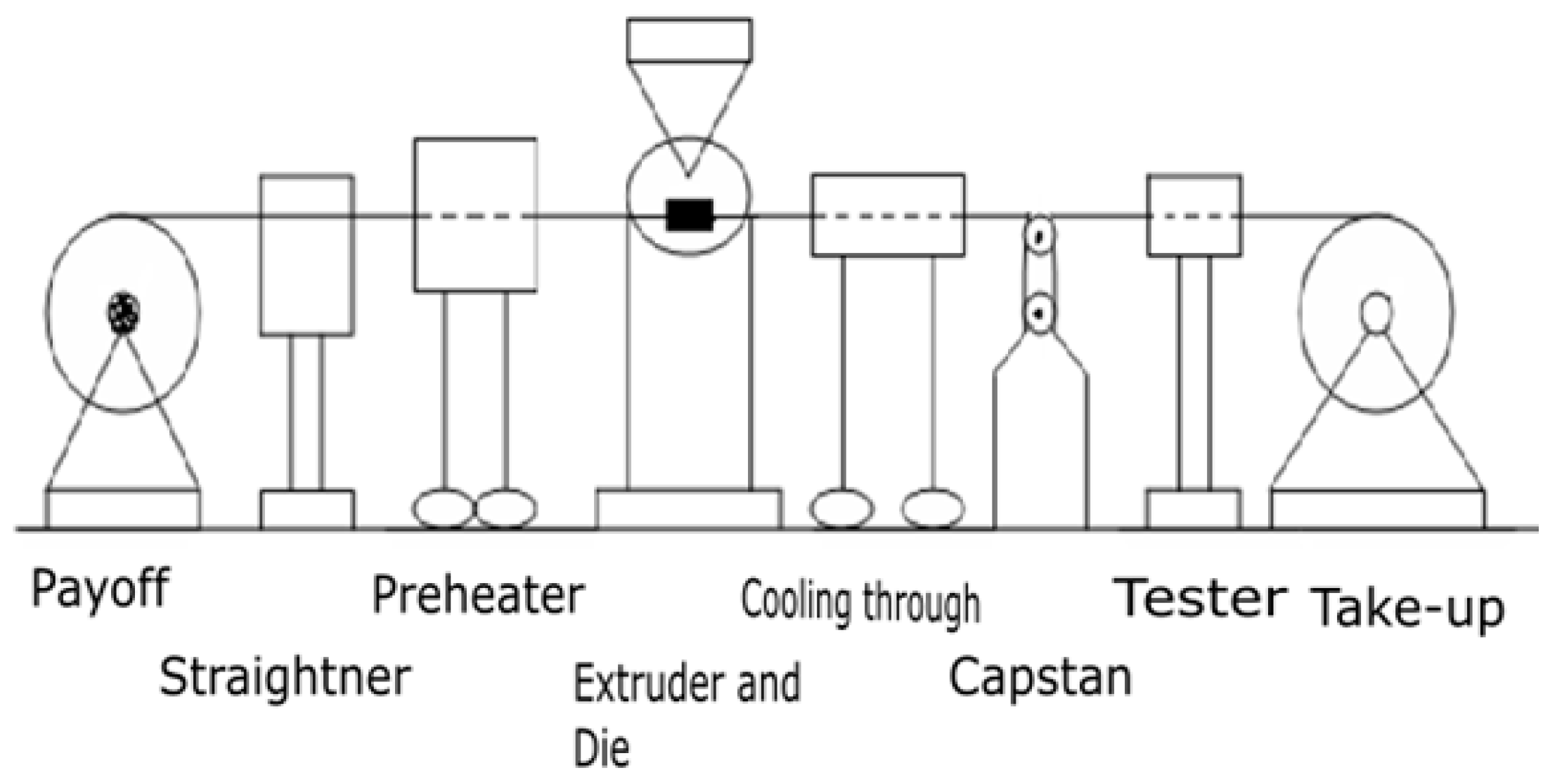
Wire-coating (an extrusion procedure) is generally utilized as part of the polymer industry for insulation and it protects the wire from mechanical damage. In this procedure, an exposed preheated fiber or wire is dipped and dragged through the melted polymer. This procedure can also be accomplished by extruding the melted polymer over a moving wire. Typical wire coating equipment is composed of five distinct units: Pay-off tool, wire pre-heating tool, an extruder, and a cooling and takeoff tool, as shown in Figure 1. The most common dies used for coatings are: Tubing-type dies and pressure type dies. The later one is normally used for wire-coating and seems like annulus. That is why flows through such die are similar to the flows through the annular area formed by a couple of coaxial cylinders. One of the two cylinders (inner cylinder) moves in the direction of the axial, while the second (external cylinder) is fixed. Preliminary efforts done by several researchers [5,6,7,8,9,10] used power-law and Newtonian models to reveal the rheology of the polymer melt flow.

At present, the Phan-Thein-Tranner (PTT) model, a third-grade visco-elastic fluid model, is the most commonly used model for wire-coating. The high-speed wire-coating process for polymer melts in the elastic constitutive model was analyzed by Binding in Reference [11]. It also discussed the shortcomings of the realistic modeling approach. Mutlu et al., in Reference [12], provided the wire-coating analysis based on the tube-tooling die. Kasajima and Ito, in Reference [13], meanwhile analyzed the wire-coating process and examined the post-treatment of the polymer extruded. They also discussed the impacts of heat transfer on the cooling coating. Afterward, Winter, in References [14,15], investigated the thermal effect on die, both from inside and outside perspectives. Recently, wire-coating in view of linear variations of temperature in the post-treatment analysis was investigated by Baag and Mishra in Reference [16].

The two-layer coatings process was also studied by many researchers. Kim et al. [17] used the WOW process for optical fiber coating. Zeeshan et al. [18,19] used pressure coating die for the two-layer coating in optical fiber analysis using the PTT fluid model. The same author discussed viscoelastic fluid for the two-layer coating in the fiber coating [20]. The Sisko fluid model was used for fiber coating by adopting the WOW process [21] in the presence of pressure type coating die.

In the present study, two-layer analysis is performed using viscoelastic fluid for optical fiber coating phenomenon in the presence of pressure type coating die. Moreover, the computation of heat transfer in fiber coating has significant effects on the operating variables in coating analysis. 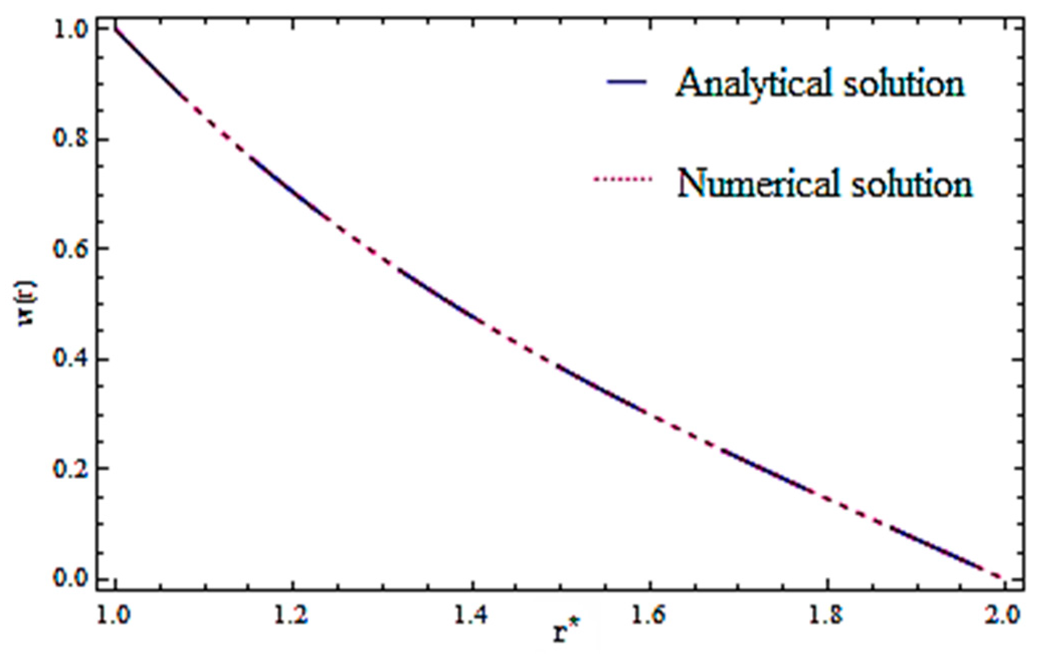The heat transfer also provides information to the die designers about the thermal variables that are important in obtaining better product quality and achieving optimum operating conditions [22,23,24,25]. The closed form solution for velocity field, thickness of the coated fiber optics, and temperature distribution has been obtained in the first case. In the second case, the numerical solution has been obtained. The results of both cases are compared and explained in detail. Finally, the recent result are also compared with the published work reported by Kim et al. [17], as a particular case and good agreement is found.

2. Analysis

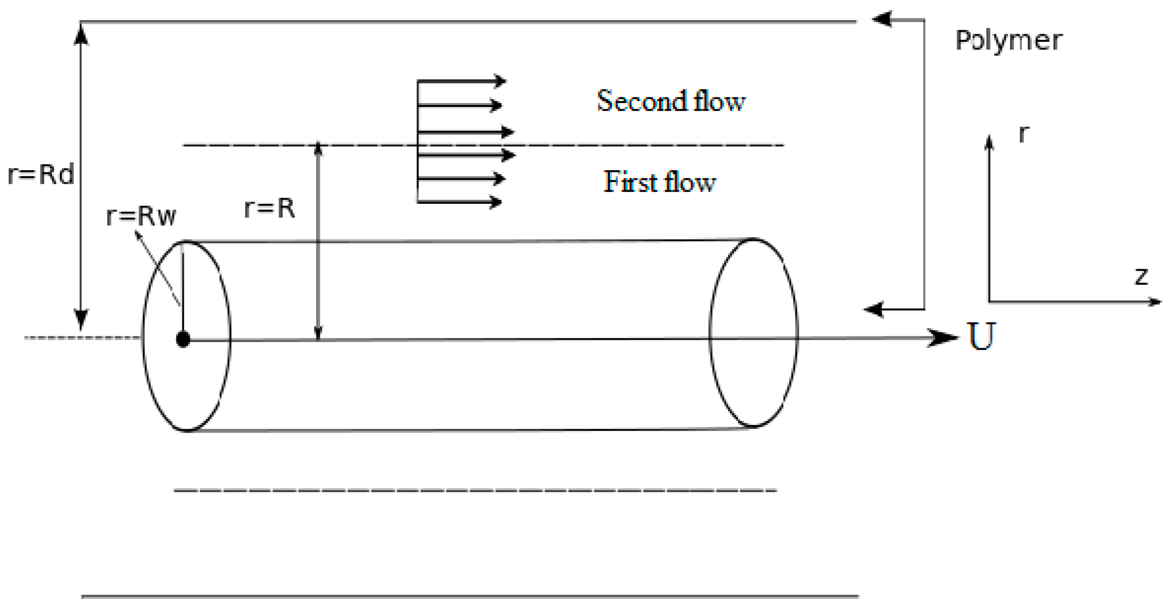
The WOW-type coating process is illustrated in Figure 2. The glass fiber is pulled with constant velocity $U$ through the primary coating die, which is filled with a primary coating resin. Afterwards, the uncured coated fiber optics enters the secondary coating die, which is filled with a secondary resin. After the secondary die the fiber leaves the system with two-coated layers, as displayed in Figure 2. At the end these coated-layers, they are cured by ultraviolet lamps. Where $R_w$, $R$, and $R_{\mathrm{d}}$ are the radius of the fiber optics, interface radius location, and radius of the die, $L$ is the length of the die. The present study is investigated under the assumption that the flow is incompressible, laminar, length of the die is sufficient large, the fiber optics moves along the centerline with constant speed, negligible small radial flow, as compared to the axial flow, because of high viscosity of the polymer-melt, the viscous impacts are dominant, as compared to the inertial effects, axial heat conduction is negligible, and the thermal conductivity, specific heat, melt density do not depend on the temperature and neglect the gravitational effect. To analyze the flow, the cylindrical coordinate system $\left(r,\mathsf{\theta },z\right)$ is used in which $r$ is the radial coordinate and $z$ is the axial coordinate of the wire means centerline of the die.

The basic equations governing the flow of incompressible fluids are:

$$\nabla .u=0$$

(1)

$$\mathsf{\rho }\frac{\mathrm{d}u}{\mathrm{d}t}=\nabla .\mathrm{T}$$

(2)

$$\rho c_p\frac{\mathrm{d}\Theta }{\mathrm{d}t}=k{\nabla }^2\Theta +\mathsf{\Phi }$$

(3)

$$f\left(trS\right)\mathrm{S}+\mathsf{\lambda }\dot{\mathrm{S}}=\mathsf{\eta }\mathrm{A}$$

(4)

where $\mathsf{\rho }$ is the density of the fluid, T is the shear stress tensor, c_p is the the specific heat, D/Dt denotes the material derivative, k is the thermal conductivity, Θ is the fluid temperature, Φ is the dissipation function, trS is the trace of extra stress tensor, $\dot{\mathrm{S}}$ is the upper contra-variant convicted tensor, μ is the viscosity of the fluid, and A is the deformation rate tensor.

The shear stress tensor is given in Equation (2) and the deformation rate tensor is given in Equation (4), defined as:

$$\mathrm{T}=-p\mathrm{I}+\mathrm{S}$$

(5)

$$\mathrm{A}=L^T+L$$

(6)

where I is the identity tensor and the superscript, T stands for the transpose of a matrix, and $L=\nabla u$.

The upper contra-variant convicted tensor $\dot{\mathrm{S}}$ in Equation (4) is given by

$$\dot{\mathrm{S}}=\frac{\mathrm{dS}}{\mathrm{d}t}-\left[{\left(\nabla u\right)}^T\mathrm{S}+\mathrm{S}\left(\nabla u\right)\right]$$

(7)

The function $f\left(tr\mathrm{S}\right)$ is given by Tanner [19,20,21],

$$f\left(trS\right)=1+\frac{\mathsf{\epsilon }\mathsf{\lambda }}{\mathsf{\eta }}\left(tr\mathrm{S}\right)$$

(8)

In Equation (8), $f\left(tr\mathrm{S}\right)$ is the stress function in which ε is related to the elongation behavior of the fluid. For ε = 0, the model reduces to the well-known Maxwell model and for λ = 0, the model reduces to a Newtonian one.

With the above frame of reference and assumptions the fluid velocity, extra stress tensor and temperature filed are considered as

$$u=\left(0,0,w\left(r\right)\right),\mathrm{S}=\mathrm{S}\left(r\right),\Theta =\Theta (r)$$

(9)

Using assumptions and Equation (9), the continuity Equation (1) satisfied identically and from Equations (2–8), we arrive at:

$$\frac{\partial p}{\partial r}=0$$

(10)

$$\frac{\partial p}{\partial \mathsf{\theta }}=0$$

(11)

$$\frac{\partial p}{\partial z}=\frac{1}{r}\frac{\mathrm{d}}{\mathrm{d}r}\left(r{S}_{\mathrm{rz}}\right)$$

(12)

$$k\left(\frac{{\mathrm{d}}^2}{\mathrm{d}{r}^2}+\frac{1}{r}\frac{\mathrm{d}}{\mathrm{d}r}\right)\Theta +S_{\mathrm{rz}}\frac{\mathrm{d}w}{\mathrm{d}r}=0$$

(13)

$$f\left(trS\right)S_{\mathrm{zz}}=2\mathsf{\lambda }{S}_{\mathrm{rz}}\frac{\mathrm{d}w}{\mathrm{d}r}$$

(14)

$$f\left(trS\right)S_{\mathrm{rz}}=\mathsf{\eta }\frac{\mathrm{d}w}{\mathrm{d}r}$$

(15)

$$\mathsf{\Phi }=S_{\mathrm{rz}}\frac{\mathrm{d}w}{\mathrm{d}r}$$

(16)

From Equations (10) and (11), it is concluded that $p$ is a function of $z$ only. Assuming that the pressure gradient along the axial direction is constant. Thus, we have $\raisebox{1ex}{$\mathrm{d}p$}\!\left/ \!\raisebox{-1ex}{$\mathrm{d}z$}\right.=\mathsf{\Omega }.$

Integrating Equation (12) with respect to $r$, we get

$$S_{\mathrm{rz}}=\frac{\Omega }{2}r+\frac{C}{r}$$

(17)

where C is an arbitrary constant of integration.

By substituting Equation (17) in Equation (15), we have

$$f\left(trS\right)=\frac{\mathsf{\eta }\frac{\mathrm{d}w}{\mathrm{d}r}}{\left(\frac{\Omega }{2}r+\frac{C}{r}\right)}$$

(18)

Combining Equations (14), (15) and (17), we obtain the explicit expression for a normal stress component $S_{\mathrm{zz}}$ as:

$$S_{\mathrm{zz}}=2\frac{\mathsf{\lambda }}{\mathsf{\eta }}{\left(\frac{\Omega }{2}r+\frac{C}{r}\right)}^2$$

(19)

From Equations (8) and (18), we have

$$\mathsf{\eta }\frac{\mathrm{d}w}{\mathrm{d}r}=\left(1+\mathsf{\epsilon }\frac{\mathsf{\lambda }}{\mathsf{\eta }}{S}_{zz}\right)\left(\frac{\Omega }{2}r+\frac{C}{r}\right)$$

(20)

Inserting Equation (19) in Equation (20), we obtain an analytical expression for axial velocity as:

$$\frac{\mathrm{d}{w}_{(j)}}{\mathrm{d}r}=\frac{1}{{\mathsf{\eta }}_{(j)}}\left(\frac{\Omega }{2}r+\frac{C_{(j)}}{r}\right)+2\mathsf{\epsilon }\frac{{\mathsf{\lambda }}^2}{{\mathsf{\eta }}^3{}_{(j)}}{\left(\frac{\Omega }{2}r+\frac{C_{(j)}}{r}\right)}^3$$

(21)

Additionally, the temperature distribution is

$$k_{(j)}\left(\frac{{\mathrm{d}}^2}{\mathrm{d}{r}^2}+\frac{1}{r}\frac{\mathrm{d}}{\mathrm{d}r}\right){\mathsf{\theta }}_{(j)}+S_{r{z}_{(j)}}\frac{\mathrm{d}{w}_{(j)}}{\mathrm{d}r}=0$$

(22)

Here, $j=1,2$ represents the primary layer and secondary layer flow, respectively.

The boundary condition on ${\mathsf{\theta }}_{(j)}$ is ${\mathsf{\theta }}_{\mathrm{w}}$ at the fiber optics and ${\mathsf{\theta }}_{\mathrm{d}}$ at the die wall. For the problem displayed in Figure 1, at the fluid interface, we utilize the assumptions that the velocity, the shear stress, and the pressure gradient along the flow direction and the temperature and the heat flux are continuous, which are given as follows.

The relevant boundary and interface conditions [17,18,19,20,21,22] on the velocity are

$$w_1=U\mathrm{at}r=R_{\mathrm{w}}\mathrm{and}{w}_2=0\mathrm{at}r=R_{\mathrm{d}}$$

(23)

$$w_1=w_2\mathrm{and}{S}_{\mathrm{rz}1}=S_{\mathrm{rz}2}\mathrm{at}r=R$$

(24)

The relevant boundary and interface conditions [17,18,19,20,21,22] on the temperature are

$${\mathsf{\theta }}_1={\mathsf{\theta }}_{\mathrm{w}}\mathrm{at}r=R_{\mathrm{w}}\mathrm{and}{\mathsf{\theta }}_2={\mathsf{\theta }}_{\mathrm{d}}\mathrm{at}r=R_{\mathrm{d}}$$

(25)

$${\mathsf{\theta }}_1={\mathsf{\theta }}_2\mathrm{and}{k}_1\frac{\mathrm{d}{\mathsf{\theta }}_1}{\mathrm{d}r}=k_2\frac{\mathrm{d}{\mathsf{\theta }}_2}{\mathrm{d}r}\mathrm{at}r=R$$

(26)

We introduce the non-dimensional flow variables as

$$\begin{gathered} r^{*}=\frac{r}{R_{\mathrm{w}}},w_{(j)}^{*}=\frac{w_{(j)}}{U},{\mathsf{\theta }}_{(j)}^{*}=\frac{{\mathsf{\theta }}_{(j)}-{\mathsf{\theta }}_{\mathrm{d}}}{{\mathsf{\theta }}_{\mathrm{d}}-{\mathsf{\theta }}_{\mathrm{w}}},C_{(j)}^{*}=\frac{2C_{(j)}}{R_{\mathrm{w}}^2\Omega },B{r}_{(j)}=\frac{{\mathsf{\eta }}_{(j)}{U}^2}{k_{(j)}\left({\mathsf{\theta }}_{\mathrm{d}}-{\mathsf{\theta }}_{\mathrm{w}}\right)},\mathsf{\epsilon }{D}_{(j)}^2=\frac{\mathsf{\lambda }{U}_{\mathrm{c}}}{R_{\mathrm{w}}},{\mathsf{{\rm X}}}_{(j)}=\frac{U_{\mathrm{c}}}{U}, \\ {\Gamma }^{*}=\frac{R}{R_{\mathrm{w}}},\frac{R_{\mathrm{d}}}{R_{\mathrm{w}}}=\mathsf{\delta }>1,K=\frac{k_2}{k_1},j=1,2. \end{gathered}$$

(27)

$$\frac{\mathrm{d}{w}_{(j)}}{\mathrm{d}r}=-4r{X}_{(j)}-4C_{(j)}{X}_{(j)}\frac{1}{r}-128X_{(j)}\mathsf{\epsilon }{D}_{(j)}^2{r}^3-384X_{(j)}\mathsf{\epsilon }{D}_{(j)}^2{C}_{(j)}r-384X_{(j)}{C}^2{}_{(j)}\mathsf{\epsilon }{D}_{(j)}^2\frac{1}{r}-128C^3{}_{(j)}{X}_{(j)}\mathsf{\epsilon }{D}_{(j)}^2\frac{1}{r^3}$$

(28)

$$\frac{\mathrm{d}}{\mathrm{d}r}\left(r\frac{\mathrm{d}{\mathsf{\theta }}_{(j)}}{\mathrm{d}r}\right)-4B{r}_{(j)}{X}_{(j)}\left(r^2+C_{(j)}\right)\frac{\mathrm{d}{w}_{(j)}}{\mathrm{d}r}=0$$

(29)

$$w_1\left(1\right)=1,w_2\left(\mathsf{\delta }\right)=0$$

(30)

$$w_1(\Gamma )=w_2(\Gamma ),S_{\mathrm{rz}1}(\Gamma )=S_{\mathrm{rz}2}(\Gamma )$$

(31)

$${\mathsf{\theta }}_1(1)=0,{\mathsf{\theta }}_2(\mathsf{\delta })=1,{\mathsf{\theta }}_1(\Gamma )={\mathsf{\theta }}_2(\Gamma ),\frac{{\mathrm{d}\mathsf{\theta }}_1(\Gamma )}{\mathrm{d}r}=K\frac{{\mathrm{d}\mathsf{\theta }}_2(\Gamma )}{\mathrm{d}r}.$$

(32)

where $U_{\mathrm{c}}=\raisebox{1ex}{$-R_{\mathrm{w}}^2\mathsf{\Gamma }$}\!\left/ \!\raisebox{-1ex}{$8{\mathsf{\eta }}_{(j)}$}\right.$ is the characteristic velocity scale, and $\mathsf{\epsilon }{D}_{(j)}^2$ is the characteristic Deborah number based on velocity scale $U_{\mathrm{c}}$, $X_{(j)}$ has physical meaning of a non-dimensional pressure gradient and $B{r}_{(j)}$ is the Brinkman number. Here, $\Gamma$ is the dimensionless parameter that is the ratio of the radius of the liquid-liquid interface to the radius of the optical fiber and j = 1, 2 stands for primary and secondary coating layer flows, respectively.

3. Analytical Solution (Exact Solution)

Analytical solution is given in the Appendix A.

4. Numerical Solution

We shall solve the above equations numerically. For this purpose, the Runge–Kutta–Fehlberg method is employed. The computations are carried out for δ = 2. Before proceeding to the results and their discussion, we first validate our results of numerical solution for comparing them with the corresponding results based on exact solution (given in Appendix A). To this end, Figure 3 is prepared, which shows the velocity curve obtained through both numerical and exact solutions. This figure clearly demonstrates an excellent correlation between both the solutions. This establishes the confidence on both exact and numerical solutions and also on the results predicted by these solutions.

5. Results of Analysis and Discussion

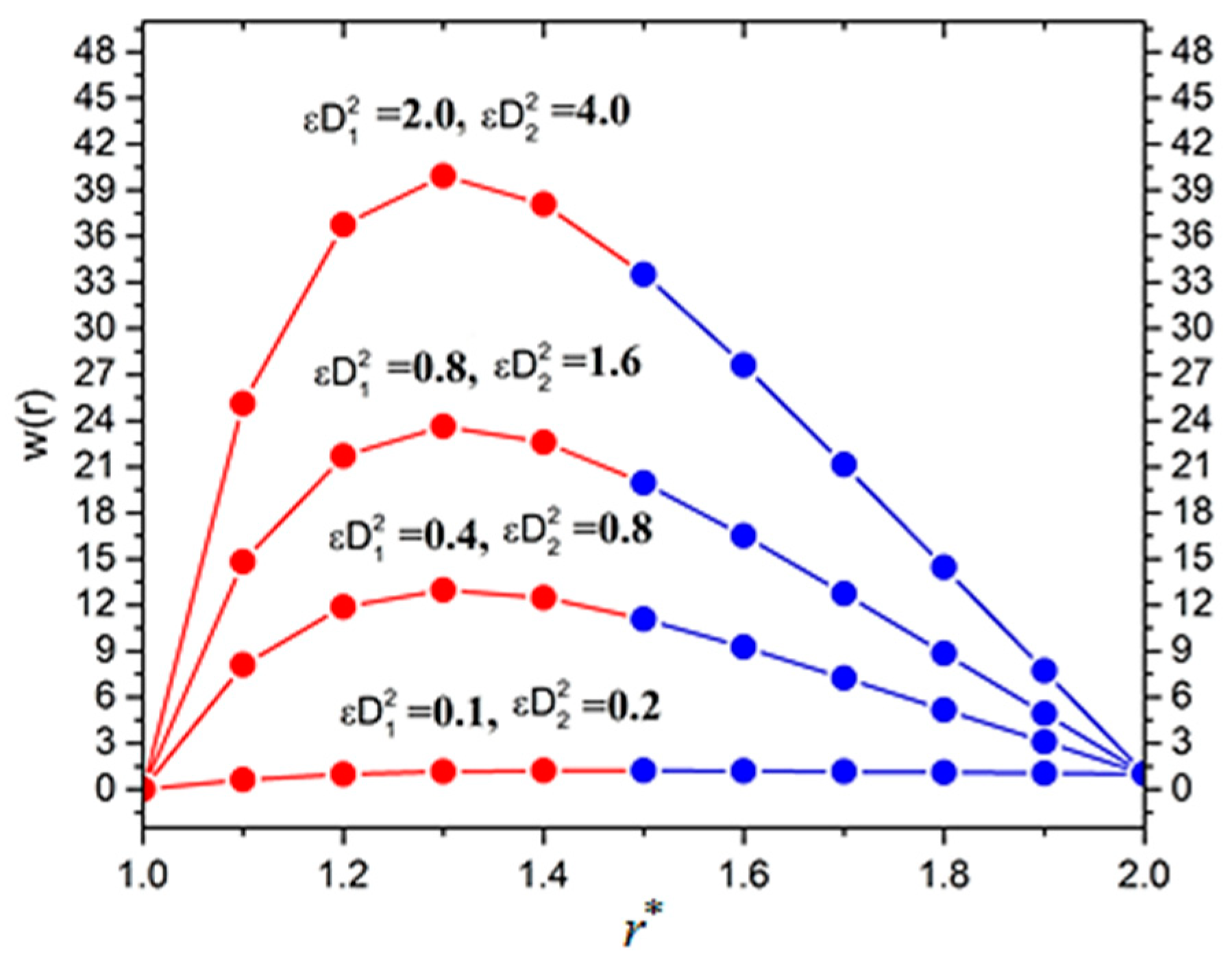
This section shows the impact of different emerging parameters of interest including the Deborah numbers (viscoelastic parameter) $\mathsf{\epsilon }{D}_1^2$ and $\mathsf{\epsilon }{D}_2^2$ ,pressure gradient parameters $X_1$ and $X_2$, Brinkman numbers $B{r}_1$ and$B{r}_2$ and the radii ration $\mathsf{\delta }$ on the velocity and temperature profiles, volume flow rate, thickness of the coated fiber optics, shear stress, and force required to pulling the fiber optics (later referred as force only). This purpose is achieved graphically in 4–11. 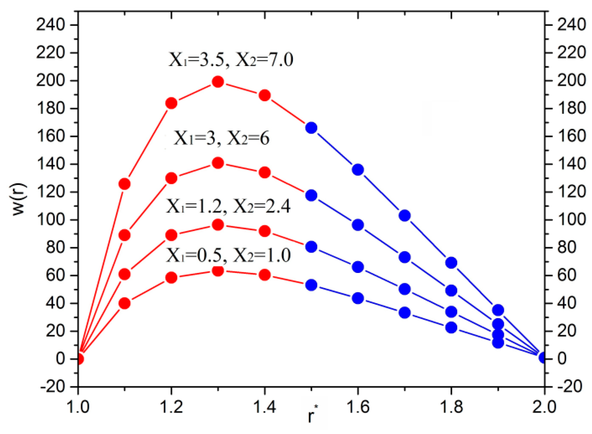Figure 4 shows the effect of dimensionless pressure gradient $X_1$ and $X_2$ on the velocity profile when $\mathsf{\epsilon }{D}_1^2$ = 0.5, $\mathsf{\epsilon }{D}_2^2$ = 1, $\mathsf{\delta }=2.$ This figure shows that, as the pressure gradient parameter increases, the velocity profile increases. The effect of Deborah number $\mathsf{\epsilon }{D}_1^2$ on velocity profile is shown in Figure 5. Since Deborah number is the measure of the ratio of the rate of the pressure drop in the flow to the viscosity, i.e., $\mathsf{\epsilon }{D}_{(j)}^2=\frac{\mathsf{\lambda }{U}_{\mathrm{c}}}{R_{\mathrm{w}}}$ where $U_{\mathrm{c}}=\raisebox{1ex}{$-R_{\mathrm{w}}^2\Omega $}\!\left/ \!\raisebox{-1ex}{$8{\mathsf{\eta }}_{(j)}$}\right.$ is the characteristic velocity and Ω is constant pressure gradient in the axial direction. That is why the velocity follows as an increasing trend with increasing Deborah number. From Figure 4 and Figure 5, it is clear that nonlinear behavior is occurred in the velocity profiles. Since the velocity of fluid first increase up to a certain value and then decreases, which shows the shear thickening effect. For low elasticity means for low Deborah number, the velocity disparity diverges a little from the Newtonian one, however, when the Deborah number is increased, these profiles turn into a more flattened one, showing the shear-thinning effect. It can be seen that, as $\mathsf{\epsilon }$ is reduced, the profiles turn to the Newtonian one and the result is therefore independent of$D_1^2\mathrm{and}{D}_2^2$. As $X_{(j)}=\frac{U_{\mathrm{c}}}{U}$ is the pressure gradient in which $U_{\mathrm{c}}=\raisebox{1ex}{$-R_{\mathrm{w}}^2\Omega $}\!\left/ \!\raisebox{-1ex}{$8{\mathsf{\eta }}_{(j)}$}\right.$ is the characteristic velocity where $U$ is the optical fiber velocity. That is why the velocity inside the die exceeds from the fiber optics velocity due to large values of the pressure gradient parameter.

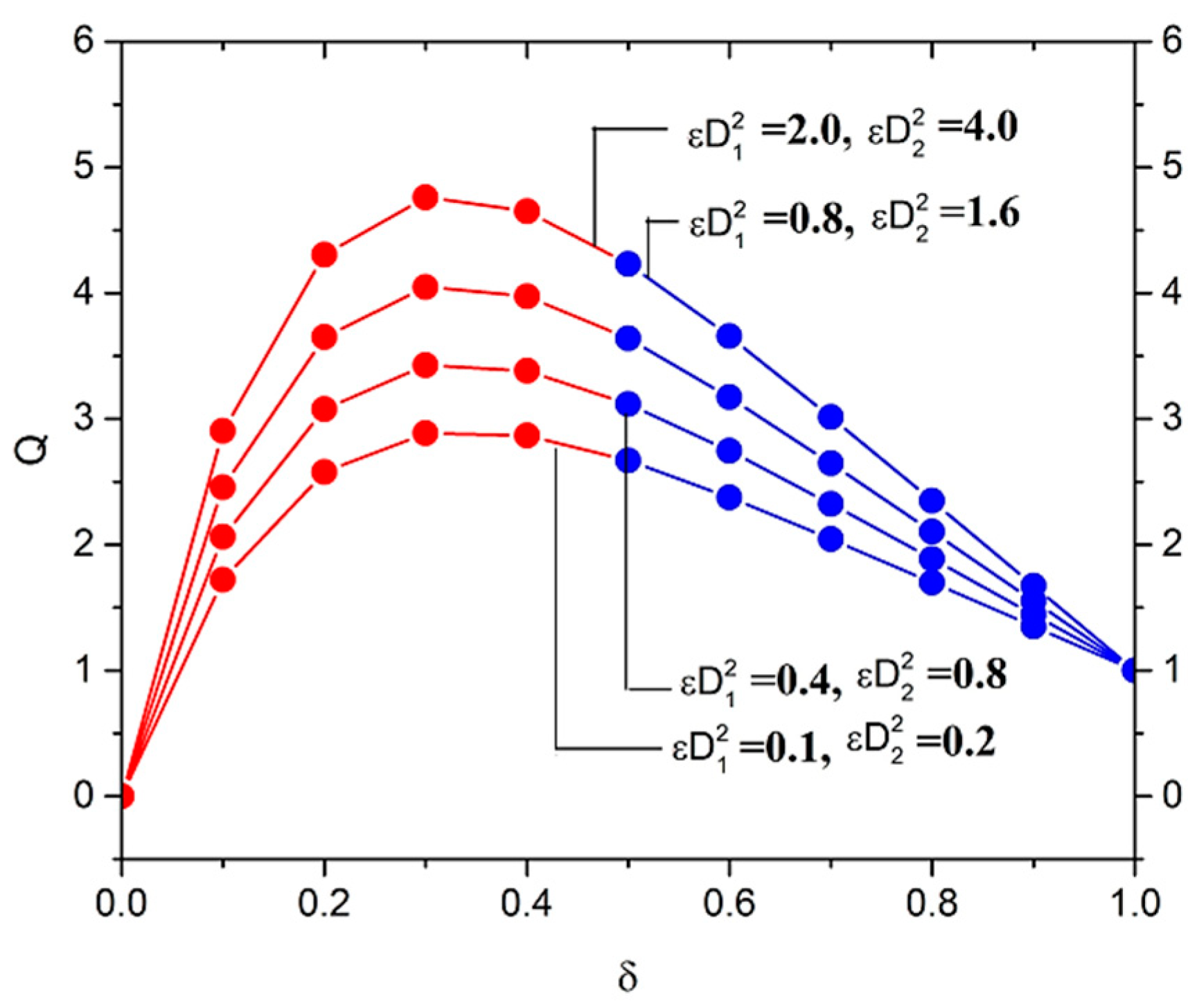
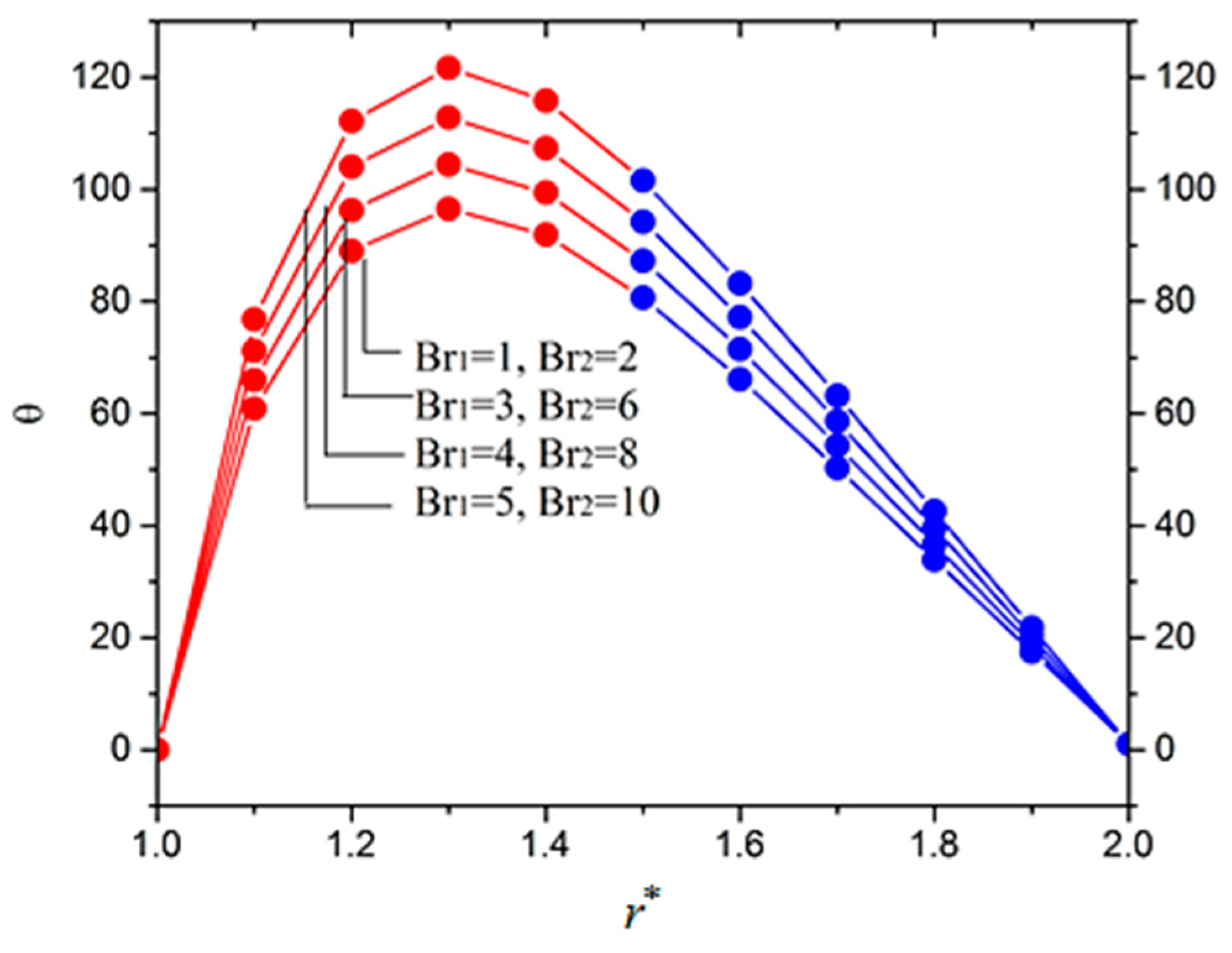
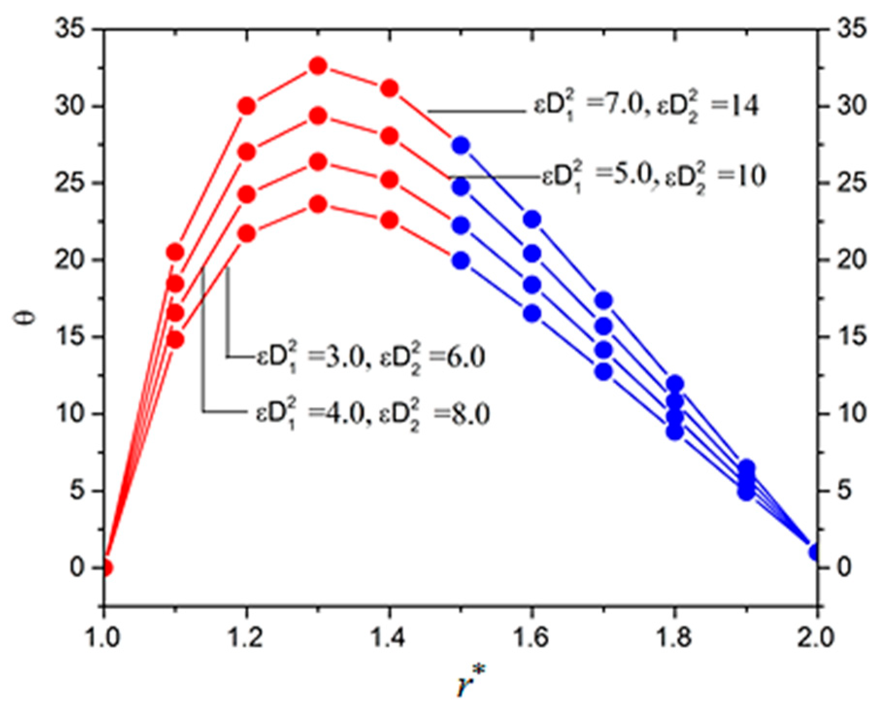
Figure 6 reveals that the volume flow rate increases with the increasing values of Deborah number along with increasing radii ratio $\mathsf{\delta }$. The dimensionless temperature profile inside the die for various values of emerging parameters is shown in Figure 7, Figure 8 and Figure 9. Figure 7 depicts the effect of Brinkman number on temperature profile. A rise in temperature is observed with increasing the Brinkman number. Additionally, the temperature increases with an increasing Deborah number and pressure gradient parameters, as shown in Figure 8 and Figure 9, respectively.

The thickness of the coated fiber optics or coating thickness (h_c) is shown in Figure 10 and Figure 11. It is observed that the thickness of the coated fiber optics increases with the increasing values of Deborah number and radii ratio $\mathsf{\delta }$, as shown in Figure 10 and Figure 11, respectively. For the sake of validity, the present work is also compared with the published work in Reference [17] and good agreement is found by taking the non-Newtonian parameter, which tends to zero, i.e., $\mathsf{\lambda }\to 0$.

6. Conclusions

To provide protection from signal attenuation and mechanical damage, optical fibers required a double-layer resin coating on the glass fiber. Wet-on-wet coating processes are considered for double-layer coating in optical fiber manufacturing. Expressions are presented for the radial variation of axial velocity and temperature distribution analytically and numerically. Analytical expressions of velocity, volume flow rate, final radius of the coated fiber optics and force required the full fiber optics, which are reported. The effect of physical parameters such as Deborah number, dimensionless parameter, radii ratio $\mathsf{\delta }$ and Brinkman number has been obtained numerically. It was found that velocity increases with increasing values of these parameters. The volume flow rate increases with increasing Deborah number. The thickness of coated fiber optic increase with an increase in $\mathsf{\epsilon }{D}_1^2$, $\mathsf{\epsilon }{D}_2^2$, and $\mathsf{\delta }$. The temperature depends upon $B{r}_1, B{r}_2,\mathsf{\epsilon }{D}_1^2,\mathsf{\epsilon }{D}_1^2$, $X_1$, and $X_2,$ and it increases with increasing these parameters. For $\mathsf{\epsilon }=0$ and $\mathsf{\lambda }=0,$our results respectively, reduce to Maxwell and linear viscous model. According to the best of our knowledge, there is no previous literature about the discussed problem, which is our first attempt to handle this problem with two-layer coating flows.

References

1. Rajagopal, K.R. On the boundary conditions for fluids of the differential type. In Navier-Stokes Equation and Related Non-Linear Problems; Sequira, A., Ed.; Plenum Press: New York, NY, USA, 1995; pp. 273–278. [Google Scholar]
2. Rajagopal, K.R.; Kaloni, P.N. Some remarks on the boundary conditions for fluids of the differential type. In Continuum Mechanics and its Applications; Gram, G.A., Malik, S.K., Eds.; Hemisphere: Washington, DC, USA, 1989; pp. 935–941. [Google Scholar]
3. Szeri, A.Z.; Rajagopal, K.R. Flow of a non-Newtonian fluid between heated parallel plates. Int. J. NonLinear Mech. 1985, 20, 91–101. [Google Scholar] [CrossRef]
4. Makinde, O.D. Irreversibility analysis for gravitry driven non-Newtonian liquid film along an inclined isothermal plate. Phys. Scr. 2006, 74, 642–645. [Google Scholar] [CrossRef]
5. Bernhardt, E.C. Processing of Thermoplastic Materials; Reinhold Publishing: New York, NY, USA, 1962; pp. 263–269. [Google Scholar]
6. McKelvey, J.M. Polymer Processing; John Wiley and Sons: New York, NY, USA, 1962. [Google Scholar]
7. Bagley, E.B.; Storey, S.H. Processing of thermoplastic materials. Wire Wire Prod. 1963, 38, 1104–1122. [Google Scholar]
8. Han, C.D.; Rao, D. The rheology of wire coating extrusion. Polym. Eng. Sci. 1978, 18, 1019–1029. [Google Scholar] [CrossRef]
9. Carley, J.F.; Endo, T.; Krantz, W. Realistic analysis of flow in wire coating dies. Polym. Eng. Sci. 1979, 19, 1178–1187. [Google Scholar] [CrossRef]
10. Han, C.D. Rheology and Processing of Polymeric Materials Volume 2 Polymer Processing; Oxford University Press: Oxford, UK, 2007; pp. 235–256. [Google Scholar]
11. Binding, D.M.; Blythe, A.R.; Guster, S.; Mosquera, A.A.; Townsend, P.; Wester, M.P. Modelling polymer melt flows in wire coating process. J. Nonnewton. Fluid Mech. 1996, 64, 191–206. [Google Scholar] [CrossRef]
12. Multu, I.; Twnsend, P.; Webster, M.F. Simulation of cable-coating viscoelastic flow with coupled and de-coupled schemes. J. Nonnewton. Fluid Mech. 1998, 74, 1–23. [Google Scholar] [CrossRef]
13. Kasajima, M.; Ito, K. Post-treatment of polymer extrudate in wire coating. Appl. Polym. Symp. 1973, 20, 221–235. [Google Scholar]
14. Winter, H.H. SPE 36th ANTEC. Tech. Pap. 1977, 23, 462. [Google Scholar]
15. Symmons, G.R.; Hasmi, M.S.J.; Pervinmehr, H. Plasto-hydrodynamics die lesswire drawing theoretical treatments and experimental result. In Progress Reports in Conference in Developments in Drawing of Metals; North Holland: New York, NY, USA, 1992; pp. 54–62. [Google Scholar]
16. Baag, S.; Mishra, S.R. Power law model in post treatment analysis of wirecoating with linearly variable temperature. Am. J. Heat Mass Transf. 2015, 2, 89–107. [Google Scholar]
17. Kim, K.; Kwak, H.S.; Park, S.H.; Lee, Y.S. Theoretical prediction on double-layer coating in wet-on-wet optical fiber coating process. J. Coat. Technol. Res. 2011, 8, 35–44. [Google Scholar] [CrossRef]
18. Kim, K.J.; Kwak, H.S. Analytic Study of Non-Newtonian Double Layer Coating Liquid Flows in Optical Fiber Manufacturing. Trans. Tech. Publ. 2012, 224, 260–263. [Google Scholar] [CrossRef]
19. Zeeshan, K.; Shah, S.I. Double-layer Optical Fiber Coating Using Viscoelastic Phan-Thien-Tanner Fluid. N. Y. Sci. J. 2013, 6, 66–73. [Google Scholar]
20. Khan, Z.; Islam, S.; Shah, R.A.; Khan, I.; Gu, T. Exact Solution of PTT Fluid in Optical Fiber Coating Analysis using Two-layer Coating Flow. J. Appl. Environ. Biol. Sci. 2015, 5, 596–605. [Google Scholar]
21. Khan, Z.; Islam, S.; Shah, R.A. Flow and heat transfer of two immiscible fluids in double-layer optical fiber coating. J. Coat. Technol. Res. 2016, 13, 1055–1063. [Google Scholar] [CrossRef]
22. Hayat, T.; Saif, R.S.; Ellahi, R.; Taseer, M.Y.R.; Ahmad, B. Numerical study for Darcy-Forchheimer flow due to a curved stretching surface with Cattaneo-Christov heat flux and homogeneous-heterogeneous reactions. Results Phys. 2017, 7, 2886–2892. [Google Scholar] [CrossRef]
23. Hayat, T.; Saif, R.S.; Ellahi, R.; Taseer, M.Y.R.; Alsaedi, A. Simultaneous effects of melting heat and internal heat generation in stagnation point flow of Jeffrey fluid towards a nonlinear stretching surface with variable thickness. Int. J. Therm. Sci. 2018, 132, 344–354. [Google Scholar] [CrossRef]
24. Shehzad, N.; Zeeshan, A.; Ellahi, R.; Vafai, K. Convective heat transfer of nanofluid in a wavy channel: Buongiorno’s mathematical model. J. Mol. Liquids 2016, 222, 446–455. [Google Scholar] [CrossRef]
25. Ellahi, R.; Riaz, A. Analytical solutions for MHD flow in a third-grade fluid with variable viscosity. Math. Comput. Modell. 2010, 52, 1783–1793. [Google Scholar] [CrossRef]
Figure 1. Optical fiber coating process.
Coatings 09 00147 g001
Figure 2. Geometry of double-layer optical fiber coating in wet-on-wet coating process [17].
Coatings 09 00147 g002
Figure 3. Comparison of analytical and numerical solutions when ε D 1 2 = 5 , ε D 2 2 = 10 , X 1 = 0.5,   X 1 = 1.0 ,   δ = 2 .
Coatings 09 00147 g003
Figure 4. Effect of X 1 and X 2 on velocity when ε D 1 2 = 5 , ε D 2 2 = 10 , δ = 2 .
Coatings 09 00147 g004
Figure 5. Effect of ε D 1 2 and ε D 2 2 on velocity profile when X 1 =   0.5,   X 1 = 1.0 , δ = 2 .
Coatings 09 00147 g005
Figure 6. Effect of ε D 1 2 and ε D 2 2 on volume flow rate when X 1 =   0.5,   X 1 = 1.0 .
Coatings 09 00147 g006
Figure 7. Effect of B r 1 and B r 2 on temperature X 1 = 0.5,   X 1 = 1.0 , ε D 2 2 = 10 , δ = 2 .
Coatings 09 00147 g007
Figure 8. Effect of ε D 1 2 and ε D 2 2 on temperature B r 2 = 0.5 X 1 = 0.5,   X 1 = 1.0 , δ = 2 .
Coatings 09 00147 g008
Figure 9. Effect of X 1 and X 2 on temperature B r 2 = 0.5 , ε D 2 2 = 10 , δ = 2 .
Coatings 09 00147 g009
Figure 10. Effect of ε D 1 2 on thickness of coated fiber optics when X 1 = 0.5,   X 1 = 1.0 , δ = 2 .
Coatings 09 00147 g010
Figure 11. Effect of δ on thickness of coated fiber optics when X 1 = 0.5,   X 1 = 1.0 , ε D 2 2 = 10 .
Coatings 09 00147 g011