
Impact of Seasonal Variation in Climate on Water Quality of Old Woman Creek Watershed Ohio Using SWAT


1
Texas Institute for Applied Environmental Research (TIAER), Tarleton State University, Member of the Texas A&M System, Stephenville, TX 76401, USA
2
Norwegian Institute of Bioeconomy Research, 1430 Ås, Norway
3
Department of Geology, Kent State University, Kent, OH 44240, USA
*
Author to whom correspondence should be addressed.
Climate 2021, 9(3), 50; https://doi.org/10.3390/cli9030050
Submission received: 31 December 2020
/
Revised: 15 March 2021
/
Accepted: 17 March 2021
/
Published: 19 March 2021
(This article belongs to the Special Issue The Water Security and Management under Climate Change)
Abstract
:The effect of the projected 21st century climate change on water quality in Old Woman Creek (OWC) watershed was evaluated using the Soil and Water Assessment Tool (SWAT) and the precipitation and temperature projections from three best Global Climate Circulation Model (GCM)l ensemble downloaded from the Coupled Model Intercomparison Project Phase 5 (CMIP5). These three best GCMs (GFDL-ESM2M, MPI-ESM-MR, EC-EARTH) were identified as those closest to the multivariate ensemble average of twenty different GCM-driven SWAT simulations. Seasonal analysis was undertaken in historical (1985–2014), current to near future (2018–2045), mid-century (2046–2075), and late-century (2076–2100) climate windows. The hydrological model calibration was carried out using a multi-objective evolutionary algorithm and pareto optimization. Simulations were made for stream flow and nine water quality variables (sediment, organic nitrogen, organic phosphorus, mineral phosphorus, chlorophyll a, carbonaceous biochemical oxygen demand, dissolved oxygen, total nitrogen, and total phosphorus) of interest. The average of twenty different CMIP5-driven SWAT simulation results showed good correlation for all the 10 variables with the PRISM-driven SWAT simulation results in the historical climate window (1985–2014). For the historical period, the result shows an over-estimation of flow, sediment, and organic nitrogen from January to March in simulations with CMIP5 inputs, relative to simulations with PRISM input. For the other climate windows, the simulation results show a progressive increase in stream flow with peak flow month shifting from April to March. The expected seasonal changes in each water quality variable have implications for the OWC estuary and Lake Erie water quality.
1. Introduction
The rise in the earth’s surface temperature due to climate change observed in the last century has been projected into the 21st century. This temperature increase will further moisten the atmosphere and influence the water cycle [1]. Climate change is expected to have variable impact on water resources across the globe [2]. The effect of climate change on streamflow cannot be overemphasized because of its implications on agriculture, economy, flooding, and water quality. The projected effects of climate change and management practices on hydrological variables have been studied using several climate models and basin scale hydrological models [3,4]. Hydrological modeling based on general circulation models (GCMs) are used to simulate the future changes in streamflow under projected climate conditions [5,6]. GCMs are different in structure and composition and produce results with different levels of uncertainties. Some studies combine multiple GCM for simulations and some make simulations based on some selected GCM, but a good approach is to test the performance of different GCMs and select the best model that reduces the uncertainty. Githui et al. [7] used SWAT with Model for the Assessment of Greenhouse Gas-Induced Climate Change (MAGICC) and reported an increase in the streamflow with the projected climate change in western Kenya.
Stumpf et al. [8] extracted the cyanobacteria index from MERIS data to study the annual bloom of cyanobacteria in Lake Erie from 2002–2012. They found out that Maumee River supplies enough phosphorus concentration to Lake Erie for the cyanobacteria bloom and attributed the Spring discharge and phosphorus load to the bloom. They obtained results that agreed with other works on the modeling of the intensity of the cyanobacteria bloom using the nutrients and created models for bloom prediction.
In order to meet the national water quality goals, Martin et al. [9] developed five different models in SWAT to simulate the impacts of 18 different management practices on the nutrient transport from the Maumee river basin to Lake Erie over a time frame of 10 years. The five models agreed on practices that would reduce the quantity and concentration of phosphorus transport with some degree of uncertainty.
Kuwaja et al. [10] assessed the inherent uncertainty in the capability of climate models and hydrological models to forecast water discharge and nutrient transport in the Maumee River watershed for the period 2046–2065 by forcing five distinct SWAT models with six different climate models from the CMIP5 ensemble. They found out that the hydrologic models can create greater uncertainties than the climate models in water quality forecasts, because hydrologic models created greater uncertainty in total phosphorus and dissolved reactive phosphorus forecast, while the dominant source of uncertainty in total nitrogen forecast was attributed to the climate models. They discouraged the use of single hydrologic or climate models by decision makers.
This work attempts to build on the recommendation of previous studies within available resources by using multiple climate models, a single hydrologic model, and a multi-objective calibration approach. The goal was to determine the effect of the projected 21st century seasonal variation in climate on water quality in the Old Woman Creek (OWC) watershed. The hypothesis tested was that increased streamflow driven by seasonal and annual variation in precipitation and temperature will result in comparable linear decreases in water quality across the century. It involved testing the performance of each of the 20 GCMs from the Coupled Model Intercomparison Project Phase 5 (CMIP 5) and selecting the best three models for seasonal variation simulations. Analysis was done on 10 variables of interest for four climate windows, which include historical (1985–2014), current to near future (2018–2045), mid-century (2046–2075), and late century (2076–2100). The variables of interest are streamflow, sediment transport (TSS), organic nitrogen, organic phosphorus (particulate p), mineral phosphorus (soluble reactive p or SRP), chlorophyll a, carbonaceous biochemical oxygen demand (CBOD), dissolved oxygen, total nitrogen, and total phosphorus. The specific objectives are summarized below:
- To evaluate the performance of each of the twenty GCMs from CMIP5 ensemble using exploratory simulations, calculate Euclidean distance of each model result relative to the multivariate ensemble average, and select the best three GCM models defined as those closest to the multivariate ensemble average, because the multivariate ensemble average of the 20 CMIP5 results is consistent with the average of the PRISM results.
- To reproduce the Parameter-elevation Regressions on Independent Slopes Model (PRISM) data simulation results for the historical climate window using the average result of the simulation made with the best three CMIP5 models.
- To make simulations for the current to near, mid-century, and late-century climate windows using best three CMIP5 models.
2. Materials and Methods
2.1. Old Woman Creek (OWC) Watershed and Estuary
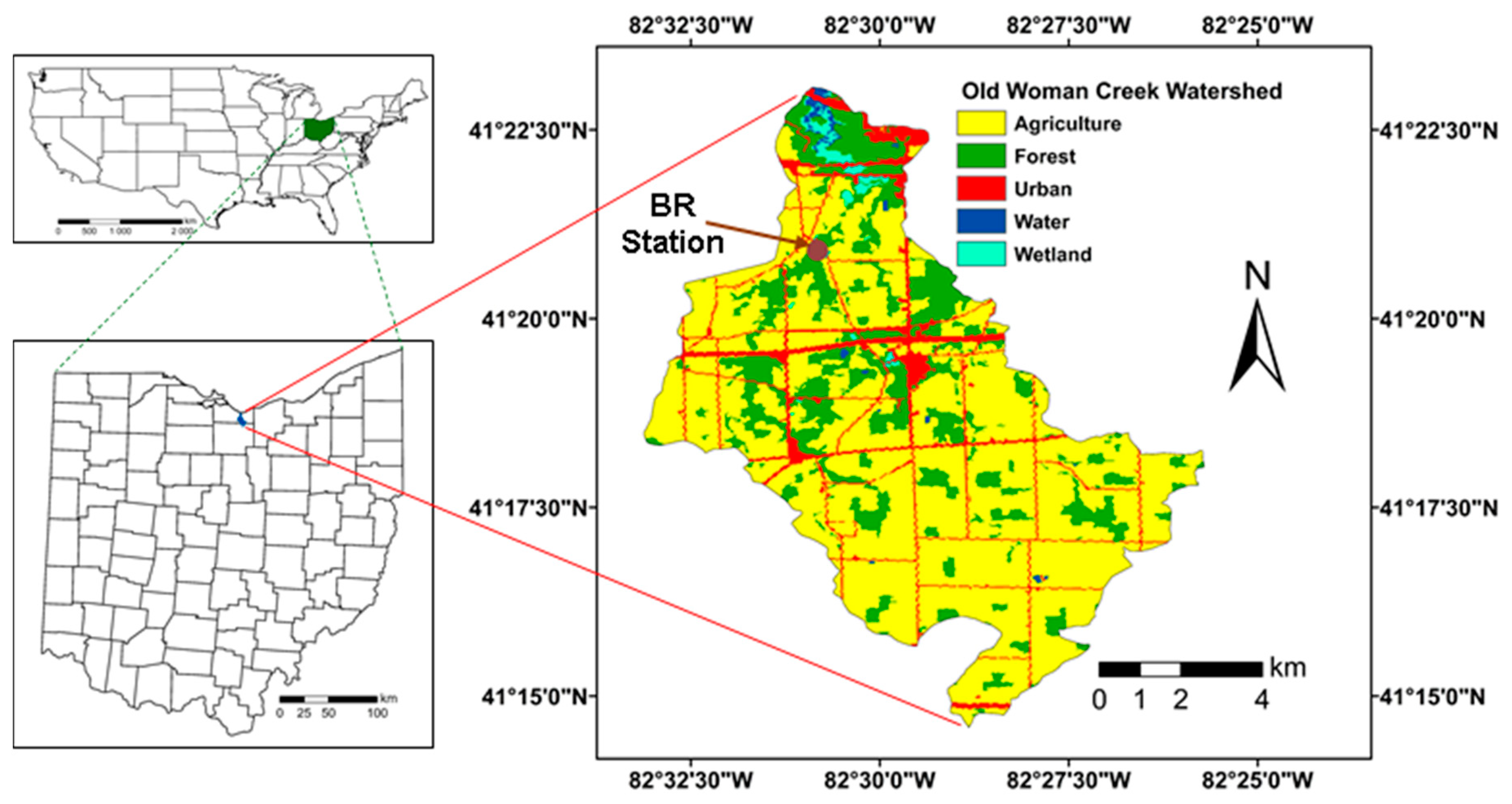
The OWC watershed drains a total land area of about 69 km2 with agriculture and forest as the dominant LULC. The Old Woman Creek (OWC) watershed has an estuary that was designated as the national estuarine research reserve (Latitude 41°23′ N, Longitude 82°33′ W). The OWC estuary is about 0.52 km2 in area; it consists of water, vegetation, swamps, marshes, and beach. It has a maximum width of 0.34 km, a mean depth of 0.4 km, and a depth of less than 1 m for the lower part, which can reach about 2 m around the mouth where the estuary empties into Lake Erie [11,12]. The OWC estuary is a freshwater estuary, within the OWC watershed, which maintains a natural habitat for aquatic life. It has extensive biological and physical diversity with various forms of terrestrial animals, aquatic animals, several species of birds, and habitat types [12]. There is diversity of phytoplankton notably the green algae, blue-green algae, and the diatoms [13]. The estuary helps in monitoring the water quality within the watershed and controls excessive flow of water during flooding (Figure 1). More than 60% of the watershed is used for agricultural purposes, which has implications on the water quality. Forest reserve occupies about 25%, while the remaining areas are wetlands and developed or built-up areas.
2.2. SWAT Data Acquisition and Preparation
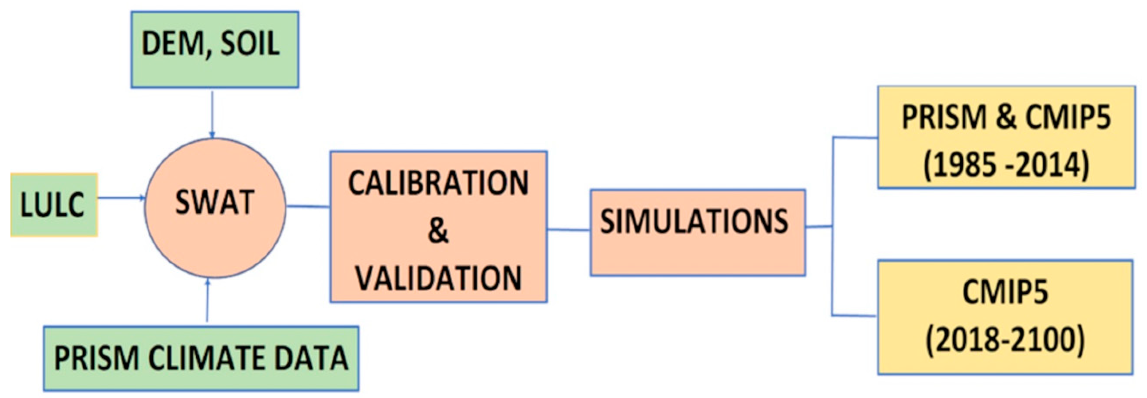
Data needed for hydrological modeling in SWAT include LULC data, digital elevation model (DEM), digital soil map, and climate and weather data. Ohio state 2001–2016 LULC data of 30 m resolution were downloaded from the National Land Cover Database website (https://www.mrlc.gov/data/type/land-cover, accessed on 15 March 2021) on 5 February 2019. Ohio area digital elevation model (DEM) of 10 m resolution was downloaded from the Geospatial Data Gateway (https://datagateway.nrcs.usda.gov, accessed on 15 March 2021). Digital soil map of Ohio, available at SSURGO (Soil Survey Geographic) database at https://www.nrcs.usda.gov, accessed on 15 March 2021, was downloaded for the analysis. The (PRISM) climate data of a spatial resolution of 4 × 4 km from 1981–2017 were downloaded from PRISM Climate Group at http://www.PRISM.oregonstate.edu/, accessed on 15 March 2021. The 20 different CMIP5 models of a spatial resolution ranging from latitude 1.25 to 2.7906 and longitude 1.125 to 3.75 from 1981–2100 were downloaded from the climate data store. The RCP 8.5 data for the 20 different Climate Model Intercomparison Project Phase 5 (CMIP5) ensemble were downloaded from the climate data store catalogue, downscaled, and biased-corrected for the hydrological model. Spatial interpolation method described by Flint and Flint [14] was used to extract the fine scale information from the coarse-scale information. The CMIP5 model was divided into historical (1981–2017) and future (2018–2100) data. The 4 km × 4 km grid resolution PRISM dataset for the historical period (1981–2017) was used for the spatial downscaling of the historical period data for the 20 CMIP5 models, and the climate parameters that were downscaled are the daily precipitation, minimum temperature, and maximum temperature. The historical (1981–2017) PRISM daily observed data were plotted against the simulated data to obtain the natural cubic regression splines used to generate the transfer functions, and this was applied to the CMIP5 future (2018–2100) data. The distribution-based scaling (DBS) method described by Yang et al. [15] was used to downscale the future (2018–2100) CMIP5 data to 4 km × 4 km grid resolution and bias-correct the data. All GIS layers were prepared with the OWC watershed shapefile. Stream discharge data were downloaded from the USGS national water information system (https://waterdata.usgs.gov/nwis/si, accessed on 15 March 2021) at station number 04199155. The water quality data for calibration and validation of the hydrological model were obtained from the water quality lab at Heidelberg University, Tiffin, Ohio. Hydrological modeling was carried out using the Soil and Water Assessment Tool (SWAT), which uses ArcMap as the graphical interface, available on Texas A&M University system website and installed as ArcSWAT. The method workflow is shown in Figure 2.
2.3. SWAT Model
The Soil and Water Assessment Tool (SWAT) is a basin scale hydrological modeling tool with the capability to model how land management will influence nutrient transport and, consequently, water quality in a large watershed with variable land management, soil types, and land use categories over a long period of time [16]. A detailed description of the different components of SWAT including pesticides application, management practices, crop growth, channel and reservoir routing, hydrology, sediment and nutrient transport, weather, and soil types and temperature can be found in Arnold et.al. [17]. SWAT is connected to the graphical platform (ArcGIS) using ArcSWAT for updating the spatial information such as stream network, management practices, weather data, soil data, and land use/cover maps into SWAT hydrological model [18,19]. The accuracy of the calibrated SWAT model was assessed using three statistical parameters, which compared the simulated to the observed values of the hydrological variables. They are percentage bias/percentage error [PBIAS (%)], Nash–Sutcliffe model efficiency (NSE) [20], and coefficient of determination (R2).
2.4. Calibration of SWAT Model
The setting up and parameterization of SWAT hydrological modeling for the OWC watershed was done in ArcSWAT 2012 interface. For the first stage, involving watershed delineation, drainage network establishment, and slope characterization, a 10 m digital elevation model (DEM) was prepared with the watershed shapefile and loaded. The digital stream network was displayed on the watershed DEM, the sub basin outlets were automatically generated using the minimum threshold approach, and an outlet was manually added at the location of the USGS gauge station at Berlin Road, where data were taken for SWAT calibration and validation. OWC watershed was delineated after the initial set up with an area of 66.9 km2 and 103 sub basins. To define the HRU and to hydrologically characterize the sub basins, DEM, land use, and soil data were used to create three slope classes: 0–3% for flat surfaces, 3–15% for moderate surfaces, and >15% for steep surfaces. Minor land use classes were eliminated by redistributing the smallest land use, slope, and soil classes occupying <10% of the sub basin over the larger ones, while keeping the entire modeling area of the sub basin at 100%. There is a total of 12 land use classes including open waters, developed open space, developed low intensity, developed medium intensity, developed high intensity, barren land, deciduous forest, evergreen forest, herbaceous, hay, cultivated crops, and woody wetlands. Complete HRU definition was done by reclassifying land use, soil, and slope to create 479 HRUs. Best management practices described by Confesor et al. and Scavia et al. [21,22] based on the three main crop types (soya, corn, and wheat) planted at OWC, tillage, planting and harvesting time, fertilizer application, etc., were encoded for each of the 479 HRUs in the SWAT model.
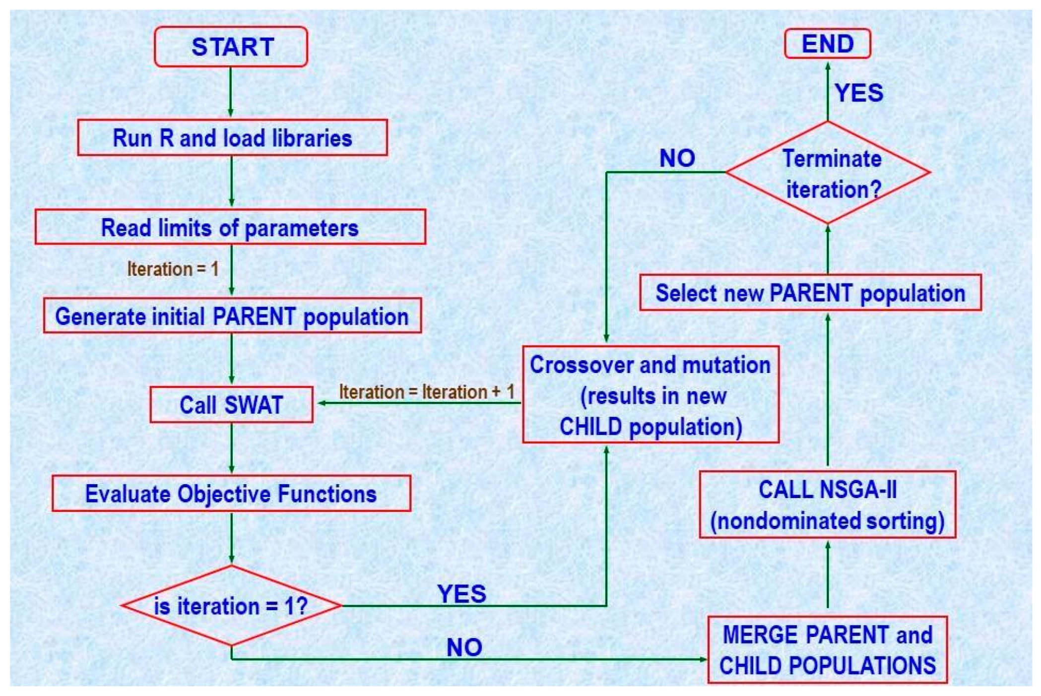
To prepare the model for calibration, PRISM climate data (1981–2017) were loaded, external climate data included precipitation and temperature (min, max, and daily average), while solar radiation, relative humidity, and wind speed were generated in SWAT for the hydrological model. Sensitivity analysis was done to determine the influence of the SWAT parameters on the water qualities variables and to select the most influential parameters for calibration [16], and a total of 56 SWAT parameters were selected to be optimized. The soil evaporation compensation factor was calibrated for each land use group, and each HRU was calibrated separately for the curve number to obtain 479 different curve numbers. The multi-objective calibration method developed by Confesor and Whittaker [23] (Figure 3) was modified and used for the optimization of the selected 56 SWAT parameters. The results of the sensitivity analysis and the hydrologic characteristics of the watershed assisted in fixing the limits of the optimized parameter for best model performance. The most complete record of daily streamflow found at USGS gaging station at Berlin Road in OWC ranged from 2015–2017, and this restricted the model calibration period to 5 May 2015–31 December 2016 (607 observations) and the validation period to 1 January 2017–31 December 2017 (365 observations).
In the calibration, the first 1000 solutions of the parent population were generated using the generic algorithm package (genalg) in R statistical language [24], and the five objective functions were applied to produce the child population. SWAT code was modified to run 200 iterations as a subroutine on IBM server with two quad-core processors to make a total of 201,000 SWAT runs for the calibration process.
2.5. Seasonal Analysis Simulations for Streamflow and Water Quality Variables
First, exploratory simulations were conducted with the PRISM data and the 20 different CMIP5 models across all the climate windows; the average of the 20 different CMIP5 model results was found to be consistent with the PRISM results across all the climate windows. The performance of each of the 20 CMIP5 models was evaluated by computing the Euclidean distance of each of the models relative to the overall model ensemble average, and the best three models were defined as those closest to the multivariate ensemble average, namely, GFDL-ESM2M, MPI-ESM-MR, and EC-EARTH were selected for the seasonal variation analysis.
In short, apart from the exploratory simulations, a total of 13 simulations was made, and the following tasks were performed to achieve the objectives:
- Evaluating the performance of each of the 20 CMIP5 climate models with respect to the overall average and selecting the best three CMIP5 models.
- Running one monthly simulation using PRISM climate data for the historical climate window.
- Running three monthly simulations using the best three CMIP5 climate models for the historical climate window.
- Comparing the average of the best three CMIP5 models’ simulation results to PRISM results for the historical climate window.
- Running nine monthly simulations consisting of three each for the current to near future, mid-century, and late-century climate windows using the best three CMIP5 climate models.
3. Results
3.1. Historical Climate Window (1985–2014) Results
3.1.1. Actual (PRISM) and Projected (CMIP5) Climate Forcing
The CMIP5 precipitation shows good agreement with the PRISM precipitation for most times of the year with slight under-estimation in the Fall and Summer and over-estimation between Winter and Spring with a phase lag. In PRISM data, the lowest (54.8 mm) and the highest (100.2 mm) precipitation were recorded in January and May, respectively, while in the CMIP5 model, the lowest (62.9 mm) and highest (97.8 mm) simulated precipitation occurred in February and June, respectively. The PRISM and CMIP5 temperature show almost perfect agreement across all seasons. The lowest and highest temperature in both PRISM (−3.08, 22.73 °C) and CMIP5 (−3.33, 22.75 °C) were observed in January and July, respectively.
3.1.2. PRISM and CMIP5 Streamflow and Water Quality Simulation Results (1985–2014)
The results of the monthly simulation for both PRISM data and CMIP5 models for streamflow and water quality variables are shown in Table 1. CMIP5 flow shows a similar trend to the PRISM flow and under-estimates flow for most part with slight over-estimation in February and March. In PRISM flow simulation, the lowest (0.24 m3/s) and highest (0.68 m3/s) flow were recorded in October and April, respectively, while in the CMIP5 flow result, the lowest (0.17 m3/s) and the highest (0.81 m3/s) simulated values occurred in September and February, respectively. The PRISM flow simulation appears to have dual peak flows (December and April), CMIP5 flow simulation has a peak flow in February. Analysis of the seasonal average for the flow of PRISM result shows that Spring has highest average of 0.61 m3/s, followed by Winter (0.58 m3/s), Summer (0.39 m3/s), and Fall (0.27 m3/s), and the same trend was recorded in CMIP5 results.
Sediment results for both PRISM and CMIP5 models bear good resemblance to the flow model, indicating that the flow controls the sediment transport. CMIP5 sediment curve shows slight under-estimation at the flanks and slight over-estimation from January to April. In PRISM sediment simulation, the lowest (198 tons) and highest (667 tons) sediment transport were observed in October and April, respectively, while in the CMIP5 sediment simulation, the lowest (109 tons) and the highest (797 tons) values were simulated in September and March, respectively. The PRISM sediment simulation curve has dual peak values (December and April), but the CMIP5 sediment simulation curve shows the peak transport in March. Seasonal average for sediment transport across the season in PRISM results shows that sediment transport was highest for Spring (1740 tons), followed by Winter (1601 tons), Summer (1041 tons), and Fall (640 tons) with the same pattern observed in CMIP5 results.
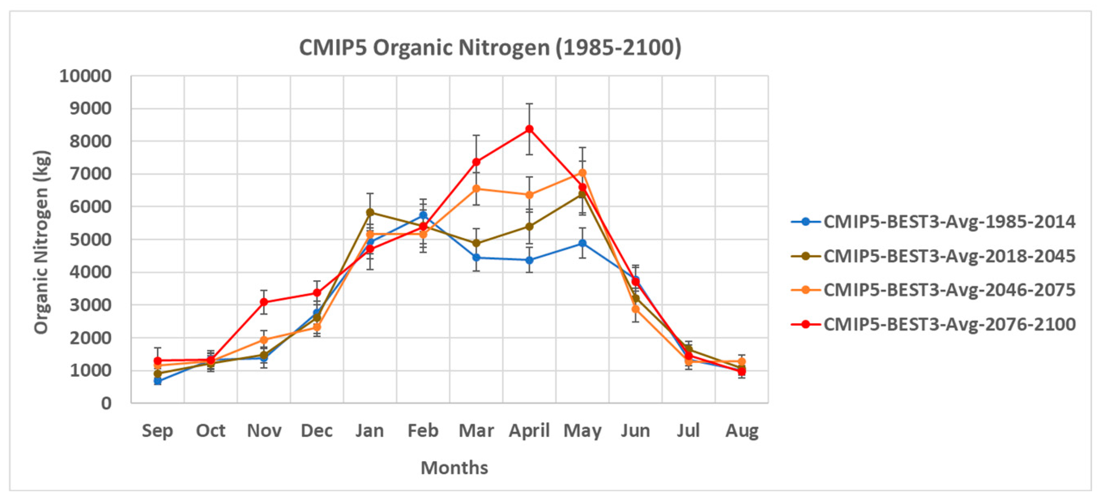
CMIP5 and PRISM organic nitrogen simulation shows the same trend with CMIP5 showing slight underestimation at the flanks of the curve and overestimation between December and April.
In PRISM organic nitrogen result, the lowest (1360 kg) and highest (4846 kg) organic nitrogen were recorded in October and May, respectively, while in the CMIP5 organic nitrogen result, the lowest (678 kg) and the highest (5736 kg) were simulated in September and February, respectively. Both PRISM and CMIP5 organic nitrogen simulations have dual peak organic nitrogen transport occurring in February and May. In both PRISM and CMIP5 results, the highest organic nitrogen transport was observed in Spring, followed by Winter, Summer, and Fall.
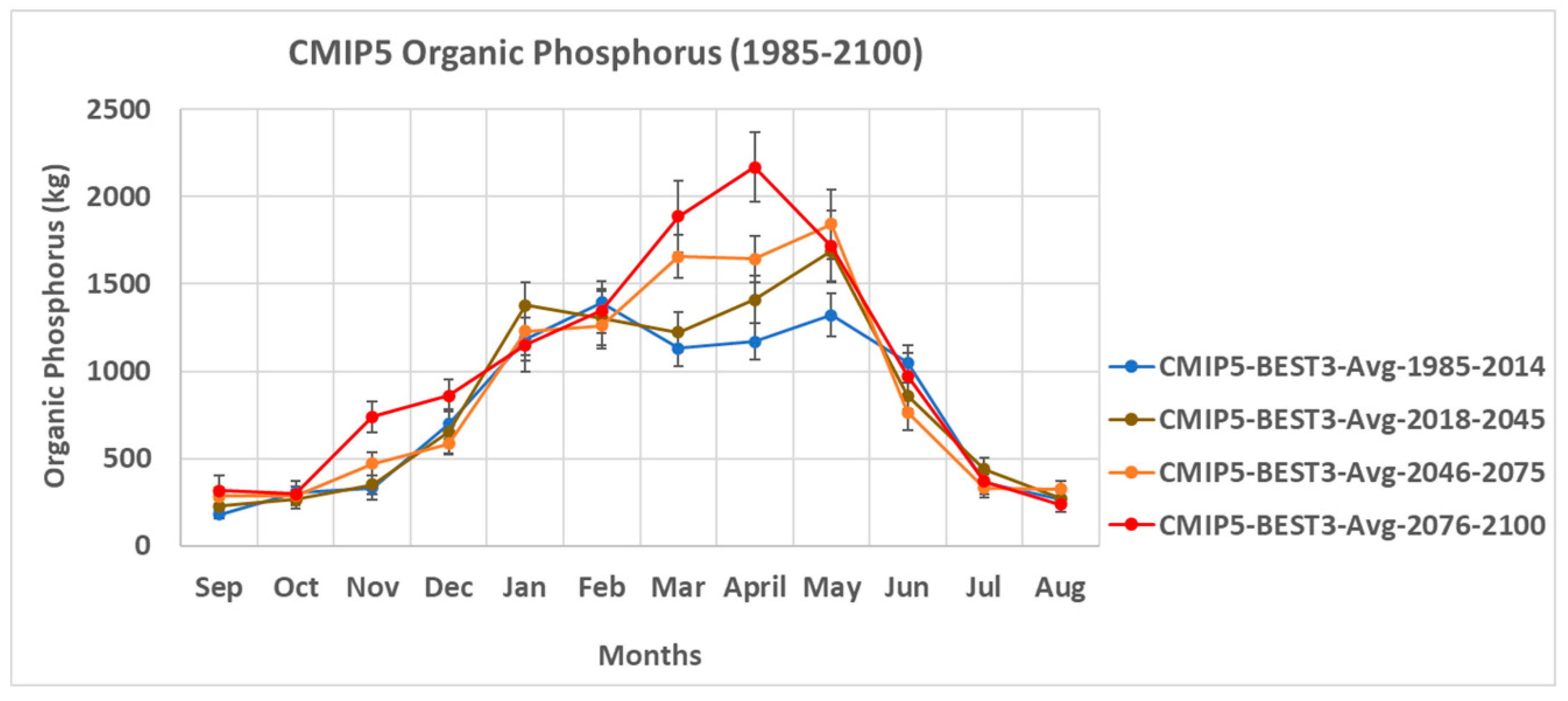
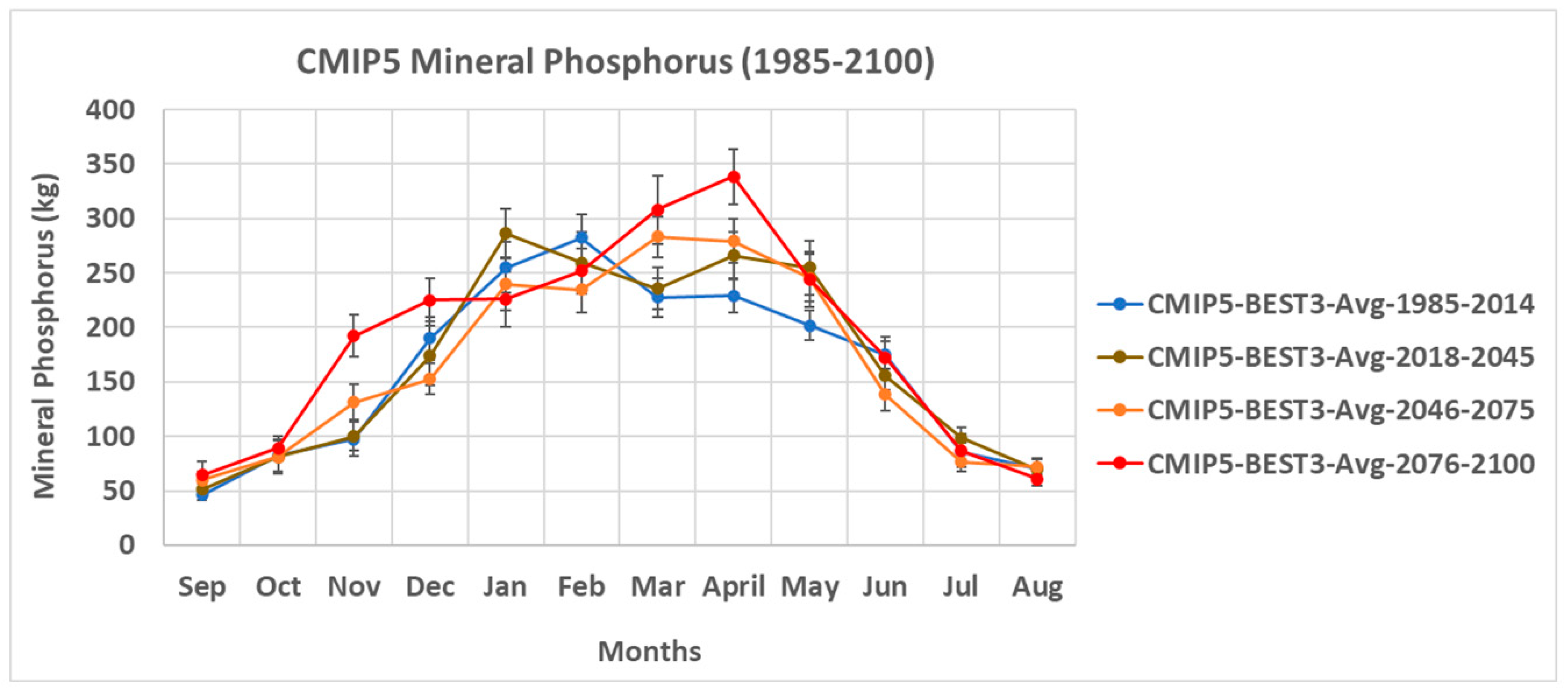
In organic phosphorus, mineral phosphorus, chlorophyll a, CBOD, and total nitrogen, CMIP5 results are similar to PRISM results with slight over-estimation from January to March. The results for the dissolved oxygen and organic nitrogen are very close across the year with CMIP5 over-estimating between February and March.
In all the variables including organic phosphorus, mineral phosphorus, chlorophyll a, CBOD, dissolved oxygen, total nitrogen, and total phosphorus, the statistics of the average of the best three CMIP5 results are similar to those of the PRISM results. This shows that the average of the best three CMIP5 models is able to reproduce the PRISM results within the error of SWAT simulation.
3.2. Future Climate Windows Results
3.2.1. Climate Forcing (CMIP5)
Because it has been established that the actual (PRISM) climate data are consistent with the projected (CMIP5) climate model for the OWC watershed, CMIP5 best three climate models were used for the simulations for the other three climate windows (2018–2045, 2046–2075, and 2076–2100).
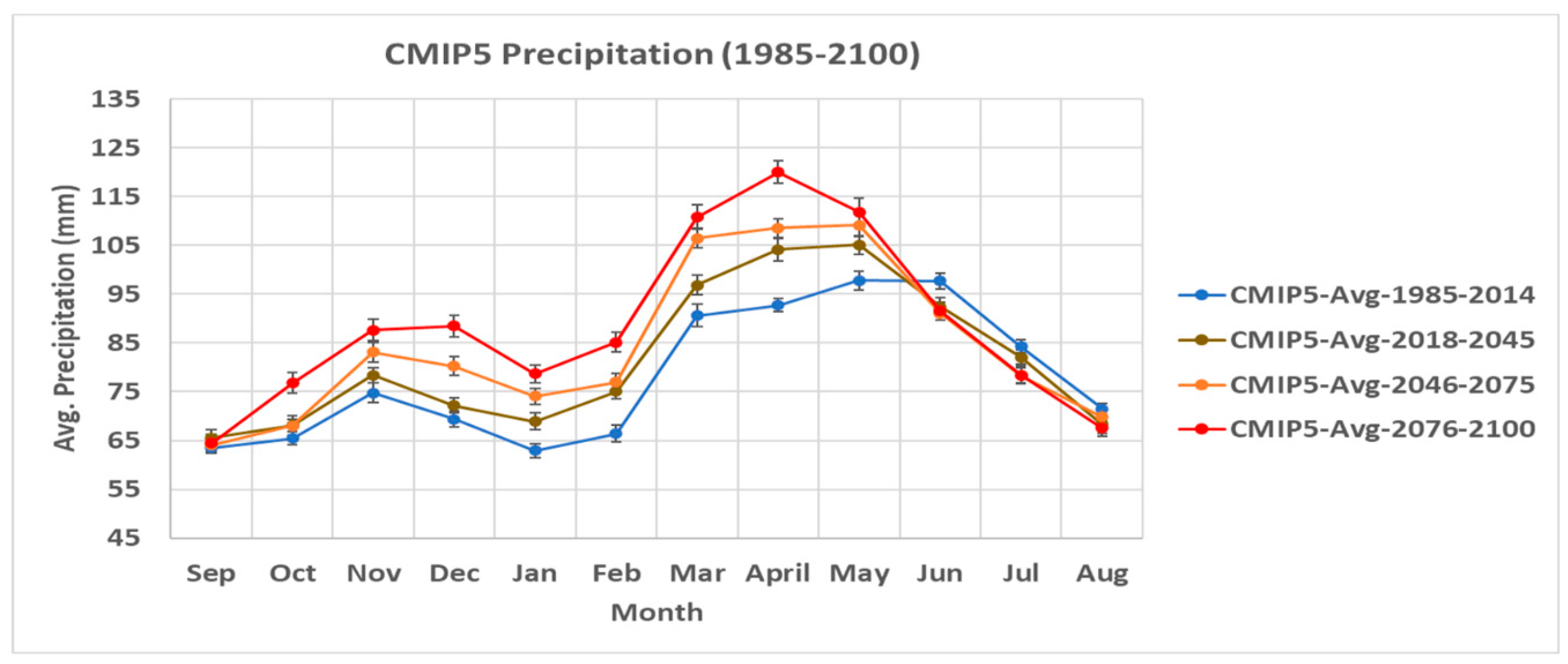
The CMIP5 projected precipitation for OWC watershed for the four climate windows from 1985–2100 is shown in Figure 4. In the current to future climate window and the mid-century climate window, the lowest and the highest precipitation were observed in September and May, respectively, but in the late-century climate window, the lowest and the highest precipitation were observed in September and April, respectively.
Analysis of seasonal average precipitation shows that in the current to future climate window, Spring has the highest precipitation (102 mm) followed by Summer (81 mm), Winter (72 mm), and Fall (71 mm). In the mid-century climate window, the highest precipitation (108 mm) was observed in Spring, followed by Summer (80 mm), Winter (77 mm), and Fall (72 mm). In the late-century climate window, Spring has the highest precipitation (114 mm) followed by Winter (84 mm), Summer (79 mm), and Fall (76 mm), indicating that the OWC watershed is expected to get wetter across the climate windows. Each of the climate windows shows one precipitation peak in Fall and another in Spring, with the Fall peak shifting from November in the historical climate window to December in the late-century climate window and the Spring peak shifting from June in the historical climate window to April in the late-century climate window. The lowest precipitation observed also shifts from January in the historical climate window to September in the late-century climate window.
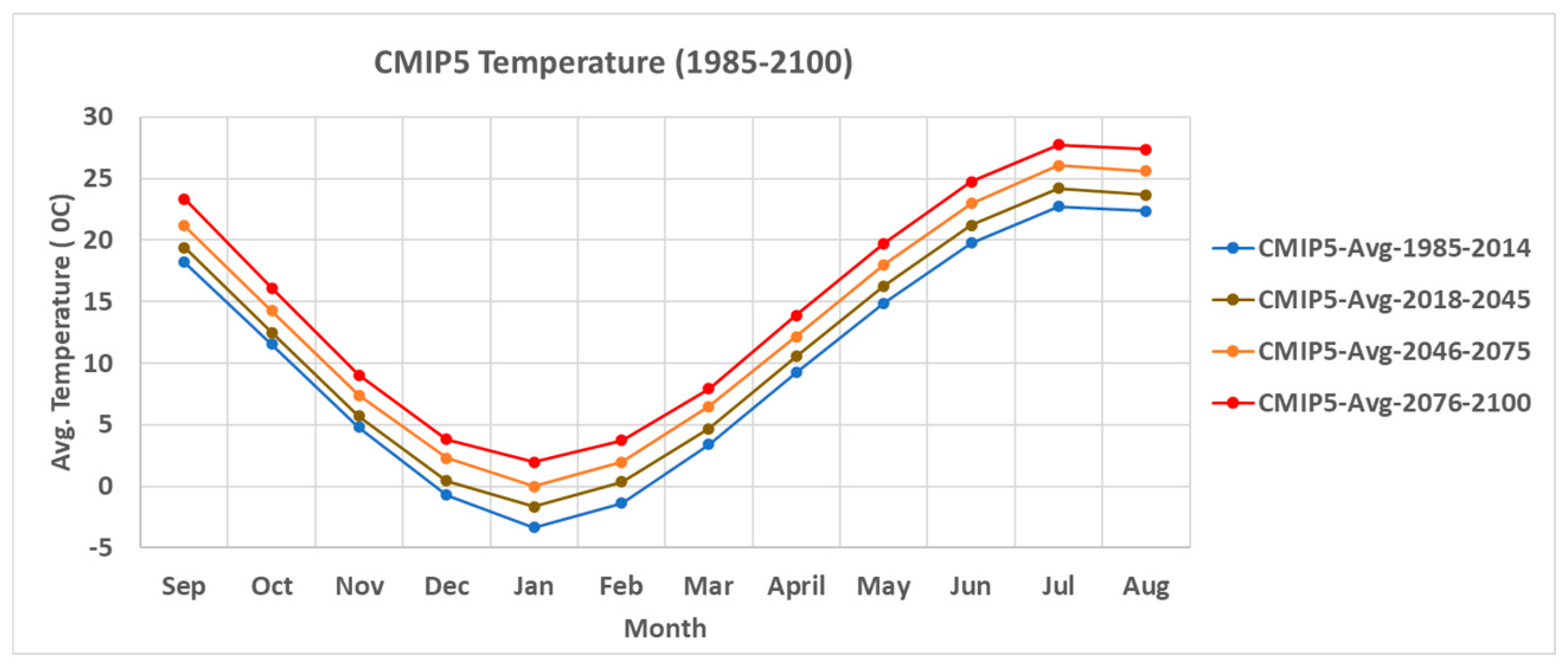
The CMIP5 projected temperature for the four climate windows from 1985–2100 is shown in Figure 5. The trend of the projected temperature is consistent across the seasons from the historical to the late-century climate window with the lowest temperature in January and the highest in July. The lowest and the highest temperatures observed across the climate windows are shown in Table 2. The seasonal warming pattern is consistent across the climate windows with Summer being the warmest, followed by Fall, Spring, and Winter. Both the coldest and the warmest season are projected to become warmer by the end of the century.
3.2.2. CMIP5 Streamflow and Water Quality Simulation Results (2018–2100)
The results of the simulation of streamflow and other water quality variables for the four climate windows are presented in Figure 6, Figure 7, Figure 8, Figure 9, Figure 10, Figure 11, Figure 12, Figure 13, Figure 14 and Figure 15. In streamflow results for the current to future climate window (Figure 6), the lowest and the highest streamflow were observed in October and April, respectively; in the mid-century and the late-century climate window, the lowest and the highest streamflow were observed in October and March, respectively, indicating an increase in projected streamflow across the climate windows and a shift in the peak flow from April to March.
The seasonal streamflow pattern is consistent across the climate windows. In the current to future climate window, Spring has the highest streamflow (0.84 m3/s) followed by Winter (0.69 m3/s), Summer (0.35 m3/s), and Fall (0.22 m3/s). In the mid-century climate window, the highest streamflow (0.96 m3/s) was observed in Spring, followed by Winter (0.68 m3/s), Summer (0.33 m3/s), and Fall (0.27 m3/s). In the late-century climate window, Spring has the highest streamflow (1.07 m3/s) followed by Winter (0.81 m3/s), Summer (0.37 m3/s), and Fall (0.33 m3/s). An increase in flow was also noticed between Fall and Winter across the climate windows.
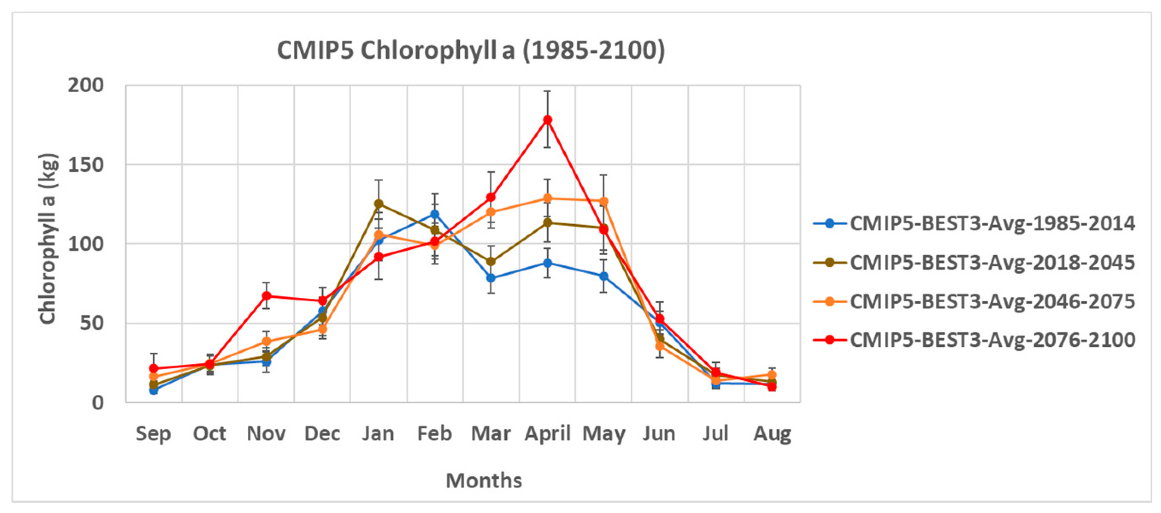
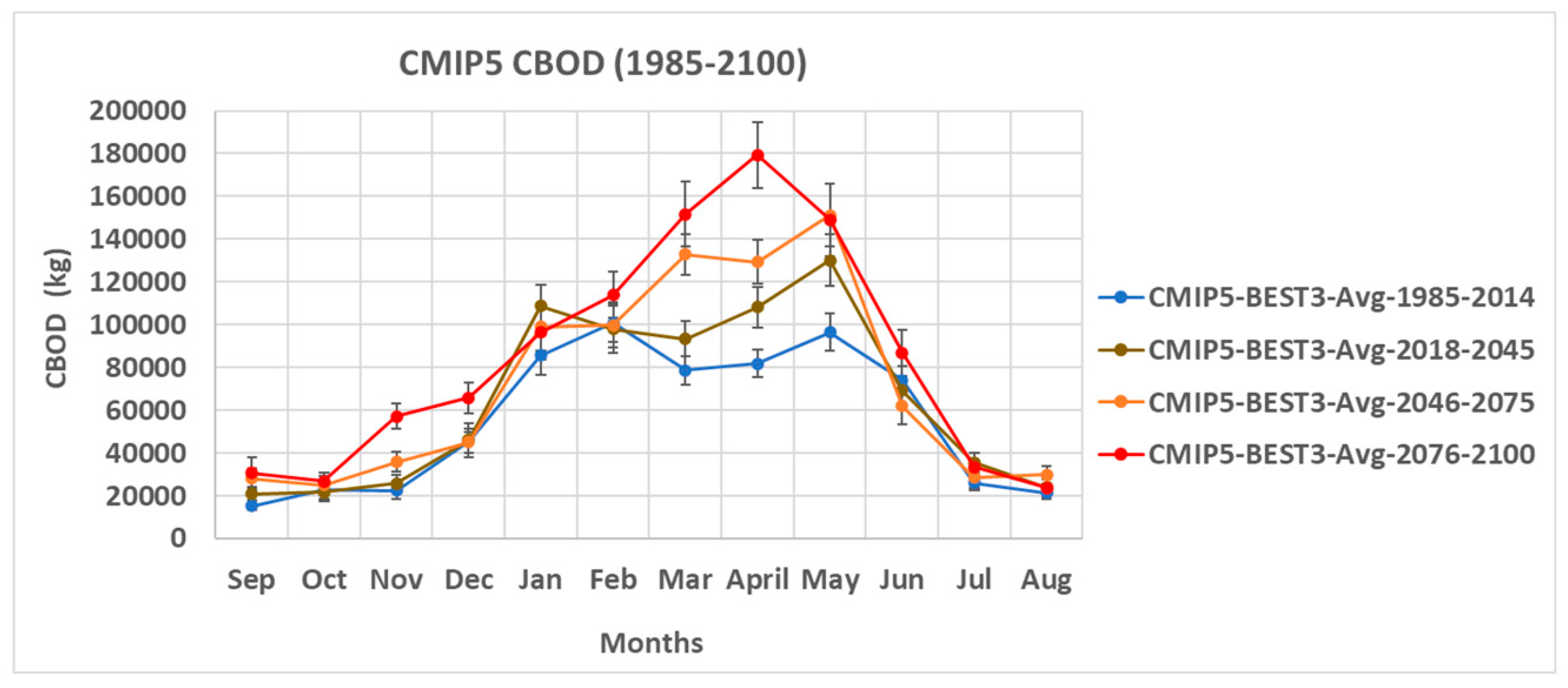
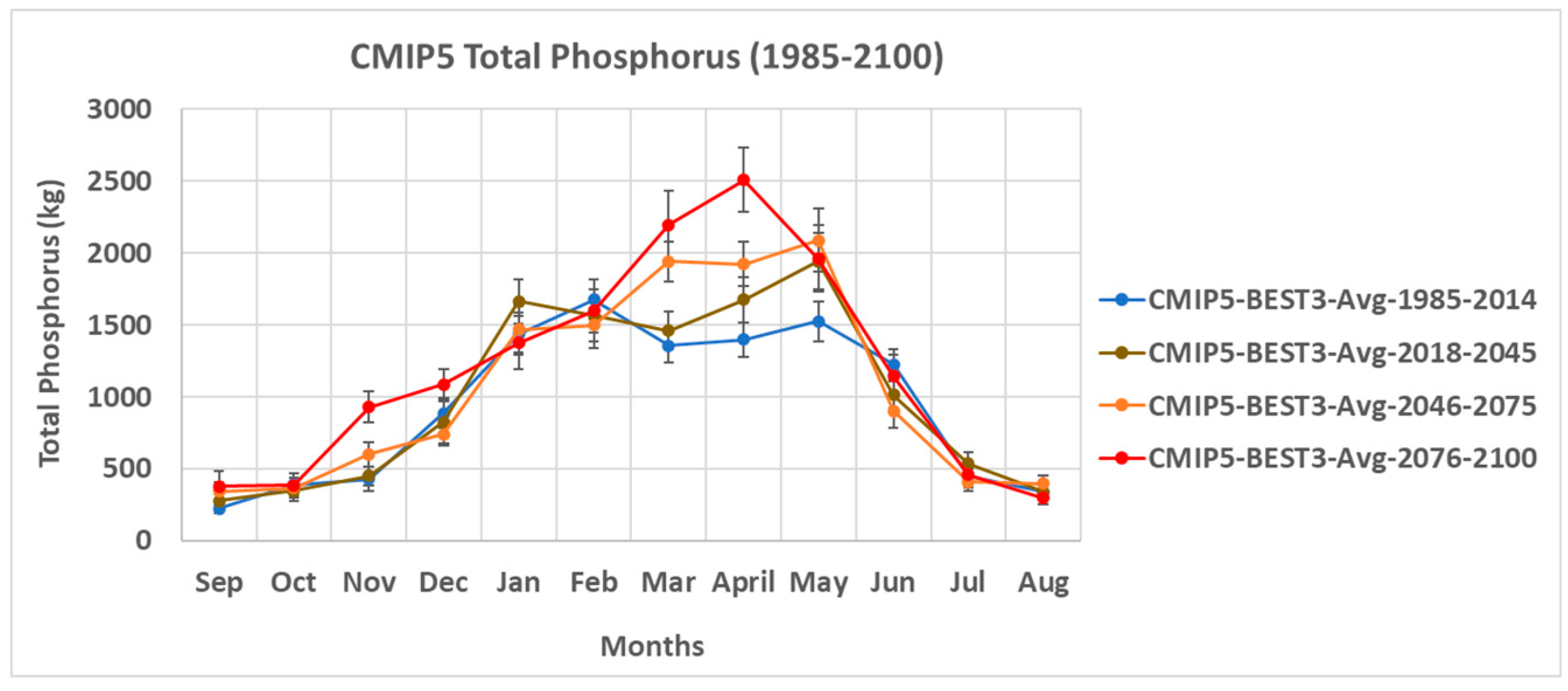
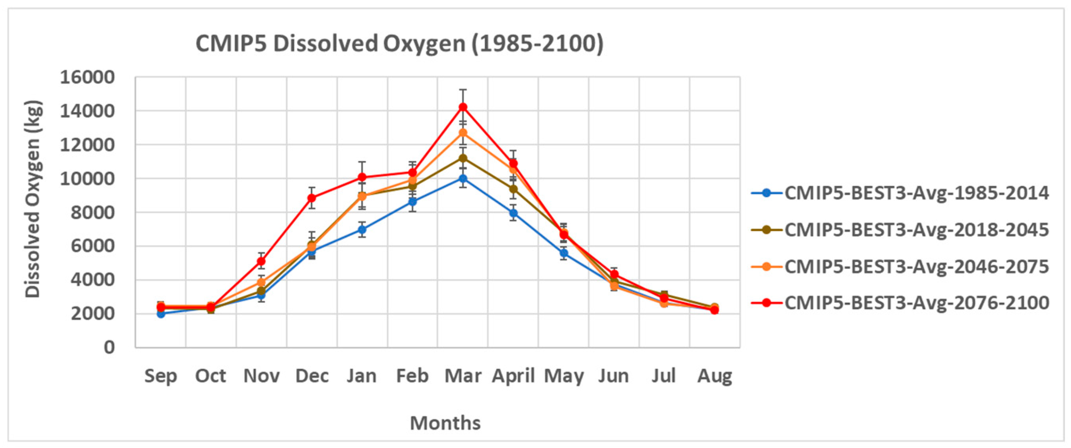
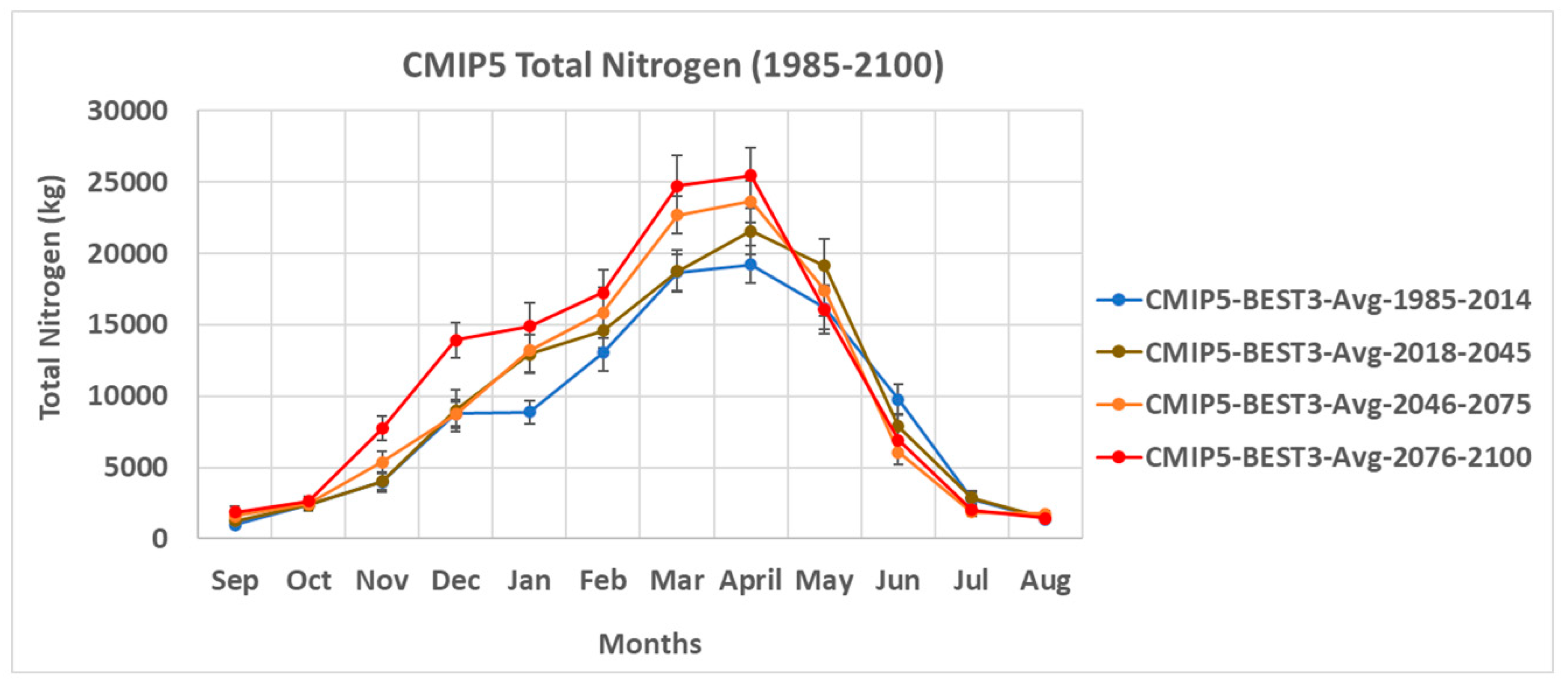
The sediment transport simulation results for the four climate windows bear almost perfect resemblance in trends to those of the streamflow (Figure 7). The peak and the lowest months are the same, and the seasonal pattern of sedimentation is the same as the seasonal pattern exhibited by streamflow. Organic nitrogen simulation results for the four climate windows are shown in Figure 8. The historical climate window has two peaks, in February and May; the current to future climate window has two peaks, in January and May; the mid-century climate window has two peaks, in March and May, while the late-century climate window has only one peak, in April. The lowest and the highest organic nitrogen transport values observed in the historical climate window were 678 and 5736 kg, respectively; in the current to future climate window these values were 909 and 6402 kg, respectively; in the mid-century climate window, the values were 1155 and 7043 kg, respectively, and in the late-century climate window, they were 957 and 8370 kg. A consistent seasonal transport pattern was observed across the four climate windows with Spring having the highest transport of organic nitrogen, followed by Winter, Summer, and Fall. Organic phosphorus, mineral phosphorus, chlorophyll a, CBOD, and total phosphorus have both Winter and Spring peaks in the first three climate windows with the Winter peak disappearing in the last climate window (Figure 9, Figure 10, Figure 11, Figure 12 and Figure 13). For dissolved oxygen and total nitrogen, the peak concentration month stays constant in March and April, respectively, with early Winter rise across the windows (Figure 14 and Figure 15).
3.2.3. Estimated Change in Simulated Variables across the Century (2018–2100)
The changes observed in flow and water quality variables across the century relative to the historical climate window are presented as percentages in Table 3, Table 4 and Table 5. In the current to future climate window (Table 3), seasonal average increased across all the simulated variables in the Fall and Spring with highest increase of 29.2% for CBOD and 26.0% for sediment in the Spring, and the lowest seasonal increase was observed in the Winter simulation for total phosphorus. Winter average also increased for all the simulated variables except for mineral phosphorus, while Summer average increased for flow, sediment, CBOD, and dissolved oxygen and decreased in other variables. The lowest seasonal decrease of −12.6% was observed in the Summer simulation for total nitrogen. There is an increase in the annual maximum and minimum for all the simulated variables relative to the historical climate window. The highest total annual increase of 19.4% was observed in sediment transport, followed by 16.4% in CBOD, and 15.3% in flow in the current to future climate window relative to the historical climate window
For the change observed in the mid-century climate window relative to the historical climate window (Table 4), the seasonal average further increased across all the simulated variables in the Fall and Spring with highest increase of 48.9% for sediment and 46.6% for CBOD in the Fall, and 61% for CBOD and 57.3% for sediment in the Spring, and the lowest seasonal increase was observed in the Summer simulation for flow. The Winter average increased in five variables and decreased in five variables, while the Summer average increased for flow and sediment but decreased in other variables. The lowest seasonal decrease of -15.3% was observed in the Summer simulation for organic phosphorus. The annual maximum and minimum values for all the simulated variables increased relative to the historical climate window. The highest total annual increase of 34.5% was observed in sediment transport, followed by 29.2% in CBOD relative to the historical climate window.
The late-century climate window has the largest change relative to the historical climate window. The seasonal average further increased across all the simulated variables in the Fall and Spring with the highest increase of 97.9% for sediment and 97.2% for CBOD in the Fall and 86.9% for CBOD and 81.2% for sediment in the Spring, and the lowest seasonal increase of 0.3% was observed in the Winter and Summer simulation for organic nitrogen. The Winter average increased in most variables except in mineral phosphorus and chlorophyll a, while the Summer average increased in most variables except in organic phosphorus, mineral phosphorus, total nitrogen, and total phosphorus. The lowest seasonal decrease of −25.6% was observed in the Summer simulation for total nitrogen. The annual maximum and minimum values for all the simulated variables increased relative to the historical climate window. The highest total annual increase of 62.0% was observed in sediment transport, followed by 51.3% in CBOD relative to the historical climate window. Though these increases are significant, a large portion of the increase would be transported into Lake Erie, while some will be retained in the OWC estuary to contribute to the water quality degradation.
In the current–future climate window, the projected change in precipitation of about +4.2% and temperature of about +12.9% relative to the historical climate window is expected to bring about an average annual increase of 15.3% in streamflow, 19.4% in sediment transport, 9.4% in organic nitrogen, 7.1% in organic phosphorus, 4.6% in mineral phosphorus, 11.7% in chlorophyll a, 16.4% in CBOD, 13.8% in dissolved oxygen, 9.2% in total nitrogen, and 6.7% in total phosphorus, relative to the level in the historical climate window. In the mid-century climate window, the projected change in precipitation of about +7.6% and temperature of about +30.1% relative to the historical climate window is expected to bring about an average annual increase of 23% in streamflow, 34.5% in sediment transport, 15.7% in organic nitrogen, 13.7% in organic phosphorus, 2.6% in mineral phosphorus, 18.8% in chlorophyll a, 16.4% in CBOD, 13.8% in dissolved oxygen, 9.2% in total nitrogen, and 6.7% in total phosphorus, relative to the level in the historical climate window.
In the late-century climate window, the projected change in precipitation of about +13.1% and temperature of about +47.3% relative to the historical climate window is expected to bring about an average annual increase of 41.9% in streamflow, 62% in sediment transport, 30.1% in organic nitrogen, 28.4% in organic phosphorus, 16.2% in mineral phosphorus, 32.5% in chlorophyll a, 51.3% in CBOD, 31.8% in dissolved oxygen, 27.2% in total nitrogen, and 26.3% in total phosphorus, relative to the level in the historical climate window.
4. Discussion
The good agreement observed between PRISM input and CMIP5 input data for the historical period (1985–2014) validates the accuracy of the CMIP5 model ensemble in climate simulations for the future climate windows. The result also agrees with the historical data of the Great Plains, and the northeast United States presented the National Climate Assessment, which shows increased precipitation between 1986–2015 [25]. The similarity in the SWAT simulation results observed between the PRISM model results and CMI5 model results in the historical period further validates the efficacy of the CMIP5 model ensemble for simulations for future scenarios.
The results of the analysis of the CMIP5 seasonal precipitation for the current to future, mid-century, and late-century climate windows agree with the progressive increase in precipitation to the late century (2070–2099) projected for the northeastern United States and Alaska in the Winter and Spring under higher representative concentration pathway (RCP 8.5) by the National Climate Assessment [25]. In CMIP5 seasonal temperature results, an average increase of about 1.47 °C was observed from historical to current–future climate window, 1.85 °C was projected from current–future to mid-century climate window, and an average increase of 1.66 °C projected from mid-century to late-century climate window. The value obtained from the mid-century to late-century climate window is close to the average value of 1.11 °C (converted) obtained from mid (2036–2065) to late (2071–2100) century under a lower RCP 4.5 and 2.23 °C (converted) obtained under a higher RCP 8.5 presented by the National Climate Assessment [25].
The increase in sediment and nutrients transport simulated across the climate windows would increase the siltation level and nutrients enrichment in the estuary. This result is similar to the findings reported by The State of Ohio Environmental Protection Agency (EPA). The Ohio State EPA, under the division of surface water in 2005, identified nutrient enrichment, siltation, and habitat alteration as the main causes of deterioration in OWC watershed [26] (https://www.epa.state.oh.us/portals/35/tmdl/OWC_Final_062905.pdf, accessed on 15 March 2021). This further validates the simulation results for the future climate windows, which implies that a further higher nutrients enrichment level as well as siltation level should be expected with time.
Similar results have been obtained by other researchers using SWAT. Ficklin et al. [27] assessed the climate change sensitivity of a similarly highly agricultural watershed in California, USA. They obtained an increase of 23.5% in stream flow and 36.5% of water yield in a scenario simulation averaged over 50 years with CO2 concentration of 970 ppm and temperature increase of 6.4 °C. In the attempt to assess the effect of climate change using a hydrology and water quality model, Čerkasova et al. [28] used the RCP4.5 and RCP8.5 seasonal temperature and precipitation data to simulate flow and nutrient loads in a large transboundary river watershed. They concluded that the effect of climate change would lead to increased nutrient transport to the rivers if measures to reduce the effect are not provided.
5. Conclusions
The average of the 20 CMIP5 models for the historical period compared with the PRISM climate data show good agreement in precipitation and almost perfect agreement in temperature with CMIP5 exhibiting low variability across the models. The good agreement of the precipitation data over the seasonal cycle is not apparent in the streamflow data, which suggests that the difference on a monthly basis could be due to spatial heterogeneity, but not in the mean value, as the streamflow is essentially an integral of the precipitation data.
The best three CMIP5 models (GFDL-ESM2M, MPI-ESM-MR, EC-EARTH) were used for seasonal analysis. The analysis was done in the historical (1985–2014), current to near future (2018–2045), mid-century (2046–2075), and late-century climate windows (2076–2100). For the historical period, the result shows an over-estimation of flow and sediment between January and April, and organic nitrogen between December and April in the SWAT model runs with the best three CMIP5 models, relative to runs with the PRISM input. Peak flow, sediment, and nutrients were observed changing from Winter to Spring across the time periods. The average of the best three CMIP5 model results for OWC watershed is consistent with the PRISM data result.
The increase in precipitation and temperature are caused by both natural and anthropogenic factors. The Fall, Winter, and Spring are projected to be progressively wetter with the climate windows with Spring being excessively wet and Summer slightly drier. All seasons are projected to be progressively warmer with the climate windows.
For the current to near future, mid-century, and late-century climate windows, an increase in projected streamflow across the climate windows was observed. The seasonal streamflow pattern is consistent across the climate windows, and peak flow season is predicted to shift from Winter to Spring. Spring peak flow was predicted to shift from April to March and to rise by 33.7% from the current to future climate window to the late-century climate window.
The results for sediment transport follow the same pattern as those of streamflow, the peak, and the lowest sediment transport month, and the seasonal pattern of sediment transport are the same as those of the streamflow, which implies that sediment transport is controlled by flow. Early rise was predicted for Winter and the peak transport predicted for Spring across the climate windows.
In organic nitrogen, organic phosphorus, mineral phosphorus, chlorophyll a, CBOD, and total phosphorus results, the two peaks collapsed from the historical to late-century climate window with the disappearance of the Winter peak. The highest nutrient concentration occurs in the Spring followed by Winter, Summer, and Fall. The peak concentration months for dissolved oxygen and total nitrogen stay constant in March and April, respectively. Organic nitrogen transport peaks in Winter and Spring with the Spring peak shifting from May to April across the climate windows. The simulated seasonal and annual change in flow is expected to drive nutrients, the increase in nutrients is expected to drive eutrophication and algae growth, which would worsen the water quality and affect aquatic life in OWC estuary and Lake Erie.
Author Contributions
Conceptualization, J.D.O., I.A.O. and R.B.C.; methodology and software, R.B.C. and I.A.O.; validation, I.A.O. and R.B.C.; formal analysis, visualization, and writing—original draft preparation, I.A.O.; project supervision, J.D.O. and R.B.C.; review and editing, J.D.O. and R.B.C. All authors have read and agreed to the published version of the manuscript.
Funding
This research received no external funding.
Institutional Review Board Statement
Not Applicable.
Informed Consent Statement
Not applicable.
Acknowledgments
The authors wish to acknowledge the participation of Abdul Shakoor and Anne Jefferson of Kent State University Ohio in the review of the dissertation from which this manuscript was extracted. They also wish to acknowledge the support received from the Old Woman Creek National Estuarine Research Reserve, Ohio, USA for data accessibility, the National Water Quality Laboratory at Heidelberg University, Ohio, USA for access to their supercomputers and the department of Geology Kent State University, Ohio, USA.
Conflicts of Interest
The authors declare no conflict of interest.
References
- Huntington, J.; Mcgwire, K.; Morton, C.; Snyder, K.; Peterson, S.; Erickson, T.; Niswonger, R.; Carroll, R.; Smith, G.; Allen, R. Assessing the role of climate and resource management on groundwater dependent ecosystem changes in arid environments with the Landsat archive. Remote Sens. Environ. 2016, 185, 186–197. [Google Scholar] [CrossRef] [Green Version]
- IPOC Change. Climate Change 2007: The Physical Science Basis. Agenda 2007, 6, 333. [Google Scholar]
- Pathak, P.; Kalra, A.; Ahmad, S. Temperature and precipitation changes in the Midwestern United States: Implications for water management. Int. J. Water Resour. Dev. 2017, 33, 1003–1019. [Google Scholar] [CrossRef]
- Nazari-Sharabian, M.; Taheriyoun, M.; Ahmad, S.; Karakouzian, M.; Ahmadi, A. Water quality modeling of Mahabad Dam watershed–reservoir system under climate change conditions, using SWAT and system dynamics. Water 2019, 11, 394. [Google Scholar] [CrossRef] [Green Version]
- Thodsen, H. The influence of climate change on stream flow in Danish rivers. J. Hydrol. 2007, 333, 226–238. [Google Scholar] [CrossRef]
- Yin, J.; Guo, S.; He, S.; Guo, J.; Hong, X.; Liu, Z. A copula-based analysis of projected climate changes to bivariate flood quantiles. J. Hydrol. 2018, 566, 23–42. [Google Scholar] [CrossRef]
- Githui, F.; Gitau, W.; Mutua, F.; Bauwens, W. Climate change impact on SWAT simulated streamflow in western Kenya. Int. J. Climatol. 2009, 29, 1823–1834. [Google Scholar] [CrossRef]
- Stumpf, R.P.; Wynne, T.T.; Baker, D.B.; Fahnenstiel, G.L. Interannual variability of cyanobacterial blooms in Lake Erie. PLoS ONE 2012, 7, e42444. [Google Scholar] [CrossRef] [PubMed]
- Martin, J.F.; Kalcic, M.M.; Aloysius, N.; Apostel, A.M.; Brooker, M.R.; Evenson, G.; Wang, Y.C.; Kast, J.B.; Kujawa, H.; Murumkar, A.; et al. Evaluating management options to reduce Lake Erie algal blooms using an ensemble of watershed models. J. Environ. Manag. 2020, 280, 111710. [Google Scholar] [CrossRef] [PubMed]
- Kujawa, H.; Kalcic, M.; Martin, J.; Aloysius, N.; Apostel, A.; Kast, J.; Murumkar, A.; Evenson, G.; Becker, R.; Boles, C.; et al. The hydrologic model as a source of nutrient loading uncertainty in a future climate. Sci. Total Environ. 2020, 724, 138004. [Google Scholar] [CrossRef]
- McCarthy, M.J.; Gardner, W.S.; Lavrentyev, P.J.; Moats, K.M.; Jochem, F.J.; Klarer, D.M. Effects of hydrological flow regime on sediment-water interface and water column nitrogen dynamics in a Great Lakes coastal wetland (Old Woman Creek, Lake Erie). J. Great Lakes Res. 2007, 33, 219–231. [Google Scholar] [CrossRef]
- Herdendorf, C.E.; Klarer, D.M.; Herdendorf, R.C. The Ecology of Old Woman Creek, Ohio: An Estuarine and Watershed Profile, 2nd ed.; Ohio Department of Natural Resources, Division of Wildlife: Columbus, OH, USA, 2006. [Google Scholar]
- Reeder, B.C.; Binion, B.M. Algal Community Habitat Preferences in Old Woman Creek Wetland, Erie County, Ohio. Ohio J. Sci. 2008, 108, 95–102. [Google Scholar]
- Flint, L.E.; Flint, A.L. Downscaling future climate scenarios to fine scales for hydrologic and ecological modeling and analysis. Ecol. Process. 2012, 1, 2. [Google Scholar] [CrossRef] [Green Version]
- Yang, W.; Andréasson, J.; Phil Graham, L.; Olsson, J.; Rosberg, J.; Wetterhall, F. Distribution-based scaling to improve usability of regional climate model projections for hydrological climate change impacts studies. Hydrol. Res. 2010, 41, 211–229. [Google Scholar] [CrossRef]
- Neitsch, S.L.; Arnold, J.G.; Kiniry, J.R.; Srinivasan, R.; Williams, J.R. Soil and water assessment tool user’s manual. In GSWRL Report, version 2000; TWRI Report TR-192; Texas Water Resources Institute: College Station, TX, USA, 2002; Volume 202. [Google Scholar]
- Arnold, J.G.; Srinivasan, R.; Muttiah, R.S.; Williams, J.R. Large area hy-drologic modeling and assessment—Part 1: Model development. J. Am. Water Resour. Assoc. 1998, 34, 73–89. [Google Scholar] [CrossRef]
- Gull, S.; Ahangar, M.A.; Dar, A.M. Prediction of stream flow and sediment yield of lolab watershed using swat model. Hydrol. Curr. Res 2017, 8, 265. [Google Scholar] [CrossRef] [Green Version]
- Di Luzio, M.; Srinivasan, R.; Arnold, J.G.; Neitsch, S.L. ArcView interface for SWAT2000: User’s guide. In TWRI Report TR-193; Texas Water Resources Institute: College Station, TX, USA, 2002. [Google Scholar]
- Nash, J.E.; Sutcliffe, J.V. River flow forecasting through conceptual models part I—A discussion of principles. J. Hydrol. 1970, 10, 282–290. [Google Scholar] [CrossRef]
- Confesor, R.B.; Richards, R.P.; Arnold, J.G.; Whittaker, G.W. Modeling Dissolved Phosphorus Exports in Lake Erie Watersheds; ASABE Meeting Presentation Number 1111060; American Society of Agricultural and Biological Engineers: St. Joseph, MI, USA, 2011; p. 1. [Google Scholar]
- Scavia, D.; Kalcic, M.; Muenich, R.L.; Read, J.; Aloysius, N.; Bertani, I.; Yen, H. Multiple models guide strategies for agricultural nutrient reductions. Front. Ecol. Environ. 2017, 15, 126–132. [Google Scholar] [CrossRef]
- Confesor, R.B., Jr.; Whittaker, G.W. Automatic Calibration of Hydrologic Models with Multi-Objective Evolutionary Algorithm and Pareto Optimization 1. JAWRA J. Am. Water Resour. Assoc. 2007, 43, 981–989. [Google Scholar] [CrossRef]
- R-Development-Core-Team. R: A Language and Environment for Statistical Computing; R Foundation for Statistical Computing: Vienna, Austria, 2011; Available online: http://www.R-project.org (accessed on 5 February 2019).
- Balbus, J. The Fourth National Climate Assessment Vol. II: Impacts, Risks, and Adaptation in the United States. In Proceedings of the 99th American Meteorological Society Annual Meeting, Phoenix, AZ, USA, 6–10 January 2019. [Google Scholar]
- Taft, B.; Koncelik, J. Total Maximum Daily Loads for the Old Woman Creek and Chappel Creek Watersheds. 2000. Available online: https://www.epa.state.oh.us/portals/35/tmdl/OWC_Final_062905.pdf (accessed on 1 August 2018).
- Ficklin, D.L.; Luo, Y.; Luedeling, E.; Zhang, M. Climate change sensitivity assessment of a highly agricultural watershed using SWAT. J. Hydrol. 2009, 374, 16–29. [Google Scholar] [CrossRef]
- Čerkasova, N.; Umgiesser, G.; Ertürk, A. Development of a hydrology and water quality model for a large transboundary river watershed to investigate the impacts of climate change—A SWAT application. Ecol. Eng. 2018, 124, 99–115. [Google Scholar] [CrossRef]
Figure 1.
Location map of Old Woman Creek watershed.

Figure 2.
Method workflow.

Figure 3.
Calibration algorithm for the Old Woman Creek (OWC) hydrological model (modified after Confesor and Whittaker, 2007).
Figure 3.
Calibration algorithm for the Old Woman Creek (OWC) hydrological model (modified after Confesor and Whittaker, 2007).

Figure 4.
CMIP5 precipitation (1985-2100).

Figure 5.
CMIP5 temperature (1985–2100).

Figure 6.
CMIP5 flow (1985–2100).

Figure 7.
CMIP5 sediment (1985–2100).

Figure 8.
CMIP5 organic N (1985–2100).

Figure 9.
CMIP5 organic P (1985–2100).

Figure 10.
CMIP5 mineral P (1985–2100).

Figure 11.
CMIP5 chlorophyll a (1985–2100).

Figure 12.
CMIP5 CBOD (1985–2100).

Figure 13.
CMIP5 total P (1985–2100).

Figure 14.
CMIP5 dissolved oxygen (1985–2100).

Figure 15.
CMIP5 total N (1985–2100).


Table 1.
PRISM average and CMIP5-Best-3 average (1985–2014).
| Flow (m3/s) | Sediment (Tons) | Organic Nitrogen (kg) | Organic Phosphorus (kg) | Mineral Phosphorus (kg) | ||||||
| PRISM-Avg. | CMIP5-BEST3-Avg. | PRISM-Avg. | CMIP5-BEST3-Avg. | PRISM-Avg. | CMIP5-BEST3-Avg. | PRISM-Avg. | CMIP5-BEST3-Avg. | PRISM-Avg. | CMIP5-BEST3-Avg. | |
| Annual Max | 0.68 | 0.81 | 667 | 797 | 4846 | 5736 | 1318 | 1395 | 217 | 283 |
| Annual Min | 0.24 | 0.18 | 198 | 109 | 1360 | 678 | 323 | 178 | 82 | 47 |
| Annual Range | 0.44 | 0.63 | 470 | 689 | 3486 | 5058 | 995 | 1217 | 136 | 236 |
| Fall Avg. | 0.27 | 0.21 | 213 | 162 | 1389 | 1130 | 347 | 272 | 92 | 76 |
| Winter Avg. | 0.58 | 0.60 | 534 | 611 | 3590 | 4480 | 889 | 1092 | 207 | 243 |
| Spring Avg. | 0.61 | 0.69 | 580 | 684 | 4016 | 4570 | 1070 | 1208 | 183 | 220 |
| Summer Avg. | 0.39 | 0.32 | 347 | 239 | 2990 | 2034 | 812 | 559 | 134 | 110 |
| Annual Avg. | 0.46 | 0.46 | 419 | 424 | 2996 | 3053 | 780 | 783 | 154 | 162 |
| Fall Total | 0.82 | 0.62 | 640 | 485 | 4165 | 3389 | 1040 | 816 | 276 | 227 |
| Winter Total | 1.74 | 1.81 | 1601 | 1833 | 10,771 | 13,439 | 2667 | 3276 | 620 | 728 |
| Spring Total | 1.83 | 2.08 | 1740 | 2051 | 12,049 | 13,710 | 3211 | 3623 | 548 | 659 |
| Summer Total | 1.18 | 0.96 | 1041 | 716 | 8971 | 6101 | 2435 | 1678 | 403 | 331 |
| Annual Total | 5.57 | 5.48 | 5022 | 5085 | 35,955 | 36,638 | 9353 | 9392 | 1848 | 1944 |
| Chlorophyll a (kg) | CBOD (kg) | Dissolved Oxygen (kg) | Total Nitrogen (kg) | Total Phosphorus (kg) | ||||||
| PRISM-Avg. | CMIP5-BEST3-Avg. | PRISM-Avg. | CMIP5-BEST3-Avg. | PRISM-Avg. | CMIP5-BEST3-Avg. | PRISM-Avg. | CMIP5-BEST3-Avg. | PRISM-Avg. | CMIP5-BEST3-Avg. | |
| Annual Max | 89 | 119 | 96,341 | 100,631 | 9173 | 10,012 | 18,798 | 19,201 | 1505 | 1677 |
| Annual Min | 20 | 8 | 22,522 | 15,323 | 2522 | 2004 | 1942 | 974 | 407 | 224 |
| Annual Range | 69 | 111 | 73,819 | 85,308 | 6651 | 8008 | 16,856 | 18,226 | 1098 | 1453 |
| Fall Avg. | 21 | 19 | 27,195 | 20,170 | 3127 | 2492 | 3476 | 2448 | 439 | 347 |
| Winter Avg. | 68 | 93 | 61,178 | 77,307 | 7728 | 7101 | 11,233 | 10,228 | 1096 | 1334 |
| Spring Avg. | 72 | 82 | 76,124 | 85,566 | 6975 | 7856 | 15,799 | 17,997 | 1253 | 1427 |
| Summer Avg. | 43 | 25 | 60,988 | 40,483 | 3300 | 2869 | 5408 | 4638 | 946 | 670 |
| Annual Avg. | 51 | 55 | 56,371 | 55,882 | 5282 | 5079 | 8979 | 8828 | 933 | 945 |
| Fall Total | 64 | 57 | 81,584 | 60,511 | 9381 | 7477 | 10,428 | 7345 | 1317 | 1042 |
| Winter Total | 204 | 279 | 183,535 | 231,922 | 23,184 | 21,302 | 33,698 | 30,684 | 3287 | 4003 |
| Spring Total | 216 | 246 | 228,371 | 256,697 | 20,926 | 23,568 | 47,398 | 53,990 | 3759 | 4282 |
| Summer Total | 129 | 74 | 182,963 | 121,449 | 9899 | 8606 | 16,223 | 13,915 | 2838 | 2009 |
PRISM: Parameter-elevation Regressions on Independent Slopes Model. CMIP5-Best-3: Average of simulation results of 3 CMIP5 GCMs: GFDL-ESM2M, MPI-ESM-MR, and EC-EARTH.
Table 2.
Minimum and maximum parameters for climate data.
| Parameter | PRISM (1985–2014) | CMIP5 (1985–2014) | CMIP5 (2018–2045) | CMIP5 (2046–2075) | CMIP5 (2076–2100) |
|---|---|---|---|---|---|
| Min PPT (mm) | 54.8 | 62.9 | 65.5 | 64.1 | 64.5 |
| Max PPT (mm) | 100.2 | 97.8 | 105.1 | 109.1 | 120.0 |
| Min Temp (°C) | −3.1 | −3.3 | −1.7 | 0.0 | 2.0 |
| Max Temp (°C) | 22.7 | 22.7 | 24.2 | 26.1 | 27.7 |
Table 3.
Percentage change in simulated variables in the current–future relative to the historical climate window (Window 2–Window 1).
Table 3.
Percentage change in simulated variables in the current–future relative to the historical climate window (Window 2–Window 1).
| Flow (%) | Sed (%) | Org n (%) | Org p (%) | Min p (%) | Chl a (%) | CBOD (%) | DisO2 (%) | Tot n (%) | Tot p (%) | |
|---|---|---|---|---|---|---|---|---|---|---|
| Fall Avg. | 6.8 | 8.0 | 6.0 | 3.1 | 2.8 | 10.5 | 12.8 | 6.4 | 3.8 | 3.0 |
| Winter Avg. | 14.5 | 18.2 | 3.2 | 1.7 | −1.1 | 3.1 | 8.8 | 15.5 | 18.9 | 1.2 |
| Spring Avg. | 21.0 | 26.0 | 21.8 | 19.3 | 14.9 | 26.8 | 29.2 | 16.2 | 10.1 | 18.6 |
| Summer Avg. | 9.7 | 11.6 | −2.9 | −6.6 | −2.4 | −5.0 | 5.7 | 9.2 | −12.6 | −5.9 |
| Annual Max | 10.7 | 13.7 | 11.6 | 21.0 | 1.3 | 5.4 | 29.3 | 11.9 | 12.1 | 15.8 |
| Annual Min | 6.7 | 31.6 | 33.9 | 27.2 | 10.7 | 42.6 | 36.8 | 13.3 | 29.5 | 23.8 |
| Annual Range | 11.8 | 10.9 | 8.6 | 20.1 | −0.6 | 2.7 | 27.9 | 11.6 | 11.2 | 14.6 |
| Annual Total | 15.3 | 19.4 | 9.4 | 7.1 | 4.6 | 11.7 | 16.4 | 13.8 | 9.2 | 6.7 |
Table 4.
Percentage change in simulated variables in the mid-century relative to the historical climate window (Window 3–Window 1).
Table 4.
Percentage change in simulated variables in the mid-century relative to the historical climate window (Window 3–Window 1).
| Flow (%) | Sed (%) | Org n (%) | Org p (%) | Min p (%) | Chl a (%) | CBOD (%) | DisO2 (%) | Tot n (%) | Tot p (%) | |
|---|---|---|---|---|---|---|---|---|---|---|
| Fall Avg. | 30.0 | 48.9 | 29.3 | 27.4 | 20.1 | 37.9 | 46.6 | 17.4 | 28.4 | 25.8 |
| Winter Avg. | 12.9 | 16.4 | −6.0 | −6.1 | −13.7 | −9.9 | 5.1 | 16.5 | 23.0 | −7.5 |
| Spring Avg. | 38.8 | 57.3 | 45.6 | 42.0 | 22.7 | 52.8 | 61.0 | 27.3 | 18.0 | 39.0 |
| Summer Avg. | 3.2 | 5.9 | −11.2 | −15.3 | −13.3 | −9.4 | −0.9 | −0.6 | −30.6 | −15.0 |
| Annual Max | 34.2 | 59.0 | 22.8 | 32.1 | 0.2 | 8.6 | 50.2 | 26.8 | 23.1 | 24.5 |
| Annual Min | 19.3 | 72.9 | 70.3 | 60.1 | 28.7 | 75.2 | 62.9 | 16.1 | 65.0 | 53.6 |
| Annual Range | 38.4 | 56.8 | 16.4 | 28.0 | −5.4 | 3.8 | 48.0 | 29.5 | 20.8 | 20.0 |
| Annual Total | 23.0 | 34.5 | 15.7 | 13.7 | 2.6 | 17.8 | 29.2 | 18.4 | 13.8 | 11.8 |
Table 5.
Percentage change in simulated variables in the late century relative to the historical climate window (Window 4–Window 1).
Table 5.
Percentage change in simulated variables in the late century relative to the historical climate window (Window 4–Window 1).
| Flow (%) | Sed (%) | Org n (%) | Org p (%) | Min p (%) | Chl a (%) | CBOD (%) | DisO2 (%) | Tot n (%) | Tot p (%) | |
|---|---|---|---|---|---|---|---|---|---|---|
| Fall Avg. | 58.0 | 97.9 | 68.7 | 65.3 | 52.9 | 97.2 | 89.5 | 31.9 | 66.1 | 62.6 |
| Winter Avg. | 34.5 | 42.5 | 0.3 | 2.5 | −3.4 | −7.5 | 19.1 | 37.5 | 49.9 | 1.4 |
| Spring Avg. | 54.7 | 81.2 | 63.0 | 59.3 | 35.2 | 69.3 | 86.9 | 34.8 | 22.7 | 55.6 |
| Summer Avg. | 17.8 | 33.0 | 0.3 | −5.8 | −3.4 | 10.4 | 18.4 | 9.7 | −25.6 | −5.4 |
| Annual Max | 55.8 | 88.7 | 45.9 | 55.5 | 19.8 | 50.1 | 78.2 | 42.1 | 32.5 | 49.4 |
| Annual Min | 27.5 | 67.4 | 41.1 | 33.3 | 30.7 | 26.6 | 54.4 | 10.2 | 46.0 | 32.8 |
| Annual Range | 63.6 | 92.1 | 46.6 | 58.7 | 17.6 | 51.8 | 82.5 | 50.0 | 31.8 | 52.0 |
| Annual Total | 41.9 | 62.0 | 30.1 | 28.4 | 16.2 | 32.5 | 51.3 | 31.8 | 27.2 | 26.3 |
Publisher’s Note: MDPI stays neutral with regard to jurisdictional claims in published maps and institutional affiliations. |
© 2021 by the authors. Licensee MDPI, Basel, Switzerland. This article is an open access article distributed under the terms and conditions of the Creative Commons Attribution (CC BY) license (http://creativecommons.org/licenses/by/4.0/).
Share and Cite
MDPI and ACS Style
Olaoye, I.A.; Confesor, R.B., Jr.; Ortiz, J.D. Impact of Seasonal Variation in Climate on Water Quality of Old Woman Creek Watershed Ohio Using SWAT. Climate 2021, 9, 50. https://doi.org/10.3390/cli9030050
AMA Style
Olaoye IA, Confesor RB Jr., Ortiz JD. Impact of Seasonal Variation in Climate on Water Quality of Old Woman Creek Watershed Ohio Using SWAT. Climate. 2021; 9(3):50. https://doi.org/10.3390/cli9030050
Chicago/Turabian StyleOlaoye, Israel A., Remegio B. Confesor, Jr., and Joseph D. Ortiz. 2021. "Impact of Seasonal Variation in Climate on Water Quality of Old Woman Creek Watershed Ohio Using SWAT" Climate 9, no. 3: 50. https://doi.org/10.3390/cli9030050
Note that from the first issue of 2016, this journal uses article numbers instead of page numbers. See further details here.