
Spatiotemporal Rainfall Variability and Trends over the Mahi Basin, India


1
Department of Geography, HPT Arts and RYK Science College, Nashik 422 005, Maharashtra, India
2
Hydrology and Aquatic Environment, Environment and Natural Resources, Norwegian Institute of Bioeconomy and Research, 1433 Ås, Norway
3
Water, Energy, and Environmental Engineering Research Unit, Faculty of Technology, University of Oulu, P.O. Box 8000, FI-90014 Oulu, Finland
4
Department of Civil Engineering and Construction, Faculty of Engineering and Design, Atlantic Technological University, F91 YW50 Sligo, Ireland
*
Authors to whom correspondence should be addressed.
Climate 2023, 11(8), 163; https://doi.org/10.3390/cli11080163
Submission received: 3 July 2023
/
Revised: 27 July 2023
/
Accepted: 29 July 2023
/
Published: 31 July 2023
Abstract
:Climate change can have an influence on rainfall that significantly affects the magnitude frequency of floods and droughts. Therefore, the analysis of the spatiotemporal distribution, variability, and trends of rainfall over the Mahi Basin in India is an important objective of the present work. Accordingly, a serial autocorrelation, coefficient of variation, Mann–Kendall (MK) and Sen’s slope test, innovative trend analysis (ITA), and Pettitt’s test were used in the rainfall analysis. The outcomes were derived from the monthly precipitation data (1901–2012) of 14 meteorology stations in the Mahi Basin. The serial autocorrelation results showed that there is no autocorrelation in the data series. The rainfall statistics denoted that the Mahi Basin receives 94.8% of its rainfall (821 mm) in the monsoon period (June–September). The normalized accumulated departure from the mean reveals that the annual and monsoon rainfall of the Mahi Basin were below average from 1901 to 1930 and above average from 1930 to 1990, followed by a period of fluctuating conditions. Annual and monsoon rainfall variations increase in the lower catchment of the basin. The annual and monsoon rainfall trend analysis specified a significant declining tendency for four stations and an increasing tendency for 3 stations, respectively. A significant declining trend in winter rainfall was observed for 9 stations under review. Likewise, out of 14 stations, 9 stations denote a significant decrease in pre-monsoon rainfall. Nevertheless, there is no significant increasing or decreasing tendency in annual, monsoon, and post-monsoon rainfall in the Mahi Basin. The Mann–Kendall test and innovative trend analysis indicate identical tendencies of annual and seasonal rainfall on the basin scale. The annual and monsoon rainfall of the basin showed a positive shift in rainfall after 1926. The rainfall analysis confirms that despite spatiotemporal variations in rainfall, there are no significant positive or negative trends of annual and monsoon rainfall on the basin scale. It suggests that the Mahi Basin received average rainfall (867 mm) annually and in the monsoon season (821 mm) from 1901 to 2012, except for a few years of high and low rainfall. Therefore, this study is important for flood and drought management, agriculture, and water management in the Mahi Basin.
1. Introduction
A comprehensive analysis of rainfall distribution, variability, and trends has great importance for flood and water scarcity management and designing hydraulic structures [1,2]. According to Chiew and McMahon [3], an examination of precipitation trends is essential for understanding the probable future trend of rainfall. Several scholars have emphasized that long-term data analysis is indispensable to forecast the accurate future tendency of rainfall for the planning and management of water in connection with climate variation and increasing population [4,5,6,7,8,9]. The World Meteorological Organization [10] has highlighted some important points regarding the good qualities of data for trend analysis, such as periods, record length, and quality of data. Investigations of rainfall distribution, variability, and trends have received the attention of several researchers across the world [11,12,13,14,15]. Moreover, the growth or reduction in the intensity of yearly rainfall, temperature, and evaporation is one of the most noteworthy effects of global warming [16,17]. Although globally average rainfall displays a positive trend, at the continental and regional levels, precipitation indicates rising and declining trends [18]. The regional examination of yearly rainfall trends over the different regions of Africa denotes an increasing trend of rainfall significantly [19]. Likewise, Wang et al. [20] described a positive trend (rise) in rainfall over East Asia in 2008. In contrast, a declining tendency of precipitation in South Asia has been observed since the 1950s [21]. Liu et al. [22] observed precipitation trends (increases or decreases) in the Yellow River Basin during 1961–2006. According to Perera et al. [23] precipitation did not show noteworthy increasing or decreasing tendencies in the monthly rainfall over Trinidad and Tobago from 1981 to 2017.
According to Thapliyal and Kulshreshtha [24], the average annual rainfall (AAR) in India did not indicate an increasing or decreasing trend across the country from 1875 to 1989. Nevertheless, Sinha Ray and Srivastava [25] stated that during the southwest monsoon, some parts of India reported a positive propensity for heavy spells of rainfall from 1901 to 1990. Sharma et al. [26] identified an increasing tendency in annual rainfall during 1943–1993 over the Himalayan region. Likewise, Goswami et al. [7] recognized a remarkably increasing trend of extreme precipitation (magnitude and frequency) in central India from 1951 to 2000. Recently, Bharatha et al. [27] observed a significant increasing trend in monsoon rainfall over Shimsha Basin (Southern India) from 1989 to 2018. Singh et al. [28] noted a greater variability along with decreasing propensity in rainfall over river basins in central India during the last 100 years (1901–2000). Moreover, they [28] mentioned a decline of 2% to 19% in the annual rainfall over river basins in India (1901–2000). A comparative rainfall trend analysis study revealed that rainfall over the Ganga Basin between 1871 and 1994 was stable compared to the Brahmaputra and Meghna Basin [29]. According to research by Kumar and Jain [30], out of the 22, 15 basins in India showed a decreasing tendency for rainy days and yearly precipitation from 1951 to 2004. Recent past studies on the rainfall (annual and monsoon) over the Narmada Basin reported declining trends in the average annual rainfall (AAR) from 1901 to 2002 [31]. Likewise, Sharma et al. [32] described a decreasing tendency in the annual rainfall (total) from 1944 to 2013 over the upper Tapi Basin.
Trend analysis is the best technique to recognize future fluctuations in hydrometeorological elements for risk management, flood and drought monitoring, and water resource planning, design, and management [33,34]. Numerous investigators in the world and India have reported either positive or negative tendencies in hydrological and meteorological elements using the widely accepted techniques of trend analysis such as Mann–Kendall (MK), Sen’s slope (SS), and innovative trend analysis (ITA) [35,36,37,38,39,40,41,42,43,44,45,46,47,48]. However, the major disadvantage of the MK test is that it is not appropriate for time-series data in which autocorrelation or periodicities exist. In spite of this disadvantage, the MK test is widely applied in hydrometeorological trend analysis because it does not rely on the length of the time-series data and does not require data to follow a normal distribution [49]. An investigation of spatiotemporal rainfall tendencies has an importance for flood and drought management to check crop failures in India [50]. Moreover, India’s socioeconomic prominence and economy are ultimately based on agriculture [51]. Numerous scholars have observed the precipitation trend, pattern, and distribution of rainfall either using rain gauge stations or satellite-gridded datasets in India [48,52,53,54]. According to Patakamuri et al. [55] and Singh et al. [56], investigations of rainfall variability and rainfall distribution have great importance for agriculture mainly in rain-fed regions in India. Fluctuations in climatic extremes produce flood and drought events that affect agriculture, food, and water [48,57]. However, the effect of extreme events differs in space and time throughout the world [58].
The Mahi River is the lifeline of the northwestern part of India because it is the major source of water (surface water and groundwater) for agriculture, industry, and human life. Moreover, it is known for flash floods due to heavy rainfall resulting from low-pressure systems (LPSs). A few studies on rainfall patterns, variability and trends in the Mahi Basin have been conducted in the past [59,60]. However, none of these studies were based on long-term rainfall data. Therefore, an attempt was made to study rainfall variability, distribution, trends, and change detection in the rainfall of the Mahi Basin using long-term (1901–2012) rainfall data.
2. Materials and Methods
2.1. Study Area
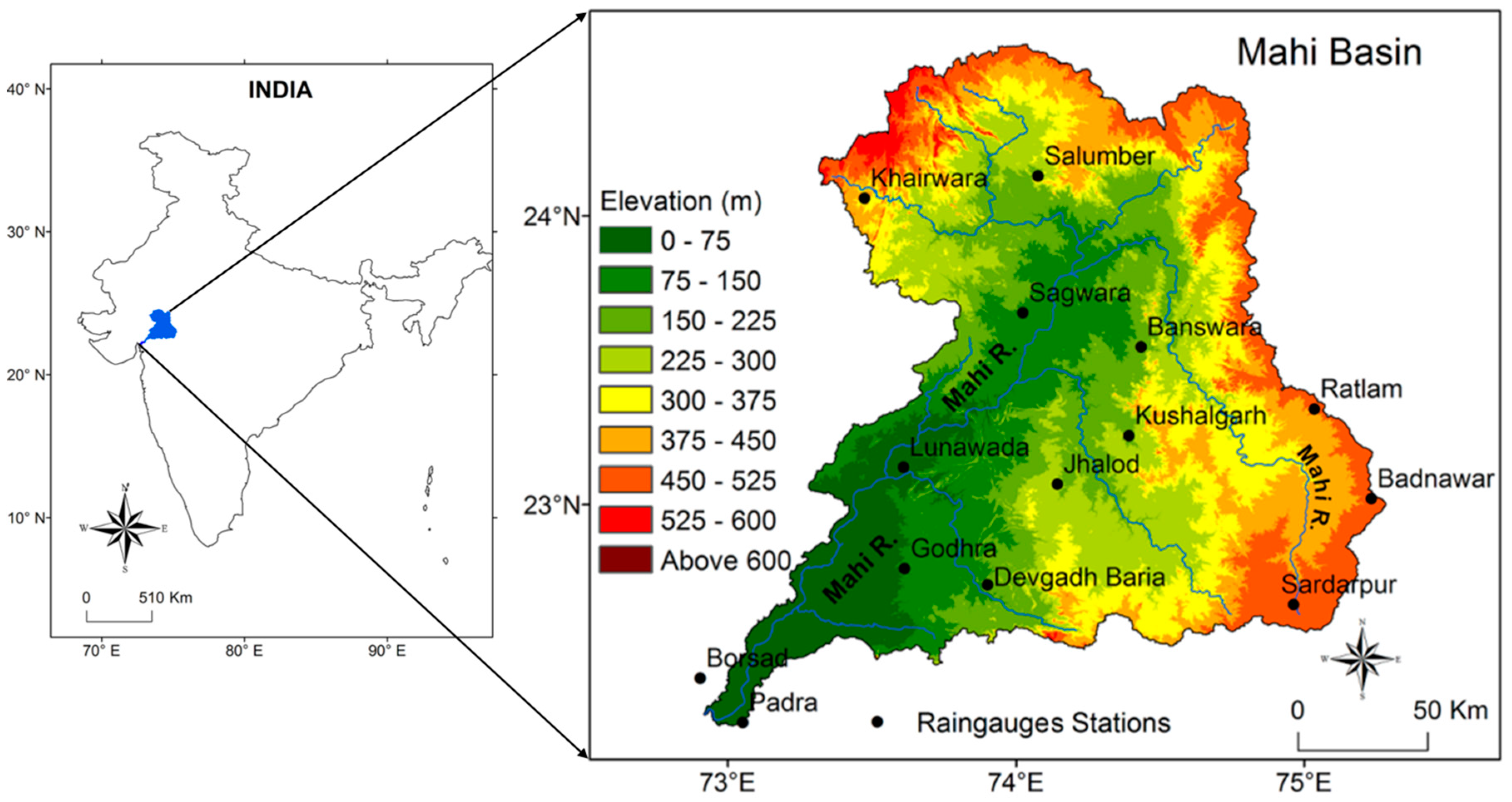
The Mahi River is the third-largest interstate west-flowing river of peninsular India that flows in western India (Figure 1). It originates near the Minda village (Sardarpur) in the Dhar district of Madhya Pradesh at an altitude of 500 m ASL. Its total length is 583 km and meets the Gulf of Khambhat in Gujarat. The Mahi Basin extends between 22°30′ and 24°20′ N latitudes and 73°00′ and 74°20′ E longitudes. The basin covers the areas of Madhya Pradesh, Rajasthan, and Gujarat, with a drainage basin area of 34,842 km2 (Figure 1).
2.2. Data Used
The long-term monthly rainfall data (1901–2012) of 14 rain gauge stations in the Mahi Basin, namely, Badnawar, Banswara, Borsad, Devgadh Baria, Godhra, Jhalod, Khairwara, Kushalgarh, Lunawada, Padra, Ratlam, Sagwara, Salumber, and Sardarpur, were used for the analysis of the rainfall distribution, variability, and trends over the basin (Figure 1). Monthly precipitation records were acquired from the India Meteorological Department (IMD). Moreover, digital elevation model (DEM) data were acquired from the United State Geological Survey (USGS) website (https://earthexplorer.usgs.gov), accessed on 20 August 2019.
2.3. Methodology
The fundamental objective of this study is to comprehend the precipitation distribution, erraticism, and trends in the Mahi Basin on an annual and seasonal scale. Therefore, the long-term rainfall data were categorized into four periods: (i) Monsoon (June-September), (ii) Post-monsoon (October to November), (iii) Winter monsoon (December to February), and (iv) Pre-monsoon (March to May). First, PAST version 4.03 software was used to check the serial autocorrelation in the rainfall time series. The classified data were computed by applying basic quantitative methods (mean, standard deviation (σ), and coefficient of variation (Cv)). Further, the precipitation inconsistency over the Mahi Basin was characterized by a normalized accumulated departure from the mean (NADM) and rainfall departure from the mean (%). The inverse distance weighted (IDW) technique was used for the interpolation of point rainfall values to show a spatial distribution. In addition, digital elevation model (DEM) data were used to show the elevation variation in the basin, to generate the Mahi Basin, Mahi River, and its tributaries. The rainfall trend analysis methodology is as follows.
2.3.1. Coefficient of Variation (CV)
An analysis of the rainfall variation in the Mahi Basin was calculated by Equation (1):
where σ and are the standard deviation and mean rainfall for the annual and seasonal scales.
2.3.2. Mann–Kendall (MK) Test
The Mann–Kendall test was used to identify the significant rainfall trends over the Mahi Basin [61,62]:
where Xj and Xk are the data points for rainfall, n is the length of data j and k (k > j), respectively, and sgn (Xk − Xj) is the sign function as follows:
S approximates a normal distribution with a mean of 0 when n is equal to 10. The variance can be found as given in Equation (4):
where t and Σt are the extent of any given tie indicates and the summation of all ties. The value of is computed using Equation (5):
where Z is the standard normal variate; an increasing (or decreasing) trend can be identified based on the positive (negative) values of Z. A noteworthy trend is observed, and the null hypothesis is rejected when |Z| > Z1 − α/2. All the outcomes were confirmed at α = 0.05 (Z = ±1.96) and α = 0.10 (Z = ±1.66) significance level.
2.3.3. Sen’s Slope (SS)
The Sen’s slope method [63] was applied to study the magnitude of rainfall change by using the following equations:
where Yj and Yk are values in a series at time j and k (j > k), respectively. Qi is Sen’s estimator of slope. If there is a single datum in each time period, then N = n[n − 1]/2, where n is the number of time periods. However, if the number of values in every year are many, then N < n[n − 1]/2, where n is total number of observations. First, N values were ordered from the minimum to maximum. Then, the median of slope () is calculated as follows:
2.3.4. Innovative Trend Analysis (ITA) Method
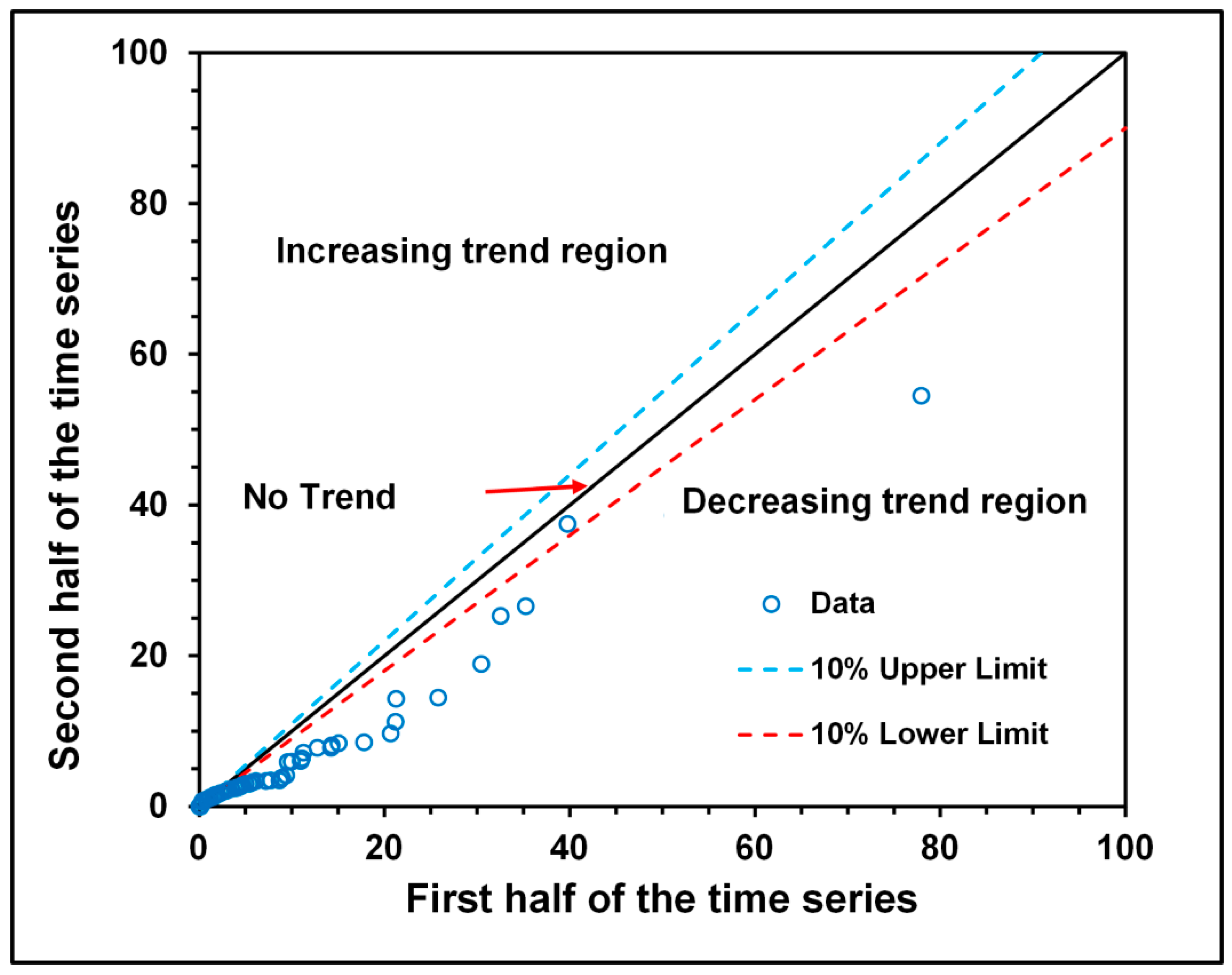
The innovative trend analysis (ITA) method was developed by Şen [64,65] to look at trends in streamflow, temperature, and rainfall. The primary step in ITA is to divide the long-term data into two equal halves, with each half-series’ data being arranged independently in ascending order. An ordinate (X-axis) and an abscissa (Y-axis) are used to plot this subset of data. The diagram in Figure 2 is divided into two equal triangles by the 1:1 (45°) line of no trend. The inclining and declining tendency of the data is depicted in an area above and below the 1:1 line [65]. When all the data points in the scattergram are on or near the 1:1 line, no discernible trend in the time series can be seen.
2.3.5. Pettitt’s Test
The Pettitt’s test (nonparametric test) developed by [66] Pettitt (1979) is useful for change detection. The null hypothesis denotes no change in the time series, whereas the alternative shows a change point exists in the data series. In order to reject the null hypothesis, the test statistic should be larger than the critical value.
If a break occurs in the time series, then the value of Xk reaches the maximum or minimum near the break year k, which is defined as follows:
3. Results and Discussion
3.1. Serial Autocorrelation Analysis
Serial correlation in a hydrometeorological data series can have effect on trend and change-point detection tests [67]. According to numerous studies, the presence of a positive serial correlation in time-series data increases the Type I error in the MK test, and it will lead to an over-rejection of the null hypothesis of no trend [68,69,70]. According to Yue and Wang [1], the presence of serial correlation in hydrometeorological data will affect the results of the MK test. Therefore, to obtain precise outcomes of the trends of rainfall in the Mahi Basin, serial autocorrelation was checked, and the results were represented by correlograms at various time lags for the annual and seasonal rainfall (Figure 3). For various time lags, all correlograms demonstrated that the rainfall values (annual and seasonal) were within the 95% confidence limit (upper and lower). This demonstrates that the time-series data do not exhibit serial autocorrelation. Independence within hydrometeorological time-series data is an important postulation of trend detection tests such as the MK test [67]. Due to the nonexistence of serial autocorrelation, the time-series data were directly used for fundamental statistical analyses, the MK test, and Pettitt’s test of change-point detection for the analysis of rainfall on the annual and seasonal scale in the Mahi Basin. Serinaldi and Kilsby [71] mentioned the significance of the existence and nonexistence of sequential association in hydrometeorological data in the MK and Pettitt’s test.
3.2. Rainfall Characteristics of the Mahi Basin
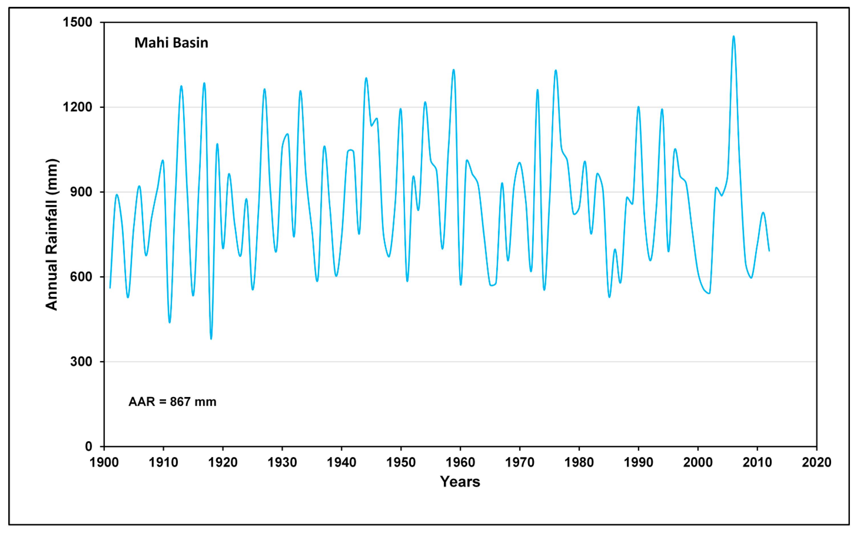
The Mahi Basin receives monsoon rainfall from mid-June with the inception of the southwest monsoon. Figure 4 shows the interannual fluctuations in annual rainfall from 1901 to 2012 with some years (1927, 1959, 1973, 1976, and 2006) of high rainfall linked with a low-pressure system (LPS) [57]. Almost 95% of the rainfall (821 mm) occurs in the monsoon months (Table 1). The monthly rainfall distribution in the Mahi Basin significantly varies in time and space (Figure 5 and Figure 6). July was the wettest (288.7 mm) month across the basin, which accounted for 33.3% of the AAR. About 64.1% of the rainfall in the Mahi Basin occurred in July (33.3%) and August (30.8%) (Table 1). The post-monsoon rainfall (30.3 mm) was more than the winter (6.1 mm) and pre-monsoon rainfall (9.0 mm) in the basin. Table 1 indicates that the mean monthly rainfall (MMR) variation ranged between 56.1% (February) and 14.2% (July) in the Mahi Basin.
3.3. Rainfall Distribution (Annual and Seasonal) over the Mahi Basin
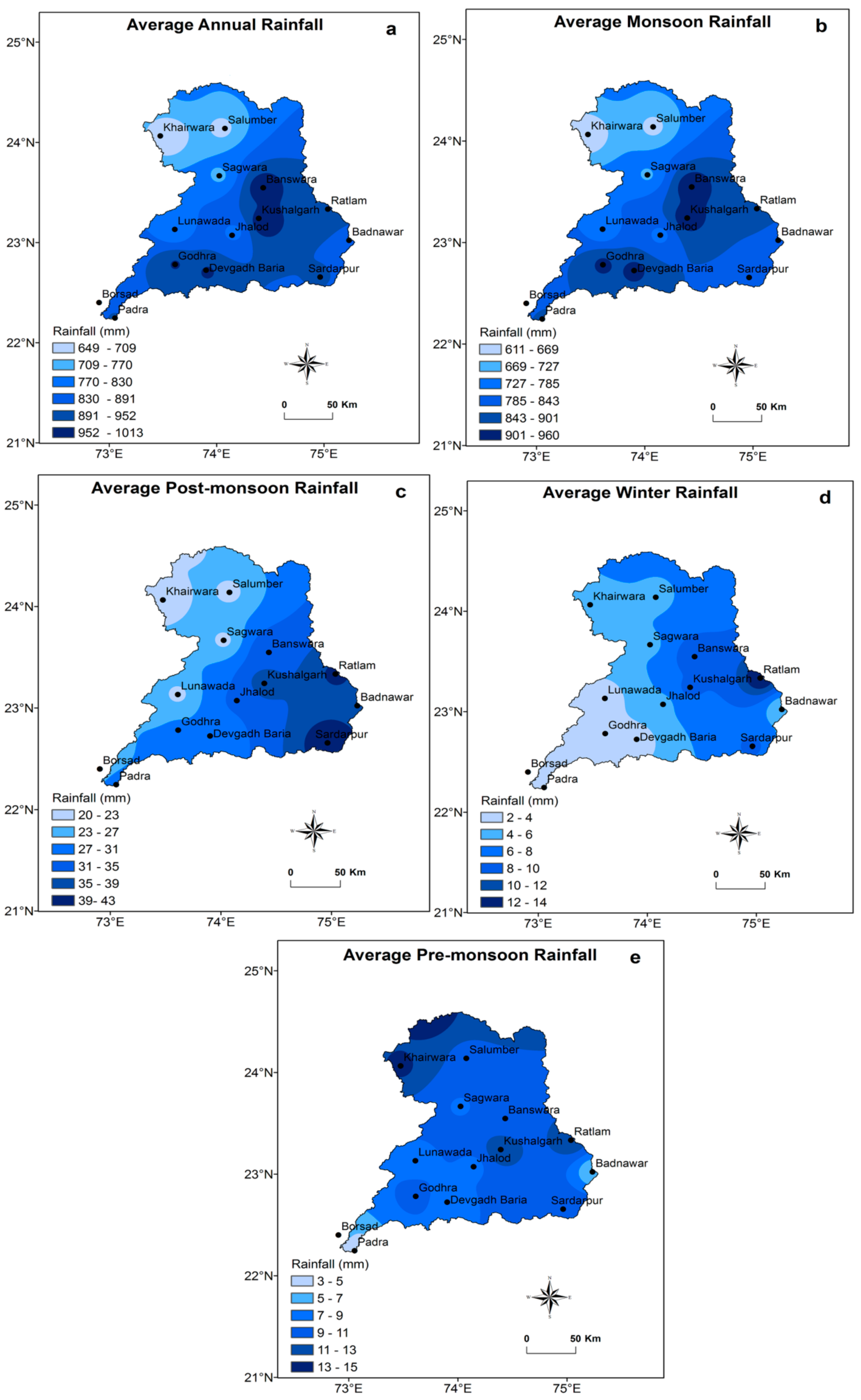
Large oscillations with epochal behavior in the rainfall over the monsoonal regions of the world are the most prominent feature [72]. According to Pawar and Hire [59], low-pressure systems (LPSs) significantly affect the AAR as well as average monsoon rainfall (AMR) of the basin and are a major cause of inundations in the Mahi Basin. Therefore, it is essential to understand the rainfall distribution (annual and seasonal) in the basin (Table 2). The AAR varied between 649 mm (Khairwara) and 1012.8 mm (Banswara), and the AMR ranged between 610.7 mm (Khairwara) and 959.6 mm (Banswara) (Table 2). During the post-monsoon season, Sardarpur received the highest (43.4 mm) rainfall in the basin. All the rain gauge stations received more than 93% of their rainfall in the monsoon season (Table 2). Therefore, it shows that the hydrometeorological features of the basin are considerably associated with monsoon rainfall. Figure 5 and Figure 6 indicate that all the rainfall stations receive the maximum rainfall during the monsoon season (June to September), and rainfall in the non-monsoon season is very negligible.
Figure 7 shows that AAR and AMR decrease from the east and southeast part of the Mahi Basin toward the northwestern and western catchment of the basin. The central and eastern part of the Mahi Basin receives the maximum AAR and AMR (>900 mm), specifically, at Banswara, Devgadh Baria, Godhra, Kushalgarh, and Ratlam (Figure 7a,b). The western catchment area of the basin receives less precipitation in the post-monsoon period due to the early withdrawal of the monsoon (Figure 7c). The northern and northwestern catchment of the Mahi Basin receives the maximum precipitation in the winter and pre-monsoon months due to the effect of western disturbances (Figure 7d,e). Dimri and Mohanty [73] noted the features of the western disturbances (WDs) over the western Himalayas in 2009.
3.4. NADM and Rainfall Departure from the Mean
The rainfall disparity on the annual and seasonal scales is one of the characteristics of the monsoon [74]. The long-term variation in monsoon rainfall is very well understood by the NADM. It is one of the most effective and frequently applied quantitative methods and can resolve successive properties contained by long-term data [75,76,77,78]. Normally, monsoon rainfall shows an epochal nature, alternating between 30 years of dry and wet monsoons [79]. According to Joseph [80,81], tropical disturbances originate above the Bay of Bengal and move in the direction of west and northwest and have a significant impact on the epochal behavior of the monsoon. The NADM graph of the Mahi Basin shows a period of below-average rainfall from 1901 to 1930 and above-average rainfall between 1930 and 1990, followed by a period of fluctuating conditions of the annual and monsoon rainfall (Figure 8a,b). Kripalani et al. [82] also detected random oscillations in annual rainfall and the epochal behavior of above-average and below-average rainfall for decadal rainfall. The maximum positive departure from the mean in the annual and monsoon rainfall represents wet years associated with major floods in the Mahi Basin, such as 1927, 1952, 1959, 1973, 1976, and 2006 [59]. The percent departure from mean rainfall shows a remarkable negative departure from the AAR and AMR during 1901–1930 (Figure 8a,b). The maximum positive departure in annual and monsoon rainfall was associated with LPSs and floods in the basin [59]. Post-monsoon rainfall showed the maximum years of the negative departure of rainfall with notable phases of dry periods (Figure 8c). The winter rainfall shows some remarkable years of the maximum positive departure from the mean rainfall (Figure 8d). Further, Figure 8e shows that pre-monsoon rainfall was recurrently below the long-term average of the pre-monsoon rainfall of the basin.
3.5. Rainfall Varaiation over the Mahi Basin
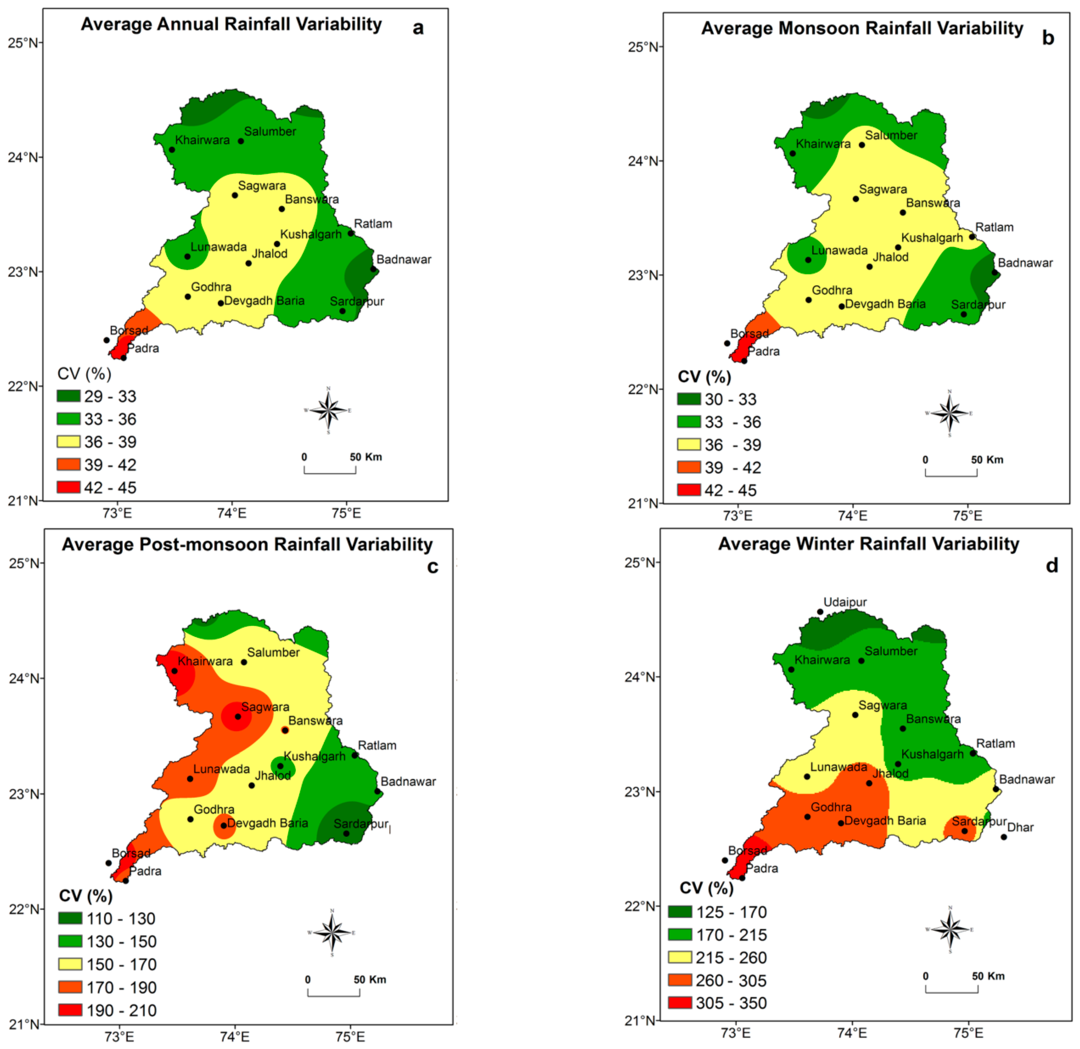
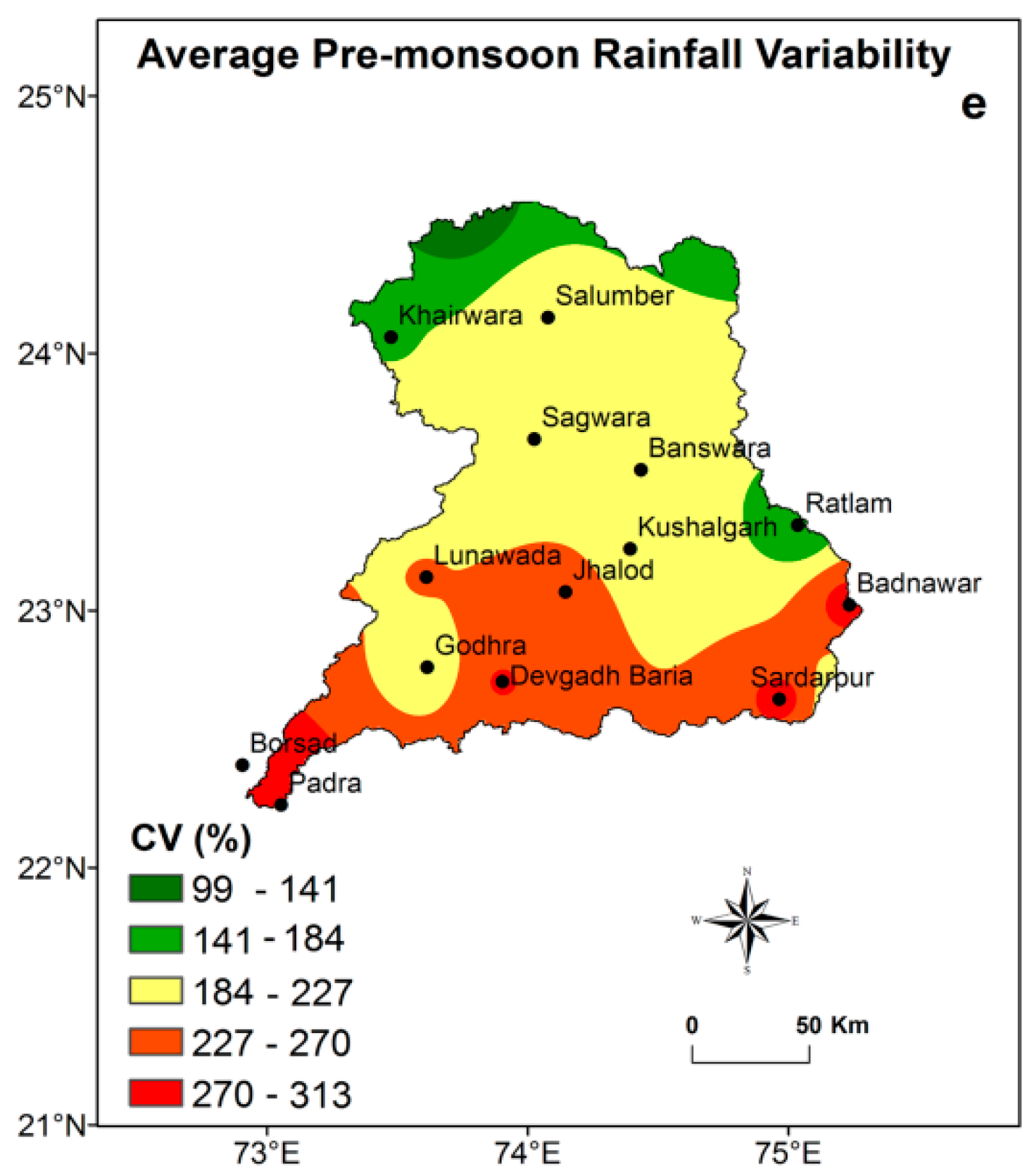
The AAR and AMR of the Mahi Basin did not show significant variations in rainfall (Figure 9a,b). However, rainfall variations are remarkable in the non-monsoon season (Figure 9c–e). The annual and seasonal variations increase from the eastern Mahi Basin toward the west (Figure 9a–e). The highest variations in the AAR and AMR were observed for the Padra station (Figure 9a,b). The lowest variability in the AAR and AMR was reported for the Badnawar station (Figure 9a,b). Figure 9c indicates the average post-monsoon rainfall (APMR) variability ranges between 110% (Sardarpur) and 210% (Borsad). Moreover, the AWR variability ranges between 125% and 350% (Figure 9d). The highest average pre-monsoon rainfall variability (313%) was noticed for the Padra station (Figure 9e). The winter and pre-monsoon rainfall show higher variability in the Mahi Basin (Figure 9d,e). The interannual and interseasonal dissimilarity in rainfall is a significant characteristic of the southwest monsoon [83]. Jhajharia et al. [84] reported a greater variability in rainy days during the non-monsoon season than the monsoon. Guhathakurta and Saji [85] also emphasized that the examination of rainfall variability has great significance for better water resource planning, as well as flood and drought disaster management.
3.6. Rainfall Trend and Magnitude Change in the Mahi Basin
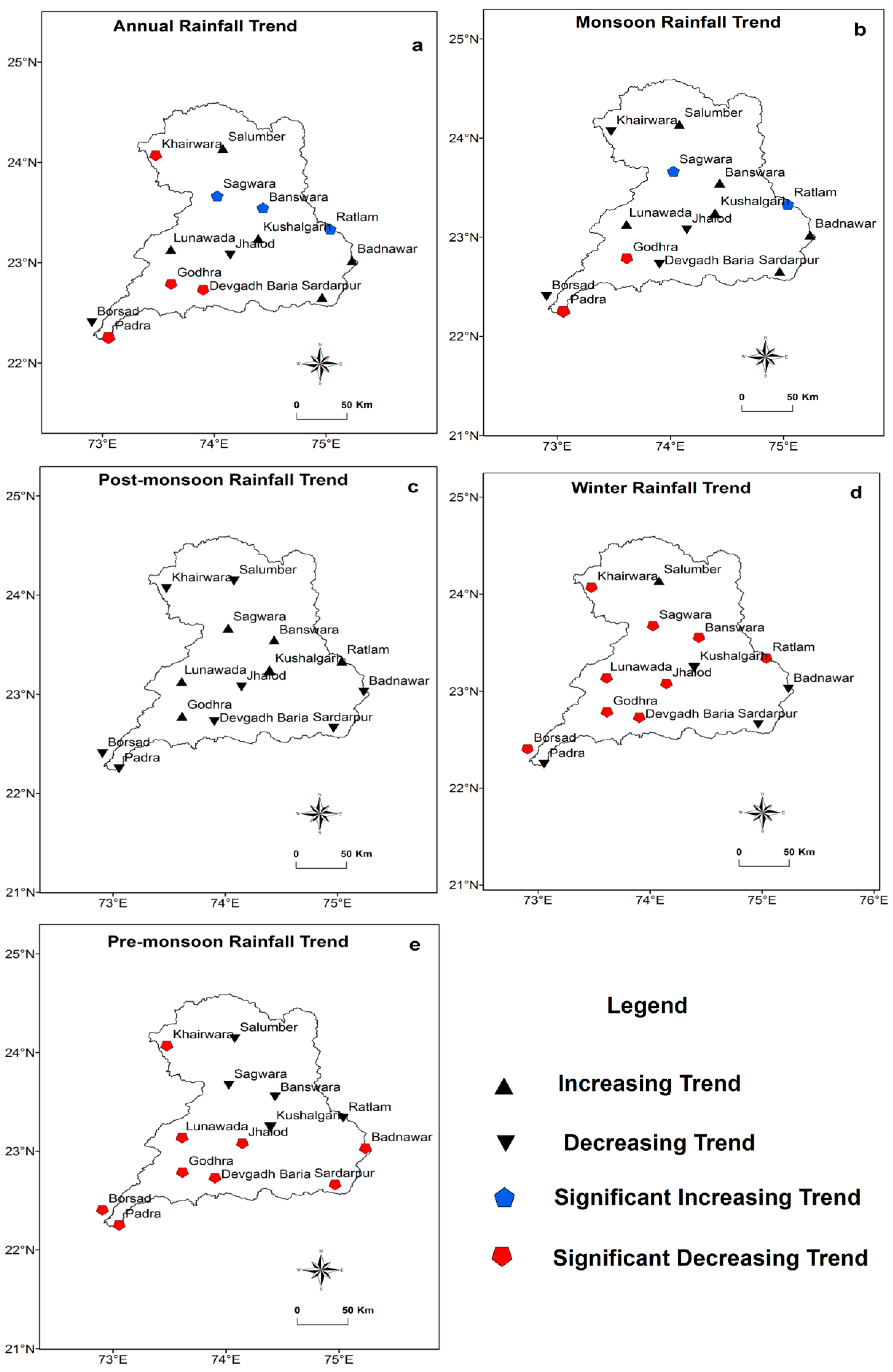
A significant increasing trend of annual rainfall was noted for the Banswara, Ratlam, and Sagwara stations, whereas the Devgadh Baria, Godhra, Khairwara, and Padra stations denoted a significant decreasing rainfall trend on the annual scale (Table 3; Figure 10a). The Godhra station showed a substantial decrease in monsoon rainfall from 1901 to 2012 (1.89 mm/y). Conversely, Ratlam and Sagwara denoted a noteworthy increasing tendency (1.5 mm/y) in monsoon rain from 1901 to 2012 (Table 3; Figure 10b). The post-monsoon rainfall does not exhibit a statistically important decreasing or increasing trend in the Mahi Basin (Table 3; Figure 10c). A noteworthy declining trend of winter precipitation was detected for nine stations, excepting Badnawar, Kushalgarh, Padra, Salumber, and Sardarpur (Table 3; Figure 10d). A significant decrease in pre-monsoon rain was identified for the Badnawar, Borsad, Devgadh Baria, Godhra, Jhalod, Khairwara, Lunawada, Padra, and Sardarpur stations (Table 3; Figure 10e). On the basin scale, a substantial declining tendency was observed for the winter (0.02 mm/y) and pre-monsoon rainfall (0.04 mm/y) during 1901–2012 (Table 3). The annual and monsoon rainfall neither displayed a major increasing nor decreasing tendency on the basin scale. Likewise, Kumar and Jain [30] mentioned that out of 22 river basins in India under investigation, only 2 basins showed noteworthy trends, and the rest of the basins neither indicated an increase nor decrease in annual and seasonal rainfall significantly. Nevertheless, Mooley and Parthasarathy [76] and Thapliyal and Kulshreshtha [24] notified that there is no remarkable positive or negative trend in mean annual rain over India. Therefore, it is concluded that the rainfall trend (increasing or decreasing) was observed in certain pockets of India in the non-monsoon period [25]. This declining trend in seasonal rainfall could be decreasing the frequency of WDs over the northwestern part of India [86]. Moreover, Shekhar et al. [87] observed a decrease in winter rainfall in the Western Himalayan Region (WHR).
Furthermore, the rainfall trend over the Mahi Basin was denoted by ITA graphs (Figure 11a–e). The ITA plots for the annual, monsoon, and post-monsoon rainfall represent that almost all the data points are either on the 1:1 line (no trend) or fall between the 10% upper and lower limits (Figure 11a–c). The ITA graphs obtained for winter and pre-monsoon rainfall show that all the data points are below the 10% lower limit (11d–e). Therefore, it is specified that winter and pre-monsoon rain in the Mahi Basin have significantly declined in the last 112 years. On the basin scale, the comparative rainfall trend analyses of the MK and ITA indicated insignificant increasing or decreasing trends in the annual and monsoon rainfall.
However, there are some critics of the usage of the ITA method for determining climatic trends [88]. The research presented here is not built on the ITA method but on the often-used MK test. Understanding these critics of the ITA method, the results from the MK test and Sen’s slope estimator test were compared against the ITA method.
3.7. Analysis of Change-Point Detection Tests of Rainfall
Pettitt’s test of change-point detection was used to identify the existence of changes in the annual and seasonal rainfall series from 1901 to 2012 (Table 4). The analysis of change-point detection showed that all stations in the Mahi Basin under investigation denoted similar years of shift in annual and monsoon rainfall except Sagwara (Table 4). It strongly suggested that changes (increasing or decreasing) in the monsoon rainfall are eventually reflected in the annual rainfall. Therefore, it is specified that the Mahi Basin is influenced by monsoon rainfall. There are notable variations in years of post-monsoon, winter, and pre-monsoon rainfall from 1901–2012 (Table 4). In addition, annual and seasonal rainfall shifts on the basin scale are represented in Figure 12a–e. On the basin scale, an annual and monsoon rainfall shift was noted after 1926 (Figure 12a,b). According to Pawar et al. [57,59], the shift in the annual and monsoon rainfall of the basin might be influenced by low-pressure systems that affect the rainfall of the Mahi Basin [57,59]. In the case of the post-monsoon season, a shift in rainfall pattern was observed after 1953 (Figure 12c). Nevertheless, the winter and pre-monsoon seasons denoted shifts in rainfall after 1982 and 1933, respectively (Figure 12d,e).
4. Conclusions
Spatiotemporal rainfall analysis showed that the central Mahi Basin receives the maximum rainfall (>900 mm) compared to other parts of the basin. Moreover, winter and pre-monsoon rain spells were observed in the northern and northwestern catchments of the basin. However, the seasonal rain of the basin varied between 26.8% (monsoon) and 142.1% (pre-monsoon). The NADM showed a period of below-average rainfall from 1901 to 1930 and above-average rainfall between 1930 and 1990, followed by a period of fluctuating conditions. The high rainfall variability was observed throughout the post-monsoon, winter, and pre-monsoon seasons. The rainfall trend analysis revealed that annual, monsoon, and post-monsoon rainfall do not show statistically significant decreasing or increasing trends on the basin scale. Nevertheless, a statistically significant declining trend was observed for winter and pre-monsoon rainfall in the Mahi Basin. A noteworthy reduction in annual and monsoon rainfall was observed for Godhra, while Ratlam and Sagwara showed a remarkable rise (1.5 mm/yr.) in monsoon and annual rain (1.83 mm/yr. and 1.49 mm/yr.) from 1901 to 2012. Likewise, 9 stations out of 14 showed a significant decline in winter and pre-monsoon rainfall. The MK test and ITA analyses show that annual, seasonal, and post-monsoon rainfall did not exhibit a substantial rise or fall on the basin scale. A change-point detection showed that after 1926, annual and monsoon rainfall in the Mahi basin shifted (increased). However, there is no significant increase in the annual and monsoon rainfall of the basin. Therefore, it is concluded that rainfall in the Mahi Basin is steady.
Author Contributions
Conceptualization, U.P. and P.H.; methodology, U.P.; software, U.P.; validation, U.P., P.H. and M.B.G.; formal analysis, U.P.; investigation, U.P.; resources, P.H.; data curation, U.P.; writing—original draft preparation, U.P. and P.H.; writing—review and editing, M.B.G. and U.R.; visualization, U.P.; supervision, P.H. and U.R.; project administration, U.P.; funding acquisition, U.P., P.H. and U.R. All authors have read and agreed to the published version of the manuscript.
Funding
The authors are extremely grateful to the Science and Engineering Research Board (SERB), Department of Science and Technology (DST), Government of India, Project Number: EMR/2016/002590, dated 21 February 2017, for providing financial support to carry out this research work.
Data Availability Statement
Data used in this manuscript can be requested for research purposes from the corresponding authors.
Acknowledgments
The authors are very thankful to the India Meteorological Department (IMD), Pune, for providing the rainfall data.
Conflicts of Interest
The authors declare no conflict of interest.
References
- Yue, S.; Wang, C. The Mann-Kendall Test Modified by Effective Sample Size to Detect Trend in Serially Correlated Hydrological Series. Water Resour. Manag. 2004, 18, 201–218. [Google Scholar] [CrossRef]
- Hui-Mean, F.; Yusop, Z.; Yusof, F. Drought analysis and water resource availability using standardised precipitation evapotranspiration index. Atmos. Res. 2018, 201, 102–115. [Google Scholar] [CrossRef]
- Chiew, F.H.S.; McMahon, T.A. Detection of trend or change in annual flow of Australian rivers. Int. J. Climatol. 1993, 13, 643–653. [Google Scholar] [CrossRef]
- Yu, Y.S.; Zou, S.; Whittemore, D. Non-parametric trend analysis of water quality data of rivers in Kansas. J. Hydrol. 1993, 150, 61–80. [Google Scholar] [CrossRef]
- Haigh, M.J. Sustainable management of headwater resources: The Nairobi headwater declaration (2002) and beyond. Asian J. Water Environ. Pollut. 2004, 1, 17–28. [Google Scholar]
- Cannarozzo, M.; Noto, L.V.; Viola, F. Spatial distribution of rainfall trends in Sicily (1921–2000). Phys. Chem. Earth 2006, 31, 1201–1211. [Google Scholar] [CrossRef]
- Goswami, B.N.; Venugopal, V.; Sengupta, D.; Madhusoodanan, M.S.; Xavier, P.K. Increasing Trend of Extreme Rain Events over India in a Warming Environment. Science 2006, 314, 1442–1445. [Google Scholar] [CrossRef] [Green Version]
- Zolina, O.; Simmer, C.; Gulev, S.; Kollet, S. Changing structure of European precipitation: Longer wet periods leading to more abundant rainfalls. Geophys. Res. Lett. 2010, 37, 460–472. [Google Scholar] [CrossRef]
- Kyoung, M.; Kim, H.; Sivakumar, B.; Singh, V.; Ahn, K. Dynamic characteristics of monthly rainfall in the Korean Peninsula under climate change. Stoch. Environ. Res. Risk Assess. 2011, 25, 613–625. [Google Scholar] [CrossRef]
- World Meteorological Organisation. Detecting trend and other changes in hydrological data. In World Climate Program-Water; Kundzewicz, Z.W., Robson, A., Eds.; WMO/UNESCO, WCDMP-45, WMO/TD-No.1013; World Meteorological Organisation: Geneva, Switzerland, 2000. [Google Scholar]
- Karl, T.R.; Knight, R.W. Secular trends of precipitation amount, frequency, and intensity in the United States. Bull. Am. Meteorol. Soc. 1998, 79, 231–241. [Google Scholar] [CrossRef]
- Partal, T.; Kahya, E. Trend analysis in Turkish precipitation data. Hydrol. Process. 2006, 20, 2011–2026. [Google Scholar] [CrossRef]
- Zin, W.Z.W.; Jamaludin, S.; Deni, S.M.; Jemain, A.A. Recent changes in extreme rainfall events in Peninsular Malaysia: 1971–2005. Theor. Appl. Climatol. 2010, 99, 303–314. [Google Scholar] [CrossRef]
- Gocic, M.; Trajkovic, S. Analysis of changes in meteorological variables using Mann-Kendall and Sen’s slope estimator statistical tests in Serbia. Glob. Planet. Chang. 2013, 100, 172–182. [Google Scholar] [CrossRef]
- Kamruzzaman, M.; Beecham, S.; Metcalfe, A.V. Estimation of trends in rainfall extremes with mixed effects models. Atmos. Res. 2016, 168, 24–32. [Google Scholar] [CrossRef]
- Santos, C.A.G.; Morais, B.S. Identification of precipitation zones within São Francisco River basin (Brazil) by global wavelet power spectra. Hydrol. Sci. J. 2013, 58, 789–796. [Google Scholar] [CrossRef]
- Xu, Y.; Xu, Y.; Wang, Y.; Wu, L.; Li, G.; Song, S. Spatial and temporal trends of reference crop evapotranspiration and its influential variables in Yangtze River Delta, eastern China. Theor. Appl. Climatol. 2016, 130, 945–958. [Google Scholar] [CrossRef]
- Dore, M.H.I. Climate change and changes in global precipitation patterns: What do we know? Environ. Int. 2005, 31, 1167–1181. [Google Scholar] [CrossRef]
- Maidment, R.I.; Allan, R.P.; Black, E. Recent observed and simulated changes in precipitation over Africa. Geophys. Res. Lett. 2015, 42, 8155–8164. [Google Scholar] [CrossRef]
- Wang, B.; Bao, Q.; Hoskins, B.; Wu, G.; Liu, Y. Tibetan Plateau warming and precipitation changes in East Asia. Geophys. Res. Lett. 2008, 35, L14702. [Google Scholar] [CrossRef] [Green Version]
- Turner, A.G.; Annamalai, H. Climate change and the South Asian summer monsoon. Nat. Clim. Chang. 2012, 2, 587–595. [Google Scholar] [CrossRef]
- Liu, Q.; Yang, Z.; Cui, B. Spatial and temporal variability of annual precipitation during 1961–2006 in Yellow River Basin, China. J. Hydrol. 2008, 361, 330–338. [Google Scholar] [CrossRef]
- Perera, A.; Mudannayake, S.D.; Azamathulla, H.M.; Rathnayake, U. Recent climatic trends in Trinidad and Tobago, West Indies. Asia-Pac. J. Sci. Technol. 2020, 25, 1–11. [Google Scholar]
- Thapliyal, V.; Kulshrestha, S.M. Climate changes and trends over India. Mausam 1991, 42, 333–338. [Google Scholar] [CrossRef]
- Ray, K.C.S.; Srivastava, A.K. Is there any change in extreme events like heavy rainfall? Curr. Sci. 2000, 79, 155–158. [Google Scholar]
- Sharma, K.P.; Vorosmarty, C.J.; Moore, I.B. Sensitivity of the Himalayan hydrology to landuse and climatic changes. Clim. Chang. 2000, 47, 117–139. [Google Scholar] [CrossRef]
- Bharath, A.; Maddamsetty, R.; Manjunatha, M.; Ramesh, T.V. Spatiotemporal Rainfall Variability and Trend Analysis of Shimsha River Basin, India. Environ. Sci. Pollut. Res. 2023, 1–20. [Google Scholar] [CrossRef]
- Singh, P.; Kumar, V.; Thomas, T.; Arora, M. Changes in rainfall and relative humidity in different river basins in the north-west and central India. Hydrol. Process. 2008, 22, 2982–2992. [Google Scholar] [CrossRef]
- Mirza, M.Q.; Warrick, R.A.; Ericksen, N.J.; Kenny, G.J. Trends and persistence in precipitation in Ganges, Brahmaputra and Meghna River basins. Hydrol. Sci. J. 1998, 43, 845–858. [Google Scholar] [CrossRef]
- Kumar, V.; Jain, S.K. Trends in rainfall amount and number of rainy days in river basins of India (1951–2004). Hydrol. Res. 2011, 42, 290–306. [Google Scholar] [CrossRef]
- Pandey, B.K.; Khare, D. Identification of trend in long term precipitation and reference evapotranspiration over Narmada River basin (India). Glob. Planet. Chang. 2017, 161, 172–182. [Google Scholar] [CrossRef]
- Sharma, P.J.; Loliyana, V.D.; Resmi, S.R.; Timbadiya, P.V.; Patel, P.L. Spatiotemporal trends in extreme rainfall and temperature indices over Upper Tapi Basin, India. Theor. Appl. Climatol. 2018, 134, 1329–1354. [Google Scholar] [CrossRef]
- Hamilton, J.P.; Whitelaw, G.S.; Fenech, A. Mean annual temperature, and annual precipitation trends at Canadian biosphere reserves. Environ. Monit. Assess. 2001, 67, 239–275. [Google Scholar] [CrossRef] [PubMed]
- Dinpashoh, Y.; Mirabbasi, R.; Jhajharia, D.; Abianeh, H.Z.; Mostafaeipour, A. Effect of short-term and long-term persistence on identification of temporal trends. J. Hydrol. Eng. 2014, 19, 617–625. [Google Scholar] [CrossRef]
- Burn, D.H. Hydrologic effects of climatic change in west-central Canada. J. Hydrol. 1994, 160, 53–70. [Google Scholar] [CrossRef]
- Lettenmaier, D.P.; Wood, E.F.; Wallis, J.R. Hydro-climatological trends in the continental United States, 1948–1988. J. Clim. 1994, 7, 586–607. [Google Scholar] [CrossRef]
- Douglas, E.M.; Vogel, R.M.; Kroll, C.N. Trends in floods and low flows in the United States: Impact of spatial correlation. J. Hydrol. 2000, 240, 90–105. [Google Scholar] [CrossRef]
- Hire, P.S. Geomorphic and Hydrologic Studies of Floods in the Tapi Basin. Ph.D. Thesis, University of Pune, Pune, India, 2000. [Google Scholar]
- Miller, W.P.; Piechota, T.C. Regional analysis of trend and step changes observed in hydroclimatic variables around the Colorado River Basin. J. Hydrometeorol. 2008, 9, 1020–1034. [Google Scholar] [CrossRef] [Green Version]
- Ngongondo, C.; Xu, C.Y.; Gottschalk, L.; Alemaw, B.F. Evaluation of spatial and temporal characteristics of rainfall in Malawi: A case of data scarce region. Theor. Appl. Climatol. 2011, 106, 79–93. [Google Scholar] [CrossRef] [Green Version]
- Barua, S.; Muttil, N.; Ng, A.W.M.; Perera, B.J.C. Rainfall trend and its implications for water resource management within the Yarra River catchment, Australia. Hydrol. Process. 2013, 27, 1727–1738. [Google Scholar] [CrossRef] [Green Version]
- Taxak, A.K.; Murumkar, A.R.; Arya, D.S. Long term spatial and temporal rainfall trends and homogeneity analysis in Wainganga basin, Central India. Weather Clim. Extrem. 2014, 4, 50–61. [Google Scholar] [CrossRef] [Green Version]
- Prakash, S.; Sathiyamoorthy, V.; Mahesh, C.; Gairola, R.M. An evaluation of high-resolution multi-satellite rainfall products over the Indian monsoon region. Int. J. Remote Sens. 2014, 35, 3018–3035. [Google Scholar] [CrossRef]
- Bharti, V.; Singh, C. Evaluation of error in TRMM 3B42V7 precipitation estimates over the Himalayan region. J. Geophys. Res. Atmos. 2015, 120, 12458–12473. [Google Scholar] [CrossRef]
- Hire, P.S.; Patil, A.D. Detection of variations in the annual rainfall of the Par Basin using non-parametric Mann-Kendall test. Curr. Glob. Rev. 2018, 1, 103–106. [Google Scholar]
- Malik, A.; Kumar, A.; Guhathakurta, P.; Kisi, O. Spatial-temporal trend analysis of seasonal and annual rainfall (1966–2015) using innovative trend analysis method with significance test. Arab. J. Geosci. 2019, 12, 328. [Google Scholar] [CrossRef]
- Pawar, U.; Rathnayake, U. Spatiotemporal rainfall variability and trend analysis over Mahaweli Basin, Sri Lanka. Arab. J. Geosci. 2022, 15, 370. [Google Scholar] [CrossRef]
- Pawar, U. Rainfall distribution and trends over the semi-arid Marathwada region of Maharashtra, India. Arab. J. Geosci. 2022, 15, 1738. [Google Scholar] [CrossRef]
- Kamal, N.; Pachauri, S. Mann-Kendall Test—A Novel Approach for Statistical Trend Analysis. IJCTT 2018, 63, 18–21. [Google Scholar] [CrossRef]
- Davey, C.A.; Sr Pielke, R.A. Microclimate exposures of surface-based weather stations: Implications for the assessment of long-term temperature trends. Bull. Am. Meteorol. Soc. 2005, 86, 497–504. [Google Scholar]
- Maity, R.; Kumar, D.N.; Nanjundiah, R.S. Review of hydroclimatic teleconnection between hydrologic variables and large-scale atmospheric circulation patterns with Indian perspective. ISH J. Hydraul. Eng. 2007, 13, 77–92. [Google Scholar] [CrossRef]
- Varikoden, H.; Revadekar, J.V.; Kuttippurath, J.; Babu, C.A. Contrasting trends in southwest monsoon rainfall over the Western Ghats region of India. Clim. Dyn. 2019, 52, 4557–4566. [Google Scholar] [CrossRef]
- Malik, A.; Kumar, A. Spatio-temporal trend analysis of rainfall using parametric and non-parametric tests: Case study in Uttarakhand, India. Theor. Appl. Climatol. 2020, 140, 183–207. [Google Scholar] [CrossRef]
- Bhattacharyya, S.; Sreekesh, S.; King, A. Characteristics of extreme rainfall in different gridded datasets over India during 1983–2015. Atmos. Res. 2022, 267, 105930. [Google Scholar] [CrossRef]
- Patakamuri, S.K.; Muthiah, K.; Sridhar, V. Long-Term homogeneity, trend, and change point analysis of rainfall in the arid district of ananthapuramu, Andhra Pradesh State, India. Water 2020, 12, 211. [Google Scholar] [CrossRef] [Green Version]
- Singh, R.; Sah, S.; Das, B.; Vishnoi, L.; Pathak, H. Spatio-temporal trends and variability of rainfall in Maharashtra, India: Analysis of 118 years. Theor. Appl. Climatol. 2021, 143, 883–900. [Google Scholar] [CrossRef]
- Pawar, U.; Hire, P.; Sarukkalige, R.; Rathnayake, U. Hydro-Meteorological Characteristics of the 1973 Catastrophic Flood in the Mahi Basin, India. Water 2023, 15, 1648. [Google Scholar] [CrossRef]
- Zampieri, M.; Ceglar, A.; Dentener, F.; Toreti, A. Wheat yield loss attributable to heat waves, drought and water excess at the global, national and subnational scales. Environ. Res. Lett. 2017, 12, 64008. [Google Scholar] [CrossRef]
- Pawar, U.V.; Hire, P.S. Long term fluctuations and global teleconnections in the monsoonal rainfall and associated floods of the Mahi Basin: Western India. Int. J. Sci. Res. Sci. Technol. 2018, 5, 237–242. [Google Scholar]
- Sharma, A.; Sharma, D.; Panda, S.K. Assessment of spatiotemporal trend of precipitation indices and meteorological drought characteristics in the Mahi River basin, India. J. Hydrol. 2022, 605, 127314. [Google Scholar] [CrossRef]
- Mann, H.B. Nonparametric tests against trend. Econom. J. Econom. Soc. 1945, 13, 245–259. [Google Scholar] [CrossRef]
- Kendall, M.G. Rank Correlation Method, 4th ed.; Charles Griffin: London, UK, 1975; p. 202. [Google Scholar]
- Sen, P.K. Estimates of the regression coefficient based on Kendall’s tau. J. Am. Stat. Assoc. 1968, 63, 1379–1389. [Google Scholar] [CrossRef]
- Şen, Z. Innovative trend analysis methodology. J. Hydrol. Eng. 2012, 17, 1042–1046. [Google Scholar] [CrossRef]
- Şen, Z. Innovative trend significance test and applications. Theor. Appl. Climatol. 2017, 127, 939–947. [Google Scholar] [CrossRef]
- Pettitt, A.N. A non-parametric approach to the change-point problem. J. R. Stat. Soc. Ser. C (Appl. Stat.) 1979, 28, 126–135. [Google Scholar] [CrossRef]
- O’Brien, N.L.; Burn, D.H.; Annable, W.K.; Thompson, P.J. Trend detection in the presence of positive and negative serial correlation: A comparison of block maxima and peaks-over-threshold data. Water Resour. Res. 2021, 57, e2020WR028886. [Google Scholar] [CrossRef]
- Storch, V.; Navarra, A. Analysis of Climate Variability: Applications of Statistical Techniques; Springer: Berlin, Germany, 1995; pp. 1–26. [Google Scholar]
- Yue, S.; Pilon, P.; Phinney, B.; Cavadias, G. The influence of autocorrelation on the ability to detect trend in hydrological series. Hydrol. Process. 2002, 16, 1807–1829. [Google Scholar] [CrossRef]
- Wang, F.; Shao, W.; Yu, H.; Kan, G.; He, X.; Zhang, D.; Ren, M.; Wang, G. Re-evaluation of the Power of the Mann-Kendall Test for Detecting Monotonic Trends in Hydrometeorological Time Series. Front. Earth Sci. 2020, 8, 14. [Google Scholar] [CrossRef]
- Serinaldi, F.; Kilsby, C.G. The importance of pre-whitening in change point analysis under persistence. Stoch. Env. Res. Risk Assess. 2016, 30, 763–777. [Google Scholar] [CrossRef] [Green Version]
- Parthasarathy, B.; Munot, A.A.; Kothawale, D.R. All-India monthly and seasonal rainfall series 1871–1993. Theor. Appl. Climatol. 1994, 49, 217–224. [Google Scholar] [CrossRef]
- Dimri, A.P.; Mohanty, U.C. Simulation of mesoscale features associated with intense western disturbances over western Himalayas. Meteorol. Appl. 2009, 16, 289–308. [Google Scholar] [CrossRef]
- Pawar, U.V. An Analytical Study of Geomorphological, Hydrological, and Meteorological Characteristics of Floods in the Mahi River Basin: Western India. Ph.D. Thesis, Tilak Maharashtra Vidyapeeth, Pune, India, 2019. [Google Scholar]
- Riehl, H.; El-Bakry, M.; Meitin, J. Nile River discharge. Mon. Weather Rev. 1979, 107, 1546–1553. [Google Scholar] [CrossRef]
- Mooley, D.A.; Parthasarthy, B. Fluctuation of all-India summer monsoon rainfall during 1871–1978. Clim. Chang. 1984, 6, 287–301. [Google Scholar] [CrossRef]
- Probst, J.I.; Tardy, Y. Long range stream flow and world continental runoff fluctuations since the beginning of this century. J. Hydrol. 1987, 94, 289–311. [Google Scholar] [CrossRef]
- Kale, V.S. Long-period fluctuations in Monsoon floods in the Deccan Peninsula, India. J. Geol. Soc. India 1999, 53, 5–15. [Google Scholar]
- Patil, A.D.; Hire, P.S. Flood hydrometeorological situations associated with monsoon floods on the Par River in western India. Mausam 2020, 71, 687–698. [Google Scholar]
- Joseph, P.V. Climate change in monsoon and cyclones. In Proceedings of the IIYTM Symposium on Monsoons, Pune, India, 8–10 September 1976; pp. 378–387. [Google Scholar]
- Joseph, P.V. Sub-tropical westerlies in relation to large scale failure of Indian monsoon. Indian J. Meteorol. Hydrol. Geophys. 1978, 29, 412–418. [Google Scholar] [CrossRef]
- Kripalani, R.H.; Kulkarni, A.; Sabade, S.S. Indian Monsoon variability in a global warming scenario. Nat. Hazards 2003, 29, 189–206. [Google Scholar] [CrossRef]
- Gadgil, S.; Rajeevan, M.; Francis, P.A. Monsoon variability: Links to major oscillations over the equatorial Pacific and Indian Ocean. Curr. Sci. 2007, 93, 182–194. [Google Scholar]
- Jhajharia, D.; Yadav, B.K.; Maske, S.; Chattopadhyay, S.; Kar, A.K. Identification of trends in rainfall, rainy days and 24 h maximum rainfall over subtropical Assam in Northeast India. C. R. Geosci. 2012, 344, 1–13. [Google Scholar] [CrossRef]
- Guhathakurta, P.; Saji, E. Detecting changes in rainfall pattern and seasonality index vis-à-vis increasing water scarcity in Maharashtra. J. Earth Syst. Sci. 2013, 122, 639–649. [Google Scholar] [CrossRef] [Green Version]
- Das, M.R.; Mukhopadhyay, R.K.; Dandekar, M.M.; Kshirsagar, S.R. Pre-monsoon western disturbances in relation to monsoon rainfall, its advancement over NW India and their trends. Curr. Sci. 2002, 82, 1320–1321. [Google Scholar]
- Shekhar, M.S.; Chand, H.; Kumar, S.; Srinivasan, K.; Ganju, A. Climate-change studies in the western Himalaya. Ann. Glaciol. 2010, 51, 105–112. [Google Scholar] [CrossRef] [Green Version]
- Serinaldi, F.; Chebana, F.; Kilsby, C.G. Dissecting innovative trend analysis. Stoch. Environ. Res. Risk Assess. 2020, 34, 733–754. [Google Scholar] [CrossRef]
Figure 1.
Mahi Basin location and study area map.

Figure 2.
Illustration of the ITA method, Red arrow indicates line of ‘No Trend’.

Figure 3.
Correlogram for rainfall of the Mahi Basin: (a) For Annual; (b) For Monsoon Season; (c) For Post-monsoon Season; (d) For Winter Season; (e) For Pre-monsoon Season.
Figure 3.
Correlogram for rainfall of the Mahi Basin: (a) For Annual; (b) For Monsoon Season; (c) For Post-monsoon Season; (d) For Winter Season; (e) For Pre-monsoon Season.

Figure 4.
Annual rainfall of the Mahi Basin from 1901 to 2012.

Figure 5.
Station wise mean monthly rainfall distribution.

Figure 6.
Spatial distribution of the mean monthly rainfall of the Mahi Basin: (a) For January; (b) For February; (c) For March; (d) For April; (e) For May; (f) For June; (g) For July; (h) For August; (i) For September; (j) For October; (k) For November; (l) For December.
Figure 6.
Spatial distribution of the mean monthly rainfall of the Mahi Basin: (a) For January; (b) For February; (c) For March; (d) For April; (e) For May; (f) For June; (g) For July; (h) For August; (i) For September; (j) For October; (k) For November; (l) For December.

Figure 7.
Average rainfall distribution in the Mahi Basin: (a) For Annual; (b) For Monsoon; (c) For Post-monsoon; (d) For Winter; (e) For Pre-monsoon.
Figure 7.
Average rainfall distribution in the Mahi Basin: (a) For Annual; (b) For Monsoon; (c) For Post-monsoon; (d) For Winter; (e) For Pre-monsoon.

Figure 8.
NADM and rainfall departure from the mean rainfall of the Mahi Basin: (a) For Annual; (b) For Monsoon; (c) For Post-monsoon; (d) For Winter; (e) For Pre-monsoon.
Figure 8.
NADM and rainfall departure from the mean rainfall of the Mahi Basin: (a) For Annual; (b) For Monsoon; (c) For Post-monsoon; (d) For Winter; (e) For Pre-monsoon.

Figure 9.
Rainfall variations in the Mahi Basin: (a) For Annual; (b) For Monsoon; (c) For Post-monsoon; (d) For Winter; (e) For Pre-monsoon.
Figure 9.
Rainfall variations in the Mahi Basin: (a) For Annual; (b) For Monsoon; (c) For Post-monsoon; (d) For Winter; (e) For Pre-monsoon.


Figure 10.
Rainfall trends in the Mahi Basin: (a) For Annual; (b) For Monsoon; (c) For Post-monsoon; (d) For Winter; (e) For Pre-monsoon.
Figure 10.
Rainfall trends in the Mahi Basin: (a) For Annual; (b) For Monsoon; (c) For Post-monsoon; (d) For Winter; (e) For Pre-monsoon.

Figure 11.
Rainfall trends by ITA over the Mahi Basin: (a) For Annual; (b) For Monsoon; (c) For Post-monsoon; (d) For Winter; (e) For Pre-monsoon.
Figure 11.
Rainfall trends by ITA over the Mahi Basin: (a) For Annual; (b) For Monsoon; (c) For Post-monsoon; (d) For Winter; (e) For Pre-monsoon.

Figure 12.
Rainfall change-point detection using Pettitt’s test for rainfall in the Mahi Basin: (a) For Annual; (b) For Monsoon; (c) For Post-monsoon; (d) For Winter; (e) For Pre-monsoon.
Figure 12.
Rainfall change-point detection using Pettitt’s test for rainfall in the Mahi Basin: (a) For Annual; (b) For Monsoon; (c) For Post-monsoon; (d) For Winter; (e) For Pre-monsoon.


Table 1.
Rainfall statistics summary of the Mahi Basin (1901–2012).
| Time | Rainfall (mm) | SD (mm) | Cv (%) | Contribution to Annual Rainfall (%) |
|---|---|---|---|---|
| January | 2.4 | 1.2 | 51.3 | 0.3 |
| February | 1.4 | 0.8 | 56.1 | 0.2 |
| March | 1.6 | 0.7 | 41.1 | 0.2 |
| April | 1.1 | 0.4 | 38.0 | 0.1 |
| May | 5.9 | 2.2 | 37.5 | 0.7 |
| June | 111.7 | 21.2 | 19.0 | 12.9 |
| July | 288.7 | 40.9 | 14.2 | 33.3 |
| August | 267.4 | 38.1 | 14.3 | 30.8 |
| September | 150.6 | 24.9 | 16.6 | 17.4 |
| October | 21.7 | 6.4 | 29.3 | 2.5 |
| November | 8.9 | 2.3 | 25.3 | 1.0 |
| December | 2.3 | 1.0 | 43.3 | 0.3 |
| Monsoon | 821.0 | 220.4 | 26.8 | 94.8 |
| Post-monsoon | 30.3 | 36.2 | 119.6 | 3.5 |
| Winter | 6.1 | 7.8 | 127.2 | 0.7 |
| Pre-monsoon | 9.0 | 12.6 | 142.1 | 1.0 |
| Annual | 867.0 | 221.4 | 25.5 |
Table 2.
Average annual and seasonal rainfall distribution in the Mahi Basin.
| Stations/Basin | AAR | Monsoon | Post-Monsoon | Winter | Pre-Monsoon | Monsoon | Non-Monsoon |
|---|---|---|---|---|---|---|---|
| (mm) | (mm) | (mm) | (mm) | (mm) | % | % | |
| Badnawar | 878.0 | 829.1 | 39.2 | 5.0 | 4.7 | 94.4 | 5.6 |
| Banswara | 1012.8 | 959.6 | 35.2 | 9.1 | 8.9 | 94.7 | 5.3 |
| Borsad | 823.9 | 791.8 | 23.6 | 2.9 | 5.6 | 96.1 | 3.9 |
| Devgadh Baria | 959.0 | 919.5 | 28.2 | 3.7 | 7.5 | 95.9 | 4.1 |
| Godhra | 956.8 | 914.9 | 28.4 | 4.2 | 9.3 | 95.6 | 4.4 |
| Jhalod | 813.8 | 767.6 | 31.8 | 6.4 | 8.0 | 94.3 | 5.7 |
| Khairwara | 649.0 | 610.7 | 20.3 | 5.2 | 12.9 | 94.1 | 5.9 |
| Kushalgarh | 1010.9 | 953.0 | 38.1 | 7.6 | 12.2 | 94.3 | 5.7 |
| Lunawada | 769.8 | 735.4 | 22.7 | 3.9 | 7.9 | 95.5 | 4.5 |
| Padra | 906.5 | 869.2 | 30.4 | 4.1 | 2.8 | 95.8 | 4.2 |
| Ratlam | 943.4 | 879.2 | 39.9 | 12.2 | 12.1 | 93.2 | 6.8 |
| Sagwara | 759.8 | 720.3 | 25.4 | 5.8 | 8.3 | 94.8 | 5.2 |
| Salumber | 691.3 | 652.2 | 22.8 | 6.4 | 10.0 | 94.3 | 5.7 |
| Sardarpur | 904.4 | 842.7 | 43.4 | 7.8 | 10.5 | 93.2 | 6.8 |
| Mahi Basin | 867.0 | 821.0 | 30.3 | 6.1 | 9.0 | 94.8 | 5.2 |
Note: Bold values in the table show the highest AAR and seasonal rainfall.
Table 3.
Summary of the rainfall trend analysis (Mann–Kendall and Sen’s slope).
| SN | Stations | Annual | Monsoon | Post-Monsoon | Winter | Pre-Monsoon | |||||
|---|---|---|---|---|---|---|---|---|---|---|---|
| MK z | SS mm/y | MK z | SS mm/y | MK z | SS mm/y | MK z | SS mm/y | MK z | SS mm/y | ||
| 1 | Badnawar | 1.24 | 1.52 | 1.11 | 1.50 | −0.54 | 0.00 | −0.83 | 0.00 | −2.74 | 0.00 |
| 2 | Banswara | 1.68 | 1.77 | 1.34 | 1.6 | 0.61 | 0.00 | −2.10 | 0.00 | −1.54 | 0.00 |
| 3 | Borsad | −0.45 | −0.67 | −0.68 | −0.58 | −0.86 | 0.00 | −3.59 | 0.00 | −3.60 | 0.00 |
| 4 | D. Baria | −1.65 | −1.63 | −1.22 | −1.37 | −0.41 | 0.00 | −4.22 | 0.00 | −4.65 | 0.00 |
| 5 | Godhra | −1.71 | −1.92 | −1.71 | −1.89 | 0.49 | 0.09 | −4.46 | 0.00 | −3.43 | 0.00 |
| 6 | Jhalod | −0.47 | −0.33 | −0.13 | −0.13 | −0.45 | 0.00 | −4.45 | 0.00 | −4.94 | 0.00 |
| 7 | Khairwara | −1.78 | −1.25 | −1.37 | −1.07 | −0.07 | 0.00 | −4.17 | 0.00 | −2.30 | 0.00 |
| 8 | Kushalgarh | 0.5 | 55 | 0.27 | 0.33 | 1.39 | 0.14 | −1.01 | 0.00 | −0.18 | 0.00 |
| 9 | Lunawada | 0.45 | 0.38 | 0.33 | 0.28 | 1.09 | 0.04 | −2.97 | 0.00 | −2.78 | 0.00 |
| 10 | Padra | −1.88 | −6.11 | −1.64 | −5.04 | −1.13 | −0.25 | −0.58 | 0.00 | −1.99 | 0.00 |
| 11 | Ratlam | 1.88 | 1.83 | 1.86 | 1.56 | 1.31 | 0.01 | −2.34 | −0.01 | −1.61 | −0.05 |
| 12 | Sagwara | 1.75 | 1.41 | 1.68 | 1.50 | 0.10 | 0.00 | −1.72 | 0.0 | −1.49 | 0.00 |
| 13 | Salumber | 0.53 | 0.36 | 0.94 | 1.16 | −0.08 | 0.27 | 0.54 | 0.03 | 0.20 | 0.00 |
| 14 | Sardarpur | 0.06 | 0.07 | 0.20 | 0.25 | −0.26 | 0.00 | −1.25 | 0.00 | −1.93 | 0.00 |
| 15 | Mahi Basin | −0.23 | −0.14 | 0.02 | 0.01 | 0.90 | 0.03 | −2.44 | −0.02 | −2.48 | −0.04 |
Bold values are statistically significant at 0.05%, and bold and italic values are statistically significant at 0.10%.
Table 4.
Summary of the rainfall change-point detection using Pettitt’s test.
| Stations/Basin | Annual Rainfall | Monsoon Rainfall | Post-Monsoon Rainfall | Winter Rainfall | Pre-Monsoon Rainfall | |||||
|---|---|---|---|---|---|---|---|---|---|---|
| Shift | Year | Shift | Year | Shift | Year | Shift | Year | Shift | Year | |
| Badnawar | Yes | 1957 | Yes | 1957 | Yes | 1953 | Yes | 1957 | Yes | 1938 |
| Banswara | Yes | 1940 | Yes | 1940 | Yes | 1972 | Yes | 1982 | Yes | 1943 |
| Borsad | Yes | 1959 | Yes | 1959 | Yes | 1985 | Yes | 1948 | Yes | 1959 |
| D. Baria | Yes | 1962 | Yes | 1962 | Yes | 1963 | Yes | 1955 | Yes | 1947 |
| Godhra | Yes | 1959 | Yes | 1959 | Yes | 1926 | Yes | 1942 | Yes | 1957 |
| Jhalod | Yes | 1984 | Yes | 1984 | Yes | 1988 | Yes | 1968 | Yes | 1967 |
| Khairwara | Yes | 1963 | Yes | 1963 | Yes | 1973 | Yes | 1948 | Yes | 1933 |
| Kushalgarh | Yes | 1926 | Yes | 1926 | Yes | 1953 | Yes | 1997 | Yes | 1916 |
| Lunawada | Yes | 1940 | Yes | 1940 | Yes | 1953 | Yes | 1944 | Yes | 1947 |
| Padra | Yes | 1929 | Yes | 1929 | Yes | 1931 | Yes | 1943 | Yes | 1928 |
| Ratlam | Yes | 1932 | Yes | 1932 | Yes | 1954 | Yes | 1967 | Yes | 1962 |
| Sagwara | Yes | 1964 | Yes | 1978 | Yes | 1964 | Yes | 1974 | Yes | 1936 |
| Salumber | Yes | 1946 | Yes | 1946 | Yes | 1917 | Yes | 1922 | Yes | 1918 |
| Sardarpur | Yes | 1978 | Yes | 1978 | Yes | 1903 | Yes | 1963 | Yes | 1962 |
| Mahi Basin | Yes | 1926 | Yes | 1926 | Yes | 1953 | Yes | 1982 | Yes | 1933 |
Disclaimer/Publisher’s Note: The statements, opinions and data contained in all publications are solely those of the individual author(s) and contributor(s) and not of MDPI and/or the editor(s). MDPI and/or the editor(s) disclaim responsibility for any injury to people or property resulting from any ideas, methods, instructions or products referred to in the content. |
© 2023 by the authors. Licensee MDPI, Basel, Switzerland. This article is an open access article distributed under the terms and conditions of the Creative Commons Attribution (CC BY) license (https://creativecommons.org/licenses/by/4.0/).
Share and Cite
MDPI and ACS Style
Pawar, U.; Hire, P.; Gunathilake, M.B.; Rathnayake, U. Spatiotemporal Rainfall Variability and Trends over the Mahi Basin, India. Climate 2023, 11, 163. https://doi.org/10.3390/cli11080163
AMA Style
Pawar U, Hire P, Gunathilake MB, Rathnayake U. Spatiotemporal Rainfall Variability and Trends over the Mahi Basin, India. Climate. 2023; 11(8):163. https://doi.org/10.3390/cli11080163
Chicago/Turabian StylePawar, Uttam, Pramodkumar Hire, Miyuru B. Gunathilake, and Upaka Rathnayake. 2023. "Spatiotemporal Rainfall Variability and Trends over the Mahi Basin, India" Climate 11, no. 8: 163. https://doi.org/10.3390/cli11080163
Note that from the first issue of 2016, this journal uses article numbers instead of page numbers. See further details here.