Effect of Model Structure and Calibration Algorithm on Discharge Simulation in the Acısu Basin, Turkey

Abstract

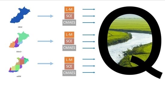
In this study, the Acısu Basin—viz., the headwater of the Gediz Basin—in Turkey, was modelled using three types of hydrological models and three different calibration algorithms. A well-known lumped model (GR4J), a commonly used semi-distributed (SWAT+) model, and a skillful distributed (mHM) hydrological model were built and integrated with the Parameter Estimation Tool (PEST). PEST is a model-independent calibration tool including three algorithms—namely, Levenberg Marquardt (L-M), Shuffled Complex Evolution (SCE), and Covariance Matrix Adoption Evolution Strategy (CMA-ES). The calibration period was 1991–2000, and the validation results were obtained for 2002–2005. The effect of the model structure and calibration algorithm selection on the discharge simulation was evaluated via comparison of nine different model-algorithm combinations. Results have shown that mHM and CMA-ES combination performed the best discharge simulation according to NSE values (calibration: 0.67, validation: 0.60). Although statistically the model results were classified as acceptable, the models mostly missed the peak values in the hydrograph. This problem may be related to the interventions made in 2000–2001 and may be overcome by changing the calibration and validation periods, increasing the number of iterations, or using the naturalized gauge data.

1. Introduction

Hydrological models are used in various areas such as climate models, management of water resources, design of hydraulic structures, and drought/flood prediction. The capabilities of hydrological models are limited by the data and measurement techniques that are used. If the input of model is insufficient, temporal or spatial extrapolation is used with the available data. At the same time, the changes in land use and climate conditions need to be considered in terms of their effects on the hydrologic cycle [1].

Hydrological models, classified in terms of their spatial resolutions, are investigated in this study. These structures are lumped, semi-distributed, and distributed. Lumped models represent the whole basin as a single unit by using the averages of the variables that belong to the basin [2]. Distributed models split the basin into grids and conduct the process for each grid individually with the inputs and state variables that belong to these grids. Semi-distributed models combine the advantages of both lumped and distributed models. Instead of defining the spatial variability as continuous, as the distributed models do, semi-distributed models define the basin as an integration of lumped models. In this way, they require less computational load and smaller data than the distributed models. They also represent the characteristics and heterogeneity of the basin better than lumped models. There are numerous studies in the literature on hydrological modelling in recent decades [3,4,5]. For example, [6] focused on the changes in the Lake Tana Basin, Ethiopia, using different models and their hydrological responses. The researchers built two lumped models (GR4J and IHACRES) and a semi-distributed model (SWAT) for the study area using four major gauged watersheds. The findings of the study showed that the lumped models demonstrated superior discharge simulation performance to SWAT in small catchment, although the situation is reversed in large catchments since SWAT represents the heterogeneity of these catchments. In [7], researchers aimed to test GR4J and SWAT for robustness. Both have undergone calibration and validation studies during climatically diverse time periods. Both exhibit relative robustness despite a greater performance decline for the GR4J model between calibration and validation. Additionally, [8] compared three lumped models’—GR4J, Australian Water Balance Model (AWMB), and Sacramento—discharge performances on the Godavari River Basin, India, considering NSE values of the calibration results. The results of the study showed that the GR4J model is helpful in terms of discharge simulations for the study area. In [9], 15 hydrological models, including GR4J, SWAT, and mHM, were built for Lake Erie, USA, to evaluate the models’ capabilities on hydrological variables such as discharge, evaporation, and soil moisture. The findings of the study demonstrated that the best hydrographs are produced by the mHM model in terms of the resulting NSE values.

Regardless of their classification, the non-measurable parameters of each hydrological model need to be adjusted to represent real basin characteristics. This process is known as calibration [10]. Initially, the calibration process was conducted manually based on expert knowledge. Today, using automatic calibration methods with the advantages of improved technology is more common. These calibration methods avoid subjective interceptions, computation load, and waste of time by using different algorithms and objective functions. Auto-calibration algorithms attain parameter values to optimize objective function value. There are two different types of auto-calibration algorithms, namely, local and global. Local calibration algorithms aim to converge the optimum objective function value based on three main criteria: movement direction of parameters, iteration number, and termination criteria. Local methods that assign gradient-based values to the parameters in their range accept the zero-slope point as the optimum value. This causes possible optimum values to be missed if more than one optimum solution is found. Global methods overcome this problem by approaching the parameter space from all sides. They manipulate parameter values in order to improve the objective function by using deterministic and probabilistic rules [11]. These algorithm types have been used with various hydrological models in several studies. In [12], researchers integrated one local (Levenberg–Marquardt (LM)), and two global (Dynamically Dimensioned Search (DDS) and Shuffled Complex Evolution (SCE)) algorithms with a semi-distributed hydrological model (HEC-HMS) built on various basins in Germany. They used an empirical combination of Nash-Sutcliffe Efficiency (NSE) and volumetric error (VoE) as the objective function for discharge calibration, and they found that DDS is superior to other algorithms in this study’s circumstances with 0.75–0.90 in calibration and 0.57–0.73 in validation. Furthermore, [13] investigated the value of different soil moisture products (The Advanced Microwave Scanning Radiometer on the Earth Observing System (EOS) Aqua satellite (AMSR-E), soil moisture active passive (SMAP), and total water storage anomalies from Gravity Recovery and Climate Experiment (GRACE)) on Hydrologiska Bryåns Vattenbalansavdelning (HBV) by multi-objective calibration (discharge (Q), groundwater (GW), soil moisture (SM)) and soil for each model set-up with Levenberg–Marquardt (LM), shuffled complex evolution (SCE), and covariance matrix adoption evolution strategy (CMAES) algorithms for the Moselle River Basin in Germany and France. The findings of the study demonstrated that the global optimization algorithms (SCE and CMAES) outperformed the local algorithm (LM) after 3000 iterations for each method according to three different objective functions, namely, NSE-Q, NSE-LNQ, and CORR. Additionally, [14] compared the discharge simulation performances resulting from calibration with the SCE and sequential uncertainty fitting algorithm (SUFI2) for the SWAT model to assess the climate change impact for the Upper Coruh Basin in Turkey under regional climate projections (RCP 4.5 and RCP 8.5). The SUFI2 algorithm has 0.67 and 0.62 NSE values for calibration and validation periods, respectively. The SCE algorithm has shown better performance with 0.73 (calibration) and 0.79 (validation) NSE values. There have been many studies on performance comparison of similar and simple models; however, the effect of sophisticated models and global search algorithms on discharge performances in a headwater catchment has not been studied yet. Selection of the model and calibration algorithm is key for discharge simulations in catchment hydrology.

In this study, we integrated three different model structures with three calibration algorithms for the Acısu Basin. We used PEST and ERA5 model inputs. We selected GR4J as the lumped model, SWAT+ as the semi-distributed model, and mHM as the distributed model, and the Levenberg–Marquardt (LM), Shuffled Complex Evolution (SCE), and Covariance Matrix Adoption Evolution Strategy (CMAES) as the calibration algorithms. The resulting discharge values were compared for all combinations. The effect of the model structure and calibration algorithm on discharge performances was evaluated according to these results.

2. Materials and Methods

2.1. Study Area

The Gediz Basin, which is located at the Aegean Region of Turkey, has a surface area of 1,703,586 km². It is one of the 5 largest basins in Turkey. It originates from Murat Mountain in Kutahya. The longest river in the basin is the Gediz River, which ends in the Aegean Sea in İzmir. Including 5 dams, 2 lakes, and 1 hydropower plant, the Gediz Basin is of capital importance in terms of water resources. The water potential of the basin consists of 58.63% potential evapotranspiration loss, 28.22% groundwater recharge, and 13.15% surface flow. The Acısu Basin is a sub-basin of the Gediz Basin, and it has a drainage area of 3256 km² and a height of 890 m. It is located at the headwater of the Gediz Basin with its semi-arid climate. The study area is the drainage area of the stream gauging station 523. The study domain is given in Figure 1.

2.2. Data

In this study, common datasets are defined for each model to evaluate and compare results fairly. So, the three models are driven by ERA5 reanalysis data. Each model requires various data types in different resolutions. Therefore, the daily meteorological input—precipitation (P (mm)), potential evapotranspiration (PET (mm)), and minimum and maximum temperature (T_min (°C), T_max (°C))—obtained from the ERA5 dataset is used by downscaling in line with each model’s resolution. Further, measured P, T_average, T_min, and T_max data, which belong to General Directorate of Meteorology of Turkey (MGM), were used to evaluate the ERA5 data (

Table 1. Monthly and annual data belong to the General Directorate of Meteorology of Turkey and ERA5.

	Total Precipitation (mm)		Average Temperature (°C)		Maximum Temperature (°C)		Minimum Temperature (°C)
	MGM	ERA5	MGM	ERA5	MGM	ERA5	MGM	ERA5
January	69.2	59.7	3.2	3.2	12.8	12.3	−10.6	−9.4
February	62.2	56.1	3.4	3.9	14.4	14.2	−8.9	−9.9
March	60.0	58.6	6.5	7.2	19.2	18.8	−6.5	−5.2
April	63.5	56.6	11.0	11.9	21.5	21.6	−1.2	−0.1
May	43.7	40.2	15.6	16.8	23.3	24.9	4.2	5.2
June	19.8	17.9	19.8	21.4	27.3	28.6	9.9	9.6
July	17.4	10.2	23.3	24.6	30.2	30.8	12.8	15.5
August	12.4	7.6	23.3	24.3	29.7	30.4	15.9	17.3
September	14.7	10.1	19.2	20.0	26.9	28.3	9.4	11.1
October	37.5	27.2	14.2	14.6	22.8	23.0	3.1	4.1
November	74.0	58.4	8.4	8.3	18.3	17.2	−2.9	−1.8
December	88.3	69.3	4.7	4.6	13.9	13.2	−5.4	−5.6
Annual	562.8	472.0	12.8	13.5	30.2	30.8	−10.6	−9.9

). Additionally, physically based models (SWAT+ and mHM) are driven by spatial data, such as digital elevation model, land use, and soil data. DEM and land use data are shown in Figure 1 within the study domain. Having 30 m spatial resolution, Advanced Spaceborne Thermal Emission and Reflection Radiometer (ASTER) DEM data are used for SWAT+ and mHM. As land use data, the Coordination of Information on the Environment (CORINE) open-source land use map with 100 m spatial resolution is used; as soil map, Food and Agriculture Organisation’s (FAO) digital soil map of the world with 1/5,000,000 scale data is used.

Precipitation and average temperature data were examined using scatter diagrams and regression equations (Figure 2) to evaluate ERA5 input and interpret the results.

As discharge observation, data of stream gauge 523, which belong to the General Directorate of State Hydraulic Works Turkey, are used. A line graph of the discharge data is given in Figure 3.

2.3. Hydrologic Models

To compare the effect of the model structure on the discharge, three different models, which are classified based on their spatial resolution, are set up on the Acısu Basin. GR4J is lumped, SWAT+ is semi-distributed, and mHM is the distributed hydrological model. Each model has different procedures and parametrizations to conduct hydrological processes with different resolutions.

2.3.1. GR4J

The lumped model facilitates the use and set up process. It shows the whole basin’s response to the forcing inputs. Constituting semi-distributed and distributed hydrological models by gathering, the lumped models are fundamental and the starting point of these models [15]. Gênie Rural â 4 Paramêtres Journalier (GR4J) is a lumped hydrological model processing in daily time-step, presented and improved in the early 2000s [16]. It requires daily P and PET as input time series. To obtain daily data as time series from ERA5, the mean areal average values of the grids are calculated using spatial P and PET data. GR4J relates these inputs to the hydrological processes using its 4 parameters given in

Table 2. GR4J parameter descriptions.

Parameter	Description
X1	Production storage capacity (mm)
X2	Groundwater exchange coefficient (mm)
X3	One day ahead maximum capacity of the routing store (mm)
X4	Time base of unit hydrograph (day)

.

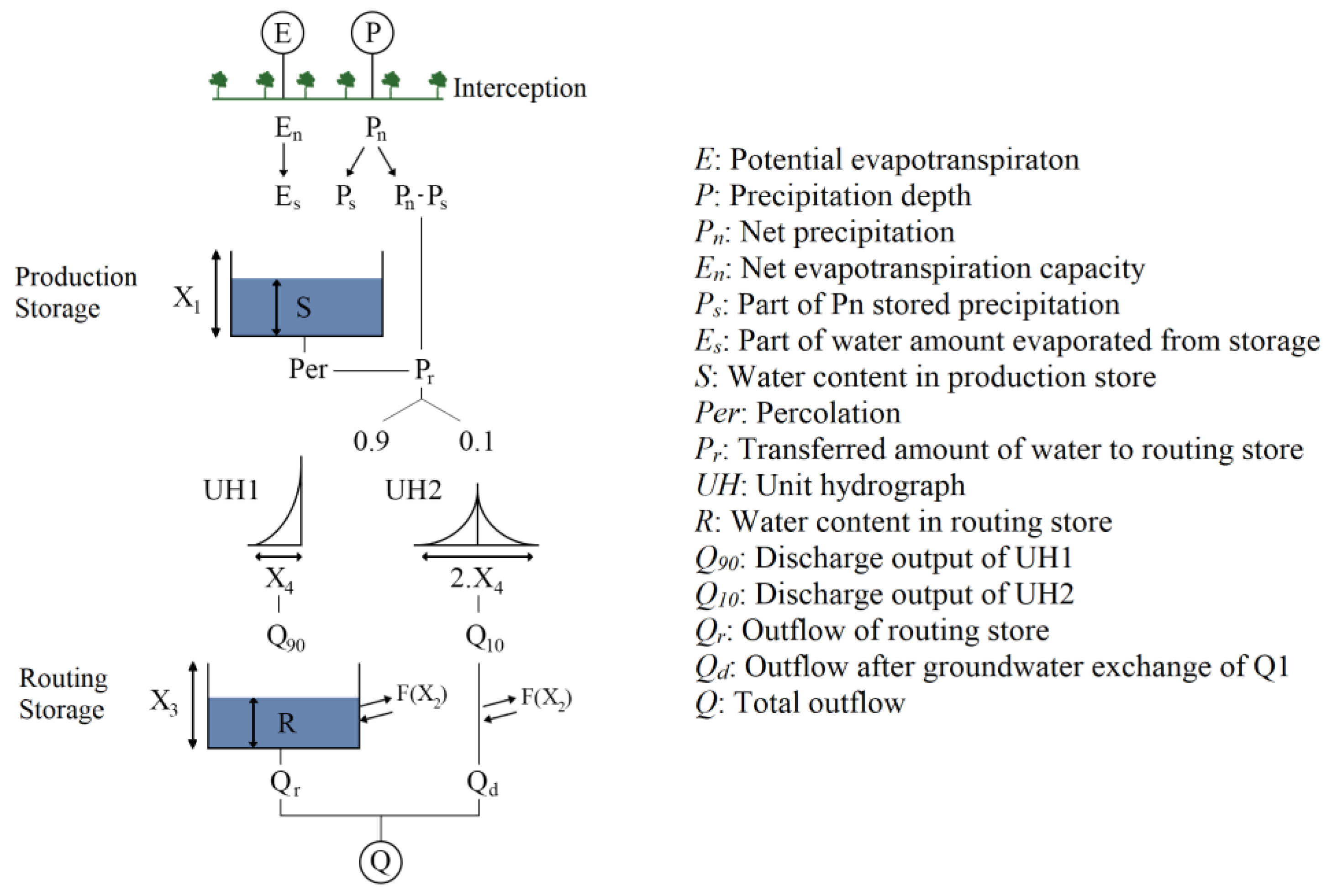
GR4J conducts the process that represents the rainfall–runoff relationship via 2 box model methods, which are called production storage and routing storage. The structure of the model is given in Figure 4. As the precipitation reaches the surface, the first unit of the model that meets the water mass after the interception process is production storage. The largest amount of net precipitation after infiltration is transferred to routing storage by using the unit hydrograph method. Then, the remaining net precipitation is routed by a unit hydrograph the base width of which is twice that of the previous step. Finally, the amount of water coming from routing storage and the routed part of the remaining net precipitation merge. The summation of these values ends up with the output of GR4J, which is discharge.

2.3.2. SWAT+

A soil water assessment tool was developed by Dr. Jeff Arnold as a result of his research conducted for the USDA-ARS (U.S. Department of Agriculture—Agricultural Research Service) to foresee the effects of land use and management in a basin with a heterogeneous structure [17]. In addition to being a physically based model, SWAT is a semi-distributed and continuous hydrological model working at a daily time-step which has a wide use area such as rainfall–runoff relationship, climate change, and environmental studies at small or large basins [18,19,20]. The semi-distributed structure of the model consists of sub-basins and hydrologic response units (HRUs) in detail. In earlier versions of the SWAT model, the smallest spatial sub-division of a basin is represented by HRUs. As a new feature in SWAT+, HRUs are divided into landscape units (LSUs). LSUs are divided into two parts, namely, upland and floodplain. The HRUs are homogenous in themselves in terms of their physical characteristics [21]. We used QGIS software and QSWAT+ plugin in this study to set up the model because of its easy-to-use interface and its being the most up-to-date version of the SWAT+ model. It requires DEM, land use, and a soil map as physical data, and precipitation, temperature, wind speed, solar radiation, and relative humidity as climatic and hydrological data. Although SWAT+ can automatically calculate PET with different methods, we added the ERA5 PET data to compare results fairly with other models. We only focused on the discharge output of the SWAT+ model in line with our objective. The discharge value was obtained at the outlet location by routing the output of each HRU individually through the main outlet. During the modelling process, we divided the Acısu Basin into 5 sub-basins and 1981 HRUs ranging in surface area from 6 to 60.26 km². SWAT+ conducts the process in two phases, namely, the land phase and routing phase. Considering the information given in [22], we used the SCS-CN (Soil Conservation Service—Curve Number) method in the land phase, and the Muskingum method in the routing phase.

2.3.3. mHM

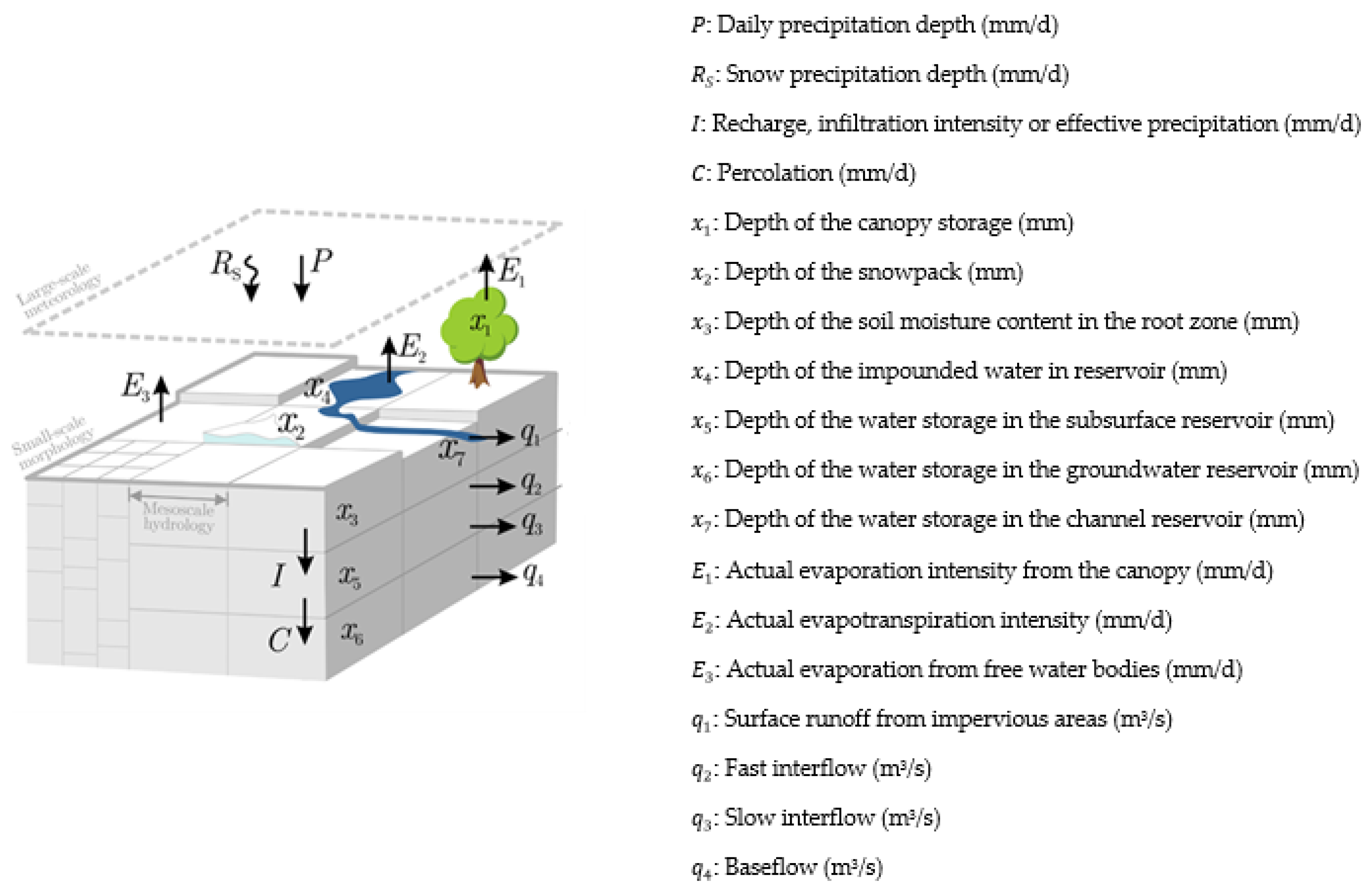
The mesoscale Hydrologic Model (mHM) is a distributed, physically based and continuous hydrologic model published by a team from UFZ (Helmholtz Centre for Environmental Research) [23,24]. The fundamental numerical approaches regarding the hydrologic processes of the mHM are tested by using well-known and acknowledged lumped models such as HBV [25] and VIC [26]. The input and parameter variety for each grid of mHM set this model apart from other rainfall–runoff models. With this difference, changes in characteristics of the basin can be better represented as the spatial resolution of the model run and forcing data increases. We ran the model at 0.015625 degrees (~2 km) spatial resolution, which is assumed to be appropriate for the study area. We used ERA5 meteorological forcings at 0.25 degrees. We also used high resolution soil data at 0.001953125 degrees (~200 m). We used the multi-parameter regionalization (MPR) approach [27] and a new routing scheme, i.e., adaptive timestep, spatially varying celerity [28]. The model structure is given in Figure 5.

All processes are applied in each cell individually, and the continuity of the model is provided by using ordinary differential equations (ODE). The results of ODEs obtained from each cell are routed by using the Muskingum method through the main outlet [29].

In this study, open-source Fortran based code of mHM is compiled with Cygwin to run the model in Windows environment.

2.4. Calibration of Models

2.4.1. Sensitivity Analysis

Sensitivity analyses and calibrations of the examined models are performed by using the Parameter Estimation Tool (PEST), which is a model-independent auto-calibration tool [30]. Sensitivity analysis is used to indicate the effect of a change in parameter value to objective function. The main purpose of using this method is to eliminate ineffective parameters before the calibration process to avoid wasting time on unnecessary iterations. In this study, sensitivity analysis of the models’ parameters is performed using the auto-sensitivity module of PEST. It is basically based on the equation given below:

$$S=\frac{\mathsf{\Delta } OF (\%)}{\mathsf{\Delta } Par (\%)}$$

(1)

where S is sensitivity value, “ΔOF” is change in objective function as percentage corresponding to parameter change, and “ΔPar” is change in parameter value as percentage.

2.4.2. Calibration Algorithms

Calibration is a process which is performed to obtain optimum results from models by adjusting parameter values. The calibration of each model’s parameters was performed by using three algorithms of PEST, namely, Levenberg–Marquardt (LM), Shuffled Complex Evolution (SCE), and Covariance Matrix Adoption Evolution Strategy (CMAES). These are classified as local and global algorithms. LM is a local optimization algorithm which is composed of gradient descent and Gauss–Newton methods [31]. SCE and CMAES are global optimization algorithms. SCE is a combination of the competitive evolution, the local direct search of downhill simplex method, a controlled random search, and the concept of complex shuffling [32]. Finally, CMAES is another global optimization algorithm including stochastic approaches and non-linear functions. It uses the maximum likelihood method to attain parameter values, thereby giving results closer to the optimum solution in previous iterations [33].

3. Results

3.1. Sensitivity Analysis

To define the effectiveness of the parameters on the models’ objective, sensitivity analysis was performed for GR4J, SWAT+, and mHM. Four parameters of GR4J, 20 parameters of SWAT+ affecting discharge [34], and 66 parameters of mHM were involved in this process to eliminate unsensitive components. The sensitivity analysis of this study was completed by using auto-sensitivity analysis of PEST for the calibration period (1991–2000). The threshold of the sensitivity value was selected as 0.0025 subjectively using the information shared in [35]. The results of the sensitivity analysis are given in Figure 6, Figure 7 and Figure 8.

For the Acısu Basin, the results of the sensitivity analysis showed that the most effective parameter is “X2” which is the change in groundwater storage for GR4J, and three out of four parameters of the GR4J model were defined as sensitive.

The SWAT+ sensitivity analysis results demonstrated that “cn2” (SCS curve number) is the most sensitive parameter in discharge. The sensitivity analysis of SWAT+ was performed using 20 parameters, and 11 out of 20 parameters above the threshold were selected as sensitive. Descriptions of the sensitive parameters were given in

Table 3. SWAT+ parameter descriptions.

Parameter	Desscription	Unit
cn2	SCS curve number	-
awc	Soil water content	-
k	Hydraulic conductivity of saturated soil	mm/hr
perco	Percolation coefficient	-
revap	Evaporation coefficient from shallow aquifer to root	-
canmx	Maximum canopy storage	mm
esco	Soil evaporation compensation factor	-
epco	Plant uptake compensation factor	-
evrch	Reach evaporation adjustment factor	-
flomin	Minimum amount of water to be stored in the aquifer for return flow	mm
revap_min	Minimum water depth required in shallow aquifer for “revap”	mm

for SWAT+.

Finally, mHM sensitivity analysis resulted in 15 sensitive parameters out of 69 parameters. The most sensitive parameter of mHM is “PTF_lower66_5_clay” which is a coefficient of the pedotransfer function for soil including clay lower than 66.5%. Descriptions of sensitive parameters are given in

Table 4. mHM parameter descriptions.

Parameter	Parameter Description
PTF_lower66_5_clay	Pedotransfer function (PTF) soil moisture constant for less than 66.5% clay
PTF_Ks_sand	PTF hydraulic conductivity constant for saturated sand
PTF_Ks_clay	PTF hydraulic conductivity constant for saturated clay
rootFractionCoefficient_pervious	Root fraction coefficient for pervious area
PTF_lower66_5_Db	PTF density constant for less than 66.5% sand
PTF_lower66_5_constant	PTF soil moisture constant for less than 66.5% sand
PTF_Ks_constant	PTF hydraulic conductivity constant for saturated soil
rootFractionCoefficient_forest	Root fraction coefficient for forest
infiltrationShapeFactor	Shape factor that divides effective precipitation into infiltration and surface flow
PET_a_forest	Forest—PET correction factor
PET_a_pervious	Pervious area—PET correction factor
PET_b	Agricultural land—PET correction factor
PET_c	Agricultural land—PET correction factor (2)
canopyInterceptionFactor	Canopy interception factor
exponentSlowInterflow	Slow interflow exponent

for mHM. These results show that soil-related parameters at each model are dominant for the study area.

3.2. Calibration and Validation

The sensitive parameters were used in the calibration period from 1991 to 2000 and the validation period from 2002 to 2005 with daily time-step for each model. GR4J, SWAT+, and mHM were integrated with PEST to calibrate and validate these models by using three optimization algorithms—namely, Levenberg–Marquardt (LM), shuffled complex evolution (SCE), and covariance matrix adoption evolution strategy (CMAES). These algorithms have some common limitations. The limitations were defined similarly for each algorithm for fair comparison. The maximum iteration number was defined as 1000 and termination criteria were defined as lower than 10–6 change in the objective function (NSE) through 15 successive iterations for all three algorithms.

To assess discharge simulation performance, the calibration process was accomplished on a daily time basis for the models. The resultant parameter values and defined parameter boundaries are given in

Table 5. Calibrated parameters of each model.

Model	Parameter	Calibrated Value			Limit
		L-M	SCE-UA	CMAES	Min	Max
GR4J	X1	399.99	346.37	347.02	10	2000
	X2	0.00	0.46	0.47	−8	6
	X3	10.00	10.00	10.00	10	500
	X4	1.77	1.32	1.33	1	4
SWAT+	cn2	0.77	0.67	0.68	0.65	0.95
	awc	0.02	0.01	0.01	0.01	0.51
	k	200.40	189.18	193.07	0.00	2000.00
	perco	0.28	0.16	0.20	0.00	1.00
	revap	0.20	0.05	0.16	0.02	0.20
	canmx	19.99	23.55	22.33	0.00	100.00
	esco	0.67	0.37	0.39	0.00	1.00
	epco	0.04	0.17	0.17	0.00	1.00
	evrch	0.67	0.75	0.56	0.50	1.00
	flomin	500.00	355.52	1059.35	0.00	1250.00
mHM	PTF_lower66_5_clay	0.0017	0.0012	0.0019	0.0001	0.0029
	PTF_Ks_sand	0.0083	0.0221	0.0158	0.0060	0.0260
	PTF_Ks_clay	0.0079	0.0130	0.0124	0.0030	0.0130
	rootFractionCoefficient_pervious	0.0608	0.0095	0.0460	0.0010	0.0900
	PTF_lower66_5_Db	−0.3463	−0.2141	−0.2315	−0.5513	−0.0913
	PTF_lower66_5_constant	0.6877	0.6724	0.6750	0.5358	1.1232
	PTF_Ks_constant	−0.7105	−1.1978	−1.0251	−1.2000	−0.2850
	rootFractionCoefficient_forest	0.9401	0.9623	0.9872	0.9000	0.9990
	infiltrationShapeFactor	1.9602	1.1113	1.0000	1.0000	4.0000
	PET_a_forest	0.7221	1.2466	1.2885	0.3000	1.3000
	PET_a_pervious	0.7414	0.3604	0.3176	0.3000	1.3000
	PET_b	0.6823	0.7020	0.5982	0.0000	1.5000
	PET_c	−0.9670	−0.0001	−0.0427	−2.0000	0.0000
	canopyInterceptionFactor	0.1520	0.1501	0.2135	0.1500	0.4000
	exponentSlowInterflow	0.1948	0.2324	0.2054	0.0500	0.3000

for GR4J, SWAT+, and mHM.

Using the parameter values shown in the tables above, GR4J, SWAT+, and mHM were run for calibration and validation periods. According to the NSE values which were calculated for discharge outputs that belong to each model–algorithm combination,

Table 6. Calibration results.

Calibratoin 1991–2000	NSE	R2	KGE	RSR	PBIAS	MSE	RMSE
mHM-CMAES	0.67	0.66	0.74	0.58	2.0	77.84	8.82
mHM-SCE	0.67	0.67	0.74	0.57	−1.9	76.59	8.75
GR4J-SCE	0.63	0.63	0.72	0.61	0.4	86.29	9.29
GR4J-CMAES	0.63	0.63	0.72	0.61	0.4	86.29	9.29
SWAT+-SCE	0.56	0.57	0.72	0.66	−2.0	102.76	10.14
SWAT+-CMAES	0.56	0.57	0.72	0.67	2.8	103.13	10.16
mHM-LM	0.54	0.55	0.71	0.68	−1.5	108.23	10.40
SWAT+-LM	0.53	0.55	0.70	0.68	−3.4	108.32	10.41
GR4J-LM	0.44	0.59	0.22	0.75	−55.5	131.05	11.45

and

Table 7. Validation results.

Validation 2002–2005	NSE	R2	KGE	RSR	PBIAS	MSE	RMSE
mHM-CMAES	0.60	0.61	0.61	0.63	−9.9	52.96	7.28
mHM-SCE	0.56	0.58	0.55	0.67	−16.6	58.63	7.66
GR4J-LM	0.55	0.62	0.44	0.67	−42.7	59.24	7.70
GR4J-SCE	0.44	0.67	0.60	0.75	23.5	73.77	8.59
GR4J-CMAES	0.44	0.67	0.60	0.75	23.5	73.50	8.57
SWAT+-SCE	0.38	0.41	0.57	0.79	−2.4	81.58	9.03
SWAT+-CMAES	0.38	0.41	0.60	0.78	0.2	81.36	9.02
SWAT+-LM	0.35	0.40	0.54	0.81	−9.4	86.29	9.29
mHM-LM	0.31	0.37	0.53	0.83	−20.4	91.59	9.57

were arranged and given with other statistical performance indicators.

As shown in Table 6 and Table 7, model–algorithm combinations were ordered by their NSE values. Calibrating using, respectively, LM, SCE, and CMAES, GR4J has an NSE value of 0.44, 0.63, and 0.63; SWAT+ has 0.53, 0.56, and 0.56; mHM has 0.54, 0.67, and 0.67.

For the validation period with, respectively, LM, SCE, and CMAES, GR4J has NSE value of 0.55, 0.44, and 0.44; SWAT+ has 0.35, 0.38, and 0.38; mHM has 0.31, 0.56, and 0.60. Iterations are continuously completed for all of the combinations with PEST. From the aspect of performance evaluation, mHM-CMAES integration has shown “good” performance according to the classification given in

Table 8. Classification of discharge simulation performance.

Performance	RSR	NSE	PBIAS
Very Good	0.00 ≤ RSR ≤ 0.50	0.70 < NSE ≤ 1.00	PBIAS < ±10
Good	0.50 < RSR ≤ 0.60	0.65 < NSE ≤ 0.75	±10 ≤ PBIAS < ±15
Satisfactory	0.60 < RSR ≤ 0.70	0.50 < NSE ≤ 0.65	±15 ≤ PBIAS < ±25
Poor	RSR > 0.70	NSE ≤ 0.5	PBIAS ≥ ±25

and presented in [36].

A comparison of these statistical findings was supported with a bar chart in Figure 9 and Figure 10 to virtualize model and algorithm performances with their average NSE values for calibration and validation processes, respectively.

What stands out in Figure 9 is that SCE’s and CMAES’s NSE values are close to each other. SCE and CMAES have average NSE values as 0.62 and outperformed LM, which has a 0.50 average NSE value after calibration.

CMAES dominated other algorithms in validation with an average NSE value of 0.47, whilst SCE has 0.46 and LM has 0.40 average NSE values as can be seen in Figure 10. In model basis, mHM outperformed other two models with an average NSE value of 0.63. SWAT+ and GR4J have average NSE values of 0.37 and 0.48, respectively. By the end of the comparison process, the hydrograph of the best combination is given in Figure 11.

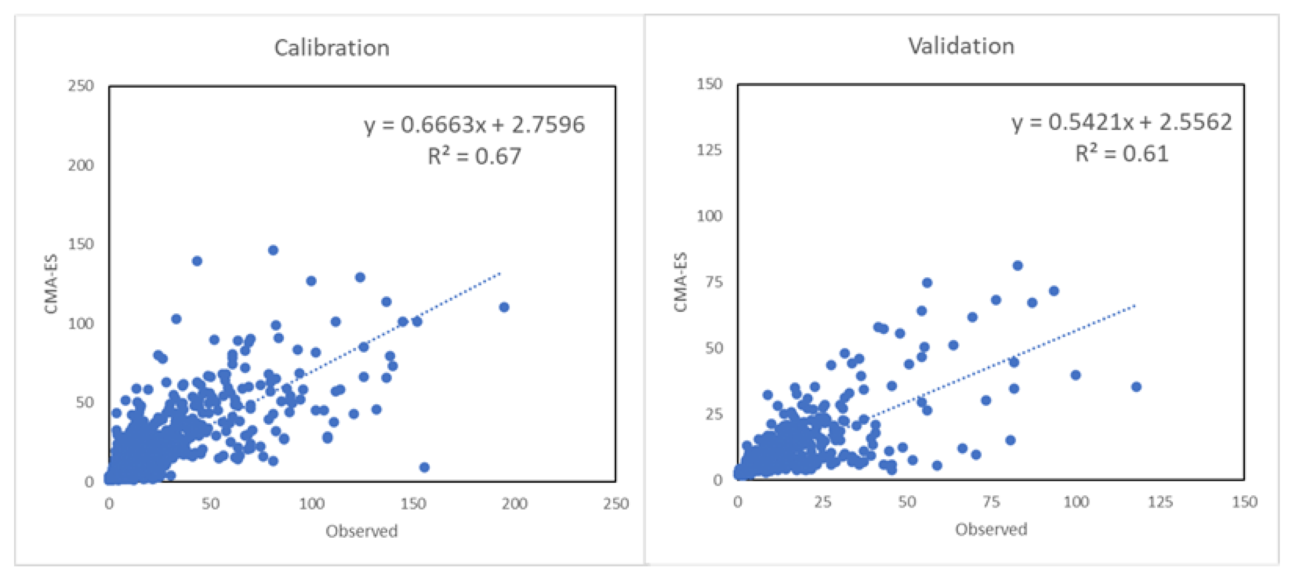
As shown in Figure 11, the resultant hydrograph with the highest NSE value in general is the mHM–CMAES combination. Besides reaching 0.67 and 0.60 NSE values, respectively, it has 0.67 and 0.61 R² values, which is shown Figure 12 with scatter plots.

In line with hydrographs, the distribution of calibrated and validated values demonstrates that simulated values are mostly lower than observed values.

Additionally, SWAT+ and mHM can present visual results for various outputs—i.e., discharge, potential evapotranspiration, snowpack, and soil moisture content. In Figure 13, the annual output of each model for the last year of validation (2005) is given as maps to visualize the discharge distribution in the study domain. A representative map of GR4J output is given for comparing the distributed structure of the models.

4. Discussion

Hydrological model selection is a key factor for decision makers in the planning and management of water resources. Hydrological models have various strengths and limitations depending on their model structure, model inputs, and their ability to represent the nature of the hydrological phenomenon. Basically, they convert rainfall to runoff, route in the channels, and are mainly used for predictions and forecasts using forecasted weather inputs. All performed model–algorithm integrations captured the discharge pattern for the Acısu Basin except for the first year of validation (Figure 11). This inaccuracy may be related to the excluded period of 2001–2002. This exclusion was made to significantly avoid the negative impact of this period on the calibration process. Moreover, Table 1 shows that the ERA5 dataset has almost 20% less annual precipitation and higher temperatures leading to more potential evapotranspiration. In line with these details, the models produced less discharge than expected.

In general, the model and three different calibration algorithm capabilities were tested for the study area. The findings showed that the results of the combinations are close to the results of the studies performed for the Acısu Basin and surrounding area [15,37] for similar methods. The main differences between the model structures in this study are their spatial resolutions and model complexity. GR4J is a lumped model, whereas SWAT+ is a semi-distributed model. Since mHM is a distributed hydrological model, the model structure is more sensitive to the input data and its resolution for representing the characteristics of the basin. Most importantly, users can retrieve flux and state simulations from any location in the basin. On the other hand, GR4J and SWAT+ have limitations in defining meteorological inputs as spatially distributed. These models can involve meteorological inputs in the process as time series. GR4J allows users to define single time series for the whole basin, while SWAT+ gives the opportunity to add inputs at different locations.

One of the general results presented in the literature is that the error values decrease by using the average of the spatial values of the basin in the lumped models compared to the distributed models. As a result of the analyses in this study, contrary to the aforementioned situation, the distributed model (mHM) shows better discharge simulation performance than the lumped and semi-distributed models according to NSE. When the obtained data and results were examined, it was concluded that this was due to the heterogeneous structure of the basin and that the model structure of mHM more successfully defines the basin characteristics in terms of the resolution which it processes heterogeneity. Although the reanalysis data of the ERA5 or coarse soil map may be insufficient as resolution or for this specific study area due to its small surface area, mHM still simulated the discharge better than the other two models. The reason for this result may be the model’s skillful multi-parameter regionalization algorithm (MPR) capturing the heterogeneity of the basin characteristics with a limited number of calibrated parameters. This approach is a unique feature of mHM as compared to the other distributed models.

The modelling procedure needs fine-tuning of the model parameters to come closer to the optimum. This process is known as calibration. Both local (LM) and global (SCE, CMAES) algorithms were applied to the hydrological models in this study. Results are given in Table 6 and Table 7. Global algorithms provide a comprehensive search for the optimum parameter set. As it is expected considering previous studies [14,32], SCE and CMAES ended with better results than LM while CMAES was the best.

The Acısu Basin has an important location at the upstream of the Gediz Basin, which is one of the largest basins in Turkey. Hydrological model studies in this region have priority for irrigation because of its agricultural potential [38,39,40]. For this reason, it is thought that alternative modeling approaches will guide researchers for studies to be carried out in the basin. Therefore, modelling studies can be directive for researchers for the basin. We aimed to facilitate the method selection for decision makers.

5. Conclusions

As a developing country, the population and thus the need for industrial, irrigation and drinking water is increasing rapidly in Turkey. For this reason, the importance of studies on water resources for the effective use of water is increasing day by day. The Gediz Basin is especially important in hydrological studies due to its agricultural land and potential drought risk. To assess future conditions, hydrological models are preliminary tools. For the purpose of facilitating the selection of a hydrological model and its calibration algorithm, three hydrological model structures (lumped, semi distributed, distributed) and three algorithms (LM, SCE, CMAES) were compared with nine combinations in this study. Based on the comparison and results, the following conclusions can be drawn:

• In contrast to general findings, the distributed model (mHM) simulated the discharge with higher performance than the coarser models (SWAT+ and GR4J).
• Global optimization algorithms (CMAES and SCE) have extensive ability to search for the optimum parameter set compared to a local algorithm (LM). The highest performance was shown by CMAES based on average NSE through calibration and validation.
• In terms of time efficiency, each model has a different run-time for the study domain. A single run takes an average of 30 s for mHM, 2 min for SWAT+, and 4 s for GR4J.
• Since mHM and SWAT+ allows the drawing of outputs for any sub-basin located at the upstream, it is advantageous compared to GR4J under data-limited modelling conditions.
• The resultant hydrographs demonstrated that simulated discharge values were lower than observed values in general. The reason for this is related to the difference between ERA5 data and MGM measurements. The direct relationship between precipitation and discharge leads the models to simulate lower values.

The results obtained with the applied models and algorithms are limited to the Acısu Basin. In order to generalize the results, it is recommended that the basins with different geographical, meteorological, and geological characteristics with similar models and algorithms be examined. The modelers should identify the priorities of the modeling practice and select the right model for the right purpose. Input demands can be covered by open-source global data sources and currently the distributed model can easily be set up for any location in the world. However, if only flood forecasting is the aim and process understanding is not necessary, relatively simple models can be utilized for a quick solution for the domain. Future work should focus on appropriate model structure selection for flood or drought forecasting using ERA5 land inputs and ECMWF forecasted meteorological forcing.

References

- Pechlivanidis, I.G.; Jackson, B.M.; Mcintyre, N.R.; Wheater, H.S. Catchment scale hydrological modelling: A review of model types, calibration approaches and uncertainty analysis methods in the context of recent developments in technology and applications. Glob. Nest J. 2011, 13, 193–214. [Google Scholar] [CrossRef]
- Foughali, A.; Tramblay, Y.; Bargaoui, Z.; Carreau, J.; Ruelland, D. Hydrological Modeling in Northern Tunisia with Regional Climate Model Outputs: Performance Evaluation and Bias-Correction in Present Climate Conditions. Climate 2015, 3, 459–473. [Google Scholar] [CrossRef] [Green Version]
- Mulvaney, T.J. On the use of self registering rain and flood gauges in making observations of the relation of rainfall and flood discharges in given catchment. Trans. Instit. Civ. Eng. Irel. 1850, 4, 18–33. [Google Scholar]
- Crawford, N.H.; Linsley, R.K. Digital Simulation in Hydrology’Stanford Watershed Model 4; Stanford University: Stanford, CA, USA, 1966. [Google Scholar]
- De Luca, D.L.; Apollonio, C.; Petroselli, A. The Benefit of Continuous Hydrological Modelling for Drought Hazard Assessment in Small and Coastal Ungauged Basins: A Case Study in Southern Italy. Climate 2022, 10, 34. [Google Scholar] [CrossRef]
- Tegegne, G.; Park, D.K.; Kim, Y.O. Comparison of hydrological models for the assessment of water resources in a data-scarce region, the Upper Blue Nile River Basin. J. Hydrol. Reg. Stud. 2017, 14, 49–66. [Google Scholar] [CrossRef]
- Brulebois, E.; Ubertosi, M.; Castel, T.; Richard, Y.; Sauvage, S.; Sanchez-Perez, J.-M.; Moine, N.L.; Amiotte-Suchet, P. Robustness and performance of semi-distributed (SWAT) and global (GR4J) hydrological models throughout an observed climatic shift over contrasted French watersheds. Open Water J. 2018, 5, 41–56. [Google Scholar]
- Kunnath-Poovakka, A.; Eldho, T.I. A comparative study of conceptual rainfall-runoff models GR4J, AWBM and Sacramento at catchments in the upper Godavari river basin, India. J. Earth Syst. Sci. 2019, 128, 33. [Google Scholar] [CrossRef] [Green Version]
- Mai, J.; Tolson, B.A.; Shen, H.; Gaborit, É.; Fortin, V.; Gasset, N.; Awoye, H.; Stadnyk, T.A.; Fry, L.M.; Bradley, E.A.; et al. Great Lakes Runoff Intercomparison Project Phase 3: Lake Erie (GRIP-E). J. Hydrol. Eng. 2021, 26, 05021020. [Google Scholar] [CrossRef]
- Duan, Q.; Gupta, H.V.; Sorooshian, S.; Rousseau, A.N.; Turcotte, R. Calibration of Watershed Models; John Wiley & Sons: Hoboken, NJ, USA, 2003; Volume 6. [Google Scholar]
- Azar, A.T.; Khan, Z.I.; Amin, S.U.; Fouad, K.M. Hybrid Global Optimization Algorithm for Feature Selection. Comput. Mater. Contin. 2023, 74, 2021–2037. [Google Scholar] [CrossRef]
- Wallner, M.; Haberlandt, U.; Dietrich, J. Evaluation of different calibration strategies for large scale continuous hydrological modelling. Adv. Geosci. 2012, 31, 67–74. [Google Scholar] [CrossRef] [Green Version]
- Demirel, M.C.; Özen, A.; Orta, S.; Toker, E.; Demir, H.K.; Ekmekcioğlu, Ö.; Tayşi, H.; Eruçar, S.; Sağ, A.B.; Sarı, Ö.; et al. Additional Value of Using Satellite-Based Soil Moisture and Two Sources of Groundwater Data for Hydrological Model Calibration. Water 2019, 11, 2083. [Google Scholar] [CrossRef] [Green Version]
- Yılmaz, M.; Alp, H.; Tosunoğlu, F.; Aşıkoğlu, Ö.L.; Eriş, E. Impact of climate change on meteorological and hydrological droughts for Upper Coruh Basin, Turkey. Nat. Hazards 2022, 112, 1039–1063. [Google Scholar] [CrossRef]
- Kumanlioglu, A.A.; Fistikoglu, O. Performance Enhancement of a Conceptual Hydrological Model by Integrating Artificial Intelligence. J. Hydrol. Eng. 2019, 24, 04019047. [Google Scholar] [CrossRef]
- Perrin, C.; Michel, C.; Andréassian, V. Improvement of a parsimonious model for streamflow simulation. J. Hydrol. 2003, 279, 275–289. [Google Scholar] [CrossRef]
- Arnold, J.G.; Srinivasan, R.; Muttiah, R.S.; Williams, J.R. Large Area Hydrologic Modeling and Assessment Part I: Model DevelopmenT. J. Am. Water Resour. Assoc. 1998, 34, 73–89. [Google Scholar] [CrossRef]
- Gebrechorkos, S.H.; Bernhofer, C.; Hülsmann, S. Climate change impact assessment on the hydrology of a large river basin in Ethiopia using a local-scale climate modelling approach. Sci. Total Environ. 2020, 742, 140504. [Google Scholar] [CrossRef]
- Peker, I.B.; Sorman, A.A. Application of SWAT using snow data and detecting climate change impacts in the mountainous eastern regions of Turkey. Water 2021, 13, 1982. [Google Scholar] [CrossRef]
- Anjum, M.N.; Ding, Y.; Shangguan, D. Simulation of the projected climate change impacts on the river flow regimes under CMIP5 RCP scenarios in the westerlies dominated belt, northern Pakistan. Atmos. Res. 2019, 227, 233–248. [Google Scholar] [CrossRef]
- Dile, Y.T.; Daggupati, P.; George, C.; Srinivasan, R.; Arnold, J. Introducing a New Open Source GIS User Interface for the SWAT Model. Environ. Model. Softw. 2016, 85, 129–138. [Google Scholar] [CrossRef]
- Rostamian, R.; Jaleh, A.; Afyuni, M.; Mousavi, S.F.; Heidarpour, M.; Jalalian, A.; Abbaspour, K.C. Application of a SWAT Model for Estimating Runoff and Sediment in Two Mountainous Basins in Central Iran. Hydrol. Sci. J. 2008, 53, 977–988. [Google Scholar] [CrossRef]
- Samaniego, L.; Kumar, R.; Attinger, S. Multiscale parameter regionalization of a grid-based hydrologic model at the mesoscale. Water Resour. Res. 2010, 46, W05523. [Google Scholar] [CrossRef] [Green Version]
- Kumar, R.; Samaniego, L.; Attinger, S. Implications of distributed hydrologic model parameterization on water fluxes at multiple scales and locations. Water Resour. Res. 2013, 49, 360–379. [Google Scholar] [CrossRef]
- Bergström, S. The HBV model—Its structure and applications. Swed. Meteorol. Hydrol. Inst. Norrköping 1992, 4, 1–33. [Google Scholar]
- Liang, X.; Wood, E.F.; Lettenmaier, D.P. Surface soil moisture parameterization of the VIC-2L model: Evaluation and modification. Glob. Planet. Change 1996, 13, 195–206. [Google Scholar] [CrossRef]
- Schweppe, R.; Thober, S.; Müller, S.; Kelbling, M.; Kumar, R.; Attinger, S.; Samaniego, L. MPR 1.0: A stand-alone multiscale parameter regionalization tool for improved parameter estimation of land surface models. Geosci. Model Dev. 2022, 15, 859–882. [Google Scholar] [CrossRef]
- Thober, S.; Cuntz, M.; Kelbling, M.; Kumar, R.; Mai, J.; Samaniego, L. The multiscale routing model mRM v1.0: Simple river routing at resolutions from 1 to 50 km. Geosci. Model Dev. 2019, 12, 2501–2521. [Google Scholar] [CrossRef] [Green Version]
- Demirel, M.C.; Mai, J.; Mendiguren, G.; Koch, J.; Samaniego, L.; Stisen, S. Combining satellite data and appropriate objective functions for improved spatial pattern performance of a distributed hydrologic model. Hydrol. Earth Syst. Sci. 2018, 22, 1299–1315. [Google Scholar] [CrossRef] [Green Version]
- Doherty, J.; Johnston, J.M. Methodologies for calibration and predictive analysis of a watershed model. J. Am. Water Resour. Assoc. 2003, 39, 251–265. [Google Scholar] [CrossRef]
- Mehrdoust, F.; Noorani, I.; Hamdi, A. Two-Factor Heston Model Equipped with Regime-Switching: American Option Pricing and Model Calibration by Levenberg–Marquardt Optimization Algorithm. Math. Comput. Simul. 2023, 204, 660–678. [Google Scholar] [CrossRef]
- Shoarinezhad, V.; Wieprecht, S.; Haun, S. Comparison of local and global optimization methods for calibration of a 3D morphodynamic model of a curved channel. Water 2020, 12, 1333. [Google Scholar] [CrossRef]
- Patel, S.; Eldho, T.I.; Rastogi, A.K.; Rabinovich, A. Groundwater Parameter Estimation Using Multiquadric-Based Meshfree Simulation with Covariance Matrix Adaptation Evolution Strategy Optimization for a Regional Aquifer System. Hydrogeol. J. 2022, 30, 2205–2221. [Google Scholar] [CrossRef]
- Arnold, J.G.; Moriasi, D.N.; Gassman, P.W.; Abbaspour, K.C.; White, M.J.; Srinivasan, R.; Santhi, C.; Harmel, R.D.; van Griensven, A.; Van Liew, M.W.; et al. Swat: Model Use, Calibration, and Validation. Trans. ASABE 2012, 55, 1491–1508. [Google Scholar] [CrossRef]
- Feyereisen, G.W.; Strickland, T.C.; Bosch, D.D.; Sullivan, D.G. Evaluation of SWAT Manual Calibration and Input Parameter Sensitivity in the Little River Watershed. Trans. ASABE 2007, 50, 843–855. [Google Scholar] [CrossRef]
- Moriasi, D.N.; Gitau, M.W.; Pai, N.; Daggupati, P. Hydrologic and water quality models: Performance measures and evaluation criteria. Trans. ASABE 2015, 58, 1763–1785. [Google Scholar] [CrossRef] [Green Version]
- Okkan, U.; Ersoy, Z.B.; Ali Kumanlioglu, A.; Fistikoglu, O. Embedding machine learning techniques into a conceptual model to improve monthly runoff simulation: A nested hybrid rainfall-runoff modeling. J. Hydrol. 2021, 598, 126433. [Google Scholar] [CrossRef]
- Kilic, M.; Tuylu, G.I. Determination of water conveyance loss in the ahmetli regulator irrigation system in the lower Gediz Basin Turkey. Irrig. Drain. 2011, 60, 579–589. [Google Scholar] [CrossRef]
- Karatas, B.S.; Akkuzu, E.; Unal, H.B.; Asik, S.; Avci, M. Using satellite remote sensing to assess irrigation performance in Water User Associations in the Lower Gediz Basin, Turkey. Agric. Water Manag. 2009, 96, 982–990. [Google Scholar] [CrossRef]
- Tonkul, S.; Baba, A.; Şimşek, C.; Demirkesen, A.C. Groundwater recharge estımatıon ın the Alaşehir sub-basın usıng hydro-geochemical data; Alaşehir case study. Environ. Earth Sci. 2021, 80, 261. [Google Scholar] [CrossRef]
Figure 1.
Study domain.
Figure 2.
Comparison of MGM and ERA5 data.
Figure 3.
Observed discharge data of gauge 523.
Figure 4.
GR4J model structure.
Figure 5.
mHM cell structure.
Figure 6.
GR4J sensitivity analysis results.
Figure 7.
SWAT+ sensitivity analysis results.
Figure 8.
mHM sensitivity analysis results.
Figure 9.
Calibration performance for each algorithm.
Figure 10.
Validation performances for each algorithm.
Figure 11.
Comparison of observed discharge data with mHM–CMAES simulation results.
Figure 12.
Scatter diagram of observed and simulated discharge data.
Figure 13.
Map outputs of each model.