Article

The Relevance of the Low-Frequency Sound Insulation of Window Elements of Façades on the Perception of Urban-Type Sounds

by
Daniel de la Prida
1,2,*,†,
María Ángeles Navacerrada
1,*,†,
María Aguado-Yáñez
1,
Luis Antonio Azpicueta-Ruiz
2,
Antonio Pedrero
1 and
David Caballol
1
1
Grupo de Investigación en Acústica Arquitectónica, Universidad Politécnica de Madrid, CP: 28040 Madrid, Spain
2
Signal Theory and Communications Department, Universidad Carlos III de Madrid, CP: 28911 Madrid, Spain
*
Authors to whom correspondence should be addressed.
These authors contributed equally to this work.
Buildings 2023, 13(10), 2561; https://doi.org/10.3390/buildings13102561
Submission received: 3 August 2023 / Revised: 4 October 2023 / Accepted: 7 October 2023 / Published: 10 October 2023
(This article belongs to the Special Issue Acoustics and Noise Control in Buildings)

Abstract

:
The sound insulation of the façade and its elements is a very important characteristic, as it largely determines the degree of sound protection of the building’s interior from external noise sources. This feature, therefore, has a great influence on the acoustic comfort and health of the occupants. For this reason, it is very important that the way in which the sound insulation of the façade is quantified and represented corresponds to the way it is perceived. Although there have long been regulations describing how it should be measured and expressed through Single-Number Quantities (SNQs), there is much scientific debate about the appropriateness of current standardised methods for expressing sound insulation, in terms of whether they accurately represent human-perceived comfort. In this regard, much of the debate centres on the frequency range to be considered when expressing sound insulation, with no consensus as to whether the low-frequency bands (i.e., 50, 63, and 80 Hz) should be used for the calculation of façade sound insulation SNQs. In order to contribute to this knowledge, we conducted a listening test using a Two-Alternative Choice (2-AC) protocol on a sample of 100 participants to test whether participants’ annoyance with urban noise changed significantly with variations in window sound insulation only in the low-frequency range. The results of the experiment, analysed using Thurstonian models, showed that the influence of low frequencies is limited for the sound insulation of the tested window façade elements and urban-type noise of aircraft and mixed urban traffic at low speeds and only becomes relevant when the sound insulation of the elements is exceptionally low in the low-frequency range.

1. Introduction

The sound insulation of building construction elements has a direct impact on the spectral sound levels transmitted from the outside into a given enclosure separated from other enclosures or from the outside by walls or other types of structural partitions.
Being such an important characteristic, regulations have been developed over the years to describe how to measure it accurately [1,2,3]. In addition, SNQ calculation standards have been developed [4], to describe the sound insulation of elements by a single number, taking into account the spectral behaviour of the sound insulation and which can be adapted to different types of incident noise.
Specifically, these SNQs are used both in the development of new construction projects and in the evaluation of the quality of built elements, both in situ and in the laboratory. As reviewed in [5,6], many different SNQs have been defined over the years, taking into account different calculation methods and specific spectral adaptation terms for different types of incident noise, as well as considering different frequency ranges for the calculation. The purpose of all these variations has been to try to represent, by means of a single value, the spectral behaviour of the sound insulation as accurately as possible, in order to be able to faithfully represent the sound protection provided by the construction elements to the occupants and users of the buildings. However, many studies [7,8,9,10,11,12,13,14,15] have been carried out to assess the representativeness of existing SNQs on the subjective perception of the sound insulation provided by building elements and have shown that there is much room for improvement.
While some research [15,16,17,18,19,20] has tried to shed light on this fact by proposing improvements to the calculation methods and reference curves in order to obtain new SNQs that are more representative of subjective perception, the current scientific debate is still mainly focused on the frequency range to be used to accurately describe sound insulation. Currently, it is considered in standards that sound insulation should preferably be measured with a spectral resolution of 1/3 octave, with the most-common measurement ranges being between 100 and 3150 Hz and the extended version from 100 to 5000 Hz. However, some studies [9,11,21,22] argue that, at least for some types of incident noise, the low-frequency range (i.e., the 1/3 octave bands of 50, 63, and 80 Hz) is also crucial for the correct and perceptually robust definition of sound insulation, also considering that, as reviewed in [23], health studies have shown a negative correlation of low-frequency sounds with quality of life and health. Nevertheless, the inclusion of this range remains controversial, as the standardised measurement method for these low-frequency bands is more time-consuming and complex and presents certain unknowns when dealing with specific measurement scenarios [24]. In addition, the measurement uncertainty for these low-frequency bands is significantly higher than for the rest of the range [25]. Furthermore, several perceptual studies [7,8,9,10,11,13,14,15,26] have questioned the overall usefulness of including the low-frequency range to obtain perceptually robust SNQs.
In the specific case of the sound insulation of façades, as mentioned in [22], there are not too many studies to date. Among the most-relevant are [15,20,22,27]. In [15,27], it was found that, in general, for different types of urban noise, using the currently standardised SNQs, starting at 100 Hz is sufficient to obtain a good expression of the sound insulation in perceptual terms. Similar results were obtained in [22], specifically for different types of urban traffic at different speeds. In the latter study, it was observed that, sometimes, a characterisation from 50 Hz might be more appropriate, but that, in general, it would be sufficient to calculate standardised SNQs from 100 Hz. Finally, a study [20], based on the perceptual data obtained in [22], showed that, by using new optimised reference curves for the calculation of SNQs, characterisations from 50 Hz could obtain results even more correlated with perception than those currently standardised from 100 Hz.
In response to the results of some of these perceptual investigations, the work by [21] hypothesised the weak validity of the results of some studies to determine the relevance of the low frequency, since, among other reasons, they were not fully and independently focused on the low-frequency range.
Based on this discussion, the present research aimed to evaluate the relevance of the low-frequency range of sound insulation to the perception of annoyance. While this influence is also relevant for airborne and impact sound insulation, the present investigation focused on the influence on the perception of the low-frequency range of sound insulation of façade elements (i.e., windows) for urban-type incident noise, which usually contains relevant energetic components at low frequencies. To this end, the present study focused exclusively on the variation of sound insulation in the low-frequency range.
In order to carry out this research, a listening test following a 2-AC protocol was administered to a sample of 100 participants. In this test, participants made 36 comparisons of two stimuli and, for each comparison, reported which of the two stimuli was the most-annoying, if they could perceive a difference. The two stimuli in each trial consisted of the same urban sound sample attenuated by two different filters corresponding to Sound Reduction Indices (SRIs) with differences in the 1/3 octave bands of 50, 63, and 80 Hz and no differences at higher frequencies. The listening test was repeated for two different sound samples, one with aircraft overflight noise and the other with mixed urban traffic noise at low speeds.
To assess whether participants were able to discriminate the stimuli in a meaningful way, due to the varying low-frequency attenuation, Thurstonian models [28], their perceptual distance metric d , and their p-value significance were used, as in some previous studies by the authors [15,29].
Furthermore, a Chi-squared ( χ 2 ) test [30] was performed to assess whether, for the same comparisons, the participants’ judgements differed significantly depending on whether the sound sample used to construct the stimuli was that of aircraft noise or urban traffic noise.
The remainder of this article is structured as follows: Section 2 presents the methodology used to carry out the research and all the details of preparing, designing, conducting, and analysing the listening test. Section 3 reports the discrimination perceived by the participants in the comparisons for both the aircraft and the urban traffic sound samples. It also shows the significance of the variation in the perceptual judgements of each comparison as a function of the base sound sample. Section 4 provides a critical discussion of the main research findings, focusing mainly on the relevance of low-frequency sound insulation to annoyance perception. Section 5 summarises the main conclusions of the research.

2. Materials and Methods

2.1. Listening Test Protocol

An attribute-related 2-AC difference testing protocol, as shown in Figure 1, was followed. In each trial or comparison of the test, the participants were presented with two sound stimuli (i.e., Stimulus A and Stimulus B), one after the other. After listening to both, the participants had to state which stimuli, “A” or “B”, was more annoying (i.e., the attribute evaluated was “annoyance”), being able to mark “No Difference” when no clear difference was perceived.
In this experiment, as will be explained in more detail in Section 2.2, participants compared nine stimuli, resulting from filtering an urban-type sound sample by nine SRIs (i.e., W1 to W9) with sound insulation variations in the 50, 63, and 80 Hz frequency bands. This led to a total number of 36 (i.e., W1–W2, W1–W3, …, W8–W9) comparisons. The participants performed this experiment for two different sound samples, named S1 and S2. Therefore, the total number of judgements made by each participant was 72. As can be seen, participants only performed each comparison once for each sound sample, with no multiple replications of the comparisons. This is because the ISO 5945:2005 standard [31], and many other references, such as [32,33], explicitly discourage the use of replications for this kind of protocol, if the sample of participants is sufficient, as in our case.
Difference testing, as previously used in [13,14,15], was chosen instead of scale testing [7,9,11,22,34], since its adequacy for perceptual assessments in the field of sound insulation has been recently highlighted [29,35]. Furthermore, sources of bias are often easy to control in difference testing protocols, which are also free of well-known biases in testing with scales such as the non-linearity of scales bias [36] and the bias towards central ratings [37,38]. In particular, the 2-AC was chosen since the two-alternative forced choice (2-AFC) test is considered to be the attribute-related difference testing protocol with the greatest operational power [39] and its non-forced version (2-AC) prevents some bias derived from not allowing participants to state that no difference is perceived [40,41,42].
The protocol was delivered to the participants by means of the DiTAA toolbox for Matlab® [43], which guides them to follow the protocol in an orderly manner, but allowing them to proceed at their own pace, to minimise fatigue and ensure maximum engagement [43]. This toolbox also guarantees that the data have statistical independence by presenting the comparisons, and the stimuli in each of them, randomly for each participant.

2.2. Synthesis of the Listening Test Stimuli

Figure 2 depicts, in three steps, the process followed for the construction of the listening test stimuli:
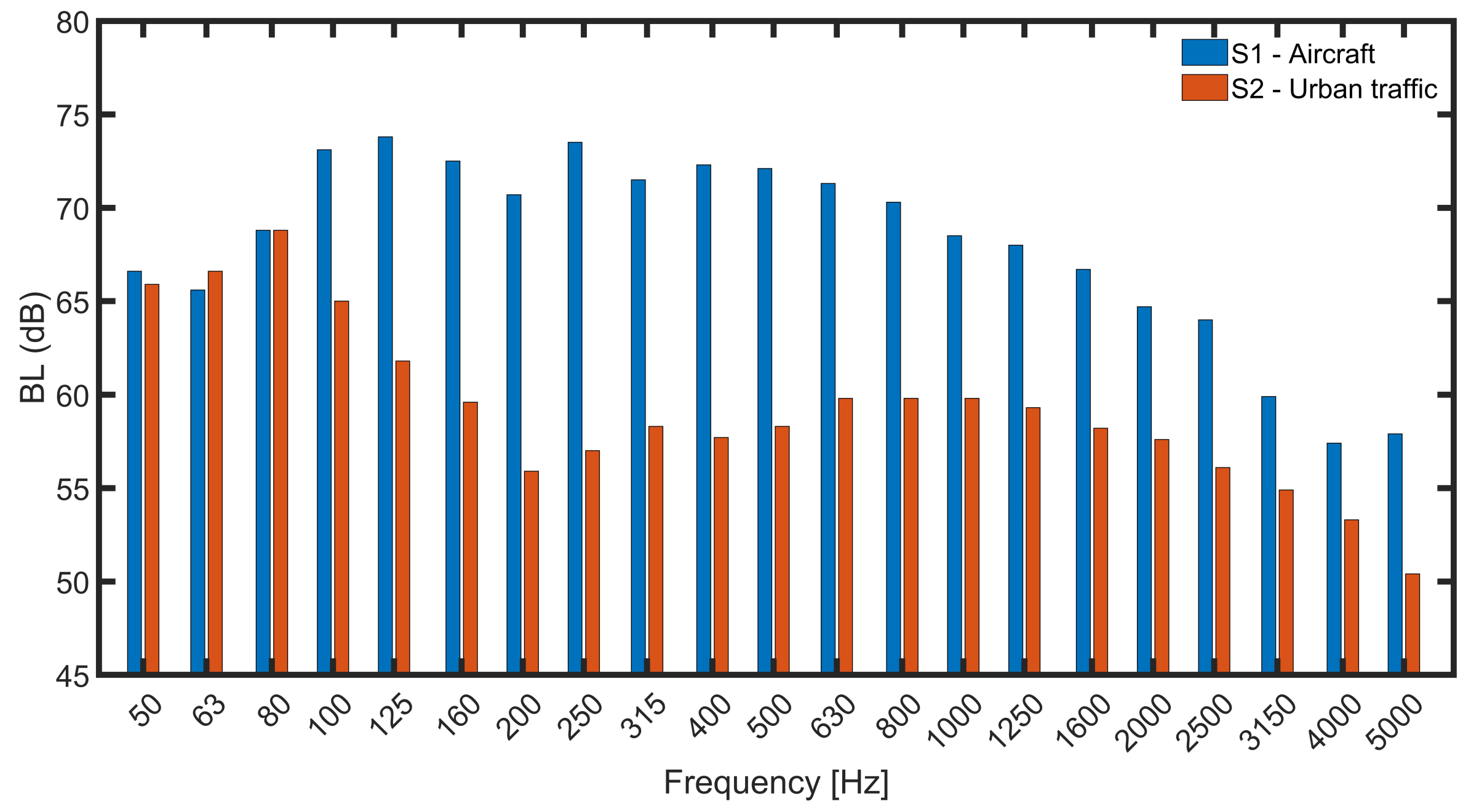
  • Two short-duration urban-type binaural sound samples were selected, from outdoor recordings;
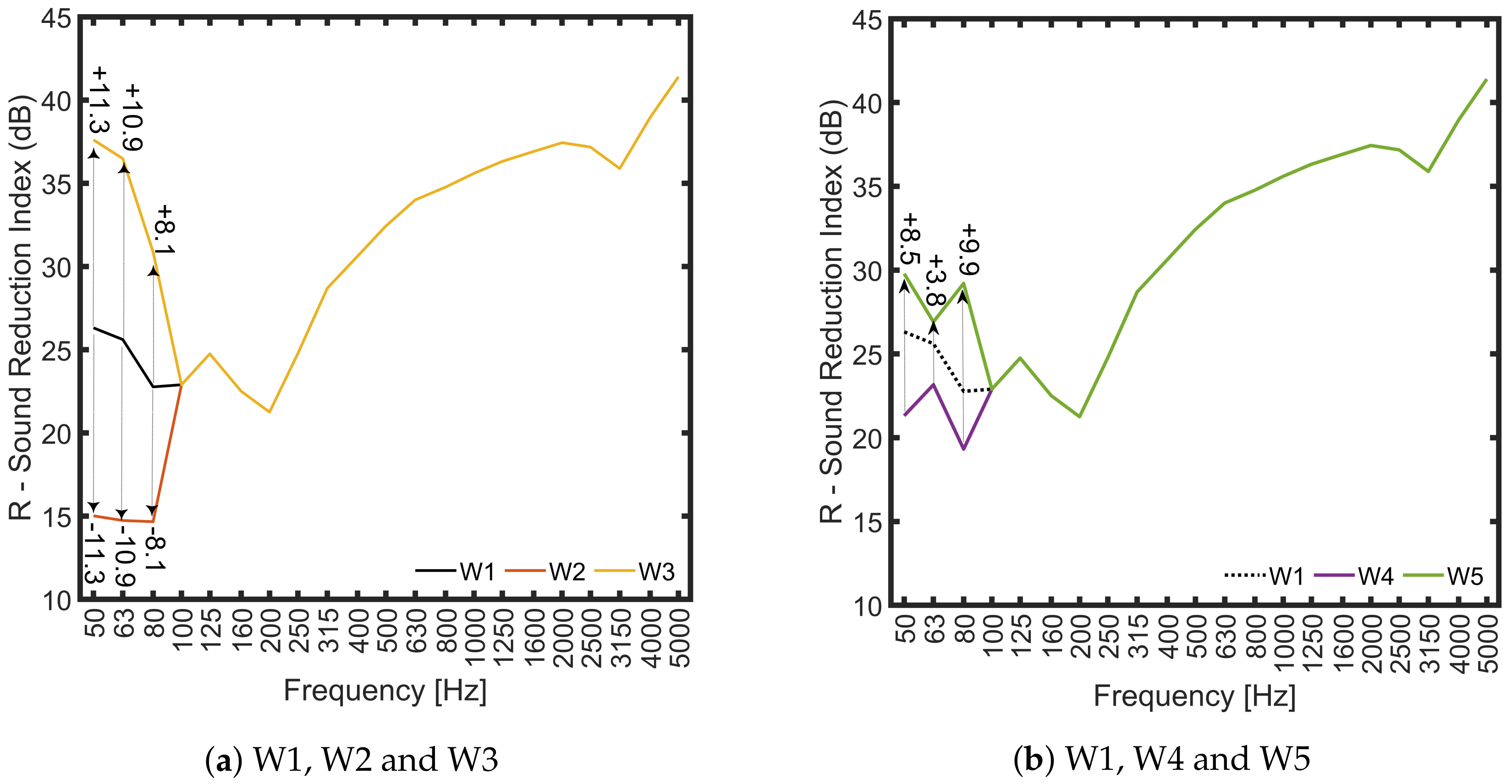
  • These sound samples were processed using filters that mimicked the response provided by nine SRIs obtained in the range [50–5000] Hz, with differing attenuation in the bands of 50, 63, and 80 Hz;
  • The previously filtered signals were additionally processed using a filter with the inverse frequency response of the headphones used during the test, to mitigate the possible influence of the frequency response of the playback device on the assessments.
Figure 2. Schematic illustrating the process followed for the synthesis of the stimuli used during the listening test.
Buildings 13 02561 g002
In this way, 18 binaural audio samples were obtained (i.e., 9 stimuli for each urban-type sound sample), which mimicked the sensation of listening to the urban noises attenuated by the sound insulation of the nine different construction elements. Although in a real-life scenario, the acoustics and background noise of the receiving room could affect the perception, these factors were not considered in the present research. Since no background noise and room characteristics are standardised for this kind of test, the experimenters would have to select them, and this could potentially lead to additional biases and unknowns in the test. Moreover, adding this feature would change the purpose of the study, not only focusing on the perception of sound insulation variations, but also on room characteristics. Consequently, for each sound sample, the only difference between the nine stimuli was their spectral content due to the SRI used. In any case, in Section 4, comments will be made on how these characteristics could affect the results of the perceptual judgements, if they had been taken into account.
The filtering process was carried out using high-order finite impulse response (FIR) filters to accurately replicate the attenuation provided by each SRI, whose spectral information was detailed in 1/3 octaves. The filtering was performed with a bidirectional zero-phase Matlab® filter, to prevent the modification of the phase of the original sound samples in any way.

2.2.1. Selection of the Sound Samples

Considering the purpose of the study, it was important to select representative excerpts of urban-type sounds to be the outdoor sound samples (i.e., Step 1 in Figure 2).
For this purpose, urban sound recording campaigns were carried out in the city of Madrid, including two types of recordings:
  • Fifteen-minute recordings in 13 locations in the city of Madrid, where the main source of noise was mixed traffic (i.e., light, heavy, and motorcycles) with different proportions of vehicle types and road speeds. In some of these locations, several recording sessions were conducted in different weeks.
  • One-hour recordings of aircraft overflights in the vicinity of the Adolfo Suárez Madrid-Barajas airport, on different days. These measurements were carried out in two different urban environments without road traffic and where the main source of noise was aircraft noise.
All of these recordings were taken on days with no adverse weather conditions (i.e., no excessive winds or rain). The recording device was a high-precision B&K Pulse data acquisition device, managed through the Sonoscout® v. 2.0.443 software. This device was connected to a B&K Type 4100-D Dummy Head. The recording format was WAV with a 32 bit resolution and a sampling rate of 96 kHz. More details of the recording methodology and equipment can be found in [44].
From these recordings, a selection of representative excerpts of different urban situations (i.e., traffic at different speeds, pedestrian noise, aircraft noise, etc.) was conducted. This process, which is briefly described below, can be found in schematic format in a previous publication [44]:
  • For each recording location, the averages of the main psychoacoustic indicators [45] (i.e., loudness, sharpness, roughness and fluctuation strength) were computed for the whole recordings. If a recording location was measured in several sessions, the average was then calculated from the averages of each individual recording.
  • Each recording was then divided into small fragments. For the traffic environments, 10 s segments were chosen. For the aircraft environments, we manually extracted each individual aircraft event recorded.
  • The same psychoacoustic indicators were calculated from all of these short excerpts.
  • An automatic selection process was then used to find the fragments with all their psychoacoustic indicators close to those of the complete recordings, within a small range of variability.
  • Although this process may sometimes return only one fragment, often, a small group of samples met the criteria for each location. The final decision on which fragment to use was made by critical listening, avoiding fragments with abrupt beginnings or ends and large fluctuations in level.
Because this robust selection process was based on statistical criteria and highly perceptual psychoacoustic indicators, it provided final sound samples that can be considered good and representative proxies for the usual behaviour of the environments and emitters evaluated.
From the representative fragments, those belonging to low-speed mixed vehicle noise and aircraft overflight were selected. These types of urban noise are among those that normally have the highest prominence of low frequencies and are also relatively frequent. The spectra of the two sound samples are shown in Figure 3, where S1 and S2 refer to the aircraft fragment and the urban traffic excerpt, respectively.
S1 consists of the overflight of a single commercial aircraft at a low altitude of about 1.5 km above the ground, with the recording location about 3 km in a straight line from the end of the runway. The height above ground level was determined during the recording by the B&K Webtrak online monitoring system. This software also provided the aircraft model, which, for this excerpt, belonged to the most-common family of aircraft in [46]. Indeed, the shape of S1’s spectrum is very similar to that of this family [46], albeit at a slightly higher overall level. This, together with the fact that the location was so close to the airport and that the aircraft was in initial climb, made this sample a representative overflight in a high-aircraft-noise environment.
The Dummy Head was placed with its back to the nearest façade and at a distance of at least two meters from it. The overflight took place in front of the Dummy Head at the height described.
Regarding S2, this was a fragment of a low-speed urban traffic (i.e., recorded on a street with a 50 km/h speed limit), consisting of a passing car and the sound of a motorcycle and a delivery van. Its spectra resembled the average of those presented for light urban traffic noises at different speeds in [22], especially at low frequencies. At the location where S2 was recorded, the Dummy Head was with its back to the nearest façade and parallel to the road. The distance from the façade to the back of the Dummy Head was about 2.5 m, with the road in front of the Dummy Head at about 1 m.
The short duration of both sound samples (i.e., 10 s) is important in comparative approaches to reduce the effect that amplitude modulation [35] might have on perception. It is important to note that participants should perceptually evaluate the entirety of the stimuli and not just their beginning or end [22].
Figure 3 shows that both sound samples had very similar band levels (BLs) for the 1/3 octave bands of 50, 63, and 80 Hz (i.e., a difference of 0.7 dB at 50 Hz, 1 dB at 63 Hz, and a negligible difference at 80 Hz), but very different spectral behaviour for the rest. This spectral similarity in the low frequencies was very convenient for the experiment, as it may allow assessing whether the spectral relationship between the low-frequency bands and the adjacent ones in the usual measurement range (i.e., 100–5000 Hz) may have an influence on the perception of low frequencies.

2.2.2. Determination of the SRIs

The determination of the SRIs used to filter the sound samples and construct the test stimuli was based on a statistical study of façade elements commonly used in European construction in recent decades. As the window is usually the worst sound-insulating element in the façade, only window element measurements were considered in this statistical study. Although façades can consist of several elements, such as several windows and the solid wall, we decided to use SRIs from measurements of individual window elements only, in order to avoid the peculiarities of each construction design.
Finally, the SRIs in the range of [50–5000] Hz of 31 elements were collected. These SRIs were obtained from laboratory measurements, following the procedures of ISO 10140-2:2021 [3] and the requirements of the ISO 10140 series of standards regarding transmission chambers, as well as the dimensions and mounting of the tested element. Although many of the SRIs were derived from our own measurements, some were also obtained from building component catalogues and simulation software.
Figure 4 shows the SRIs of each element, as well as the mean and standard deviation of all of them, to allow a visual assessment of the dispersion of the data. However, for the sake of brevity and clarity, Figure 4 does not include legends, nor are tabulated values given, as these SRIs were only used for the statistical study. However, a detailed description of the elements and their Rw is given in Table A1 of Appendix A.
In this sense, since our study focused only on the assessment of low frequencies, the final SRIs used to filter the sound samples did not belong directly to any of the reported spectral curves, but were constructed according to the next statistical procedure:
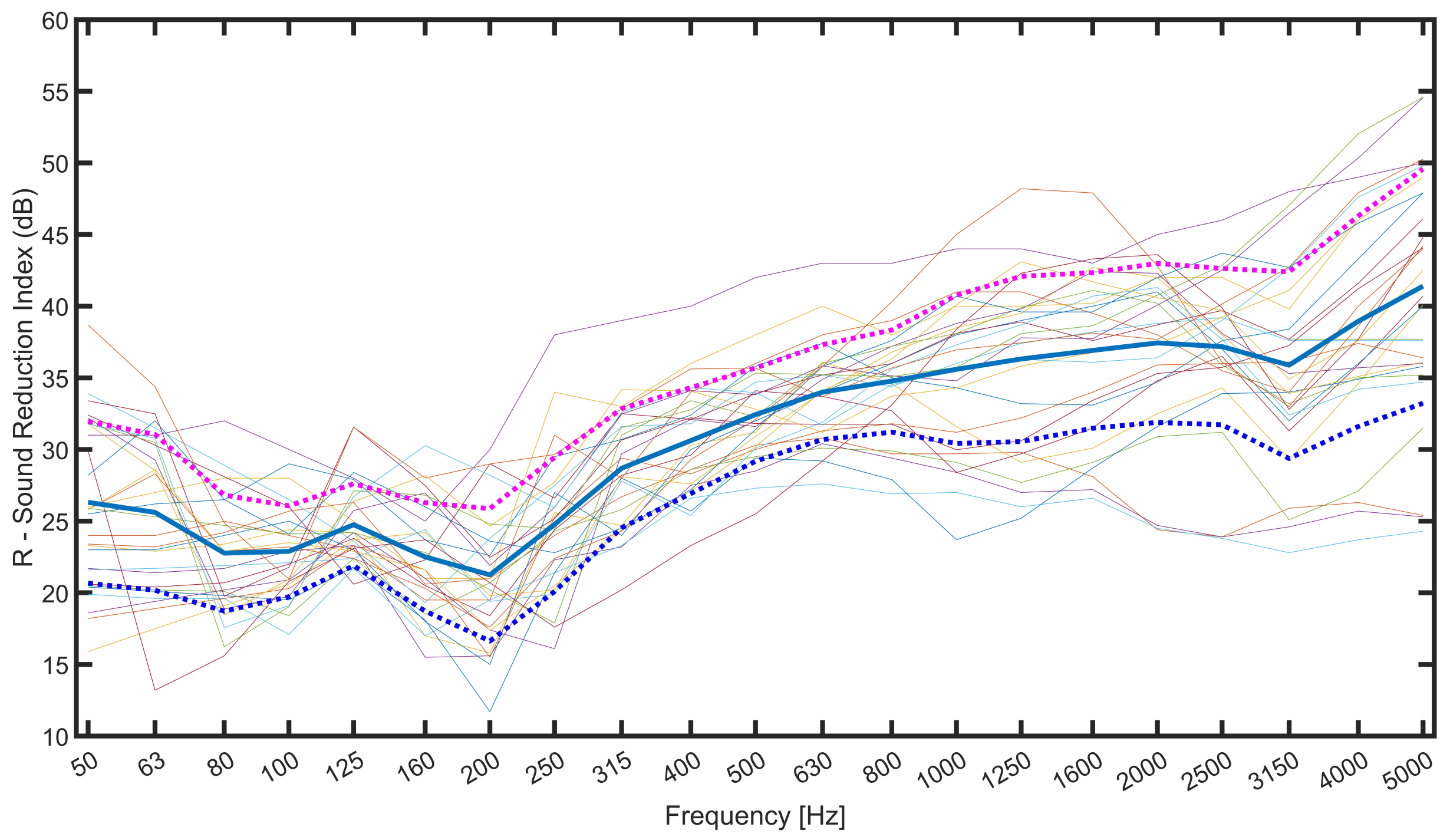
  • The 31 SRIs mentioned were used to calculate the mean and standard deviation of the original dataset (Figure 4), in the range between 50 Hz and 5000 Hz.
  • Using a Monte Carlo approach, 1000 simulated SRIs were obtained, which laid within two standard deviations of the original data (i.e., covering 95% of its variability) for all frequency bands in the range [50–5000] Hz.
  • From these 1000 simulated SRIs, nine were selected: six at random and the other three corresponding to the upper and lower bounds of the Monte Carlo simulations and the mean SRI.
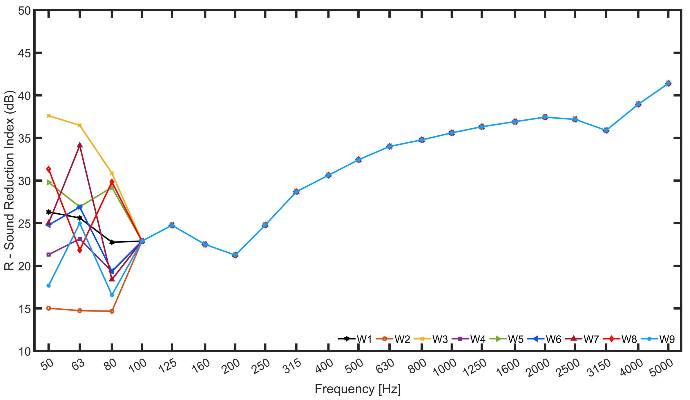
  • The nine finally constructed SRIs had the values of the nine selected SRIs for the frequencies of 50, 63, and 80 Hz, all with the same attenuation (i.e., the values of the average, as shown in Figure 4) from 100 Hz up to 5 kHz. Figure 5 shows the final SRIs, whose specific values, for the low-frequency bands, are given in Table 1. It was considered that the experimenter’s bias was minimal in this process, as the SRIs were chosen randomly, except for the extreme and mean cases.
These final SRIs were used to construct the filters that attenuated the sound samples, to synthesise the listening test stimuli.
It is worth noting that, below the 50 Hz band and above the 5000 Hz band, all the filters applied the same attenuation to the sound samples. These attenuations were those of the mean SRI in the 50 Hz and 5000 Hz bands, respectively. This procedure avoids the potentially drastic action of band-passing the sound samples in the [50–5000] Hz range. In this way, the energy of the sound samples in the remaining frequencies was not excluded, but it was ensured that all stimuli heard during the test, for each sound sample, had the same energy in the frequencies outside the [50–5000] Hz range.
As can be seen from Figure 5 and Table 1, these final SRIs covered a good range of variability in the low-frequency bands, in line with the dispersion of the original data, and although they may not correspond to specific cases, they were considered to provide a detailed perceptual assessment of the effect that variability in the sound insulation over the range of the original data may have on annoyance. In fact, the low-frequency shape of the W4 to W9 elements, with its peaks and valleys, followed the same trend as some of the measurements in the original dataset, as well as those of some of the glazing and window elements presented in [22]. W2 and W3 can be considered as extremes of performance within the range of the original dataset.

2.3. Analysis Methods

2.3.1. Assessment of Discrimination and Perceptual Distance between SRIs

For each pairwise comparison, preference counts were obtained. These represent the total number of participants who, for a given annoyance comparison between two stimuli “A” and “B”, chose each of the three possible answers “A”, “B”, or “No Difference”. From these, discrimination and perceptual distance scores were computed using a specific Thurstonian model fitted for the 2-AC protocol [33,47]. Thurstonian models assume that the intensity of a given attribute of a stimulus can be represented as a probability distribution of the neural input [28]. Therefore, in a trial where two stimuli are compared, a continuous measure of the perceptual difference can be derived from the distance between the two probability distributions. This distance, measured in standard deviations, is known as d . In this sense, d represents how large the perceptual difference between the stimuli is.
Although the size of the difference (i.e., d in Thurstonian models) is considered to be the most-relevant metric in difference testing [48], it is important to perform significance tests to ensure robustly that participants were not simply guessing [48] in a given comparison. Significance tests can be derived from the results of the Thurstonian analysis. The p-value obtained from these tests for all comparisons allowed us to check whether participants actually perceived a clear difference between the stimuli. A threshold of 0.05 was chosen for the p-value (i.e., p-value < 0.05 ), which allowed ensuring a robust perceptual discrimination at a 95% confidence level. Below 0.05, the lower the p-value, the greater the robustness is.
The calculation of the d metric and associated p-value was performed using the R v. 4.0.5 package sensR v. 1.5-1 [49].

2.3.2. Dependence of Preference and Perceptual Distance on the Sound Sample

An independence test was performed to assess whether, for the same comparison, the particular sound sample (i.e., S1 or S2) used during the listening test resulted in a significant change in low-frequency discrimination.
This analysis was considered relevant because S1 and S2 had similar energy contributions in the low-frequency bands, but were very different at higher frequencies and also had different temporal structures. Furthermore, also because the susceptibility of the participants to find certain frequencies more annoying for one or the other type of noise may also be different.
This test of independence could be performed on the listening test data at two different analysis stages: (1) directly on the preference counts, which are discrete and categorical quantities, or (2) on the already-computed d metrics and their standard errors, which are continuous numerical quantities.
The most-appropriate independence test for the two metrics differs, precisely because one metric is categorical (preference counts) and the other is numerical (the value of d ). Probably the best-known independence test, the Student’s t-test, is appropriate when the input data are numerical and continuous [50], whereas the Chi-squared ( χ 2 ) test is more appropriate for discrete and categorical data [30].
Since the calculation of d already involves a transformation of the data obtained during the listening test, it was decided to perform the test of independence directly on the preference counts, and considering that the number of observations was large enough [30], a Chi-squared test was used.
The calculation of the Chi-squared test was performed in Python®, with the help of the Statistics package (scipy). No correction for multiple comparisons (e.g., Holm, Bonferroni, etc.) was applied as only two conditions (i.e., S1 counts vs. S2 counts) were compared.

3. Experimental Setup and Procedure
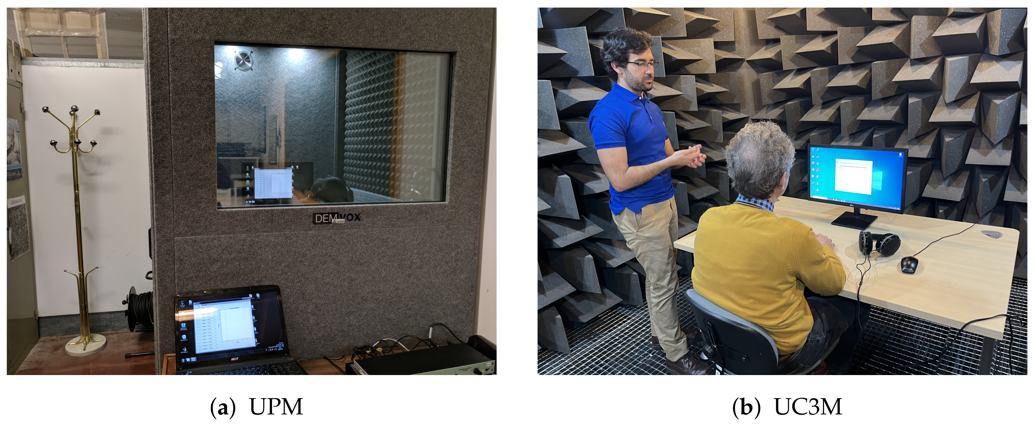
3.1. Environment

The listening test was carried out simultaneously in two different facilities in order to gather as many participants as possible. The first of these was a Demvox Eco100 soundproof booth (Figure 6a) located at the Escuela Técnica Superior de Arquitectura of the Universidad Politécnica de Madrid (UPM). The second (Figure 6b) was the anechoic chamber at the Escuela Politécnica Superior of the Universidad Carlos III de Madrid (UC3M).
Although there were two test facilities, their characteristics were very similar. Both venues were very quiet and had extremely low reverberation times. In fact, in the [50–5000] Hz frequency range, the background noise in both rooms was generally below the ISO 389-7:2019 [51] hearing threshold, with some bands very slightly above it.
In addition to their acoustics, the lighting and colour of the wall coverings in both rooms were neither excessive nor obtrusive, creating a rather neutral visual experience.

3.2. Hardware and Calibration

Participants’ responses should focus solely on their assessment of the quality or qualities being evaluated, i.e., their perception of annoyance associated with variations in low-frequency attenuation. For this to be the case, it is important that the playback system faithfully reproduces the designed signals.
Given that the stimuli were binaural, the simplest way to reproduce them faithfully was through headphones. In particular, two identical pairs (i.e., one for each evaluation room) of Sennheiser HD-650 open circumaural headphones were used. These had been used for approximately the same number of hours prior to the experiment, so their performance was very similar. This model of headphone was chosen because of its standard wide spectral flatness and also because of its openness, which minimises the likelihood of significant variations in the low-frequency range due to the effect of spectral leakage as a result of head fit [52]. The only drawback to using this type of open headphone is that the test room must be extremely quiet. As mentioned above, this condition was met due to the low background noise of both test enclosures.
These headphones were connected to a computer running the DiTAA toolbox [43] via two similar audio interfaces (i.e., an RME Fireface UFX interface at UPM and an RME Fireface UFX-II interface at UC3M) connected to two similar headphone amplifiers (i.e., RANE HC6S at UPM and ART Headamp 6 Pro at UC3M).
Both systems were calibrated with a sinusoidal signal of 1000 Hz and 94 dB, recorded with the same binaural recording system and configuration used for the outdoor recordings. The headphones were attached to the Dummy Head, and the described sound was played. The volume presented in the headphones was adjusted until the level measured by the Dummy Head reached 94 dB. Given that the test stimuli had been processed to correct for the headphone effect, as described in Section 2.2, calibration with a single frequency tone was considered sufficient. In this way, the levels heard by the participants during the test, at the frequencies of interest, were very similar to those they would hear in a very silent dwelling protected from the outside by structural elements with SRIs, such as those used in the test.
To further minimise the noise generated by the electronic equipment used in the test (e.g., computers, audio interfaces, headphone amplifiers, etc.), all this equipment was placed outside the test rooms. These included only the aforementioned headphones, a screen, and a mouse to operate the test computer, which was located outside the test environment.

3.3. Participants

Participants from a variety of backgrounds and professions were recruited by word of mouth. While some had participated in other perceptual studies in the past, most were naïve to listening tests and the specific subject of the research. The participants were not aware of the purpose of the study before it was carried out.
In total, the judgements of 100 participants were used to extract and analyse the results of the experiment. Of these 100 participants, 46 were female and 54 were male. The extreme ages of the participants were 15 and 75 years.
The test was completed by 69 participants at UPM and 31 participants at UC3M. In Section 4, the results are pooled, taking into account the assessments of all 100 participants. However, a preliminary analysis was carried out to ensure that the results were not significantly different in the two settings. This test, which is not shown in the manuscript for ease of reading, reported that there were no significant differences in the judgements derived from the evaluation location, as was expected at the design stage of the experiment.

3.4. Procedure

The following steps were taken in the experimental procedure:
  • Each assessor was received in the test environment on a pre-arranged day and time.
  • The test environment was then shown to the participant, who was then asked to fill in a short questionnaire about his/her age, gender, and professional background. This also helped the assessors become visually and aurally accustomed to the test environment.
  • The participant was given a document describing the test, its protocol, its stages, and other details. This was done to avoid excessive interaction between the experimenter and assessor.
  • A short training session of two comparisons was then carried out in accordance with the test protocol using dummy samples.
  • The test began once the training had been completed without incident and there were no more doubts.

4. Results

4.1. Discrimination and Perceptual Distance between SRIs

The results of perceived discrimination and preference are presented in Table 2, in terms of the measure of perceptual distance, d . In addition, the standard error ( S E ) of d is given for each comparison, as well as the significance of the perceptual difference through the p-value. For the sake of simplicity and clarity, Table 2 only shows the results for those comparisons where the differences between stimuli were significant for both sound samples. The complete Table A2, with data for all comparisons, is shown in Appendix B.
Since the protocol used was intended not only to quantify the perceptual distance between the pairs of stimuli, but also to indicate which was more annoying (i.e., the preference), the d were intended to indicate not only the perceptual distance between the stimuli, but also the direction of the choice. Thus, negative values of d indicate that the first stimulus in a comparison was chosen as the most-annoying. Conversely, positive values of d show that the second stimulus was perceived as more-annoying. The perceived distance between the stimuli is the absolute value of d .
As can be seen in Table 2, the difference in annoyance between the stimuli was significant for both sound samples in 14 of the 36 comparisons made. Inspection of the p-values in Table 2 shows that the judgements of the assessors were very robust. For these 14 comparisons and for both the S1 and S2 sound samples, it can be concluded that the participants perceived a clear difference between the stimuli and were, therefore, able to make a robust judgement about which stimulus was more-annoying. Although the p-values marked with a star are the most-robust (i.e., p-value 0.0001 ), all p-values in Table 2 are below the threshold of p-value 0.05 . For the rest of the comparisons in Table A2, cases where p-value > 0.05 mean that participants could not perceive a clear difference between the stimuli.
Interestingly, of the only 14 comparisons where participants perceived a clear and robust difference, 8 were comparisons of W2 against all others. This SRI, as shown in Figure 5, is the one with the lowest attenuations in the 50, 63, and 80 Hz bands. Furthermore, looking at the direction of the term d , it can be seen that on, all these occasions, the stimulus filtered by W2 was chosen as the most-annoying. This fact is indeed relevant, as it shows that participants were able to perceive and identify the worst SRI (i.e., W2) when it was compared to the others.
Most of the remaining comparisons in Table 2 (i.e., W1–W9, W3–W9, W5–W9, and W8–W9) for which the p-value was significant for both sound samples are mainly related to those comparing W9 with the rest. With the exception of the aforementioned W2, W9 had the lowest SRI values for the 50 and 83 Hz bands.
Some other interesting results can be extracted by analysing Table 2, together with the graphs shown in Figure 7a,b below.
As can be seen in Figure 7a, the difference in low-frequency sound insulation between the SRI of W1 (i.e., average sound insulation) and those of W2 (minimum insulation) and W3 (maximum insulation) is the same and large, averaging 10.1 dB. In Table 2, it can be seen that the W1–W2 comparison produced a significant perceptual change in the participants for both sound samples, with W2 being perceived as more-annoying. However, the W1–W3 comparison does not appear in the table because the participants did not perceive significant differences between W1 and W3 for either sound sample. In fact, it can be seen from Table A2 that the difference for the W1–W3 comparison was not significant for either sound sample. Therefore, it seems that the perception of annoyance does not only depend on the absolute difference in sound insulation, but also on its direction, as expected.
Finally, the perceptual characteristics of the W4–W5 comparison, which remains to be mentioned from Table 2, were analysed in conjunction with Figure 7b. As can be seen from the figure, W5 represents an average improvement of 7.4 dB over W4 in the low-frequency range. Although this increase is smaller on average than that observed between W1 and W3 in Figure 7a, this difference between W4 and W5 does in fact lead to a significant perceptual difference in terms of annoyance for the participants.
Considering all comparisons, the results seem to indicate that participants were mostly able to perceive a clear difference between stimuli only in those comparisons where one of the cases matched with SRIs worse or much worse than the average sound insulation. Therefore, except in somewhat extreme situations, low-frequency variations in sound insulation were generally not detected by the participants.

4.2. Effect of Sound Samples on the Perceptual Judgements

The participants performed the same experiment twice, once for each of the sound samples S1 and S2. As mentioned in Section 2.2, they had similar energy in low frequencies, but very different spectral content in the upper bands adjacent to the low frequencies. For this reason, it seems interesting to evaluate whether these differences led to a different perception at low frequencies by the participants.
The results of the Chi-squared ( χ 2 ) test enabled determining whether, for the same comparison, but different sound samples, the number of participants selecting “A”, “B”, and “No Difference” varied significantly.
Given the large number of comparisons (i.e., 36) and to simplify the presentation of the results, these are shown in Figure 8 as a bar chart rather than in tabular form.
Figure 8 shows the p-value of the Chi-squared ( χ 2 ) test for each of the 36 comparisons (i.e., W1–W2, …, W8–W9), the p-value considering all comparisons together (“pooled” in Figure 8), as well as the significance threshold, which was set at the usual p-value < 0.05 .
As can be seen from the pooled data, with a p-value = 0.89, it appears that participants did not perceive the same comparisons significantly differently depending on the sound sample used. Although this was partly to be expected given the similar spectral content of S1 and S2 at low frequencies, it allowed us to verify that, in general, the temporal structure of these two sounds and their different behaviour at upper adjacent frequencies did not cause major changes in the judgements.
There were only two cases, W1–W4 (Figure 9a) and W2–W7 (Figure 9b), where the p-value was less than 0.05, slightly below and above p-value = 0.02, respectively.
The low-frequency difference between W1 and W4 was small, about 3.6 dB on average, as can be seen from Figure 9a. Looking further at Table A2, we can see that, for this comparison, d was very low in absolute value (i.e., close to 0) and that the p-value was not significant for either sound sample in the W1–W4 comparison, meaning that participants were not able to perceptually distinguish between W1 and W4 for either S1 or S2. It is likely that the significant changes in participants’ judgements between S1 and S2 found by the Chi-squared test for this comparison (see Figure 8) were not related to a real perceptual change, but rather to participants’ guessing, indistinctly marking one or the other stimulus as more-annoying in the face of a difference in sound insulation that did not evoke a significant perceptual change in them.
For the case W2–W7 (Figure 9b), the scenario was different. In this case, the difference in sound insulation at low frequencies between W2 and W7 was about 11.0 dB on average, with a large difference of 19.4 dB in the 63 Hz band. In fact, Table 2 shows large d values and extremely low p-values for both S1 and S2. However, these d values were very different, being (based on the Chi-squared analysis) significantly higher for S1 than for S2. The higher spectral content of S1 at frequencies adjacent to the low frequencies (e.g., 100 Hz, 125 Hz, etc.) could make the strong attenuation of the 63 Hz band of W7 relative to W2 more noticeable to the ear for the S1 sound sample than for S2.

5. Discussion

5.1. Overall Discrimination of the Low Frequencies

This study made it possible to assess whether a sample of assessors was able to detect differences between stimuli that differed only in their low-frequency spectral content, by simulating the attenuation caused by different elements with the same SRIs in the range between 100 and 5000 Hz, but different for the 50, 63, and 80 Hz bands. If the participants perceived a significant difference, the study was also used to quantify this difference. The experiment was repeated for two different urban sound samples, relating to urban mixed traffic noise and aircraft overflight noise, using highly representative samples.
This evaluation showed that participants were generally unable to discriminate between stimuli consisting of the same sound sample, but with different energy at low frequencies, due to variations in sound insulation within the range expected for window façade elements typical of European construction in recent decades. This can be seen from the fact that, in only 14 of the 36 comparisons that were carried out, did the participants perceive a significant difference between the stimuli for the two sound samples that were used. In the remaining comparisons, in view of Table A2, participants were unable to distinguish clearly between the stimuli for at least one of the two sound samples, and usually for both. Moreover, the comparisons in which they were able to perceive significant differences were mainly those in which the sound samples were filtered with the SRIs of W2 and W9 and compared with the rest. These two SRIs, especially W2, were examples of very low attenuation at low frequencies. Although both were within the expected sound insulation values for windows, they were cases of poor acoustic performance in view of the statistical study carried out on window elements of façades.
The results of this research, which focused exclusively on the study of low frequencies, were in line with research in the same field. In this sense, it was found that, as concluded in [15,22,27], in general, the sound insulation of façade elements is not particularly relevant at low frequencies, since usually no significant differences are perceived by assessors with attenuation changes in this range. Therefore, for sound insulation characterisations using the currently standardised SNQs, ranges from 100 Hz could be used as a good compromise.
This does not detract from the fact that, for some particularly poor, but still statistically possible, sound insulation conditions (such as those of W2 and W9 in the current study), changes in the low frequencies may be detectable and, therefore, relevant, and better SNQs could be computed that also take these cases into account. In this sense, it was considered that research similar to [20] should be carried out, taking into account more types of urban noise and sound insulation cases, in order to define robust reference curves starting from 50 Hz that allow the calculation of perceptually better SNQs than those currently standardised. In this way, these new SNQs could take into account, in addition to the more-general sound insulation behaviour of façades, specific scenarios such as poor, but statistically possible sound insulation in the 50, 63, and 80 Hz bands.

5.2. Influence of the Sound Sample

In this research, the perception of low-frequency variations in sound insulation was evaluated for two different urban sound samples whose characteristics belong to common cases of urban noise. In particular, an overflight of a commercial aircraft (S1), belonging to the most-common family of aircraft in Europe, and a highly representative sample of mixed urban traffic noise at low speeds (S2), which was considered to render well the overall traffic soundscape in cities, were used.
Interestingly, these two sound samples had very similar spectral behaviour and band levels for the 50, 63, and 80 Hz bands, so no significant perceptual changes between the low frequency detectability of one sound sample and the other would be expected.
Nevertheless, a statistical analysis was carried out to determine whether other factors could cause a significant change in the discrimination of the low frequencies, such as the different temporal structure of the sound samples, the susceptibility of the listeners to different types of sound (i.e., traffic vs. aircraft), or the energetic content in the upper adjacent bands to the low-frequency range.
In general, the results showed that these factors had no significant effect on the ability to detect changes in the low frequencies and the perception of annoyance, with the similar energy content of both sound samples at low frequencies being the most-relevant factor. This fact showed, as expected, that the low-frequency energy of the sound incident on the façades seems to be more relevant to the annoyance that these frequencies can cause in humans than the susceptibility to a specific type of sound or its temporal evolution.
In view of this result, it is to be expected that, for other types of urban noise that are less frequent, but have a higher low-frequency content, such as heavy traffic noise, construction work, or alarms, the detection of these frequencies and their impact on annoyance may be higher. This fact has already been highlighted in previous research [22], where it was shown that low frequencies can be relevant for the characterisation of sound insulation in heavy-traffic-noise conditions.
It is, therefore, considered necessary to carry out further similar research with different types of urban noise in order to adequately characterise the influence of low frequency for as many realistic cases as possible.

5.3. Influence of the Experimental Design

This study was conducted using open headphones (i.e., without attenuation) in very quiet environments. The background noise in these test rooms was below or very close to the hearing threshold in all bands of interest. It is, therefore, believed that the low-frequency discrimination results may be similar to those expected in real-life situations with very low background noise, for example in homes at night. However, for other background noise conditions (e.g., typical residential background noise in the day-time period), it would be expected that some of the comparisons in which participants were able to detect low-frequency differences would not result in a noticeable difference due to background noise masking.
Furthermore, the test stimuli were constructed only by filtering the sound samples with filters simulating different sound insulation attenuations. Therefore, the possible influence of the receiving room on the low frequencies and their detectability was not taken into account. It is to be expected that the detection and annoyance of low frequencies will vary with the type of receiving room and the position of the listener. This may be particularly relevant in some scenarios, such as bedrooms. In bedrooms, the bed is sometimes placed close to the corners, where the modal behaviour enhances low frequencies. If this enhancement is added to possible situations with low background noise, such as a resting at night scenario, the detectability and influence of low frequencies could be greater, increasing annoyance.
Finally, it should be noted that both the sound samples and the SRIs used to attenuate them were selected based on statistical analysis to reduce bias as much as possible and to select particularly representative cases. However, this does not change the fact that other research with the same purpose may result in different sound samples for the same types of noise and other representative SRIs with slightly different acoustic characteristics. In these situations, the detection of low frequencies may vary.

6. Conclusions and Future Lines of Research

The research assessed, by means of a listening test, the detectability and annoyance of low-frequency variations in the sound insulation of façade window elements, within the expected range of variation based on a statistical study of window elements commonly used in European construction. This evaluation allowed conclusions to be derived for two urban noise samples, related to the noise of a commercial aircraft overflight and mixed urban traffic at low speeds.
It was observed that, in general, the detectability of variations at low frequencies and the change in perceived annoyance were limited for the sound samples used and for low-frequency sound insulation variations in the range predicted for window elements.
It was observed, however, that, for situations with poor sound insulation, low-frequency variations in sound insulation may be clearly detectable and elicit a change in perceived annoyance.
These results suggested that expressing the façade sound insulation in the case of windows by SNQs calculated from 100 Hz would be sufficient in most situations, as the discrimination of low frequencies was limited. However, given the detectability of low-frequency changes and the increased annoyance observed with poor sound insulation conditions, further similar experiments using other plausible types of sound samples and variations in sound insulation are strongly recommended. The data obtained from this and further research could be used to provide new and better reference curves for the calculation of perceptually relevant SNQs, starting at 50 Hz. These could be representative not only of the most-common scenarios, but also of special cases within the range of variation in façade sound insulation and expected outdoor noise levels.
In this sense, the future lines of this research by these authors include further perceptual evaluation, with other conditions and factors, to increase the dataset of annotated perceptual judgements. It is hoped that, with the results of past, current, and future research, these authors can soon apply robust machine and deep learning techniques to draw further conclusions.

Author Contributions

Conceptualisation, D.d.l.P., M.Á.N., A.P. and L.A.A.-R.; methodology, D.d.l.P.; software, D.d.l.P.; validation, D.d.l.P., L.A.A.-R., M.Á.N. and A.P.; formal analysis, D.d.l.P.; investigation, D.d.l.P., M.A.-Y., D.C. and M.Á.N.; resources, M.Á.N., D.C., D.d.l.P. and L.A.A.-R.; data curation, D.d.l.P. and M.A.-Y.; writing—original draft preparation, D.d.l.P.; writing—review and editing, D.d.l.P., L.A.A.-R., M.Á.N. and D.C.; visualisation, D.d.l.P.; supervision, M.Á.N., L.A.A.-R. and A.P.; project administration, M.Á.N.; funding acquisition, M.Á.N. All authors have read and agreed to the published version of the manuscript.

Funding

This research was supported by Grant RTI2018-094656-B-I00 funded by MCIN/AEI/10.13039/501100011033 and by the European Union “ERDF A way of making Europe”. The work of de la Prida and Azpicueta-Ruiz was also partly supported by Grants TED2021-130909A-I00 and PID2021-124280OB-C21 funded by MCIN/AEI/10.13039/501100011033 and by the European Union NextGenerationEU/PRTR and “ERDF A way of making Europe”.

Informed Consent Statement

Informed consent was obtained from all subjects involved in the study.

Data Availability Statement

The data presented in this study are available on request from the corresponding authors.

Acknowledgments

The authors would like to thank all the participants in the experiment for their willingness, dedication, and time in carrying out the test.

Conflicts of Interest

The authors declare no conflict of interest. The funders had no role in the design of the study; in the collection, analyses, or interpretation of the data; in the writing of the manuscript; nor in the decision to publish the results.

Abbreviations

The following abbreviations are used in this manuscript:
SNQ Single-number quantity
2-AC Two-Alternative Choice
DiTAA Difference Testing in Architectural Acoustics
FIR Finite impulse response
BL Band level
SRIs Sound reduction indices
2-AFC Two-alternative forced choice
SRI Sound reduction index
CDS Cognitive decision strategy
SDT Signal-detection theory
UPM Universidad Politécnica de Madrid
UC3M Universidad Carlos III de Madrid

Appendix A. Detailed Description of the Window Elements Used for the Statistical Study

Table A1 presents the main characteristics of the window elements whose SRIs were used for the statistical analysis. This table includes data about the window, such as the frame material, the opening arrangement, or the presence of a shutter box, as well as details about the glazing used, such as whether it was single or multi-pane and the glass thicknesses. Finally, the Rw of each element is also given. The SRIs from the laboratory measurements of these elements are the thin lines shown for reference in Figure 4, along with the mean and standard deviation.
Table A1. Rw and overall description of the features and glazing of each of the window elements used for the statistical study.
ElementRwGlazingWindow Description
E1334/12 Air/4PVC window Kömerling Eurodur 1 leaf vertical and horizontal casement
E2344/12 Air/4PVC window Kömerling Eurodur 1 leaf vertical and horizontal casement
E3294Traditional aluminium window horizontal sliding 2-wing
E4354/12 Air/10Traditional aluminium horizontal casement window 2-leaf
E5284/12 Air/10Traditional aluminium vertical casement
E6368/14 Air/8Wooden window SIA “Eiger”, 2-leaf casement window
E7334/12 Air/4PVC window Rehau Euro 70 with roller shutter box, horizontal 2-leaf casement
E8314/16 Air/4Traditional aluminium window, 2-leaf casement window
E9344/16 Air/4Standard PVC window horizontal casement window 2-leaf
E10364/16 Air/6Standard PVC window horizontal casement window 2-leaf
E11364/12 Air/8PVC window Rehau Euro 70 with roller shutter box, horizontal 2-leaf casement
E12324/16 Air/4Traditional wooden window, 2-leaf casement window
E13364/14 Air/8Wooden window Wenger Holzfenster Eiger
E14264Traditional aluminium vertical casement
E15354/12 Air/33.1PVC window Rehau Euro 70 with roller shutter box, horizontal 2-leaf casement (retracted shutter)
E16364/12 Air/33.1PVC window Rehau Euro 70 with roller shutter box, horizontal 2-leaf casement (extended shutter blind)
E17274/16 Air/4Traditional aluminium vertical casement
E18324/12 Air/4PVC window Kömerling Premiline horizontal sliding 2-wing
E19378/12 Air/8PVC window Rehau Euro 70 with roller shutter box, vertical and horizontal 2-leaf casement
E20384/16 Air/10Standard PVC window horizontal casement window 2-leaf
E21374/12 Air/44.1PVC window Rehau Euro 70 with roller shutter box, horizontal 2-leaf casement (retracted shutter)
E22364/12 Air/44.1PVC window Rehau Euro 70 with roller shutter box, horizontal 2-leaf casement (extended shutter blind)
E234344.2/16 Air/10Standard PVC window horizontal casement window 2-leaf
E24364/16 Air/8Aluminium window horizontal sliding 2-wing
E25354/12 Air/4PVC window Kömerling Eurodur 2-leaf vertical and horizontal casement
E26284/12 Air/4PVC window Kömerling SF3 horizontal sliding 2-wing
E27344/12 Air/4PVC window Kömerling Eurodur 1-leaf vertical and horizontal casement
E28314/12 Air/4PVC window Rehau Euro 70 with roller shutter box, horizontal 2-leaf casement
E29368/12 Air/4PVC window Rehau Euro 70 with roller shutter box, horizontal 2-leaf casement
E30344/16 Ar/44.1PVC window Rehau Euro 70 with roller shutter box, horizontal 2-leaf casement
E31334/12 Air/33.1PVC window Rehau Euro 70 with roller shutter box, horizontal 2-leaf casement

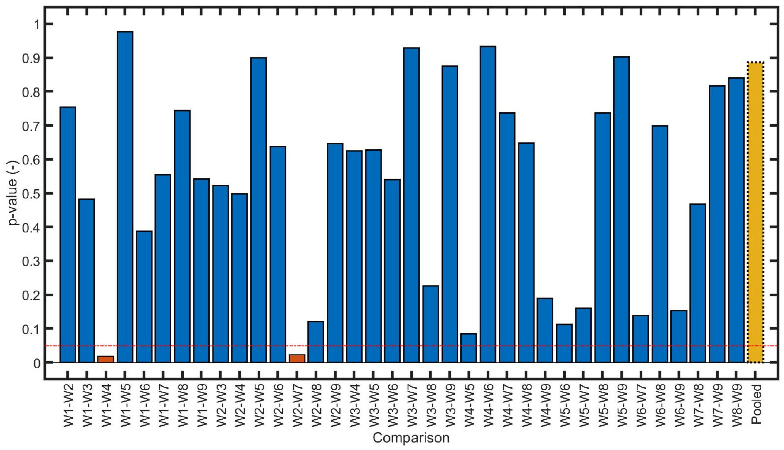
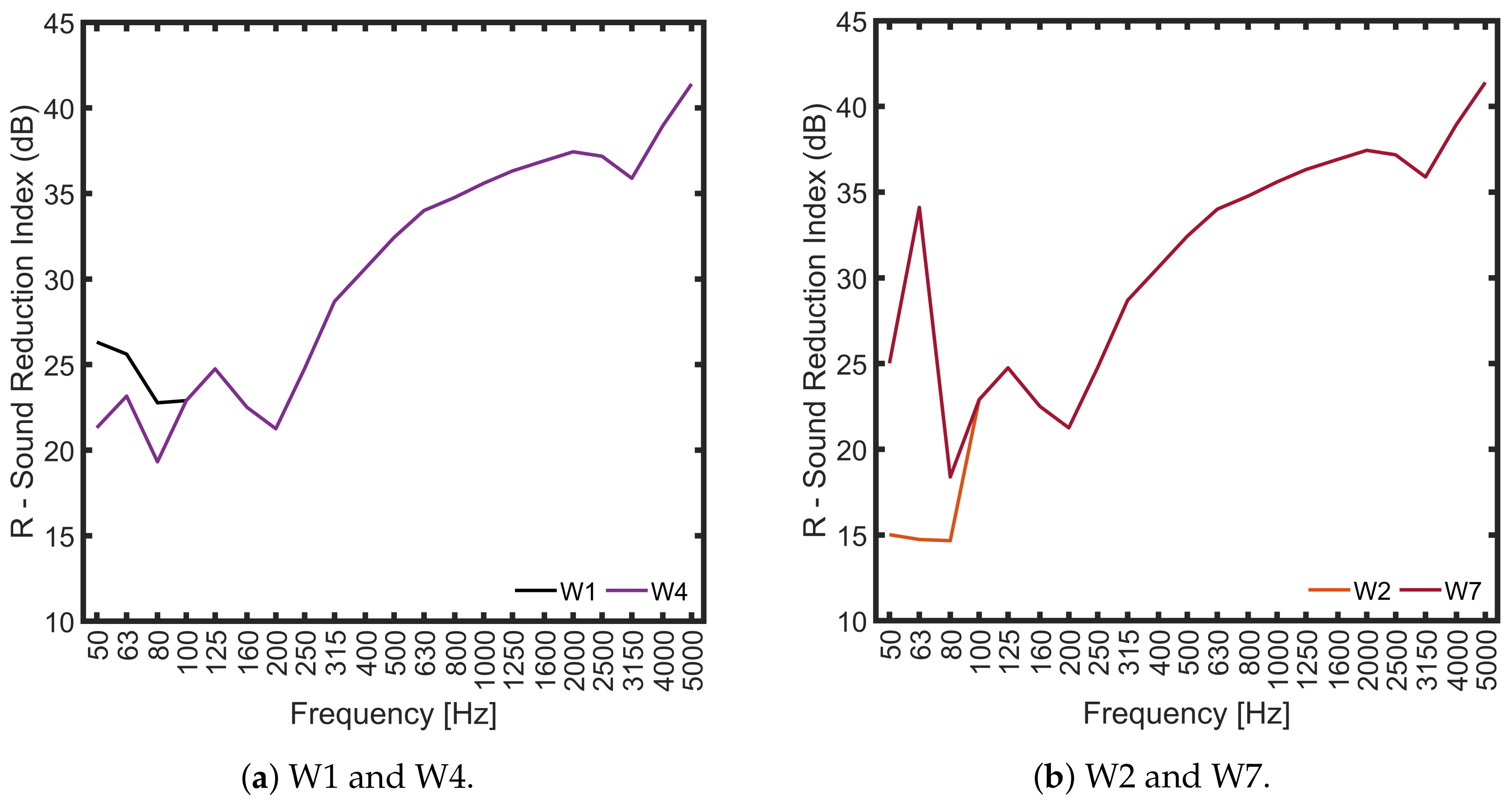
Appendix B. Perceptual Difference in All Comparisons

This Appendix presents the d values, their standard error ( S E ) , as well as the significance of the difference, through the p-value, for each of the comparisons made by the participants, for both the S1 and S2 sound samples. In this sense, Table A2 can be understood as a complete version of Table 2, including not only the comparisons where the result was significant for both sound samples, but rather all the comparisons made.
Table A2. d ( S E ) and p-values for each of the comparisons performed by the participants during the test. Results presented for both sound samples (i.e., S1—aircraft; S2—urban traffic).
d ( SE )   ap-Value b
ComparisonS1S2S1S2
W1–W20.92 (0.19)1.03 (0.19)
W1–W3−0.33 (0.17)−0.07 (0.17)--
W1–W4−0.05 (0.17)0.13 (0.16)--
W1–W50.07 (0.17)0.13 (0.17)--
W1–W6−0.18 (0.17)0.09 (0.17)--
W1–W70.53 (0.18)0.29 (0.17)**-
W1–W8−0.22 (0.17)−0.18 (0.17)--
W1–W90.61 (0.18)0.34 (0.17)****
W2–W3−1.02 (0.19)−0.73 (0.18)
W2–W4−0.90 (0.19)−0.83 (0.18)
W2–W5−0.77 (0.18)−0.85 (0.18)
W2–W6−0.57 (0.18)−0.81 (0.18)**
W2–W7−1.15 (0.21)−0.73 (0.18)
W2–W8−0.44 (0.17)−0.72 (0.18)*
W2–W9−0.46 (0.18)−0.68 (0.18)*****
W3–W40.27 (0.18)0.34 (0.17)-*
W3–W50.37 (0.17)0.18 (0.17)*-
W3–W60.33 (0.17)0.57 (0.18)-**
W3–W70.53 (0.18)0.49 (0.18)****
W3–W80.07 (0.17)0.25 (0.17)--
W3–W90.86 (0.18)0.76 (0.18)
W4–W5−0.68 (0.17)−0.49 (0.18)**
W4–W6−0.22 (0.17)−0.29 (0.17)--
W4–W7−0.05 (0.17)−0.23 (0.17)--
W4–W8−0.35 (0.17)−0.23 (0.17)*-
W4–W90.29 (0.17)−0.14 (0.17)--
W5–W6−0.02 (0.17)0.47 (0.17)-**
W5–W70.07 (0.17)0.50 (0.17)-**
W5–W80.02 (0.17)0.20 (0.17)--
W5–W90.50 (0.18)0.42 (0.17)***
W6–W70.16 (0.17)−0.18 (0.17)--
W6–W8−0.50 (0.18)−0.30 (0.17)**-
W6–W90.21 (0.17)0.36 (0.17)-*
W7–W80.22 (0.17)−0.07 (0.17)--
W7–W90.22 (0.17)0.07 (0.17)--
W8–W90.42 (0.17)0.36 (0.17)**
a Considering the 2-AC preference task, absolute values of d represent the perceptual distance and the sign of the difference the direction. Negative signs indicate more annoyance for the first item, the opposite for positive signs. b For the sake of simplicity, p-values are shown as follows: p-value > 0.05 (-); 0.01 < p-value 0.05 (*); 0.001 < p-value 0.01 (**); 0.0001 < p-value 0.001 (***); p-value 0.0001 (★).

References

  1. ISO 16283-1:2014; Acoustics—Field Measurement of Sound Insulation in Buildings and of Building Elements—Part 1: Airborne Sound Insulation. International Organization for Standardization: Geneva, Switzerland, 2014.
  2. ISO 16283-3:2016; Acoustics—Field Measurement of Sound Insulation in Buildings and of Building Elements—Part 3: Façade Sound Insulation. International Organization for Standardization: Geneva, Switzerland, 2016.
  3. ISO 10140-2:2021; Acoustics—Laboratory Measurement of Sound Insulation of Building Elements—Part 2: Measurement of Airborne Sound Insulation. International Organization for Standardization: Geneva, Switzerland, 2021.
  4. ISO 717-1:2020; Acoustics— Rating of Sound Insulation in Buildings and of Building Elements—Part 1: Airborne Sound Insulation. International Organization for Standardization: Geneva, Switzerland, 2020.
  5. Yaniv, S.L.; Flynn, D.R. Noise Criteria for Buildings: A Critical View; Special Publications; National Bureau of Standards: Washington, DC, USA, 1978; Volume 499. [Google Scholar]
  6. Vardaxis, N.G.; Bard, D. Review of acoustic comfort evaluation in dwellings: Part III—Airborne sound data associated with subjective responses in laboratory tests. Build. Acoust. 2018, 25, 289–305. [Google Scholar] [CrossRef]
  7. Vian, J.P.; Danner, W.F.; Bauer, J.W. Assessment of significant acoustical parameters for rating sound insulation of party walls. J. Acoust. Soc. Am. 1983, 73, 1236–1243. [Google Scholar] [CrossRef]
  8. Park, H.K.; Bradley, J.S.; Gover, B.N. Evaluating airborne sound insulation in terms of speech intelligibility. J. Acoust. Soc. Am. 2008, 123, 1458–1471. [Google Scholar] [CrossRef]
  9. Park, H.K.; Bradley, J.S. Evaluating standard airborne sound insulation measures in terms of annoyance, loudness, and audibility ratings. J. Acoust. Soc. Am. 2009, 126, 208–219. [Google Scholar] [CrossRef]
  10. Rychtáriková, M.; Roozen, B.; Müllner, H.; Stani, M.; Chmelík, V.; Glorieux, C. Listening test experiments for comparisons of sound transmitted through light weight and heavy weight walls. Akustika 2013, 19, 8–13. [Google Scholar]
  11. Hongisto, V.; Oliva, D.; Keränen, J. Subjective and objective rating of airborne sound insulation–living sounds. Acta Acust. United Acust. 2014, 100, 848–863. [Google Scholar] [CrossRef]
  12. Hongisto, V.; Mäkilä, M.; Suokas, M. Satisfaction with sound insulation in residential dwellings–the effect of wall construction. Build. Environ. 2015, 85, 309–320. [Google Scholar] [CrossRef]
  13. Rychtáriková, M.; Muellner, H.; Chmelík, V.; Roozen, N.B.; Urbán, D.; Garcia, D.P.; Glorieux, C. Perceived Loudness of Neighbour Sounds Heard through Heavy and Light-Weight Walls with Equal Rw + C50–5000. Acta Acust. United Acust. 2016, 102, 58–66. [Google Scholar] [CrossRef]
  14. Monteiro, C.; Machimbarrena, M.; de la Prida, D.; Rychtarikova, M. Subjective and objective acoustic performance ranking of heavy and light weight walls. Appl. Acoust. 2016, 110, 268–279. [Google Scholar] [CrossRef]
  15. de la Prida, D.; Pedrero, A.; Ángeles Navacerrada, M.; Díaz-Chyla, A. An annoyance-related SNQ for the assessment of airborne sound insulation for urban-type sounds. Appl. Acoust. 2020, 168, 107432. [Google Scholar] [CrossRef]
  16. van den Eijk, J. My neighbour’s radio. In Proceedings of the 3rd International Congress in Acoustics, ICA 1959, Stuttgart, Germany, 1–8 September 1959; Cremer, L., Ed.; Elsevier Publishing Company: Amsterdam, The Netherlands, 1959; Volume 2, pp. 1041–1044. [Google Scholar]
  17. Northwood, T.D. Sound insulation and the apartment dweller. J. Acoust. Soc. Am. 1964, 36, 725–728. [Google Scholar] [CrossRef]
  18. Scholl, W.; Lang, J.; Wittstockh, V. Rating of sound insulation at present and in future. The revision of ISO 717. Acta Acust. United Acust. 2011, 97, 686–698. [Google Scholar] [CrossRef]
  19. Virjonen, P.; Hongisto, V.; Oliva, D. Optimized single-number quantity for rating the airborne sound insulation of constructions: Living sounds. J. Acoust. Soc. Am. 2016, 140, 4428–4436. [Google Scholar] [CrossRef]
  20. Virjonen, P.; Hongisto, V.; Mäkelä, M.M.; Pahikkala, T. Optimized reference spectrum for rating the façade sound insulation. J. Acoust. Soc. Am. 2020, 148, 3107–3116. [Google Scholar] [CrossRef]
  21. Rindel, J.H. A Comment on the Importance of Low Frequency Airborne Sound Insulation between Dwellings. Acta Acust. United Acust. 2017, 103, 164–168. [Google Scholar] [CrossRef]
  22. Hongisto, V.; Oliva, D.; Rekola, L. Subjective and objective rating of the sound insulation of residential building façades against road traffic noise. J. Acoust. Soc. Am. 2018, 144, 1100–1112. [Google Scholar] [CrossRef]
  23. Baliatsas, C.; van Kamp, I.; van Poll, R.; Yzermans, J. Health effects from low-frequency noise and infrasound in the general population: Is it time to listen? A systematic review of observational studies. Sci. Total. Environ. 2016, 557–558, 163–169. [Google Scholar] [CrossRef]
  24. Navacerrada, M.A.; de la Prida, D.; Pedrero, A.; Caballol, D.; Díaz-Chyla, A.; Pinilla, J. Study on the convenience of performing façade insulation measurements using the low-frequency procedure in rooms with a volume above 25 m3. In Proceedings of the Euronoise 2021, Madeira, Portugal (Online), 25–27 October 2021. [Google Scholar]
  25. ISO 12999-1:2020; Acoustics—Determination and Application of Measurement Uncertainties in Building Acoustics—Part 1: Sound Insulation. International Organization for Standardization: Geneva, Switzerland, 2020.
  26. Tachibana, H.; Hamada, Y.; Sato, F. Loudness evaluation of sounds transmitted through walls—basic experiment with artificial sounds. J. Sound Vib. 1988, 127, 499–506. [Google Scholar] [CrossRef]
  27. Bailhache, S.; Jagla, J.; Guigou-Carter, C. Environnement et Ambiances: Effet des Basses Fréquences sur le Confort Acoustique—Tests Psychoacoustiques; Rapport USC-EA-D1_A2.1.4_2; CSTB: Marne-la-Vallee, France, 2014. [Google Scholar]
  28. Lee, H.S.; O’Mahony, M. Sensory difference testing: Thurstonian models. Food Sci. Biotechnol. 2004, 13, 841–847. [Google Scholar]
  29. de la Prida, D.; Pedrero, A.; Ángeles Navacerrada, M.; Díaz-Chyla, A. Methodology for the subjective evaluation of airborne sound insulation through 2-AC and Thurstonian models. Appl. Acoust. 2020, 157, 107011. [Google Scholar] [CrossRef]
  30. Agresti, A. An Introduction to Categorical Data Analysis, 2nd ed.; John Wiley & Sons, Inc.: Hoboken, NJ, USA, 2007. [Google Scholar]
  31. ISO 5495:2005; Sensory Analysis—Methodology—Paired Comparison Test. International Organization for Standardization: Geneva, Switzerland, 2005.
  32. Lawless, H.T.; Heymann, H. Sensory Evaluation of Food: Principles and Practices, 2nd ed.; Springer Science and Business Media: Berlin, Germany, 2010. [Google Scholar]
  33. Brockhoff, P.B. The statistical power of replications in difference tests. Food Qual. Prefer. 2003, 14, 405–417. [Google Scholar] [CrossRef]
  34. Pedersen, T.H.; Antunes, S.; Rasmussen, B. Online listening tests on sound insulation of walls—A feasibility study. In Proceedings of the Euronoise 2012, Prague, Czech Republic, 10–14 June 2012. [Google Scholar]
  35. Chmelík, V.; Rychtáriková, M.; Müllner, H.; Jambrošić, K.; Zelem, L.; Benklewski, J.; Glorieux, C. Methodology for development of airborne sound insulation descriptor valid for light-weight and masonry walls. Appl. Acoust. 2020, 160, 107144. [Google Scholar] [CrossRef]
  36. Lionello, M.; Aletta, F.; Mitchell, A.; Kang, J. Introducing a method for intervals correction on multiple Likert scales: A case study on an urban soundscape data collection instrument. Front. Psychol. 2021, 11, 602831. [Google Scholar] [CrossRef]
  37. ISO 4121:2003; Sensory Analysis—Guidelines for the Use of Quantitative Response Scales. International Organization for Standardization: Geneva, Switzerland, 2003.
  38. Miller, M.D.; Linn, R.L.; Gronlund, N.E. Measurement and Assessment in Teaching, 10th ed.; Pearson PLC: London, UK, 2009. [Google Scholar]
  39. Dessirier, J.M.; O’Mahony, M. Comparison of d values for the 2-AFC (paired comparison) and 3-AFC discrimination methods: Thurstonian models, sequential sensitivity analysis and power. Food Qual. Prefer. 1998, 10, 51–58. [Google Scholar] [CrossRef]
  40. Chacon, R.; Sepúlveda, D.R. Development of an improved two-alternative choice (2AC) sensory test protocol based on the application of the asymmetric dominance effect. Food Qual. Prefer. 2011, 22, 78–82. [Google Scholar] [CrossRef]
  41. Christensen, R.H.B.; Ennis, J.M.; Ennis, D.M.; Brockhoff, P.B. Paired preference data with no preference option - Statistical tests for comparison with placebo data. Food Qual. Prefer. 2014, 32, 48–55. [Google Scholar] [CrossRef]
  42. O’Mahony, M.; Wichchukit, S. The evolution of paired preference tests from forced choice to the use of ‘No Preference’ options, from preference frequencies to d values, from placebo pairs to signal detection. Trends Food Sci. Technol. 2017, 66, 146–152. [Google Scholar] [CrossRef]
  43. de la Prida, D.; Pedrero, A.; Azpicueta-Ruiz, L.A. The Protocol Matters: A Power Comparison and a Toolbox for the Enhancement of Precise Listening Tests in Room Acoustics. In Proceedings of the 24th International Congress in Acoustics, ICA 2022, Gyeongju, Korea, 24–28 October 2022; International Commission for Acoustics: Madrid, Spain, 2022; p. ABS-0560. [Google Scholar]
  44. de la Prida, D.; Pedrero, A.; Ángeles Navacerrada, M.; Díaz, C. Relationship between the geometric profile of the city and the subjective perception of urban soundscapes. Appl. Acoust. 2019, 149, 74–84. [Google Scholar] [CrossRef]
  45. Zwicker, E.; Fastl, H. Psychoacoustics: Facts and Models, 2nd ed.; Springer Science and Business Media: Berlin, Germany, 2013. [Google Scholar]
  46. Torija, A.J.; Roberts, S.; Woodward, R.; Flindell, I.H.; McKenzie, A.R.; Self, R.H. On the assessment of subjective response to tonal content of contemporary aircraft noise. Applied 2019, 146, 190–203. [Google Scholar] [CrossRef]
  47. Christensen, R.H.B.; Lee, H.S.; Brockhoff, P.B. Estimation of the Thurstonian model for the 2-AC protocol. Food Qual. Prefer. 2012, 24, 119–128. [Google Scholar] [CrossRef]
  48. Cubero-Castillo, E.; Ramirez-Gutierrez, M.; Araya-Quesada, Y.; O’Mahony, M. The beta-binomial: A preliminary comparison of smaller samples having many replications versus larger samples having fewer replications. J. Sens. Stud. 2019, 34, e12477. [Google Scholar] [CrossRef]
  49. Christensen, R.H.B.; Brockhoff, P.B. sensR—An R-Package for Sensory Discrimination, R package version 1.5-1. 2018. Available online: https://cran.r-project.org/src/contrib/Archive/sensR/ (accessed on 6 October 2023).
  50. Agresti, A. Statistical Methods for the Social Sciences, 4th ed.; Pearson Education, Inc.: Upper Saddle River, NJ, USA, 2009. [Google Scholar]
  51. ISO 389-7:2019; Acoustics—Reference Zero for the Calibration of Audiometric Equipment—Part 7: Reference Threshold of Hearing under Free-Field and Diffuse-Field Listening Conditions. International Organization for Standardization: Geneva, Switzerland, 2019.
  52. Maisero, B.; Fels, J. Perceptually Robust Headphone Equalization for Binaural Reproduction; Audio Engineering Society (AES): New York, NY, USA, 2011; pp. 1–7. [Google Scholar]
Figure 1. Screenshot of the listening test interface used by the participants during the experiment.
Buildings 13 02561 g001
Figure 3. Band levels for the 1/3 octave frequency bands in the range [50–5000] Hz of the two sound samples employed. S1—aircraft (blue). S2—urban traffic (red).
Buildings 13 02561 g003
Figure 4. SRIs of the 31 window elements and their mean and standard deviation.
Buildings 13 02561 g004
Figure 5. Final SRIs employed to construct the filters with which the sound samples were attenuated.
Buildings 13 02561 g005
Figure 6. Listening test facilities.
Buildings 13 02561 g006
Figure 7. SRIs of different cases. Incremental (+) and decremental (−) values of sound insulation in 50, 63, and 80 Hz, in dB, between the cases connected by arrows.
Buildings 13 02561 g007
Figure 8. p-values of the Chi-squared ( χ 2 ) test, for each comparison and combined (pooled). Significance threshold p-value < 0.05 (red line). Non-significant Chi-squared differences (blue). Significant Chi-squared differences (red). Pooled Chi-squared difference, non-significant (yellow).
Buildings 13 02561 g008
Figure 9. SRIs of different elements.
Buildings 13 02561 g009
Table 1. R - Sound Reduction Index of W1 to W9 in the 1/3 octave bands of 50, 63, and 80 Hz.
Freq.
(Hz)
R - Sound Reduction Index (dB)
W1W2W3W4W5W6W7W8W9
5026.315.037.621.329.824.825.031.317.7
6325.614.736.523.226.926.934.121.825.0
8022.814.730.919.329.219.418.429.816.6
100
.
.
.
5000
Values in each 1/3 octave band equal for W1 to W9; see Figure 5 for further details
Table 2. d ( S E ) and p-values for the comparisons with significant perceptual differences for both sound samples.
d ( SE )   ap-Value b
ComparisonS1S2S1S2
W1–W20.92 (0.19)1.03 (0.19)
W1–W90.61 (0.18)0.34 (0.17)****
W2–W3−1.02 (0.19)−0.73 (0.18)
W2–W4−0.90 (0.19)−0.83 (0.18)
W2–W5−0.77 (0.18)−0.85 (0.18)
W2–W6−0.57 (0.18)−0.81 (0.18)**
W2–W7−1.15 (0.21)−0.73 (0.18)
W2–W8−0.44 (0.17)−0.72 (0.18)*
W2–W9−0.46 (0.18)−0.68 (0.18)*****
W3–W70.53 (0.18)0.49 (0.18)****
W3–W90.86 (0.18)0.76 (0.18)
W4–W5−0.68 (0.17)−0.49 (0.18)**
W5–W90.50 (0.18)0.42 (0.17)***
W8–W90.42 (0.17)0.36 (0.17)**
a Considering the 2-AC protocol, the absolute values of d represent the perceptual distance and the sign its direction Negative signs indicate greater annoyance with the first item, while positive signs indicate the opposite. b For the sake of simplicity, p-values are presented as follows: 0.01 < p-value 0.05 (*); 0.001 < p-value 0.01 (**); 0.0001 < p-value 0.001 (***); p-value 0.0001 (★).
Disclaimer/Publisher’s Note: The statements, opinions and data contained in all publications are solely those of the individual author(s) and contributor(s) and not of MDPI and/or the editor(s). MDPI and/or the editor(s) disclaim responsibility for any injury to people or property resulting from any ideas, methods, instructions or products referred to in the content.

