Viscoelastic Solutions and Investigation for Creep Behavior of Composite Pipes under Sustained Compression

Abstract

Composite pipes, which are widely used for transporting fluids, have a high strength, good impermeability and strong resistance to external pressure. Because the pipe bears a sustained load, and its constituent materials usually possess time-dependent properties, the creep phenomenon unavoidably occurs in the composite pipes in the long run. The aim of this study is to propose analytical viscoelastic solutions, which are then applied to a composite pipe structure to explore the creep behavior of composite pipes under sustained compression. The pipe layers and the bonding interlayer both exhibit viscoelastic properties, which are the novelty of this study. The governing equations for the viscoelastic composite pipe are built on the basis of exact elasticity theory combined with the viscoelastic theory. General solutions are derived by means of a Fourier series expansion in which the coefficients are further determined by a Laplace transform. The research results indicate that the present solution has a higher computational efficiency than the finite element solution, because of the latter involving the time discretization method. In addition, for the viscoelastic pipe, if the modulus degradation of the neighboring laminar layers is proportional, the stresses can keep constant with time, as in a purely elastic material.

1. Instruction

With the rapid advances in technology and research, some next generation materials, such as composite materials, have been proposed and manufactured [1]. Compared with traditional materials, they have unique advantages, e.g., high specific strength, corrosion resistance, electric insulation, and designability. As a typical structural member, composite pipe is widely used as an underground facility in infrastructure industries and in civil engineering [2,3,4]. One advantage of such pipes is that their mechanical properties can be artificially designed by adjusting the material configuration according to the working conditions. The constituent materials of composite pipes, e.g., polyethylene, polyurethane, fiber reinforced plastic, and epoxy, to name a few, usually show viscoelastic properties. Thus, for example, such pipes exhibit creep behavior when subjected to sustained loads [5,6]. In addition, under many circumstances, the composite pipes are subject to sustained compression caused by non-uniform surficial pressures, e.g., the soil pressure on underground pipes [7,8,9]. In practical engineering, fiber-reinforced concrete pipes, in which synthetic fibers are used to minimize the need for steel reinforcement to enhance the ductility, are also used as buried pipeline. This pipe can be subjected to pressure from the surrounding soil, and its constituent materials, including concrete and synthetic fibers, can creep, which can exert effects on the performance of the pipe [10]. Additionally, glass fiber-reinforced polymer (GFRP) pipe buried underground is subjected to long-term pressure, which can cause a decrease in pipe stiffness. This causes deflections beyond the long-term design limits [11]. These phenomena deserve further study and discussion. Thus, analytical viscoelastic solutions are proposed in this paper to explore the creep behavior of composite pipes under sustained compression.

Studies on the mechanical behavior of composite pipes have been carried out. For laminated fiber reinforced plastic (FRP) pipe, a new analytical approach was put forward by Chen et al. [12] to work out the axial equivalent elastic modulus through the three-dimensional stress state. An analytical solution for thick composite pipes subjected to transient thermal fields was developed by Jacquemin and Vautrin in order to calculate the internal stresses [13]. Making use of the curved composite-beam and multilayer-buildup theory, Xia et al. researched the static behavior of composite cylindrical pipes under transverse loads and lateral compression, respectively [14,15]. Guedes developed an approximate elasticity-based solution to analyze the behavior of composite cylindrical composite pipes subjected to transverse load [16]. By employing the layer-wise method, Sarvestani and Hojjati analyzed the three-dimensional stress of orthotropic composite curved pipes [17]. A two-dimensional model was developed by Ghosh et al. [18] to analyze the elastic performance of curved anisotropic flexible pipe. By using the software MATLAB, Cox et al. [19] conducted a stress and failure analysis for fiber-reinforced composite pipes under multi-axial pressure. For composite pipes subjected to external pressure, Silva et al. [20] explored the influencing factors of failure, including ovality and the ply stacking sequence. Karagiozova et al. [21] established a finite element model for carbon fiber reinforced polymer (CFRP) tubes and investigated their dynamic crushing behavior. Utilizing linear membrane shell theory, Tashnizi et al. [22] found the optimal winding angle of CFRP composite pipes and carried out experiments to test the accuracy of the results. A theoretical model was provided by Li et al. [23] to obtain the global buckling force of FRP laminated pipes subjected to axial pressure. For fiberglass reinforced pipe under tension, Xu et al. [24] researched their mechanical properties from the perspectives of experiment, theory and finite element analysis under the condition of material nonlinearity. A new composite structure consisting of spiral stiffening ribs and steel pipe concrete was given by Wei et al. [25], and its nonlinear response under axial compression was studied.

For the long-term behavior of the composite pipes with viscoelastic constituent materials, several studies exist in the published literature. By using the Euler-Bernoulli theory, the dynamic performance of viscoelastic pipes subjected to uniform external cross flow was investigated by Shahali et al. [26]. Gong et al. presented a hydraulic transient analysis to study the resonant frequency of a system of viscoelastic pipelines [27]. The energy relations and dissipation in a viscoelastic pipeline under fluid transients were investigated by Duan et al. using the Fourier transform [28]. For reinforced viscoelastic pipes, Oyadiji and Tomlinson used the complex moduli master curves to analyze the vibration transmissibility features [29]. By using the finite element (FE) solution, Zhang et al. studied the vibration behavior of viscoelastic tubes under fluid pressure [30]. By employing the Galerkin and shooting methods, Vassilev and Djondjorov investigated the dynamic stability of viscoelastic pipes by using the elastic foundations of variable modulus [31]. An analytical solution, on basis of the elasticity theory, was developed by Wu et al. for composite pipes by considering the viscoelastic bonding interlayer [32]. Through experimental observation and numerical simulation, Raham and Ghorbanhosseini [7,33] analyzed the creep behavior of GFRP pipes under internal pressure as well as transverse compressive force. An experiment was conducted by Yang et al. [34] to investigate the long-term creep behavior of FRP composite tubes under a bending load. Sun et al. [35] employed a Kelvin-Voigt model to simulate the viscoelasticity of pipes and studied the effects of water temperature on transient pressure damping. Considering the two factors of moisture and impurity, Khademi et al. [36] examined the long-term creep behavior of composite pipes and found that an increase in moisture could cause a reduction of the service life of the pipe. According to the theory of high-order displacement field, the shock process of the graphene-reinforced composite pipes with viscoelastic interlayer was researched by Li et al. [37]. The multiplicative approach was applied to the model of viscoelasticity by Tagiltsev et al. [38], and a laminated composite pipe under pressure was researched to verify this approach.

As for the long-term behavior of pipes, in the extant literature, only the viscoelastic property of the single-layer pipe or the bonding interlayer in composite pipes has been investigated, while few studies have addressed viscoelastic composite pipe, in which all of the pipe layers are viscoelastic. Additionally, the pipes in the existing studies are usually subjected to uniform radial load which is simplified according to the axisymmetric property, while a pipe under sustained compression is rarely studied.

This present study develops analytical solutions to explore the sustained compression creep of viscoelastic composite pipes subjected to sustained compression, taking into consideration the viscoelastic properties of both the pipe layers and the interlayers. The analytical solutions are solved using the Fourier series expansion and the Laplace transform, based on the exact elasticity theory combined with viscoelastic theory. This paper considers the viscoelastic properties of both the laminar layer and the bonding interlayer, which is a novelty of this study. Another novelty provided by this study is that the pressure effect of a non-uniform load on the pipe is considered. Convergence and comparison analyses are performed to verify the proposed solutions. The radial compressive creep performance of the viscoelastic composite pipe is investigated through a parameter study.

2. Analytical Solutions for Composite Pipe

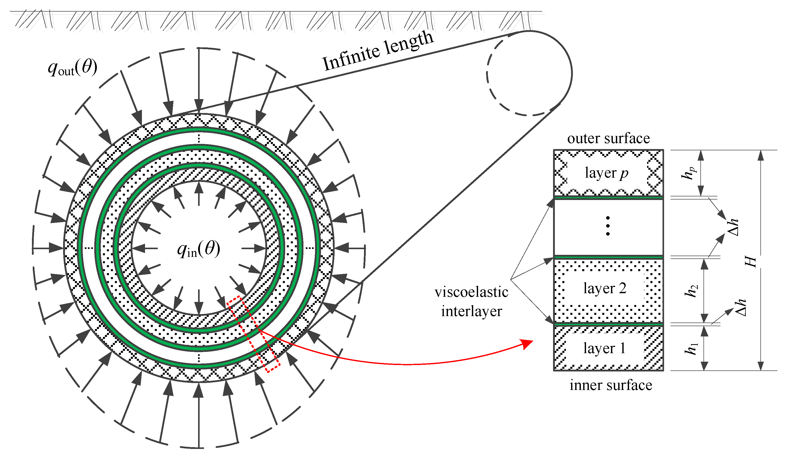
As shown in Figure 1, a composite pipe has an inner radius, $R_{in}$, an outer radius, $R_{out}$, and infinite length; it consists of p pipe layers with thickness $h_i$, bonded by interlayers with thickness $\Delta h$, in which i means the layer index (i = 1, 2, …, p).

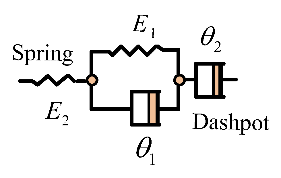
The pipe layers and the bonding interlayer both have viscoelastic properties, which are described by the Burgers model (Figure 2), with elastic moduli given as follows (Equation (1)):

$$E_i^{}(t)=E_1^i{\mathrm{e}}^{-t/{\theta }_1^i}+E_2^i{\mathrm{e}}^{-t/{\theta }_2^i},E_{}^{*}(t)=E_1^{*}{\mathrm{e}}^{-t/{\theta }_1^{*}}+E_2^{*}{\mathrm{e}}^{-t/{\theta }_2^{*}},$$

(1)

in which the symbol * denotes the variable belonging to the interlayer; $E_1^i$, $E_2^i$, $E_1^{*}$, and $E_2^{*}$ are the relaxation moduli, and ${\theta }_1^i$, ${\theta }_2^i$, ${\theta }_1^{*}$, and ${\theta }_2^{*}$ are the relaxation time. The pipe bears sustained compression with non-uniform pressure loads $q_{in}^{}(\theta )$ and $q_{out}^{}(\theta )$ acting on the inner and outer surfaces.

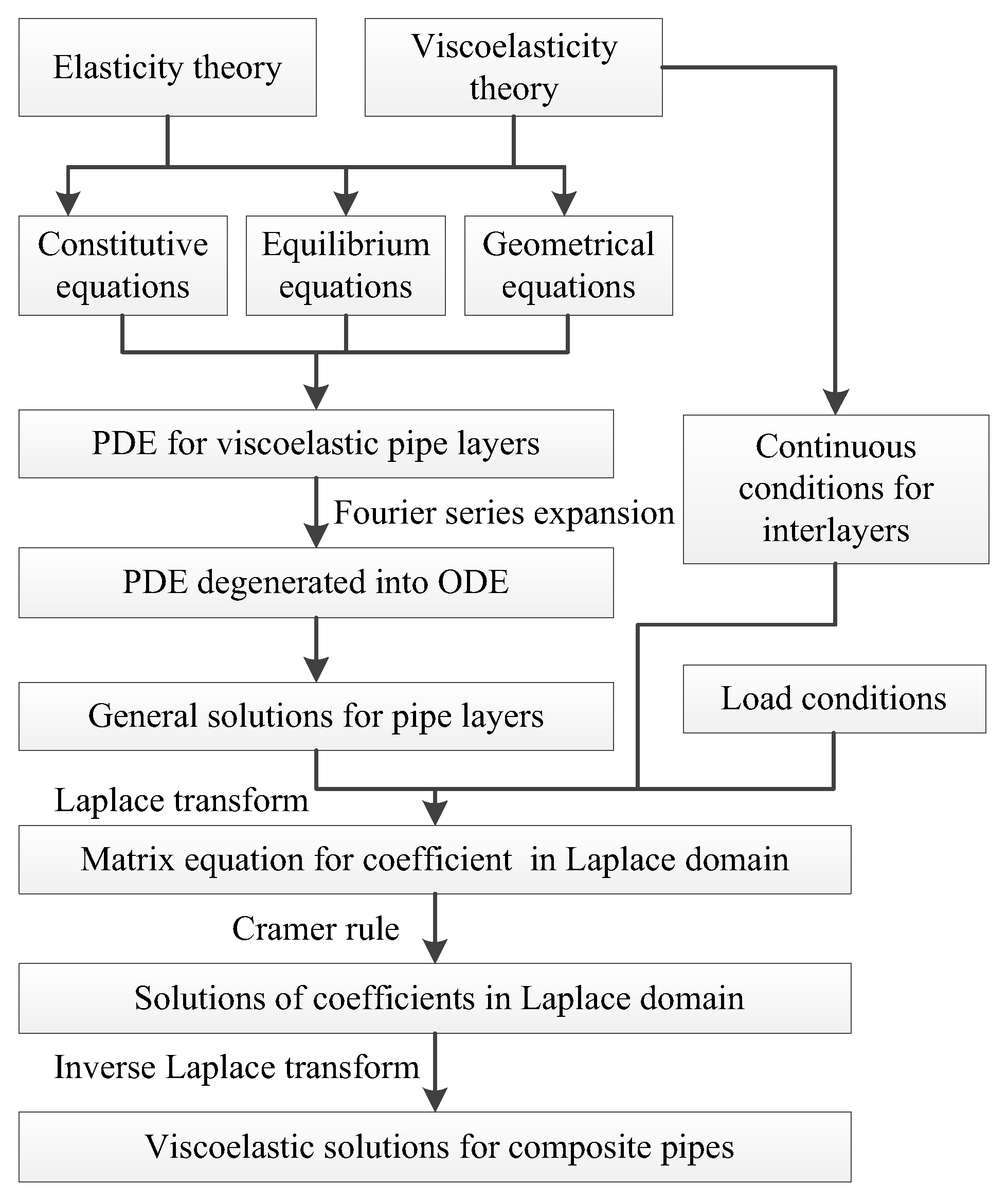
Figure 3 is the flow chart of the analytical process for the viscoelastic solutions of the composite pipes, which is described in detail in Section 2.1, Section 2.2 and Section 2.3.

2.1. General Solutions for the Viscoelastic Pipe Layers

The viscoelastic composite pipe, here with an infinite length, can be regarded as a two-dimensional plane-strain problem. On the basis of the elasticity theory combined with the viscoelasticity theory, the constitutive equations of i-th viscoelastic pipe layer are given in convolution form below (Equation (2)):

$${\sigma }_r^i(r,\theta ,t)=\frac{(1-{\mu }_i)}{(1+{\mu }_i)(1-2{\mu }_i)}{\displaystyle {\int }_{-\infty }^t\frac{d{E}_i(t-\xi )}{d(t-\xi )}}\left[\frac{\partial u_r^i(r,\theta ,\xi )}{\partial r}\right.+\frac{{\mu }_i}{1-{\mu }_i}\frac{u_r^i(r,\theta ,\xi )}{r}$$

$$+\frac{{\mu }_i}{1-{\mu }_i}\frac{1}{r}\left.\frac{\partial u_{\theta }^i(r,\theta ,\xi )}{\partial \theta }\right]d\xi ,$$

$${\sigma }_{\theta }^i(r,\theta ,t)=\frac{(1-{\mu }_i)}{(1+{\mu }_i)(1-2{\mu }_i)}{\displaystyle {\int }_{-\infty }^t\frac{d{E}_i(t-\xi )}{d(t-\xi )}}\left[\frac{{\mu }_i}{1-{\mu }_i}\frac{\partial u_r^i(r,\theta ,\xi )}{\partial r}\right.+\frac{u_r^i(r,\theta ,\xi )}{r}$$

$$+\frac{1}{r}\left.\frac{\partial u_{\theta }^i(r,\theta ,\xi )}{\partial \theta }\right]d\xi ,$$

$${\tau }_{r\theta }^i(r,\theta ,t)=\frac{1}{2(1+{\mu }_i)}{\displaystyle {\int }_{-\infty }^t\frac{d{E}_i(t-\xi )}{d(t-\xi )}}\left[\frac{1}{r}\frac{\partial u_r^i(r,\theta ,\xi )}{\partial \theta }\right.+\frac{\partial u_{\theta }^i(r,\theta ,\xi )}{\partial r}-\left.\frac{u_{\theta }^i(r,\theta ,\xi )}{r}\right]d\xi ,$$

(2)

in which ${\sigma }_r^i$, ${\sigma }_{\theta }^i$, and ${\tau }_{r\theta }^i$ represent the stress components; $u_r^i$ and $u_{\theta }^i$ are the displacement components; and ${\mu }_i$ is Poisson’s ratio. The stresses should satisfy the equilibrium relations, as depicted below (Equation (3)):

$$\frac{\partial {\sigma }_r^i}{\partial r}+\frac{1}{r}\frac{\partial {\tau }_{r\theta }^i}{\partial \theta }+\frac{{\sigma }_r^i-{\sigma }_{\theta }^i}{r}=0,\frac{1}{r}\frac{\partial {\sigma }_{\theta }^i}{\partial \theta }+\frac{\partial {\tau }_{r\theta }^i}{\partial r}+\frac{2{\tau }_{r\theta }^i}{r}=0.$$

(3)

The substitution of Equation (2) into Equation (3) and the elimination of stresses yield partial differential equations (PDE) involving integrals in regard to the displacement (Equation (4), as shown below):

$${\displaystyle {\int }_{-\infty }^t{E}_i^{}(t-\xi )}[\frac{1}{2}\frac{{\partial }^3{u}_{\theta }^i(r,\theta ,\xi )}{\partial r^2\partial \xi }+\frac{1}{2r}\frac{{\partial }^2{u}_{\theta }^i(r,\theta ,\xi )}{\partial r\partial \xi }-\frac{1}{2r^2}\frac{\partial u_{\theta }^i(r,\theta ,\xi )}{\partial \xi }+\frac{1}{2(1-2{\mu }_i)r}\frac{{\partial }^3{u}_r^i(r,\theta ,\xi )}{\partial r\partial \theta \partial \xi }$$

$$+\frac{3-4{\mu }_i}{2(1-2{\mu }_i)r^2}\frac{{\partial }^2{u}_r^i(r,\theta ,\xi )}{\partial \theta \partial \xi }+\frac{1-{\mu }_i}{(1-2{\mu }_i)r^2}\frac{{\partial }^3{u}_{\theta }^i(r,\theta ,\xi )}{\partial {\theta }^2\partial \xi }]d\xi =0,$$

$${\displaystyle {\int }_{-\infty }^t{E}_i^{}(t-\xi )}[\frac{1-{\mu }_i}{1-2{\mu }_i}\frac{{\partial }^3{u}_r^i(r,\theta ,\xi )}{\partial r^2\partial \xi }+\frac{1-{\mu }_i}{(1-2{\mu }_i)r}\frac{{\partial }^2{u}_r^i(r,\theta ,\xi )}{\partial r\partial \xi }-\frac{1-{\mu }_i}{(1-2{\mu }_i)r^2}\frac{\partial u_r^i(r,\theta ,\xi )}{\partial \xi }$$

$$+\frac{1}{2(1-2{\mu }_i)r}\frac{{\partial }^3{u}_{\theta }^i(r,\theta ,\xi )}{\partial r\partial \theta \partial \xi }-\frac{3-4{\mu }_i}{2(1-2{\mu }_i)r^2}\frac{{\partial }^2{u}_{\theta }^i(r,\theta ,\xi )}{\partial \theta \partial \xi }+\frac{1}{2r^2}\frac{{\partial }^3{u}_r^i(r,\theta ,\xi )}{\partial {\theta }^2\partial \xi }]d\xi =0.$$

(4)

To solve the above equations, the displacements, in terms of Fourier series, expanded, are used as follows (Equation (5)):

$$u_{\theta }^i(r,\theta ,t)={\Theta }_i^0(r,t)+{\displaystyle \sum _{m=1}^{\infty }{\Theta }_{im}^1(r,t)\sin (m\theta )}+{\displaystyle \sum _{m=1}^{\infty }{\Theta }_{im}^2(r,t)\cos (m\theta )},$$

$$u_r^i(r,\theta ,t)=R_i^0(r,t)+{\displaystyle \sum _{m=1}^{\infty }{R}_{im}^1(r,t)\cos (m\theta )}+{\displaystyle \sum _{m=1}^{\infty }{R}_{im}^2(r,t)\sin (m\theta )}.$$

(5)

For convenience, the above equations, each composed of three parts, are rearranged into two parts as shown below (Equation (6)):

$$u_{\theta }^i(r,\theta ,t)={\Theta }_i^0(r,t)+{\displaystyle \sum _{m=1}^{\infty }{\displaystyle \sum _{n=1}^2{\Theta }_{im}^n(r,t)[a_n\sin (m\theta )}}+b_n\cos (m\theta )],$$

$$u_r^i(r,\theta ,t)=R_i^0(r,t)+{\displaystyle \sum _{m=1}^{\infty }{\displaystyle \sum _{n=1}^2{R}_{im}^n(r,t)}[a_n\cos (m\theta )+b_n\sin (m\theta )]}.$$

(6)

in which $a_n=\frac{1-{(-1)}^n}{2}$, $b_n=\frac{1+{(-1)}^n}{2}$.

By substituting Equation (6) for Equation (4), Equation (4) is turned into ordinary differential equations (ODE) involving integrals and is decomposed as follows (Equation (7)):

$${\displaystyle {\int }_{-\infty }^t{E}_i^{}(t-\xi )}[\frac{{\partial }^3{\Theta }_i^0(r,\xi )}{\partial r^2\partial \xi }+\frac{1}{r}\frac{{\partial }^2{\Theta }_i^0(r,\xi )}{\partial r\partial \xi }-\frac{1}{r^2}\frac{\partial {\Theta }_i^0(r,\xi )}{\partial \xi }]d\xi =0,$$

$${\displaystyle {\int }_{-\infty }^t{E}_i^{}(t-\xi )}[\frac{{\partial }^3{R}_i^0(r,\xi )}{\partial r^2\partial \xi }+\frac{1}{r}\frac{{\partial }^2{R}_i^0(r,\xi )}{\partial r\partial \xi }-\frac{1}{r^2}\frac{\partial R_i^0(r,\xi )}{\partial \xi }]d\xi =0,$$

$${\displaystyle {\int }_{-\infty }^t{E}_i^{}(t-\xi )}[\frac{1-2{\mu }_i}{2}\frac{{\partial }^3{\Theta }_{im}^n(r,\xi )}{\partial r^2\partial \xi }+\frac{1-2{\mu }_i}{2}\frac{1}{r}\frac{{\partial }^2{\Theta }_{im}^n(r,\xi )}{\partial r\partial \xi }$$

$$-[(1-{\mu }_i)m^2+\frac{1-2{\mu }_i}{2}]\frac{1}{r^2}\frac{\partial {\Theta }_{im}^n(r,\xi )}{\partial \xi }+{(-1)}^{n+1}\frac{m}{2}\frac{1}{r}\frac{{\partial }^2{R}_{im}^{3-n}(r,\xi )}{\partial r\partial \xi }$$

$$+{(-1)}^{n+1}\frac{m(3-4{\mu }_i)}{2}\frac{1}{r^2}\frac{\partial R_{im}^{3-n}(r,\xi )}{\partial \xi }]d\xi =0,$$

$${\displaystyle {\int }_{-\infty }^t{E}_i^{}(t-\xi )}[\frac{1-2{\mu }_i}{2}\frac{{\partial }^3{R}_{im}^n(r,\xi )}{\partial r^2\partial \xi }+\frac{1-2{\mu }_i}{2}\frac{1}{r}\frac{{\partial }^2{R}_{im}^n(r,\xi )}{\partial r\partial \xi }$$

$$-[(1-{\mu }_i)m^2+\frac{1-2{\mu }_i}{2}]\frac{1}{r^2}\frac{\partial R_{im}^n(r,\xi )}{\partial \xi }+{(-1)}^{n+1}\frac{m}{2}\frac{1}{r}\frac{{\partial }^2{\Theta }_{im}^{3-n}(r,\xi )}{\partial r\partial \xi }$$

$$+{(-1)}^{n+1}\frac{m(3-4{\mu }_i)}{2}\frac{1}{r^2}\frac{\partial {\Theta }_{im}^{3-n}(r,\xi )}{\partial \xi }]d\xi =0,n=1,2.$$

(7)

The solutions of the above equations are as follows (Equation (8)):

$${\Theta }_i^0(r,t)=0,R_i^0(r,t)=r{A}_i^0(t)+r^{-1}{B}_i^0(t),$$

$${\Theta }_{im}^n(r,t)=r^{m+1}{A}_{im}^n(t)+r^{-m-1}{B}_{im}^n(t)+r^{m-1}{C}_{im}^n(t)+r^{-m+1}{D}_{im}^n(t),$$

$$R_{im}^n(r,t)={(-1)}^n\frac{m+4{\mu }_i-2}{m-4{\mu }_i+4}{r}^{m+1}{A}_{im}^n(t)+{(-1)}^{n+1}{r}^{-m-1}{B}_{im}^n(t)+{(-1)}^n{r}^{m-1}{C}_{im}^n(t)$$

$$+{(-1)}^{n+1}\frac{m-4{\mu }_i+2}{m+4{\mu }_i-4}{r}^{-m+1}{D}_{im}^n(t).$$

(8)

in which $A_i^0(t)$, $B_i^0(t)$, $A_{im}^n(t)$, $B_{im}^n(t)$, $C_{im}^n(t)$, and $D_{im}^n(t)$ are the undetermined coefficients. The substitution of Equation (8) into Equation (6) gives the general solutions (Equation (9)) for displacements of the i-th pipe layer as follows:

$$u_{\theta }^i(r,\theta ,t)={\displaystyle \sum _{n=1}^2{\displaystyle \sum _{m=1}^{\infty }[a_n\sin (m\theta )+b_n\cos (m\theta )][r^{m+1}{A}_{im}^n(t)+r^{-m-1}{B}_{im}^n(t)}}+r^{m-1}{C}_{im}^n(t)+r^{-m+1}{D}_{im}^n(t)],$$

$$u_r^i(r,\theta ,t)=r{A}_i^0(t)+r^{-1}{B}_i^0(t)+{\displaystyle \sum _{n=1}^2{\displaystyle \sum _{m=1}^{\infty }[a_n\cos (m\theta )+b_n\sin (m\theta )]}}[{(-1)}^n{\alpha }_{im}^1{r}^{m+1}{A}_{im}^n(t)$$

$$+{(-1)}^{n+1}{r}^{-m-1}{B}_{im}^n(t)+{(-1)}^n{r}^{m-1}{C}_{im}^n(t)+{(-1)}^{n+1}{\alpha }_{im}^2{r}^{-m+1}{D}_{im}^n(t)].$$

(9)

Then, by substituting Equation (9) for Equation (2), the general solutions for the stresses in the i-th pipe layer can be obtained as follows (Equation (10)):

$${\sigma }_r^i(r,\theta ,t)={\displaystyle {\int }_{-\infty }^t{E}_i(t-\xi )[}{\rho }_i^1\frac{\partial A_i^0(\xi )}{\partial \xi }-{\rho }_i^2{r}^{-2}\frac{\partial B_i^0(\xi )}{\partial \xi }]d\xi +{\displaystyle \sum _{n=1}^2{\displaystyle \sum _{m=1}^{\infty }[a_n\cos (m\theta )}}$$

$$+b_n\sin (m\theta )]{\displaystyle {\int }_{-\infty }^t{E}_i(t-\xi )}[{(-1)}^n{\beta }_{im}^1{r}^m\frac{\partial A_{im}^n(\xi )}{\partial \xi }+{(-1)}^n{\beta }_{im}^2{r}^{-m-2}\frac{\partial B_{im}^n(\xi )}{\partial \xi }$$

$$+{(-1)}^n{\beta }_{im}^3{r}^{m-2}\frac{\partial C_{im}^n(\xi )}{\partial \xi }+{(-1)}^n{\beta }_{im}^4{r}^{-m}\frac{\partial D_{im}^n(\xi )}{\partial \xi }]d\xi ,$$

$${\sigma }_{\theta }^i(r,\theta ,t)={\displaystyle {\int }_{-\infty }^t{E}_i(t-\xi )[}{\rho }_i^1\frac{\partial A_i^0(\xi )}{\partial \xi }+{\rho }_i^2{r}^{-2}\frac{\partial B_i^0(\xi )}{\partial \xi }]d\xi +{\displaystyle \sum _{n=1}^2{\displaystyle \sum _{m=1}^{\infty }[a_n\cos (m\theta )}}$$

$$+b_n\sin (m\theta )]{\displaystyle {\int }_{-\infty }^t{E}_i(t-\xi )}[{(-1)}^{n+1}{\chi }_{im}^1{r}^m\frac{\partial A_{im}^n(\xi )}{\partial \xi }+{(-1)}^{n+1}{\chi }_{im}^2{r}^{-m-2}\frac{\partial B_{im}^n(\xi )}{\partial \xi }$$

$$+{(-1)}^{n+1}{\chi }_{im}^3{r}^{m-2}\frac{\partial C_{im}^n(\xi )}{\partial \xi }+{(-1)}^{n+1}{\chi }_{im}^4{r}^{-m}\frac{\partial D_{im}^n(\xi )}{\partial \xi }]d\xi ,$$

$${\tau }_{r\theta }^i(r,\theta ,t)={\displaystyle \sum _{n=1}^2{\displaystyle \sum _{m=1}^{\infty }[a_n\sin (m\theta )+b_n\cos (m\theta )]{\displaystyle {\int }_{-\infty }^t{E}_i(t-\xi )}[{\zeta }_{im}^1{r}^m\frac{\partial A_{im}^n(\xi )}{\partial \xi }}}$$

$$-{\zeta }_{im}^2{r}^{-m-2}\frac{\partial B_{im}^n(\xi )}{\partial \xi }+{\zeta }_{im}^3{r}^{m-2}\frac{\partial C_{im}^n(\xi )}{\partial \xi }-{\zeta }_{im}^4{r}^{-m}\frac{\partial D_{im}^n(\xi )}{\partial \xi }]d\xi$$

(10)

in which

$${\alpha }_{im}^1=\frac{m+4{\mu }_i-2}{m-4{\mu }_i+4},{\alpha }_{im}^2=\frac{m-4{\mu }_i+2}{m+4{\mu }_i-4},{\rho }_i^1=\frac{1}{(1+{\mu }_i)(1-2{\mu }_i)},$$

$${\rho }_i^2=\frac{1}{1+{\mu }_i},{\beta }_{im}^1=\frac{(m+1)(m-2)}{(1+{\mu }_i)(m-4{\mu }_i+4)},{\beta }_{im}^2=\frac{(m+1)}{1+{\mu }_i},{\beta }_{im}^3=\frac{(m-1)}{1+{\mu }_i},$$

$${\beta }_{im}^4=\frac{(m-1)(m+2)}{(1+{\mu }_i)(m+4{\mu }_i-4)},{\chi }_{im}^1=\frac{(m+1)(m+2)}{(1+{\mu }_i)(m-4{\mu }_i+4)},{\chi }_{im}^2=\frac{(m+1)}{1+{\mu }_i},$$

$${\chi }_{im}^3=\frac{(m-1)}{1+{\mu }_i},{\chi }_{im}^4=\frac{(m-1)(m-2)}{(1+{\mu }_i)(m+4{\mu }_i-4)},{\zeta }_{im}^1=\frac{m(m+1)}{(1+{\mu }_i)(m-4{\mu }_i+4)},$$

$${\zeta }_{im}^2=\frac{(m+1)}{1+{\mu }_i},{\zeta }_{im}^3=\frac{(m-1)}{1+{\mu }_i},{\zeta }_{im}^4=\frac{m(m-1)}{(1+{\mu }_i)(m+4{\mu }_i-4)}.$$

2.2. Bonding Conditions

The interlayer slip effect is modeled here in this section. Here, only the shear deformation in the viscoelastic interlayer is considered, since the effect of ${\epsilon }_r^{*i}$ is negligible [39]. The constitutive equation involving the shear deformation for the i-th (i = 1, 2, …, p-1) viscoelastic interlayer is as follows (Equation (11)):

$${\tau }_{r\theta }^{*i}(\theta ,t)=\frac{1}{2(1+{\mu }_{}^{*})}{\displaystyle {\int }_{-\infty }^t{E}_{}^{*}(t-\xi )}\frac{\partial {\gamma }_{r\theta }^{*i}(\theta ,\xi )}{\partial \xi }d\xi .$$

(11)

The above equation is in the convolution form, which indicates the memory effect of viscoelasticity, i.e., that the stress at some point relies on the entire strain history. Since the interlayer thickness is far less than the thickness of the pipe layer, the displacement distribution through the radial direction in the interlayer can be assumed to be linear. Therefore, the geometrical relationship of the interlayers is given by (Equation (12)):

$$u_r^{i+1}(d_0^{i+1},\theta ,t)=u_r^i(d_1^i,\theta ,t),$$

$${\gamma }_{r\theta }^{*i}(\theta ,t)=\frac{u_{\theta }^{i+1}(d_0^{i+1},\theta ,t)-u_{\theta }^i(d_1^i,\theta ,t)}{\Delta h}+\frac{1}{d_1^i}\frac{\partial u_r^i(d_1^i,\theta ,t)}{\partial \theta }-\frac{u_{\theta }^i(d_1^i,\theta ,t)}{d_1^i},$$

(12)

in which $d_1^i$ and $d_0^i$ denote the r-coordinate values of the outer and inner surfaces of each pipe layer, respectively. The equilibrium relations for the neighboring pipe layers can be written as follows (Equation (13)):

$${\sigma }_r^{i+1}(d_0^{i+1},\theta ,t)={\sigma }_r^{*i}(\theta ,t)={\sigma }_r^i(d_1^i,\theta ,t),$$

$${\tau }_{r\theta }^{i+1}(d_0^{i+1},\theta ,t)={\tau }_{r\theta }^{*i}(\theta ,t)={\tau }_{r\theta }^i(d_1^i,\theta ,t).$$

(13)

By combining Equations (11)–(13), a relationship between the shear stress and the displacement components is obtained as follows (Equation (14)):

$${\tau }_{r\theta }^i(d_1^i,\theta ,t)=\frac{1}{2(1+{\mu }_{}^{*})\Delta h}{\displaystyle {\int }_{-\infty }^t{E}_{}^{*}(t-\xi )}[\frac{\partial u_{\theta }^{i+1}(d_0^{i+1},\theta ,\xi )}{\partial \xi }-\frac{\partial u_{\theta }^i(d_1^i,\theta ,\xi )}{\partial \xi }$$

$$+\frac{\Delta h}{d_1^i}\frac{{\partial }^2{u}_r^i(d_1^i,\theta ,\xi )}{\partial \theta \partial \xi }-\frac{\Delta h}{d_1^i}\frac{\partial u_{\theta }^i(d_1^i,\theta ,\xi )}{\partial \xi }]d\xi .$$

(14)

2.3. Determination of the Coefficients

The various loads which act on the surfaces of the pipe are described as follows (Equation (15)):

$${\sigma }_r^1=-q_{in}^{}(\theta ),{\tau }_{r\theta }^1=0,\mathrm{at}r=R_{in},$$

$${\sigma }_r^p=-q_{out}^{}(\theta ),{\tau }_{r\theta }^p=0,\mathrm{at}r=R_{out}.$$

(15)

In view of the general solutions, as given in series form, the loads $q_{in}(\theta )$ and $q_{out}(\theta )$ should also be expanded, as below (Equation (16)):

$$q_{in}^{}(\theta )=q_{in}^0+{\displaystyle \sum _{m=1}^{\infty }{q}_{in}^{m1}\cos (m\theta )}+{\displaystyle \sum _{m=2}^{\infty }{q}_{in}^{m2}\sin (m\theta )},$$

$$q_{out}^{}(\theta )=q_{out}^0+{\displaystyle \sum _{m=1}^{\infty }{q}_{out}^{m1}\cos (m\theta )}+{\displaystyle \sum _{m=2}^{\infty }{q}_{out}^{m2}\sin (m\theta )},$$

(16)

where

$$q_{in}^0=\frac{1}{2\pi }{\displaystyle {\int }_{-\pi }^{\pi }{q}_{in}^{}(\theta )}d\theta ,q_{out}^0=\frac{1}{2\pi }{\displaystyle {\int }_{-\pi }^{\pi }{q}_{out}^{}(\theta )}d\theta ,$$

$$q_{in}^{m1}=\frac{1}{\pi }{\displaystyle {\int }_{-\pi }^{\pi }{q}_{in}^{}(\theta )}\cos (m\theta )d\theta ,q_{out}^{m1}=\frac{1}{\pi }{\displaystyle {\int }_{-\pi }^{\pi }{q}_{out}^{}(\theta )}\cos (m\theta )d\theta ,$$

$$q_{in}^{m2}=\frac{1}{\pi }{\displaystyle {\int }_{-\pi }^{\pi }{q}_{in}^{}(\theta )}\sin (m\theta )d\theta ,q_{out}^{m2}=\frac{1}{\pi }{\displaystyle {\int }_{-\pi }^{\pi }{q}_{out}^{}(\theta )}\sin (m\theta )d\theta .$$

Equations (12)–(15) are then converted using the Laplace transform and expressed in matrix form, as shown below (Equations (17) and (18)):

$${\widehat{\Psi }}_0^i(s){\widehat{C}}_0^i(s)-{\widehat{\Phi }}_0^{i+1}(s){\widehat{C}}_0^{i+1}(s)=0,{\widehat{\Psi }}_{mn}^i(s){\widehat{C}}_{mn}^i(s)-{\widehat{\Phi }}_{mn}^{i+1}(s){\widehat{C}}_{mn}^{i+1}(s)=0,$$

(17)

$${\widehat{\Omega }}_0^{in}{\widehat{C}}_0^1(s)+{\widehat{\Omega }}_0^{out}{\widehat{C}}_0^p(s)=\frac{1}{s}{Q}_0^{},{\widehat{\Omega }}_{mn}^{in}{\widehat{C}}_{mn}^1(s)+{\widehat{\Omega }}_{mn}^{out}{\widehat{C}}_{mn}^p(s)=\frac{1}{s}{Q}_{mn}^{},$$

(18)

where

$${\widehat{C}}_0^i(s)={[\begin{array}{cc}{\widehat{A}}_i^0(s)& {\widehat{B}}_i^0(s)\end{array}]}^T,{\widehat{C}}_{mn}^i(s)={[\begin{array}{cccc}{\widehat{A}}_{im}^n(s)& {\widehat{B}}_{im}^n(s)& {\widehat{C}}_{im}^n(s)& {\widehat{D}}_{im}^n(s)\end{array}]}^T,$$

$$Q_0^{}={[\begin{array}{cc}{q}_{in}^0& q_{out}^0\end{array}]}^T,Q_{mn}^{}={[\begin{array}{cccc}{q}_{in}^{mn}& 0& q_{out}^{mn}& 0\end{array}]}^T,$$

and the over arcs mean that the variables are in the Laplace domain, such as ${\widehat{C}}_0^i(s)$; the details of the elements ${\widehat{\Psi }}_0^i(s)$, ${\widehat{\Phi }}_0^i(s)$, ${\widehat{\Psi }}_{mn}^i(s)$ and ${\widehat{\Phi }}_{mn}^i(s)$ can be found in Appendix A Equation (A1); the details of ${\widehat{\Omega }}_0^{in}$, ${\widehat{\Omega }}_0^{out}$, ${\widehat{\Omega }}_{mn}^{in}$ and ${\widehat{\Omega }}_{mn}^{out}$ can be found in Appendix A Equation (A2). The combination of Equations (17) and (18) yields the following (Equation (19)) matrix equation for the undetermined coefficients in the Laplace domain:

$${\widehat{M}}_0^{}(s){\widehat{X}}_0^{}(s)=\frac{1}{s}{A}_0^{},{\widehat{M}}_{mn}^{}(s){\widehat{X}}_{mn}^{}(s)=\frac{1}{s}{A}_{mn}^{},$$

(19)

where

$${\widehat{X}}_0^{}(s)=\left[\begin{array}{c}{\widehat{C}}_0^1(s)\\ {\widehat{C}}_0^2(s)\\ \cdot \cdot \cdot \\ {\widehat{C}}_0^p(s)\end{array}\right],{\widehat{X}}_{mn}^{}(s)=\left[\begin{array}{c}{\widehat{C}}_{mn}^1(s)\\ {\widehat{C}}_{mn}^2(s)\\ \cdot \cdot \cdot \\ {\widehat{C}}_{mn}^p(s)\end{array}\right],A_0^{}=\left[\begin{array}{c}0\\ \cdot \cdot \cdot \\ 0\\ Q_0^{}\end{array}\right],A_{mn}^{}=\left[\begin{array}{c}0\\ \cdot \cdot \cdot \\ 0\\ Q_{mn}^{}\end{array}\right],$$

$${\widehat{M}}_0^{}(s)=\left[\begin{array}{ccccc}{\widehat{\Psi }}_0^1(s)& -{\ddot{\Phi }}_0^2(s)& 0& \cdot \cdot \cdot & \cdot \cdot \cdot \\ 0& {\widehat{\Psi }}_0^2(s)& -{\widehat{\Phi }}_0^3(s)& 0& \cdot \cdot \cdot \\ & & \cdot \cdot \cdot & \cdot \cdot \cdot & \\ \cdot \cdot \cdot & 0& {\widehat{\Psi }}_0^i(s)& -{\widehat{\Phi }}_0^{i+1}(s)& 0\\ & & \cdot \cdot \cdot & \cdot \cdot \cdot & \\ \cdot \cdot \cdot & \cdot \cdot \cdot & 0& {\widehat{\Psi }}_0^{p-1}(s)& -{\widehat{\Phi }}_0^p(s)\\ {\widehat{\Omega }}_0^{in}& 0& \cdot \cdot \cdot & 0& {\widehat{\Omega }}_0^{out}\end{array}\right],$$

$${\widehat{M}}_{mn}^{}(s)=\left[\begin{array}{ccccc}{\widehat{\Psi }}_{mn}^1(s)& -{\widehat{\Phi }}_{mn}^2(s)& 0& \cdot \cdot \cdot & \cdot \cdot \cdot \\ 0& {\widehat{\Psi }}_{mn}^2(s)& -{\widehat{\Phi }}_{mn}^3(s)& 0& \cdot \cdot \cdot \\ & & \cdot \cdot \cdot & \cdot \cdot \cdot & \\ \cdot \cdot \cdot & 0& {\widehat{\Psi }}_{mn}^i(s)& -{\widehat{\Phi }}_{mn}^{i+1}(s)& 0\\ & & \cdot \cdot \cdot & \cdot \cdot \cdot & \\ \cdot \cdot \cdot & \cdot \cdot \cdot & 0& {\widehat{\Psi }}_{mn}^{p-1}(s)& -{\widehat{\Phi }}_{mn}^p(s)\\ {\widehat{\Omega }}_{mn}^{in}& 0& \cdot \cdot \cdot & 0& {\widehat{\Omega }}_{mn}^{out}\end{array}\right].$$

By using the Cramer rule and fraction expansion, the coefficients are further expressed as follows (Equation (20)):

$${\widehat{X}}_0^j(s)=\frac{\left|{\widehat{M}}_0^j(s)\right|}{s\left|{\widehat{M}}_0^{}(s)\right|}=\frac{{\displaystyle \sum _{\lambda =0}^{p-1}{\omega }_0^{j\lambda }{s}^{\lambda }}}{{\displaystyle \sum _{\lambda =0}^{p-1}{\eta }_0^{\lambda }{s}^{\lambda +1}}}={\displaystyle \sum _{\alpha =1}^p\frac{c_0^{\alpha }}{s-s_0^{\alpha }}},$$

$${\widehat{X}}_{mn}^k(s)=\frac{\left|{\widehat{M}}_{mn}^k(s)\right|}{s\left|{\widehat{M}}_{mn}^{}(s)\right|}=\frac{{\displaystyle \sum _{\lambda =0}^{2p-2}{\omega }_{mn}^{k\lambda }{s}^{\lambda }}}{{\displaystyle \sum _{\lambda =0}^{2p-2}{\eta }_{mn}^{\lambda }{s}^{\lambda +1}}}={\displaystyle \sum _{\beta =1}^{2p-1}\frac{c_{mn}^{\beta }}{s-s_{mn}^{\beta }}},j=1,2,\dots ,2p,k=1,2,\dots ,4p,$$

(20)

where

$${\omega }_0^{j\lambda }=\underset{s\to +\infty }{\lim }\frac{1}{s^{\lambda }}\left(\left|M_0^j(s)\right|-{\displaystyle \sum _{a=\lambda +1}^{p-1}{\omega }_0^{ja}{s}^a}\right),{\eta }_0^{\lambda }=\underset{s\to +\infty }{\lim }\frac{1}{s^{\lambda }}\left(\left|M_0^{}(s)\right|-{\displaystyle \sum _{a=\lambda +1}^{p-1}{\eta }_0^a{s}^a}\right),$$

$${\omega }_{mn}^{k\lambda }=\underset{s\to +\infty }{\lim }\frac{1}{s^{\lambda }}\left(\left|M_{mn}^k(s)\right|-{\displaystyle \sum _{a=\lambda +1}^{2p-2}{\omega }_{mn}^{ka}{s}^a}\right),{\eta }_{mn}^{\lambda }=\underset{s\to +\infty }{\lim }\frac{1}{s^{\lambda }}\left(\left|M_{mn}^{}(s)\right|-{\displaystyle \sum _{a=\lambda +1}^{2p-2}{\eta }_{mn}^a{s}^a}\right),$$

$$c_{\alpha 0}^j=\frac{{\displaystyle \sum _{\lambda =0}^{p-1}{\omega }_0^{j\lambda }{(s_0^{\alpha })}^{\lambda }}}{{\displaystyle \sum _{\lambda =0}^{p-1}(\lambda +1){\eta }_0^{\lambda }{(s_0^{\alpha })}^{\lambda }}},c_{\beta mn}^k=\frac{{\displaystyle \sum _{\lambda =0}^{2p-2}{\omega }_{mn}^{k\lambda }{(s_0^{\beta })}^{\lambda }}}{{\displaystyle \sum _{\lambda =0}^{2p-2}(\lambda +1){\eta }_{mn}^{\lambda }{(s_0^{\beta })}^{\lambda }}},$$

and $s_0^{\alpha }$ and $s_{mn}^{\beta }$ are roots of ${\displaystyle \sum _{\lambda =0}^{p-1}{\eta }_0^{\lambda }{s}^{\lambda +1}}=0$ and ${\displaystyle \sum _{\lambda =0}^{2p-2}{\eta }_{mn}^{\lambda }{s}^{\lambda +1}}=0$, respectively. Taking the inverse Laplace transform of Equation (20), the coefficients of the time domain can be obtained as follows (Equation (21)):

$$X_0^j(t)={\displaystyle \sum _{\alpha =1}^p{c}_{\alpha 0}^j{e}^{-s_0^{\alpha }t}},X_{mn}^k(t)={\displaystyle \sum _{\beta =1}^{2p-1}{c}_{\beta mn}^k{e}^{-s_{mn}^{\beta }t}},$$

(21)

Finally, the analytical solutions for the viscoelastic composite pipe are determined via substitution of the coefficients of the time domain into Equation (10).

3. Results and Discussion

In the following, for the purpose of investigating the compressive creep of the viscoelastic composite pipe, several analyses of viscoelastic sandwich pipes are carried out, with parameters fixed at $q_{in}(\theta )$ = 0.2 N/mm², R_in = 600 mm, h₁ = h₃ = 20 mm, h₂ = 60 mm, $\Delta h$ = 0.5 mm, and ${\mu }_i$ = ${\mu }_{}^{*}$ = 0.3, unless otherwise stated.

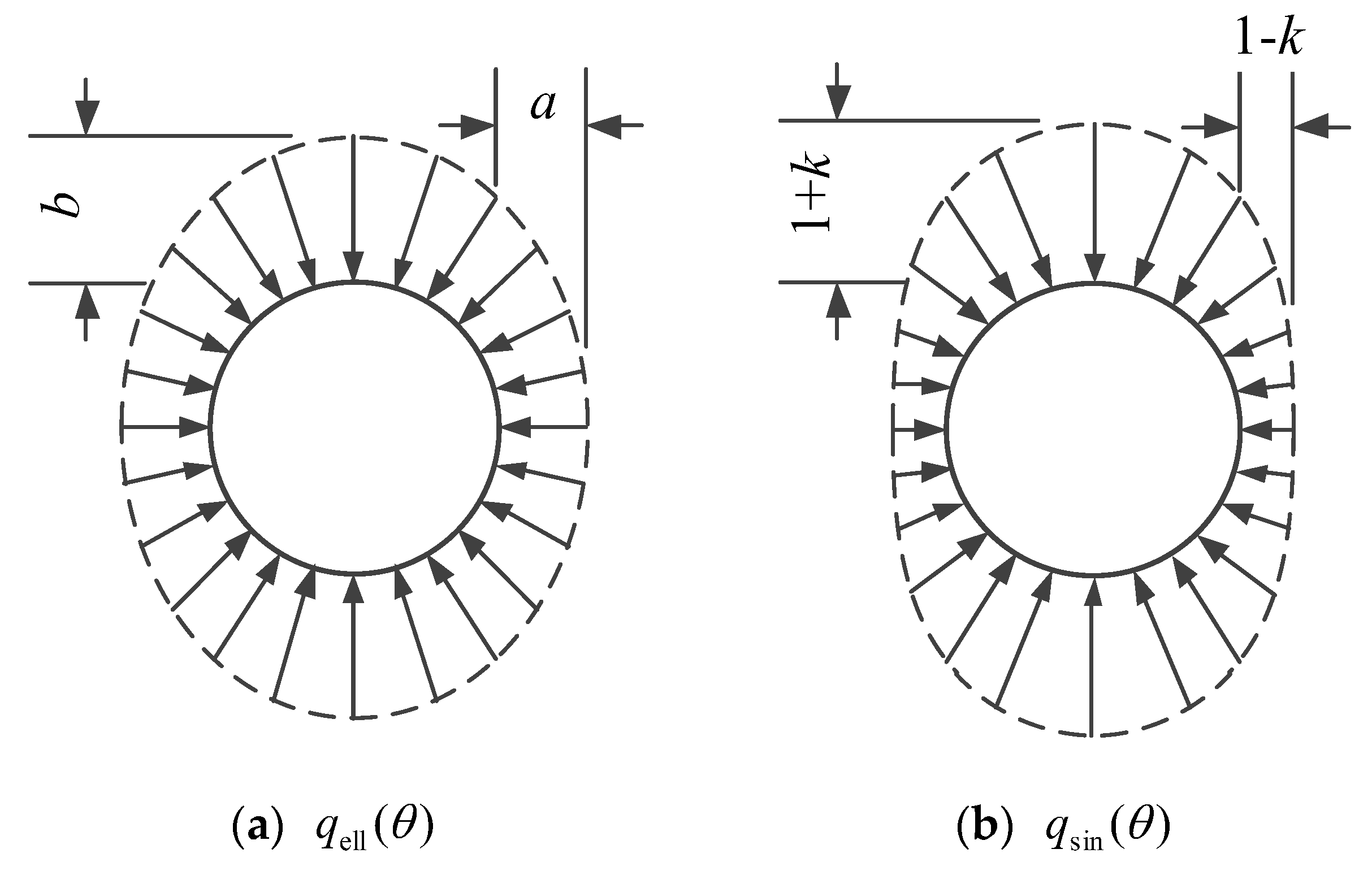
As shown in Figure 4, the two non-uniform load functions are defined beforehand, including the elliptic load $q_{\mathrm{ell}}(\theta )$ and the sinusoidal load $q_{\sin }(\theta )$, which are expressed as follows (Equation (22)):

$$q_{\mathrm{ell}}(\theta )=\frac{gb}{2\sqrt{g^2{\cos }^2(\theta )+{\sin }^2(\theta )}},q_{\sin }(\theta )=0.5+0.5k\sin (2\theta -\frac{\pi }{2}),$$

(22)

where $g=b/a$; a and b are the lengths of minor axis and major axis in the ellipse, respectively; and k is the non-uniformity degree for the sinusoidal load. Some variables are defined as follows (Equation (23)):

$${\sigma }_f^{}={\sigma }_{\theta }^1\mathrm{at}\theta =0.5\pi ,r=d_0^1;{\tau }_{}^{*}={\tau }_{r\theta }^1\mathrm{at}\theta =0.25\pi ,r=d_1^1;$$

$${\tau }_c^{}={\tau }_{r\theta }^2\mathrm{at}\theta =0.25\pi ,r=0.5(d_0^2+d_1^2);u_r^f=u_r^1\mathrm{at}\theta =0.5\pi ,r=d_0^1,$$

(23)

in which a variable with superscripts f or c respectively attaches to the facial (i = 1, 3) or core (i = 2) layer. Additionally, the symbol $\left|\right|$ means the absolute value and the subscript max represent the maximum value.

3.1. Convergence and Comparison Verifications

The first step is to verify the convergence property of the present solution. Here, the viscoelastic sandwich pipe with interlayers is under $q_{out}^{}(\theta )$ = $q_{\mathrm{ell}}(\theta )$ with g = 2, in which all layers follow a proportion relation with $E_c(t)$ = $E_f(t)$/3 = 10⁴ $E_i^{*}(t)$, and the viscoelastic parameters of the core layer are set as $E_1^c$ = 1125.11 MPa, $E_2^c$ = 2144.89 MPa, ${\theta }_1^c$ = 2.519 × 10⁷ s, and ${\theta }_2^c$ = 2.097 × 10⁵ s [40]. The results of the stresses and displacements with different series terms, N, which are truncated from the infinite series in the present solutions, are listed in

Table 1. The stresses and displacements of the solution here with different series terms.

N	${\mathit{\sigma }}_{\mathit{\theta }}^1$ [MPa]	${\mathit{\sigma }}_{\mathit{r}}^1$ [MPa]	${\mathit{\tau }}_{\mathit{r}\mathit{\theta }}^1$ [MPa]	${\mathit{u}}_{\mathit{r}}^1$ [mm]	${\mathit{u}}_{\mathit{\theta }}^1$ [mm]
2	−42.94	0.1024	−0.3672	−83.24	−25.37
4	−43.97	0.1022	−0.4251	−83.60	−25.54
6	−43.56	0.1046	−0.4289	−83.54	−25.54
8	−43.45	0.1059	−0.4288	−83.54	−25.54
10	−43.45	0.1059	−0.4287	−83.54	−25.54

Note: The stresses and displacements are at t = 10⁵ s and located at θ = $\pi /3$, r = 620 mm in pipe layer 1.

. Table 1 shows the rapid convergence of the present results, which reach an accuracy of four significant digits when N = 10. Hence, from here onward, the number of series term will be fixed at N = 10.

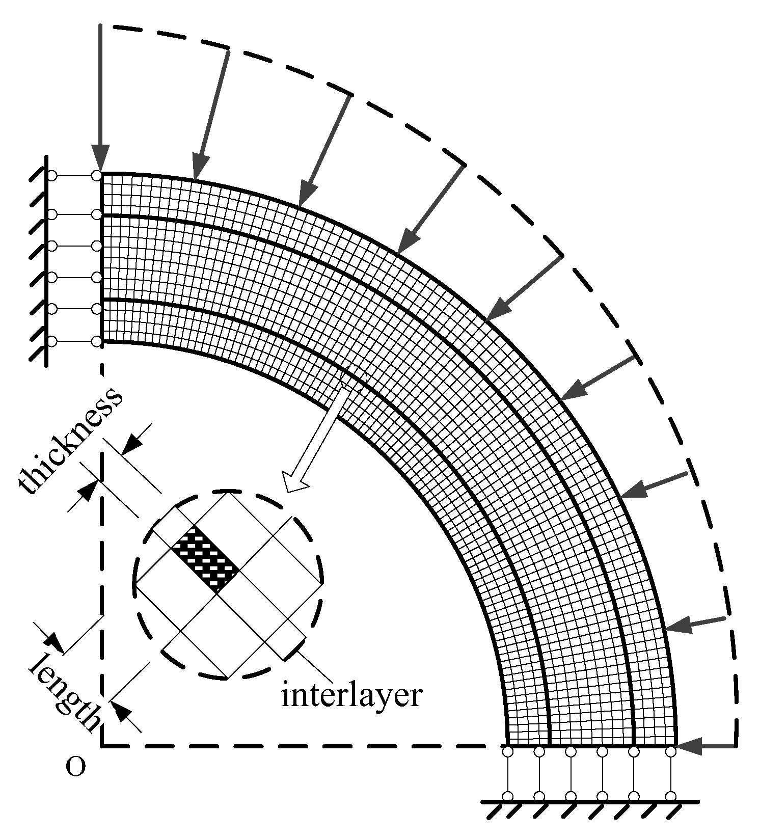
Additionally, the present solution is compared with the FE solution from ANSYS, in which the PLANE-183 element is taken to simulate the viscoelastic pipe layers and interlayers. Figure 5 shows the schematic diagram of the FE model, which only considers ¼ of the pipe due to the symmetry of the structure. The interlayer, facial layer, and core layer of the pipe are divided into 1, ζ and 2ζ equal parts in the r direction, respectively; all layers are evenly divided into 8ζ parts in the θ direction. The results of the comparison between the present solution and the FE solution with different ζ when t = 10⁵ s are shown in

Table 2. The results of comparison between the present solution and the FE solution.

FE results with Different ζ							Present
ζ	2	4	6	10	20	30	Solution
${\sigma }_{\theta }^1$ [MPa]	−54.62	−48.27	−45.51	−44.37	−43.98	−43.86	−43.45
Error (%)	25.7	11.1	4.74	2.11	1.23	0.941	/
${\tau }_{r\theta }^1$ [MPa]	−0.4689	−0.4420	−0.4399	−0.4368	−0.4336	−0.4328	−0.4287
Error (%)	9.37	3.11	2.63	1.89	1.15	0.956	/
$u_r^1$ [mm]	−84.28	−84.16	−84.08	−84.03	−84.02	−83.99	−83.54
Error (%)	0.886	0.737	0.651	0.583	0.569	0.534	/

. It can be seen from Table 2 that the FE solution tends to approach the present solution as the density of the mesh increases. ${\sigma }_{\theta }^1$, ${\tau }_{r\theta }^1$ and $u_r^1$ have errors of 0.941%, 0.956%, and 0.534%, respectively, when ζ = 30. That is to say, the results of the FE solutions can become more precise when the FE mesh is more refined. It is worth noting that this model takes more time and has a high cost in terms of computation due to the fine mesh and the time step division. The present analytical model is advantageous in its computational efficiency compared with the FE method. The reason for this is that the FE model calculates results from the beginning to a certain time gradually by using the viscoelastic material in question, while the present analytical model has the ability to calculate the results at any time directly.

The present solution can be degenerated into the solution for a laminated arch by keeping one part of the expansion term from the Fourier series for displacements in Equation (5) and replacing m with $m\pi /\beta$, as follow (Equation (24)):

$$u_{\theta }^i(r,\theta ,t)={\displaystyle \sum _{m=1}^{\infty }{\Theta }_{im}^2(r,t)\cos (m\pi \theta /\beta )},$$

$$u_r^i(r,\theta ,t)={\displaystyle \sum _{m=1}^{\infty }{R}_{im}^2(r,t)\sin (m\pi \theta /\beta )}.$$

(24)

in which $\beta$ is the angle of the laminated arch. A comparison between the present solution and the EB solution from Galuppi and Royer-Carfagni [41] is made. In the EB solution, the interlayers are regarded as viscoelastic material and are simulated by a generalized Maxwell model, with a time-dependent modulus written in Prony series form, expressed as follows:

$$G^{*}(t)=G_{\infty }^{*}+{\displaystyle \sum _{j=1}^M{G}_j^{*}{e}^{-t/{\theta }_{G,j}}}.$$

(25)

The arches are considered to be composed of 2 elastic layers with a viscoelastic interlayer, which is subjected to the uniform radial load $q(\theta )$ = 7.5 × 10⁻⁴ N/mm². S and $R_m$, calculated by S = $\beta R_m$ and $R_m$ = $R_{in}$ + 0.5 H, mean the average arch length and radius, respectively. The parameters of the arch are defined as $E_1$ = $E_2$ = 70 GPa, ${\mu }_1$ = ${\mu }_2$ = ${\mu }^{*}$ = 0.3, $\beta$ = 0.25π, h₁ = h₂, S = 4000 mm, Δh = 0.5 mm. The viscoelastic parameters of the interlayer are taken from the research by Wu et al. [42].

Table 3. Comparisons of the mid-span deflection among the present and EB solution when t = 10¹⁰ s at different ratios S/H.

S/H	100	50	30	20	15	10
Present [mm]	−30.61	−3.863	−0.8480	−0.2560	−0.1099	−0.03373
EB [mm]	−30.49	−3.811	−0.8232	−0.2439	−0.1029	−0.03049
Error of EB (%)	0.392	1.35	2.92	4.73	6.37	9.61

reveals the comparison results for the mid-span deflection, i.e., $u_r^i$ at θ = 0.5β, r = $R_m$, when t = 10¹⁰ s at different arch length-thickness ratios S/H. In Table 3, the mid-span deflection based on the present solution and the EB solution has a high consistency for a large S/H. Nevertheless, as S/H diminishes, the error of the results becomes larger, and the results have a maximum error of 9.61% at S/H = 10.

3.2. Effect of Material Configuration

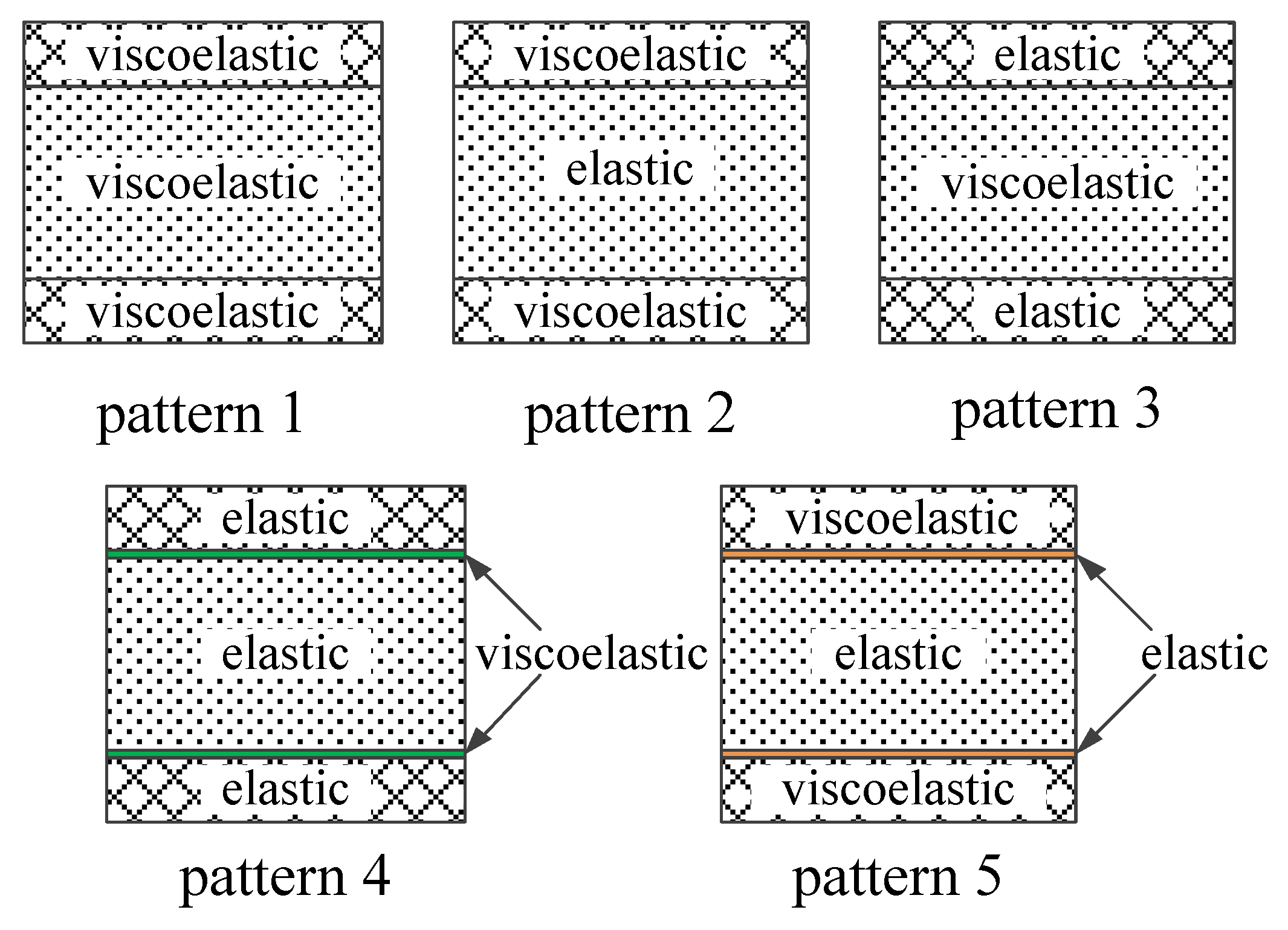
The effect of the material configuration is investigated in this section. Here, the pipe is under the sinusoidal load $q_{\sin }(\theta )$ with k = 0.4. Five patterns of material configuration are analyzed, as shown in Figure 6.

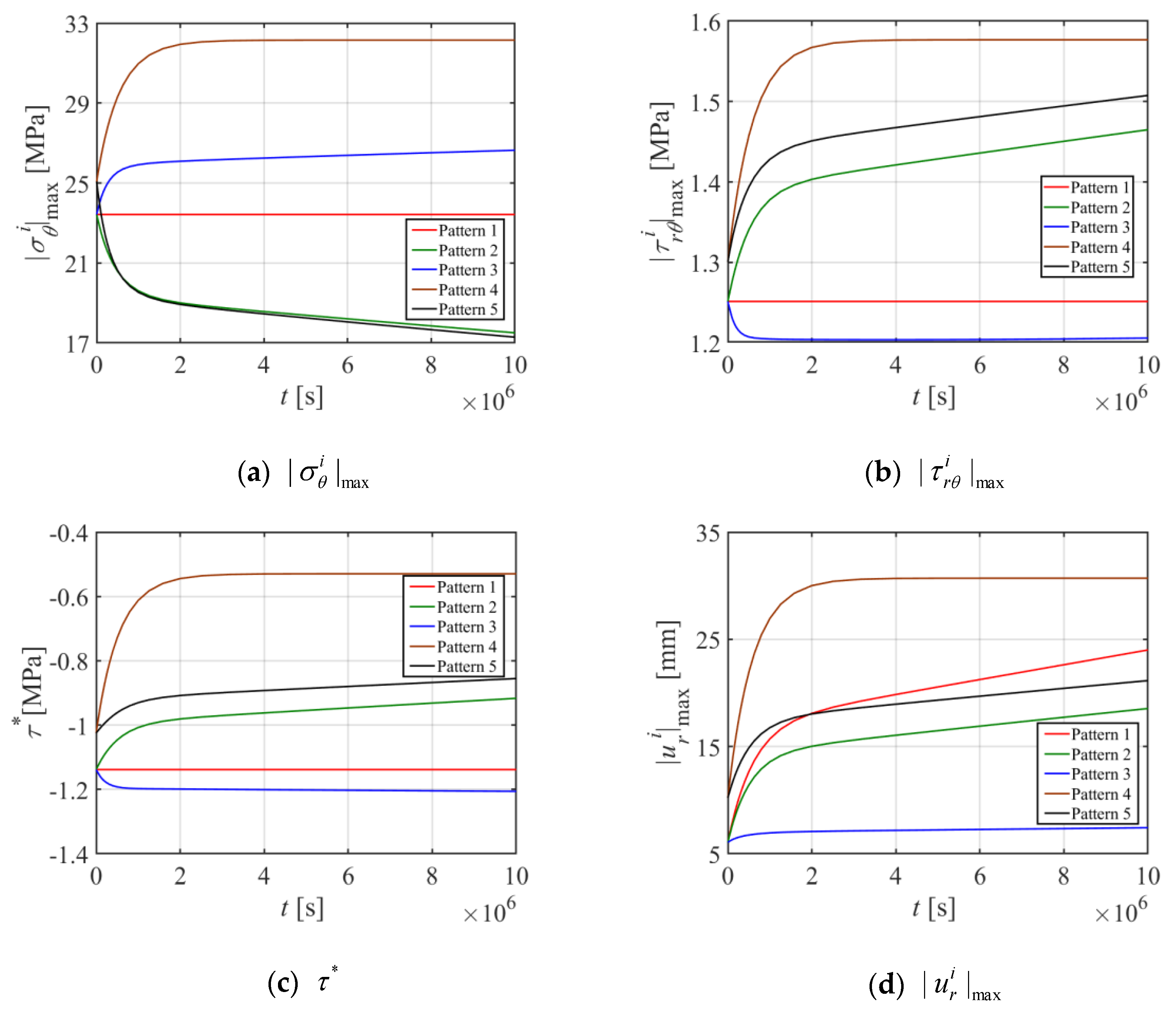
The moduli of the viscoelastic layers are the same as those in Section 3.1, while the modulus for the elastic layer is taken as the initial value of the viscoelastic case, i.e., $E_c^{}$ = $E_c^{}(0)$ or $E_f^{}$ = $E_f^{}(0)$. The interlayer in pattern 4 has the standard linear solid model [43], with viscoelastic parameters taken as $G_1^{*}$ = 1 MPa, $G_{\infty }^{*}$ = 0.1 MPa, and ${\theta }_{G,1}^{*}$ = 1 × 10⁵ s. The interlayer in the pattern 5 exhibits elasticity, in which $G^{*}$ = 1.1 MPa. Figure 7 shows the changes in the stresses and displacements with time in the five patterns.

From Figure 7, it is found that, in pattern 1, $|{\sigma }_{\theta }^i{|}_{\max }$, $|{\tau }_{r\theta }^i{|}_{\max }$ and ${\tau }_{}^{*}$ always remain constant with time, which is like the behavior of a purely elastic material. A reason can be given to elucidate this phenomenon. Although the pipe is made up of viscoelastic materials, the bending moment of any cross-section in the pipe remains unchanged as time goes on. Furthermore, based on the findings of the studies of laminated structures [44,45], the proportion of the modulus between neighboring layers determines the stress distribution with a constant cross-section bending moment, but the deformation is dependent on the absolute value of the modulus. In pattern 2, $|{\sigma }_{\theta }^i{|}_{\max }$ decreases with t but $|{\tau }_{r\theta }^i{|}_{\max }$ and ${\tau }_{}^{*}$ increases with t. This is because the moduli of the viscoelastic facial layers degenerate with t, and $|{\sigma }_{\theta }^i{|}_{\max }$ and $|{\tau }_{r\theta }^i{|}_{\max }$ occur in the facial and core layers, respectively. Compared with pattern 5, when the elastic interlayer is exited, $|{\sigma }_{\theta }^i{|}_{\max }$ shows little change, while the values of $|{\tau }_{r\theta }^i{|}_{\max }$, ${\tau }_{}^{*}$ and $|u_r^i{|}_{\max }$ decrease. The change rules for the stresses in pattern 3 are exactly in contrast to those of pattern 2. The values of $|u_r^i{|}_{\max }$ in patterns 1–3 and 5 all increase with t, and the rates of increase gradually tend to become constant. In pattern 4, $|{\sigma }_{\theta }^i{|}_{\max }$, $|{\tau }_{r\theta }^i{|}_{\max }$, ${\tau }_{}^{*}$ and $|u_r^i{|}_{\max }$ all increase with time, the values are always constant, and the long-term values that represent the adjacent layers in the pipe are almost not bonded. This study can be referenced for the design of composite pipes taking into account their long-term performance.

3.3. Effect of Load Uniformity Degree

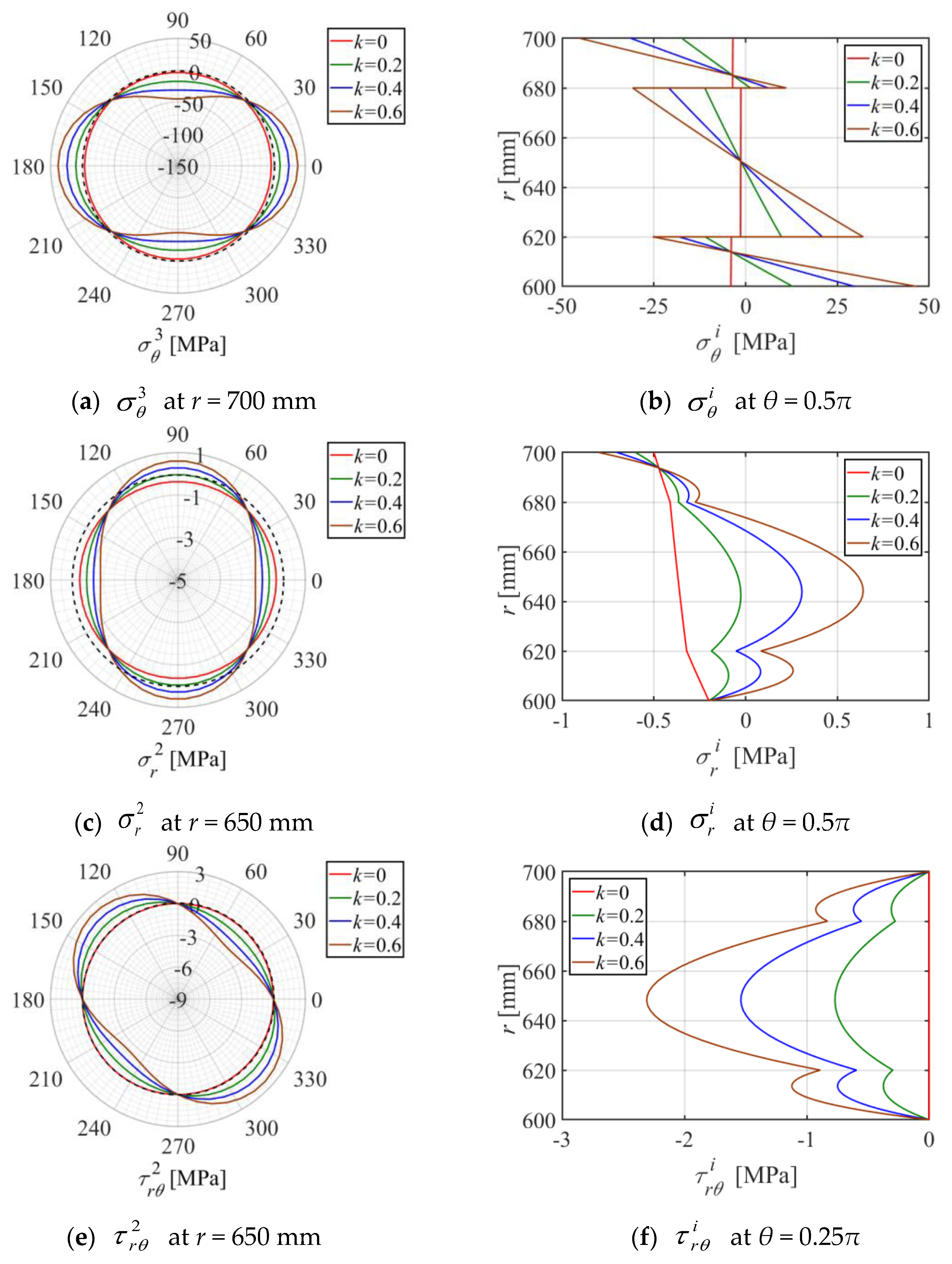
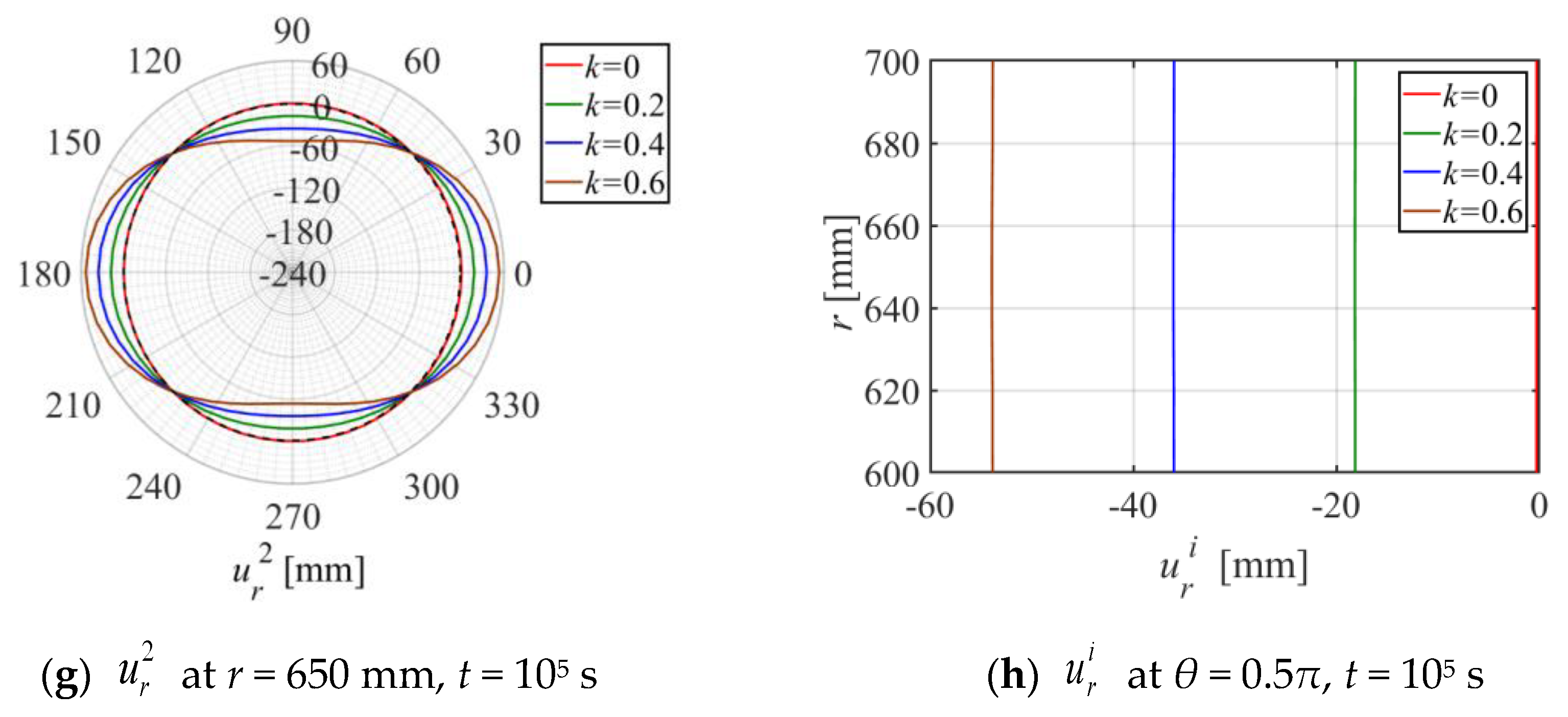
Here, the effects of the degree of load uniformity on the stress and displacement distribution are explored. For this, the pipe is under the sinusoidal load, $q_{\sin }(\theta )$, and k is variable. The special case k = 0 means that the load is uniform, and the degree of load uniformity increases with k. The moduli in the layers have the same value as those in Section 3.1. The r-direction distribution of stresses and displacements through the circumferential direction are shown in Figure 8.

As shown in Figure 8, for the uniform case of k = 0, ${\sigma }_{\theta }^i$, ${\sigma }_r^i$, ${\tau }_{r\theta }^i$, and $u_r^i$ have very small values, while these values increase remarkably as k increases. Along the circumference of the pipe, the changes in stresses and displacements follow the shapes of trigonometric functions, and the location of each maximum has a difference of π/2 from the location of its respective minimum. The maxima of ${\sigma }_{\theta }^i$, ${\sigma }_r^i$, ${\tau }_{r\theta }^i$, and $u_r^i$ happen at θ = 0, π/2, 3π/4, and 0, respectively. Through the thickness direction of the pipe, ${\sigma }_{\theta }^i$ shows a zig-zag distribution, ${\sigma }_r^i$ and ${\tau }_{r\theta }^i$ exhibit multi-peak distributions, and $u_r^i$ stays constant. In practical engineering, for composite pipes under long duration loads, the effect of the degree of load uniformity cannot be ignored, and a reasonable structure design is necessary for composite pipes under different environmental conditions.

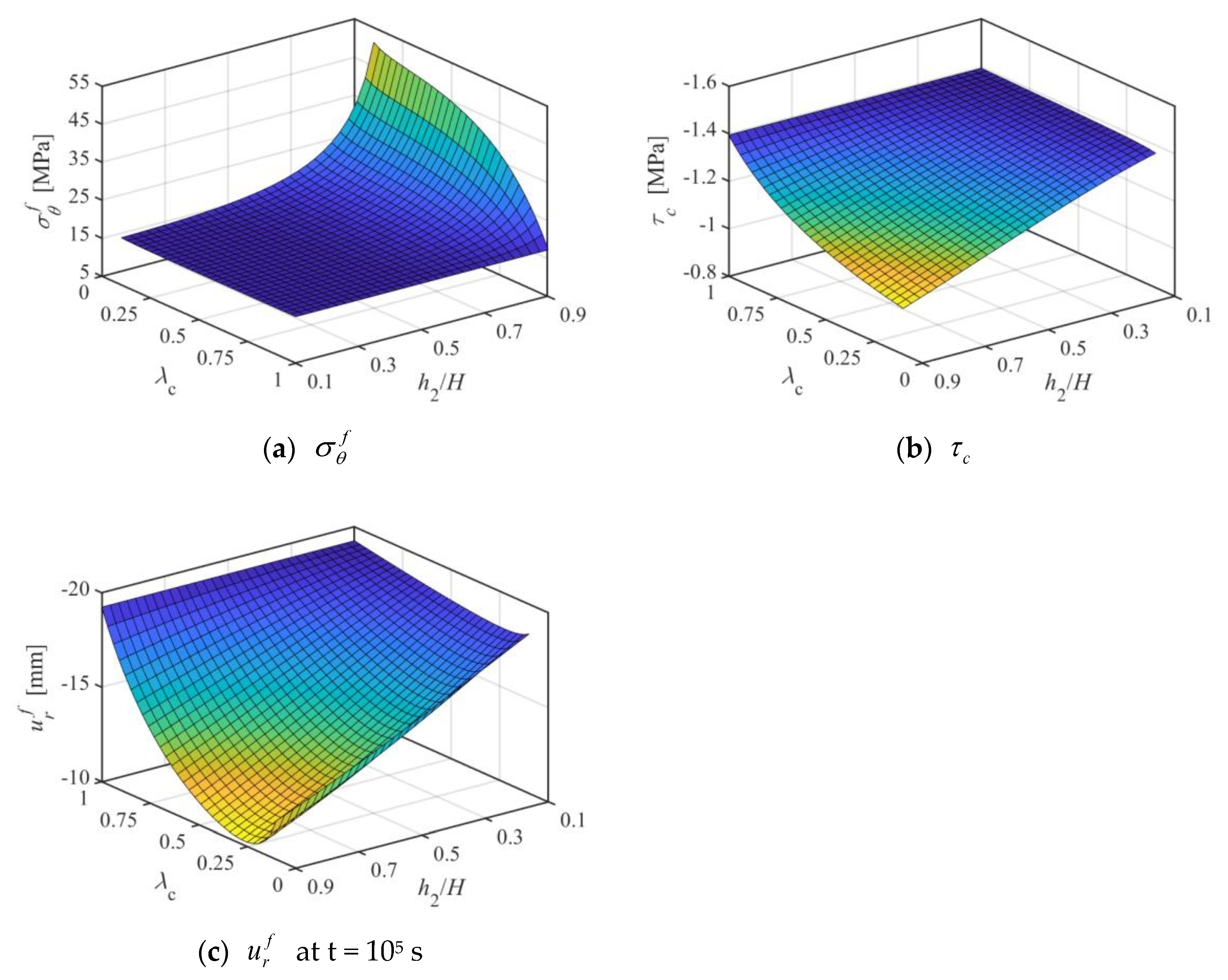
3.4. Optimization of Stresses and Displacements

When the pipe is under the sinusoidal load $q_{\sin }(\theta )$ with k = 0.4, h₁ = h₃ and E₁(t) = E₃(t), in which the moduli of all viscoelastic layers remain proportional. Here, an optimization of the stresses and displacements in the pipes achieved by adjusting the modulus and the thickness of each layer is presented in Figure 9. The optimization is based on the premise that the average modulus, $\overline{E}(t)$, calculated by ${\displaystyle \sum E_i(t)h_i}/H$, is equal to $E_c^{}(t)$ in Section 3.1. The modulus in the core layer is defined by ${\lambda }_c\overline{E}$, and, therefore, that in the facial layer can by calculated by ${\lambda }_f\overline{E}$ = $0.5\overline{E}(H-{\lambda }_c{h}_2)/h_1$. Figure 9 shows the variations of ${\sigma }_{\theta }^f$, ${\tau }_c^{}$, and $u_r^f$ with respect to ${\lambda }_c$ and $h_2/H$. It can be seen from Figure 9 that $\left|{\sigma }_{\theta }^f\right|$ increases with $h_2/H$ and decreases with ${\lambda }_c$. On the contrary, $\left|{\tau }_c^{}\right|$ decreases with $h_2/H$ but increases with ${\lambda }_c$; $\left|u_r^f\right|$ decreases with $h_2/H$, and, as ${\lambda }_c$ increases, it decreases initially and then increases. The minima of $\left|{\sigma }_{\theta }^f\right|$, $\left|{\tau }_c^{}\right|$, and $\left|u_r^f\right|$ happen at ($h_2/H$, ${\lambda }_c$) = (0.49, 0.1), (0.1, 0.9), and (0.28, 0.9), respectively. The above findings provide a reference for designs optimizing the thickness of each layer and the modulus in viscoelastic pipes.

4. Conclusions

Analytical solutions for viscoelastic composite pipes subjected to sustained compression are developed in this paper so as to explore the radial compression creep. On the basis of the present study, it can be concluded that:

• The present solution and the FE solution have good consistency, while the present solution has a higher computational efficiency, because, in the FE solution, the calculating data in a time step depended on the previous outcome involving the time discretization method.
• The material configuration of neighboring viscoelastic laminar layers has an obvious effect on the long-term stress distribution in the pipe. If the modulus degradation of the neighboring laminar layers is proportional, the stresses remain unchanged as time goes on, as in a purely elastic material. If the modulus degradation is out of proportion, the stresses transfer step by step to the position where the modulus is relatively large.
• The load parameter has a great influence on the distribution of stresses and displacements in viscoelastic composite pipes. For a uniform load, the pipe has small stresses and displacements, while these values in the non-uniform case increase remarkably as the scope of the load non-uniformity increase. For a sinusoidal load, the positions of the maximum stresses and displacements have a difference of π/2 from those of their minima.
• The modulus and thickness of each layer has a significant influence on the stresses and displacements, which can be optimized by adjusting the modulus and thickness of each layer in the viscoelastic composite pipe.

References

- Ancas, D.A.; Munteanu, C.; Istrate, B.; Profire, M.; Turcanu, F.E. The influence of the environment for glass-reinforced plastic composite material used for ground water transport pipes. Materials 2021, 14, 3160. [Google Scholar] [CrossRef] [PubMed]
- Wagner, T.; Heimbs, S.; Franke, F.; Burger, U.; Middendorf, P. Experimental and numerical assessment of aerospace grade composites based on high-velocity impact experiments. Compos. Struct. 2018, 204, 142–152. [Google Scholar] [CrossRef]
- Hastie, J.C.; Kashtalyan, M.; Guz, I.A. Failure analysis of thermoplastic composite pipe (TCP) under combined pressure, tension and thermal gradient for an offshore riser application. Int. J. Press. Vessel. Pip. 2019, 178, 103998. [Google Scholar] [CrossRef]
- Schneider, J.; Tannert, T.; Tesfamariam, S.; Stiemer, S.F. Experimental assessment of a novel steel tube connector in cross-laminated timber. Eng. Struct. 2018, 177, 283–290. [Google Scholar] [CrossRef]
- Alzabeebee, S. Seismic response and design of buried concrete pipes subjected to soil loads. Tunn. Undergr. Space Technol. 2019, 93, 103084. [Google Scholar] [CrossRef]
- Manolis, G.D.; Stefanou, G.; Markou, A.A. Dynamic response of buried pipelines in randomly structured soil. Soil Dyn. Earthq. Eng. 2020, 128, 105873. [Google Scholar] [CrossRef]
- Rafiee, R.; Ghorbanhosseini, A. Analyzing the long-term creep behavior of composite pipes: Developing an alternative scenario of short-term multi-stage loading test. Compos. Struct. 2020, 254, 112868. [Google Scholar] [CrossRef]
- Apollonio, C.; Covas, D.I.C.; de Marinis, G.; Ramos, H.M. Creep functions for transients in HDPE pipes. Urban Water J. 2014, 11, 160–166. [Google Scholar] [CrossRef]
- Ma, Q.; Fu, H.; Xiao, H.; Liu, Y.; Liu, J.; Deng, Q. Model test study on mechanical properties of pipe under the soil freeze-thaw condition. Cold Reg. Sci. Technol. 2020, 174, 103040. [Google Scholar] [CrossRef]
- AI Rikabi, F.T.; Sargand, S.M.; Khoury, I.; Kurdziel, J. A new test method for evaluating the long-term performance of fiber-reinforced concrete pipes. Adv. Struct. Eng. 2020, 23, 1336–1349. [Google Scholar] [CrossRef]
- Kim, S.H.; Yoon, S.J.; Choi, W. Experimental study on long-term ring deflection of glass fiber-reinforced polymer mortar pipe. Adv. Mater. Sci. Eng. 2019, 2019, 6937540. [Google Scholar] [CrossRef] [Green Version]
- Chen, L.; Pan, D.; Zhao, Q.; Chen, L.; Xu, W. Analytical calculation method for the axial equivalent elastic modulus of laminated FRP pipes based on three-dimensional stress state. Struct. Eng. Mech. 2021, 77, 137–149. [Google Scholar]
- Jacquemin, F.; Vautrin, A. Analytical calculation of the transient thermoelastic stresses in thick walled composite pipes. J. Compos. Mater. 2004, 38, 1733–1751. [Google Scholar] [CrossRef]
- Xia, M.; Takayanagi, H.; Kemmochi, K. Analysis of transverse loading for laminated cylindrical pipes. Compos. Struct. 2001, 53, 279–285. [Google Scholar] [CrossRef]
- Xia, M.; Takayanagi, H.; Kemmochi, K. Stress analysis of a laminated cylindrical pipe subjected to lateral compression. Sci. Eng. Compos. Mater. 2000, 9, 131–138. [Google Scholar] [CrossRef]
- Guedes, R.M. Stress analysis of transverse loading for laminated cylindrical composite pipes: An approximated 2-D elasticity solution. Compos. Sci. Technol. 2006, 66, 427–434. [Google Scholar] [CrossRef]
- Sarvestani, H.Y.; Hojjati, M. Three-dimensional stress analysis of orthotropic curved tubes-part 2: Laminate solution. Eur. J. Mech. A-Solids. 2016, 60, 339–358. [Google Scholar] [CrossRef]
- Ghosh, A.; Kozlov, V.A.; Nazarov, S.A.; Rule, D. A two-dimensional model of the thin laminar wall of a curvilinear flexible pipe. Q. J. Mech. Appl. Math. 2018, 71, 349–367. [Google Scholar] [CrossRef]
- Cox, K.; Menshykova, M.; Menshykov, O.; Guz, I. Analysis of flexible composites for coiled tubing applications. Compos. Struct. 2019, 225, 111118. [Google Scholar] [CrossRef]
- Silva, N.S.; Netto, T.A.; Bastian, F.L.; Silva, R.A.F. On the effect of the ply stacking sequence on the failure of composite pipes under external pressure. Mar. Struct. 2020, 70, 102658. [Google Scholar] [CrossRef]
- Karagiozova, D.; Ataabadi, P.B.; Alves, M. Finite element modeling of CFRP composite tubes under low velocity axial impact. Polym. Compos. 2021, 42, 1543–1564. [Google Scholar] [CrossRef]
- Tashnizi, E.S.; Gohari, S.; Sharifi, S.; Burvill, C. Optimal winding angle in laminated CFRP composite pipes subjected to patch loading: Analytical study and experimental validation. Int. J. Press. Vessel. Pip. 2020, 180, 104042. [Google Scholar] [CrossRef]
- Li, R.; Zhu, R.; Li, F. Overall buckling prediction model for fibre reinforced plastic laminated tubes with balanced off-axis ply orientations based on Puck failure criteria. J. Compos. Mater. 2019, 54, 883–897. [Google Scholar] [CrossRef]
- Xu, Y.; Bai, Y.; Fang, P.; Yuan, S.; Liu, C. Structural analysis of fibreglass reinforced bonded flexible pipe subjected to tension. Ships Offshore Struct. 2019, 14, 777–787. [Google Scholar] [CrossRef]
- Wei, J.; Wang, Z.; Su, Y.; Han, J. Study on the nonlinear behavior and factors influencing the axial compression of high-durability fibrous concrete wrapped steel tube composite members. Materials 2022, 15, 7603. [Google Scholar] [CrossRef] [PubMed]
- Shahali, P.; Haddadpour, H.; Kordkheili, S.A.H. Nonlinear dynamics of viscoelastic pipes conveying fluid placed within a uniform external cross flow. Appl. Ocean Res. 2020, 94, 101970. [Google Scholar] [CrossRef]
- Gong, J.; Zecchin, A.C.; Lambert, M.F.; Simpson, A.R. Determination of the creep function of viscoelastic pipelines using system resonant frequencies with hydraulic transient analysis. J. Hydraul. Eng.-ASCE 2016, 142, 04016023. [Google Scholar] [CrossRef] [Green Version]
- Duan, H.F.; Ghidaoui, M.S.; Tung, Y.K. Energy analysis of viscoelasticity effect in pipe fluid transients. J. Appl. Mech.-Trans. ASME 2010, 77, 004503. [Google Scholar] [CrossRef]
- Oyadiji, S.O.; Tomlinson, G.R. Vibration transmissibility characteristics of reinforced viscoelastic pipes employing complex moduli master curves. J. Sound Vib. 1985, 102, 347–367. [Google Scholar] [CrossRef]
- Zhang, Y.L.; Gorman, D.G.; Reese, J.M. A modal and damping analysis of viscoelastic Timoshenko tubes conveying fluid. Int. J. Numer. Methods Eng. 2001, 50, 419–433. [Google Scholar] [CrossRef]
- Vassilev, V.M.; Djondjorov, P.A. Dynamic stability of viscoelastic pipes on elastic foundations of variable modulus. J. Sound Vib. 2006, 297, 414–419. [Google Scholar] [CrossRef]
- Wu, P.; Wang, M.; Fang, H. Exact solution for infinite multilayer pipe bonded by viscoelastic adhesive under non-uniform load. Compos. Struct. 2021, 259, 113240. [Google Scholar] [CrossRef]
- Rafiee, R.; Ghorbanhosseini, A. Experimental and theoretical investigations of creep on a composite pipe under compressive transverse loading. Fibers Polym. 2021, 22, 222–230. [Google Scholar] [CrossRef]
- Yang, Z.; Wang, H.; Ma, X.; Shang, F.; Ma, Y.; Shao, Z.; Hou, D. Flexural creep tests and long-term mechanical behavior of fiber-reinforced polymeric composite tubes. Compos. Struct. 2018, 193, 154–164. [Google Scholar] [CrossRef]
- Sun, Q.; Zhang, Z.; Wu, Y.; Xu, Y.; Liang, H. Numerical analysis of transient pressure damping in viscoelastic pipes at different water temperatures. Materials 2022, 15, 4904. [Google Scholar] [CrossRef]
- Khademi, A.; Yousefi, A.; Haghighi-Yazdi, M.; Safarabadi, M.; Rafiee, R. Numerical investigation of the effect of moisture and impurity on long-term creep behavior of polymer composite pipes. Int. J. Press. Vessel. Pip. 2021, 193, 104456. [Google Scholar] [CrossRef]
- Li, L.; Nie, L.; Ren, Y.; Jin, Q. On the impact process and stress field of functionally graded graphene reinforced composite pipes with a viscoelastic interlayer. J. Vib. Control 2022. [Google Scholar] [CrossRef]
- Tagiltsev, I.I.; Laktionov, P.P.; Shuov, A.V. Simulation of fiber-reinforced viscoelastic structures subjected to finite strains: Multiplicative approach. Meccanica 2018, 53, 3779–3794. [Google Scholar] [CrossRef] [Green Version]
- Wu, P.; Zhou, D.; Liu, W. 2-D elasticity solution of layered composite beams with viscoelastic interlayers. Mech. Time-Depend. Mater. 2016, 20, 65–84. [Google Scholar] [CrossRef]
- Cruz-González, O.L.; Ramírez-Torres, A.; Rodríguez-Ramos, R.; Otero, J.A.; Penta, R. Effective behavior of long and short fiber-reinforced viscoelastic composites. Appl. Eng. Sci. 2021, 6, 100037. [Google Scholar] [CrossRef]
- Galuppi, L.; Royer-Carfagni, G. Analytical approach à la Newmark for curved laminated glass. Compos. Part B Eng. 2015, 76, 65–78. [Google Scholar] [CrossRef]
- Wu, P.; Zhou, D.; Liu, W.; Fang, H. Time-dependent behavior of layered arches with viscoelastic interlayers. Mech. Time-Depend. Mater. 2018, 22, 315–330. [Google Scholar] [CrossRef]
- Galuppi, L.; Royer-Carfagni, G. Laminated beams with viscoelastic interlayer. Int. J. Solids Struct. 2012, 49, 2637–2645. [Google Scholar] [CrossRef] [Green Version]
- Matsunaga, H. Interlaminar stress analysis of laminated composite beams according to global higher-order deformation theories. Compos. Struct. 2002, 55, 105–114. [Google Scholar] [CrossRef]
- Hibbeler, R.C.; Fan, S.C. Mechanics of Materials, 8th ed.; Prentice Hall: Hoboken, NJ, USA, 2011. [Google Scholar]
Figure 1.
Schematic for the viscoelastic composite pipe under sustained compression as studied here.
Figure 2.
Burgers model.
Figure 3.
Flowchart of analytical process.
Figure 4.
Schema for the elliptic load and the sinusoidal load.
Figure 5.
Schematic diagram of the FE model of 1/4 part of the pipe.
Figure 6.
The five patterns of material configuration.
Figure 7.
The variations in the stresses and displacements with time in the five modulus degradation patterns.
Figure 8.
The stresses and displacement distribution along the pipe thickness and circumferential direction with different load uniformity degree.
Figure 9.
The variations in the stresses and displacements with respect to and .