Cost Overrun Risk Assessment and Prediction in Construction Projects: A Bayesian Network Classifier Approach

Abstract

Cost overrun risks are declared to be dynamic and interdependent. Ignoring the relationship between cost overrun risks during the risk assessment process is one of the primary reasons construction projects go over budget. Conversely, recent studies have failed to account for potential interrelationships between risk factors in their machine learning (ML) models. Additionally, the presented ML models are not interpretable. Thus, this study contributes to the entire ML process using a Bayesian network (BN) classifier model by considering the possible interactions between predictors, which are cost overrun risks, to predict cost overrun and assess cost overrun risks. Furthermore, this study compared the BN classifier model’s performance accuracy to that of the Naive Bayes (NB) and decision tree (DT) models to determine the effect of considering possible correlations between cost overrun risks on prediction accuracy. Moreover, the most critical risks and their relationships are identified by interpreting the learned BN model. The results indicated that the 18 BN models demonstrated an average prediction accuracy of 78.86%, significantly higher than the NB and DT. The present study identified the most significant risks as an increase in the cost of materials, lack of knowledge and experience among human resources, and inflation.

1. Introduction

Due to the complexity and dynamic nature of construction projects, they have historically encountered a series of cost overrun issues [1]. The difference between a project’s initial estimated cost and the project’s bid or final cost can be significant. Controlling project budgets throughout the project’s lifecycle, from start to finish, is a significant challenge for construction companies [2]. A successful project meets technical specifications, adheres to the schedule, and stays within budget [3]. However, approximately 86% of construction projects encounter cost overruns, which is known as a common problem in emerging Asian economies [4]. The interdependence of the factors contributing to the cost overrun should be considered to minimize the risk of cost overruns. Despite its significance, it has largely been overlooked when calculating the probability and impact of their occurrence [5].

Previous studies have implemented Artificial Intelligence (AI)-based techniques to apply accurate decision-making processes in various fields, including risk assessment and prediction. AI is a critical component of Industry 4.0. The term ‘AI’ refers to the science and engineering of developing intelligent machines capable of reasoning, learning, knowledge acquisition, communication, perception, planning, and the ability to move and operate objects. Additionally, AI systems and technologies can tackle complex, nonlinear practical problems and, once trained, can make rapid predictions and generalizations [6]. “Construction 0.4” is the construction industry’s current slogan, aiming to digitize and automate the industry to boost productivity [7].

Despite the industry’s ambitions, as expressed in Construction 4.0, it lags behind other sectors in smart technology adoption [8]. According to [9], the primary research issues and most frequently studied topics in construction and engineering management are cost, planning, risk management, safety, and productivity. However, these subjects require additional research to integrate and properly use AI [6]. AI enables a plethora of opportunities for significant productivity gains. This is accomplished through the rapid and accurate analysis of large volumes of data [10]. Compared to traditional methods, AI has several advantages when dealing with uncertainty and can effectively assist in resolving such complex problems. ML is a significant subfield of AI that focuses on studying, designing, and developing algorithms that can learn from data and make predictions based on learned data. ML refers to the capability of computers to learn without being explicitly programmed. ML models can be predictive or descriptive when deriving knowledge from data [11].

Risk management is a structured and fundamental process for enhancing project performance by mitigating or eliminating the consequences of risks associated with project objectives. Given the dynamic and interdependent nature of cost overrun risks, a credible risk assessment framework should consider the interrelationships between risk factors [12].

Table 1. A taxonomy of the existing literature on project cost overrun and delay: prediction and analysis.

Study	Scope	ML Model(s)	Risk Factors as Predictors	Number of Identified Features	Data Source	Output Variable	Feature Selection Method	Number of Features after Feature Selection	Training and Evaluation Method	Informative Learned Model
[15]	Causes of delays identification	DT and NN	-	98	RMS (Resident Management System)	Delays (day)	Wrapper	9	Hold-Out	-
[16]	Conceptual cost estimates quality assessment	SVM	-	20	Reviewing past research and interviews	Conceptual cost estimation error range	-	-	5-fold CV	-
[17]	Cost performance prediction	SVM	-	64	PDRI (Project Definition Rating Index)	Project cost performance	Wrapper	39	10-fold CV	-
[18]	Cost overrun investigation	NN classif cation and regression	-	1	DOT (Department of Transportation)	Closest ratio to the actual cost of the project	-	-	5-fold CV	-
[19]	Causes of delays investigation	NB and DT	+	9	Surveys and project reports	Occurrence or non-occurrence of delay	-	-	Hold-Out	-
[20]	Cost overrun and delay prediction	NNs classification	-	15	El-Maaty et al. [20]	Cost overrun and delay percentage	-	-	Hold-Out	-
[21]	Cost overrun prediction	NB, DT, SVM, RF	+	48	Reviewing past research	Cost overrun	Correlation attribute eval, Info gain attribute eval, Wrapper	1	Hold-Out	+
[22]	Delay prediction	NB and DT	+	9	Reviewing past research and holding meetings	Delay	-	-	10-fold CV	-
[8]	Delay prediction using delay risk analysis	ANN, SVM, K-NN	+	36	Reviewing past research	Delay	Correlation attribute eval, Wrapper	4	Hold-Out	-
[23]	Delay prediction	RF	+	37	Reviewing past research and interviews	Delay	-	-	Hold-Out	-
[24]	Delay prediction	Ensemble algorithms	-	24	Expert surveys	Delay	Chi-squared	9	Hold-out	-
[25]	Engineering services’ cost overruns prediction	RF regression	-	12	Project reports	Engineering services’ cost overruns	-	-	Hold-out	-
[26]	Predict construction cost	SVM, ANN, GENLIN (generalized linear regression), CART (classification and regression-based techniques), CHAID (chi-squared automatic interaction detection), and DLNN (deep learning neural network)	-	10	Project specification	Preliminary construction cost	-	-	5-fold CV	-
Present study	Step 1: Cost overrun prediction, Step 2: Cost overrun risks assessment	BN, NB, and DT	+	43	Expert judgments	Cost overrun	Step 1: CFS, Step 2: -	Step 1: 8, Step 2: -	10-fold CV	+

summarizes the most relevant studies that addressed the issues for predicting and analyzing project cost overruns and delays using ML algorithms. It comprises an overview of studies conducted at different scopes and methodologies. Table 1 reports the data sources, output variables, feature selection methods, validation techniques, etc. As can be seen, all of the studies relied on some specific ML models, which are not capable of considering the interdependencies between risk factors. Moreover, there is a lack of an interpretable ML model from which project stakeholders can extract information.

In recent years, ML algorithms have aided in resolving domain-specific problems in various engineering fields, ranging from detecting defects in reinforced concrete to monitoring natural disasters [13]. Recent studies have used ML models to predict and assess the risk of delays and cost overruns in construction projects. However, previous models, whether for prediction or assessment purposes, overlooked the critical nature of the risks in their ML models. Moreover, previous studies did not present an interpretable ML model for deriving additional information from the learned model.

To the best of the authors’ knowledge, the existing literature on cost overrun prediction relies on inaccurate predictors. Considering the risk definition by PMBO (Project Management Body of Knowledge) [14], which is “an uncertain event or condition, that if it occurs, has a positive or negative effect on a project’s objective”, risk factors are the reasons that cause deviations in cost objectives. Moreover, the literature’s outcomes are not very explicit due to the inability to interpret their ML models.

Based on the abovementioned issues, this study aims to forecast cost overruns and assess the associated risks in construction projects through a Bayesian Network Classifier. The proposed model is capable of considering interrelationships between the predictors, which are cost overrun risks. The research carried out all stages of the ML process using the BN classifier model, which can be interpreted and address the possible relationships between the risk factors. Finally, the learned BN model deduces the relationships between cost overrun risks.

2. Literature Review

2.1. Previous Studies

Previous studies have assessed the risks of construction projects through various methods. Traditional approaches, however, have been widely used for construction project risk assessment. Analytical network processing (ANP), a modified form of analytical hierarchy process (AHP), has increasingly been used to solve many projects’ cost-related problems with subjectivity since 2000 [27,28]. However, the fundamental limitation of this approach is that it performs a pairwise comparison while assigning a crisp value [29] to capture uncertainty and stochastic behavior in risk data of complex projects [30]. Monte Carlo simulation (MCS)—a decision-making tool—is based on the probabilistic theory of an event from historical data [1]. Pehlivan and Öztemir [31] developed an MCS-based model to measure the impact of schedule delays on cost overruns. MCS is a valuable technique for making better decisions to solve problems in which uncertainty and variability in information have traditionally distorted forecasts [32]. However, MCS still has difficulty recognizing probabilities since risk and unpredictability cannot be characterized as probabilistic [12]. Another approach to assessing construction management risk is using structural equation modeling (SEM). Using SEM, multiple variables’ direct and indirect impacts can be measured by establishing a causal relationship between them [4,33]. One of the limitations of SEM is that it does not assume the uncertainty and stochastic behavior of events [34]; therefore, it has limited applications for complex projects under high uncertainty [1]. This paragraph examined the advantages and disadvantages of traditional methods used in the risk assessment of construction projects. One significant drawback of these conventional methods is that the industry and academia are trying to move towards using “Construction 4.0” tools and techniques in their practices (e.g., AI, ML, etc.). This shift in approach has faded conventional methods applications for construction risk assessment gradually.

An artificial neural network (ANN) is an AI-based tool used extensively in project risk management processes to better estimate cost under high complexity and uncertainty (e.g., [35]). An ANN-based model, however, could be appropriate if adequate cost-related data are available [1]. Furthermore, ANNs are black box models that cannot be interpreted. Another AI-based technique is fuzzy logic, introduced by Carr and Tah [36] to construction risk assessment in 2001. However, the plain fuzzy logic can not cope with the correlations between the variables. Therefore, numerous researchers have since modified fuzzy logic to increase its practicality [12]. For example, modified fuzzy logic or fuzzy logic combined with other methods such as AHP ([37]), ANP ([38]), and TOPSIS ([39]) have received much attention as construction risk assessment tools. However, Fuzzy-AHP and Fuzzy-ANP have similar drawbacks, requiring many tedious pairwise comparisons [40,41]. The issue with Fuzzy-TOPSIS is that it does not consider the correlation between attributes, and it is difficult to weigh the attributes and maintain the consistency of judgment [42].

Over the last two decades, ML algorithms have been widely used in various fields. Despite its highly regarded promising potential, ML remains a new prospect in the construction sector [22]. It is worth noting that the terminology used to describe ML applications for risk assessment is not standardized; e.g., data mining, AI, and deep learning are all used interchangeably [13]. The current study examined prior research and made comparisons using ten criteria. These criteria, chosen after researching previous studies, are exhaustive and encompass all pertinent information about an ML model (Table 1).

Soibelman and Kim [15] used DT and neural networks (NN) to deduce the causes of construction delays using the RMS dataset to predict daily delays. The proposed approach can be used as a guide for the knowledge discovery process from a dataset. An et al. [16] used the support vector machine (SVM) to predict the error range of conceptual cost estimates in three classes. Initially, this study reviewed prior research to determine the factors influencing the conceptual cost estimate. Then, through interviews with three cost estimators, 20 input variables were selected in five categories: information, project definition, cost estimating team, process, and uncertainty. This study employed five-fold cross-validation (CV). According to the results, the SVM model outperformed the Discriminant analysis method. Lee et al. [17] also applied the SVM model to forecast project cost performance. Among the 64 features available in PDRI, 39 variables were selected and used to predict the project’s cost performance in this study. The 10-fold CV method was used to train and evaluate the model. The proposed model exhibited a 4.72% error rate. A study conducted by Art Chaovalitwongse et al. [18] investigated the relationship between cost increases and the bidding policy in construction projects to evaluate cost overrun. Two NN classification and regression models were employed for this purpose. The bid selection policy was identified from the DOT dataset and used as the model’s input variable. The ratio closest to the project’s actual cost was the output variable. This study used a five-fold CV to train and evaluate the models.

Asadi et al. [19] used NB and DT to predict whether or not the delay occurred in construction projects using nine delay factors. The results indicated that NB outperforms DT by 5.89% in accuracy prediction. Gondia et al. [22] proved the advantages of ML algorithms over statistical learning in a highly interdependent environment of delay risks and complex relationships between them and used NB and DT to predict delays. The results indicated that the NB outperformed the DT with a prediction accuracy of 78.4%.

Sanni-Anibire et al. [8] analyzed delay risks using ML models based on artificial neural networks (ANN), SVMs, K-nearest neighbors (KNN), and ensemble methods. The algorithms were trained and evaluated using the hold-out method. The results indicated that the ANN had the highest prediction accuracy compared to other algorithms. A study by Yaseen et al. [23] showed that random forest (RF) optimized with a genetic algorithm is more accurate than standard RF in predicting delays. Egwim et al. [24] developed an ensemble of ensemble predictive models for delay prediction and used Chi-squared for feature selection among 24 delay factors. The result showed that when predicting construction project delays, ensemble algorithms were found to be more accurate than single algorithms. Shoar et al. [25] used the RF regression model to predict engineering services’ cost overruns. This study collected a database consisting of 95 high-rise residential building projects in Iran with 12 project-related and organizational-related variables. Comparing the model with support vector regression and multiple linear regression revealed that the RF regression model performed better than the baseline models. Dang-Trinh et al. [26] showed that DLNN is more accurate than SVM, ANN, GENLIN, CART, and CHAID in predicting preliminary factory construction costs.

Through reviewing the past studies comprehensively, the literature’s main research gaps are as follows: (1) all the studies skipped explaining the reason behind selecting the ML models used in their studies except for Ghazal and Hammad [21]. However, the model developed by Ghazal and Hammad [21] had only a 60.87% accuracy prediction for cost overrun, which is not significant. (2) the studies failed to develop and present an interpretable ML model from which project stakeholders can gain knowledge by interpreting the learned model. (3) most of the studies used inaccurate predictors for cost overrun prediction since risks are the factors that influence the project’s objectives. Although Ghazal and Hammad [21] selected risks as the models’ predictors, the importance of considering the interdependencies between the risks was overlooked in the study. 4) most studies used the hold-out method to train and validate their models. However, the major drawbacks of the hold-out method include difficulties with arriving at a random testing set split that would be representative of the entire data set in terms of (1) the true variability of the independent variables; and (2) the distributions of the class labels of the dependent variable in a way that avoids class imbalance [22].

2.2. Application of ML to Construction Project Risk Analysis

ML is one of the most promising tools in predictive data analytics. It combines methods from statistics, database analysis, data mining, pattern recognition, and artificial intelligence to extract trends, interrelationships, patterns of interest, and useful insights from complex data sets [43,44]. Gondia et al. [22] proved that ML-based approaches are superior in predicting construction projects’ delay risk over statistical learning. They declared two main reasons for this: (1) delay risks are highly interrelated, and (2) complex relationships between the risks and the time overrun classes. Similarly, cost overrun risks are said to be dynamic, interdependent, complicated, uncertain, subjective, and fuzzy due to their large size, higher complexity, and unique project contexts and environment [45]. Therefore, ML offers an ideal set of techniques to tackle such complex problems. On the other hand, previous studies revealed that ML models could predict construction project time overrun with high prediction accuracy. However, only a few studies have applied ML models to predict cost overruns, and none used an interpretable ML model to assess cost overrun risks.

2.3. Problem Definition

Risk management is a formal and fundamental process for enhancing project performance by mitigating or controlling the consequences of the risks associated with project objectives. It typically entails the steps of risk identification, risk assessment, risk treatment, and stage monitoring throughout the project’s life cycle [12,46]. Among these critical steps in the risk management process, risk identification and risk assessment are the essential components that enable decision-makers to develop proper risk management plans and implement appropriate preventive measures [47]. Due to cost overrun risks’ dynamic and interdependent nature [12], a reliable risk assessment framework should consider the interrelationships between risk factors. Ignoring the interdependence of risks can result in an ineffective reflection of the actual risk conditions associated with construction projects. It may provide less reliable risk assessment results for decision-making [4].

On the other hand, according to the PMBOK [14] definition of risk, construction project risks result in deviations from project objectives (including cost objectives). As a result, cost overruns negatively affect construction projects worldwide [21].

Nonetheless, no previous study has used cost overrun risks as input variables for ML models to predict cost overruns. Furthermore, they did not account for possible relationships between cost overrun risks in their ML models, which would have provided more reliable results for risk assessment. Simultaneously, the literature lacks an interpretable ML model through which additional information can be obtained.

As a result, this study used risks as input variables to predict cost overruns using an ML model with two prominent features: (1) capable of considering possible relationships between input variables; and (2) interpretable. The ML process was implemented in this study using the Waikato Environment for Knowledge Analysis (WEKA). WEKA is a robust, open-source, and user-friendly piece of software. This software can perform all stages of knowledge discovery from a dataset and incorporates a diverse set of algorithms [48]. Moreover, construction firms have used this software to deliver ML models [21]. The University of Waikato developed WEKA in Hamilton, New Zealand [49].

3. Materials and Methods

3.1. ML Algorithms

The primary goal of ML is to optimize a model by utilizing data or prior experiences to predict or obtain information from data [50]. By combining statistics, database analysis, data mining, pattern recognition, and AI, ML models enable the extraction of valuable knowledge from complex datasets. This technique identifies trends, interactions, patterns of interest, and valuable insights [43,44]. Stakeholders in the project can leverage this knowledge to make accurate and timely decisions. Algorithms of various types include supervised, unsupervised, semi-supervised, and reinforcement algorithms [51].

The choice of the ML algorithm is highly dependent on the data collected and the nature of the problem. Each ML algorithm is unique in terms of applicable data and has its own set of advantages and disadvantages [52]. The majority of studies in the field of construction management that have been reviewed have used supervised learning algorithms to create their models. As a result, this research examined explanations related to the supervised method.

The supervised learning algorithm generates a function that maps the input(s) to the desired output(s). Classification and regression are two types of supervised learning. Classification is a supervised learning problem in which the objective is a nominal class, whereas regression has a numeric goal. The classification problem is a well-known supervised learning issue. In this case, the learner must learn several input-output examples to align the vector with one of the classes. The purpose of classification is to group similar items [51]. Examples of supervised classification algorithms are neural networks, NB, DT, SVM, and BN classifiers.

3.2. ML Process

The ML process is divided into five stages: problem definition, data collection, data preparation and preprocessing, ML algorithm selection, and model training and evaluation.

The first step in any project is the problem definition. This is the most critical step in the ML application. In this step, the most potent algorithms can be utilized, but the results will be insignificant if the wrong problem is solved. The data in supervised learning are made up of examples. Each instance contains an input element delivered to a model and an output element that the model predicts. The training dataset is the sample of data used to train the model, while the test dataset is the sample of data used to evaluate the model [53].

The construction industry collects data in two ways: objective data from recorded reports on completed projects and subjective data from industry experts. Preparing and preprocessing the data for the modeling process is necessary after data collection. Data preparation entails transforming raw data into a more conducive form of predictive modeling. Because the collected data may initially contain errors or inaccuracies, and the selected algorithm(s) may have assumptions about the data’s type and distribution [54]. For instance, the NB accepts only nominal values and presupposes that the input variables are independent. This stage also includes the feature selection process. This process reduces the size of the dataset by selecting and removing unrelated features, allowing the ML algorithm to operate more efficiently and quickly [51]. Nonetheless, because ML is an experimental science, it is not always ensured to improve the model’s accuracy through the feature selection step [55]. According to [15], the most time-consuming stage of the ML process is data preparation and preprocessing.

The next step is to select an ML algorithm. To this end, it is necessary to classify ML algorithms according to whether the collected data are labeled or not. The category’s algorithms are then examined. One of the most important criteria for selecting an ML algorithm is considering different algorithms’ assumptions. Each algorithm is based on certain assumptions. Additionally, the algorithm’s requirements must be followed. Otherwise, the model’s accuracy degrades. These assumptions may include the number of observations, the relationship between features, the maximum number of categories, the linearity or nonlinearity of features, and the discrete or continuous nature of feature values, to name a few [56].

The next step is to train and evaluate the ML algorithm. At this stage, two approaches are available: the hold-out method and the K-fold CV. The hold-out method is frequently used to determine the model performance accuracy. This method randomly divides the data set into 60% to 80% training data and 40% to 20% test data. However, the main downside of this method is that the data are randomly distributed, resulting in an unbalanced distribution of class labels. CV on a k-fold scale divides the entire dataset into k distinct and nearly equal subsets or folds, where k is a positive integer. The hold-out method is then repeated k times with one of the k folds rotated as the test set and the remaining k-1 folds combined for training. A confusion matrix is generated for each repetition from which overall and class performance indices can be extracted. After averaging these k individual indices, the final k-fold CV performance indices are computed [22]. Finally, regardless of the training and testing method used, the ML algorithm’s performance is determined using various indicators such as accuracy, misclassification error, precision, recall, and area under the ROC (Receiver Operator Characteristic).

4. Case Study

In this research, the presented approach was implemented using data retrieved from experts and specialists with experience in government construction projects in Zanjan province. The case studies are construction projects that government agencies in Zanjan province have carried out. Therefore, the projects were all similar in terms of the project’s owner (i.e., government), location (i.e., Zanjan province), and type (i.e., construction project). The questionnaires were delivered to the experts in employer, consultant, and contractor organizations of these projects. Therefore, the results of the present study can be generalized to government construction projects in Zanjan province.

5. Research Methodology

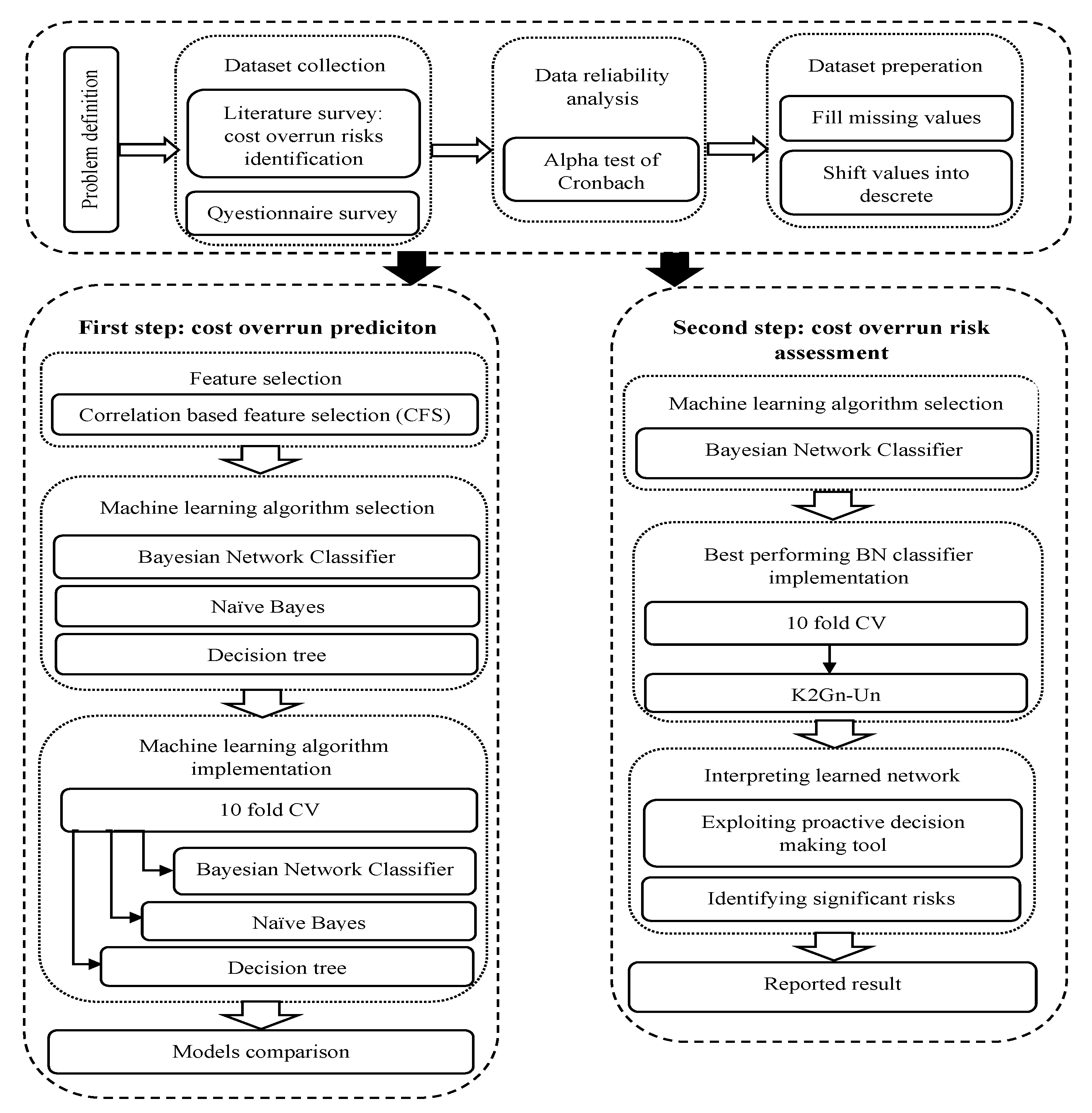
This study aims to predict cost overruns and assess the risk factors associated with cost overruns using an interpretable ML model that considers the potential relationships between the risks. To this end, and per the ML process, this study implemented ML models in two steps (Figure 1). The current study implemented three different ML algorithms and compared their performance accuracy in the first step using the feature selection step to predict cost overrun. This study examined the effect of considering possible relationships between cost overrun risks on the accuracy of cost overrun prediction in ML models at this stage. On the other hand, the second step’s objective was to assess the risk of cost overruns by interpreting the learned model and identifying all possible relationships between the risks. The model included all risks; the feature selection step was omitted. Additionally, this research presented a preventive decision-making tool to assist stakeholders in risk management by interpreting the learned model.

5.1. Data Collection

In the construction industry, data are collected in two ways: objective data from recorded reports on construction projects and subjective data from industry experts. While the methods for generating and collecting data in the construction industry have improved, the data may still not be stored in a way that facilitates knowledge extraction [21]. Unfortunately, objective data are challenging to obtain, as the construction industry is still chronically behind the curve when recording and publishing data suitable for ML applications [8]. Researchers have identified quantitative and qualitative factors associated with construction cost overruns. 43 cost overrun factors were identified in a literature review as appearing most frequently or in highly cited papers. These factors were gathered from seven research papers that addressed the cost overrun problem in construction projects. Then, on a 1–5 Likert scale, experts were asked to rate the probability and impact of the identified risks (1: very low, 2: low, 3: medium, 4: high, 5: very high). The experts were selected randomly by visiting the related organizations to the case study. One expert refused to answer the questionnaire. There were 41 experienced specialists involved in total. These individuals are involved in organizations representing employers, contractors, consultants, and project management (

Table 2. Respondents’ profile.

Category	Type	Number	Percent
Organization	Employer	10	25.6
	Consultant	9	23.1
	Contractor	11	28.2
	Consultant/Employer	3	7.7
	Consultant/Contractor	4	10.3
	Government supervisor	2	5.1
Experience (years)	=<20	13	33.3
	=<15	12	30.8
	=<10	11	28.2
	=<5	3	7.7
Discipline	Civil Engineering	33	84.6
	Architecture	3	7.7
	Electrical Engineering	2	5.1
	Industrial Engineering	1	2.6
Education level	Bachelor’s	20	51.3
	Master’s	17	43.6
	Ph.D.	2	5.1

). Two responses were excluded from the dataset due to their ineligibility: a lack of experience with construction projects and a high rate of missing data. Finally, 39 responses were qualified for the development of the dataset.

Table 3. Identified Risks’ Specifications.

No.	Source	Risk Factors	Reference	Code	Probability Impact
					Mean	Stdv.	Mean	Stdv.
1	Managerial	Poor feasibility study	[57]	Mg1	3.28	1.21	3.95	1.02
2		Contractor managerial weakness	[45,57]	Mg2	3.05	1.05	4.28	0.76
3		Poor communication between the parties	[45,58]	Mg3	2.59	0.68	3.28	1.02
4		Conflict between the project parties	[45]	Mg4	2.67	1.03	3.33	0.98
5		Consultant managerial weakness	[58]	Mg5	2.90	0.97	3.82	0.82
6		Owner incapable of project manager	[58]	Mg6	2.97	1.29	3.77	1.06
7	Materials and Equipment	Increased price of materials	[59]	Mt1	4.59	0.55	4.74	0.59
8		Shortage of equipment	[58]	Mt2	2.79	1.20	3.18	1.27
9		Delay by the suppliers in delivering equipment to the site	[45,58,60]	Mt3	2.74	1.04	3.23	1.13
10		Shortage of materials	[59]	Mt4	2.56	1.19	3.18	1.23
11		New equipment/technology issues	[61]	Mt5	2.23	1.20	2.69	1.19
12	Workforce	Lack of knowledge and experience	[45]	Hu1	2.74	0.88	3.28	1.02
13		Labour shortage	[45,60]	Hu2	2.18	1.10	3.26	1.07
14		Lack of skilled personnel (technical staff) on site	[45,60]	Hu3	2.61	1.14	3.56	1.05
15	Financial	Currency exchange rate	[59,60,61]	Fi1	4.20	1.13	4.49	0.91
16		Inflation	[59,61]	Fi2	4.69	0.52	4.85	0.36
17		Owner fund shortage and payment delays	[57,61]	Fi3	4.05	1.10	4.36	0.84
18		Multiple sources of funds	[57]	Fi4	2.54	1.00	3.13	1.15
19		Contractor fund shortage	[57]	Fi5	3.38	0.78	3.92	1.06
20	Project	Adverse change in geological conditions	[45,60]	Pr1	2.10	1.14	3.08	1.26
21		Site constraints	[45]	Pr2	2.23	1.01	2.69	1.05
22		Project complexity	[45,60]	Pr3	2.51	1.05	3.20	1.15
23	Owner	Site availability	[59]	Ow1	2.26	0.97	3	1.32
24		Change orders during construction	[58,59,60,61]	Ow2	3.44	1.16	3.77	0.96
25		Delays in decision making	[58]	Ow3	3.38	1.02	3.77	0.96
26		Owner customs policy and complexity (procurement delay)	[45]	Ow4	2.95	1.34	3.48	1.33
27		Delays in land acquisition	[58]	Ow5	2.54	1.21	3.28	1.39
28		Utility supply	[59]	Ow6	4.08	0.84	2.13	1.00
29		Lowest bidder selection	[41]	Ow7	3.67	1.11	3.74	1.12
30	Contractor	Lack of knowledge and experience	[45,59,60]	Cn1	3.20	0.92	3.85	0.93
31		Procurement delays	[45]	Cn2	2.85	0.84	3.54	0.91
32		Sub-contractor delays from preceding work	[60]	Cn3	3.05	0.97	3.33	1.06
33		Improper finance management	[41]	Cn4	3.15	1.09	3.77	0.90
34		Site safety	[45,59]	Cn5	2.979	1.22	3.38	1.39
35		Construction (defect) quality	[45,59]	Cn6	3.10	1.12	3.74	1.19
36		Poor planning and scheduling	[58]	Cn7	3.28	1.19	3.97	0.90
37	Consultant	Lack of knowledge and experience	[45,58]	Cs1	2.74	1.09	3.67	1.08
38		Improper design/design errors	[45,59,60]	Cs2	2.95	1.02	3.79	1.13
39		Delays in delivering design	[45,58]	Cs3	2.70	1.03	3.49	0.97
40		Change of equipment, or specification of equipment, during construction	[58]	Cs4	2.64	0.99	3.26	1.07
41	Environment	Bad weather or emergency condition	[45,57,58,59,61]	Ev1	2.64	0.93	3.28	0.94
42		Unexpected casualties/injuries	[59,60,61]	Ev2	1.77	1.01	2.36	1.33
43		Environment preservation law	[41]	Ev3	1.46	0.82	1.92	1.18

summarizes the risks identified and each risk’s average probability and impact, as determined by expert responses.

5.2. Data Reliability

The present study used the Alpha Test of Cronbach because several studies have used this method to check the validity of the results of questionnaires conducted by the Likert scale method (e.g., [23,24]). This method is used to assess the internal consistency of the questionnaire. Thus, as the internal consistency of the questionnaire increases, the alpha coefficient also increases, implying that if the questionnaire items have the most relevance to the target variable, this coefficient increases. The main purpose of the coefficient is to assess how accurate the data obtained from the survey are by evaluating the internal consistency coefficient of data. In addition, it was important to decide whether the combined factors help predict cost overrun [24]. Alpha of Cronbach can be written as:

$$\alpha =\frac{N}{\left(N-1\right)}\left(1-\frac{{{\displaystyle \sum }}_{i=1}^N{\sigma }_i^2}{{\sigma }_x^2}\right)$$

(1)

where N is the number of factors, ${\sigma }_i^2$ is the covariance between responses, and ${\sigma }_x^2$ is the variance of the sum of the answers. While there is no lower bound, the higher the Alpha coefficient of Cronbach is to 1, the greater the internal accuracy of the factors [62]. The findings of this study on the 43 factors resulted in Cronbach’s Alpha of 0.92, implying excellent internal consistency in the questionnaire, and the answers obtained from the questionnaire have high reliability.

5.3. Data Preparation and Preprocessing

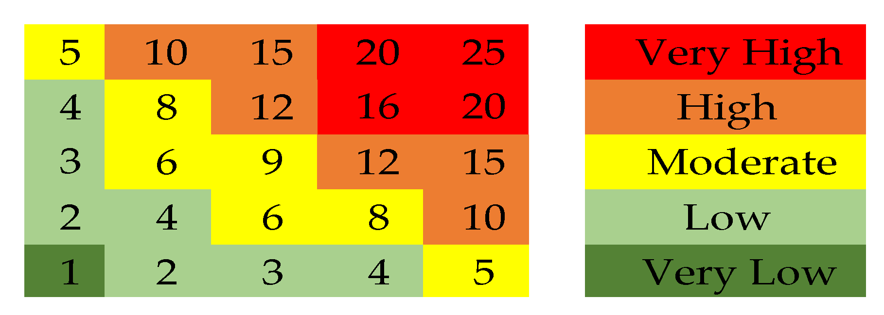
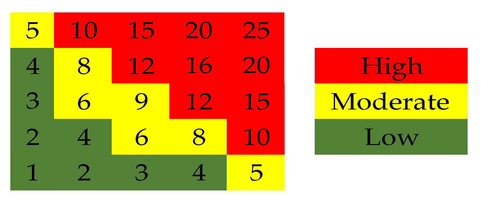
After collecting the data, the probability and impact of the risks were multiplied, and the magnitude of each risk was assigned to each response (Equation (2)) under the definition of risk magnitude in ISO 31000:2018. Then, for each sample, the values of the output variables were determined and quantified (Equation (3)), where n equals 43, the total number of identified risks. After specifying the dataset’s numerical values, the input and output variables were converted to nominal values using matrixes (4) (Figure 2) and (5) (Figure 3), respectively. Finally,

Table 4. Dataset.

Instance	Input Variables					Class
	Mg1	Mg2	Mg3	...	Ev3
1	Low	Low	Low	...	Very Low	Moderate
2	High	High	Moderate	...	Very Low	Moderate
3	Moderate	High	High	...	Very Low	Moderate
...	...	...	...	...	...	...
38	Very High	Very High	Moderate	...	Very Low	High
39	Very High	High	Moderate	...	Very Low	High

summarizes the research’s dataset, which is ready for ML models. Thus, 38.5% of the instances were classified as moderate-class, 61.5% as high-class, and none as low-class (

Table 5. Class label distribution.

Label	Number	Percent
Low	0	0
Moderate	15	38.5
High	24	61.5

). The first step involved applying the feature selection process following the research objectives. As a result, the Correlation-based Feature Selection (CFS) method was used in this study. The method’s central hypothesis is that good feature sets contain highly correlated features with the class but not one another. An operational definition of this hypothesis is provided by a feature evaluation formula based on concepts from test theory. CFS is an algorithm that combines this evaluation formula with an appropriate correlation measure and a heuristic search strategy to produce a heuristic search strategy. Hall [63] compared CFS to a wrapper—a well-known approach to feature selection that evaluates feature sets using the target learning algorithm. CFS produced results comparable to those of the wrapper in many cases and generally outperformed the wrapper on small datasets. Additionally, CFS executes faster than the wrapper, allowing it to scale to larger datasets.

$$\mathrm{Risk} \mathrm{Magnitude}\left(\mathrm{RM}1\right)= \mathrm{Probability} \times \mathrm{Impact}$$

(2)

$$\mathrm{Risk} \mathrm{Magnitude}\left(\mathrm{RM}2\right)=\sum \left(\mathrm{RM}1\right)/\mathrm{n}$$

(3)

5.4. Algorithm Selection: An Experimental Analysis

Algorithms in the genera category of ML algorithms must be defined concerning the collected data to select the optimal algorithm. Due to the labeled dataset, this research examined supervised algorithms. Then, learning algorithms from the supervised algorithms were selected based on the problem definition of developing an interpretable ML model that considers the possible relationships between risks. Therefore, the BN classifier, NB, and DT classifiers were used in this study. The BN classifier is capable of considering possible relationships between variables. Additionally, this is an interpretable model. Despite the method’s unique characteristics and its successful application to real-world problems [64], this algorithm has not been used in risk prediction and assessment in construction management literature. The NB classifier, which assumes independent variables, was developed to compare the results of cost overrun prediction with the BN classifier. This comparison enabled us to determine whether considering possible relationships between cost overrun risks affects the accuracy of cost overrun prediction in ML models. On the other hand, due to their widespread implementation in previous studies, both DT and NB models can be considered benchmark algorithms for evaluating the performance of the BN classifier model.

5.5. Decision Tree

The DT is a collection of ML algorithms used in statistical classification [65]. DTs are a subset of supervised learning algorithms, most of which are based on the objective of minimizing a function called entropy. There are, however, additional functions for learning the DT. Earlier models of the DT could only use discrete variables, but newer algorithms are capable of learning with both discrete and continuous variables. One of the significant advantages of the DT algorithm is its simplicity of comprehension and interpretation [66,67,68]. DTs are classified into two categories: ID3 and C4.5. ID3 can only learn from discrete variables. Conversely, C4.5 can learn from discrete and continuous variables [67]. J48 is a WEKA algorithm that generates pruned and unpruned C4.5. DTs may employ a variety of learning metrics. Entropy is one of the most frequently used metrics (information gain). Information gain $I_E$ is one of the DT learning metrics based on entropy and is formulated as follows:

$$H\left(T\right)=I_E\left(p_1,p_2,\dots ,p_J\right)=-{\displaystyle \sum }_{i-1}^J{p}_i{\log }_2 p_i$$

(4)

where $H\left(T\right)$ is entropy and p1, p2,$\dots$ denote fractions that sum to one and represent each class’s percentages in the child node after division. Therefore, the information gained is obtained in the system $IG\left(T,a\right)$ from the division of a node by subtracting the entropy of the system before and after the division (i.e., parent entropy $H\left(T\right)$ minus child entropy $H\left(T|a\right)$) as follows:

$$IG\left(T,a\right)=H\left(T\right)-H\left(T|a\right)=-{\displaystyle \sum }_{i=1}^J{p}_i{\log }_2{p}_i-{\displaystyle \sum }_{i=1}^J-Pr\left(i|a\right){\log }_{2}Pr\left(i|a\right)$$

(5)

Tree learning is the process of first determining which variable results in the greatest change in entropy (i.e., the greatest information gain) and then dividing the dataset according to this variable. This procedure is repeated for each newly created subcategory and continues until they achieve a certain level of purity [65]. As a result, the order of variables in a DT structure indicates the amount of information they contain.

5.6. Naïve Bayes

The NB classifier is a Bayesian-based statistical technique that determines an observation’s probability of belonging to a particular class. Using a training dataset, the technique calculates the prior probabilities of an observation occurring in a particular class within a predefined set of classes. Then, it employs the prior probabilities to determine the posterior probabilities that an observation belongs to each class. Finally, class membership is defined for a tested observation by selecting the most posterior probability class [21]. The NB can be considered a conditional probability model. Suppose $X=\left(x_1,\dots ,x_n\right)$ represents the vector of n attributes that are independent variables. Thus, the probability of encountering $C_k$ i.e., $p\left(C_k|x_1,\dots ,x_n\right)$, can be expressed as one of the states of various event classes for k as follows:

$$P\left(C_k|X\right)=\frac{P\left(X|C_k\right)P\left(C_k\right)}{P\left(X\right)}$$

(6)

As seen, Equation (6) is identical to the Bayesian theorem. Thus, to calculate the probability of $p\left(C_k|x_1,\dots ,x_n\right)$ it is sufficient to use the joint probability and simplify it using the conditional probability according to the variables’ independence:

$$p\left(C_k|x_1,\dots ,x_n\right)=p\left(x_1|x_2\dots ,x_n,C_k\right)p\left(x_2|x_3\dots ,x_n,C_k\right)p\left(x_n-1|x_n,C_k\right)p\left(C_k\right)$$

(7)

If the variables in x1 are assumed to be independent, the probabilities can be expressed more simply. Consider the following relation:

$$p\left(x_i|x_{i+1},\dots ,x_n,C_k\right)\approx p\left(x_i|C_k\right)$$

(8)

The probability can be expressed in this manner as a multiplication of the conditional probability:

$$p\left(C_k|x_1,\dots ,x_n\right)=p\left(C_k\right){\displaystyle \prod }_{i=1}^{n}p\left(x_i|C_k\right)$$

(9)

because the fraction’s denominator is constant throughout the calculation in relation (6), the conditional probability can be considered proportional to the combined probability. Given the preceding and the relation (9), the conditional probability presented in Equation (8) can be calculated as follows. As a result, the probability of an observation belonging to the category or group $C_k$ based on X observations is determined by the following relation:

$$p\left(C_k|x_1,\dots ,x_n\right)=\frac{1}{Z}p\left(C_k\right){\displaystyle \prod }_{i=1}^{n}p\left(x_i|C_k\right)$$

(10)

Only the output variable (child) is dependent on all of the input variables (parents) in the NB; there is no interdependence between the input variables.

5.7. Bayesian Network Classifier

Recent work in supervised learning has demonstrated that a surprisingly simple Bayesian classifier called NB, which makes strong assumptions about feature independence, is competitive with state-of-the-art classifiers such as C4.5. This fact leads to whether a classifier with less restrictive assumptions could perform even better [69]. BN classifiers are a subset of Bayesian networks that are optimized for classification problems. These classifiers have several advantages, including model interpretation, compliance with complex data and classification problem environments, efficient learning and classification algorithms, and successful application to real-world problems [64].

Consider the following set of variables. On a set of variables U, BN B is a directed acyclic network structure with B_S on it, as well as a collection of possible tables. where pa(u) is u’s parent set in assumptions: Each variable is discrete and finite, and no data are missing. The BN algorithm is implemented in B_S. BN provides probable distributions P_U = Qu∈U p(u|pa(u)). WEKA’s BN algorithms start with two steps: first, the network structure must be learned, followed by the probability tables. After determining an appropriate network structure, conditional probability tables for each variable can be estimated [70].

This research built 18 BNs to determine the optimal network among them. The learning algorithm, network type, and the maximum number of parents differ between these networks. In general, three types of learning algorithms: K2, hill-climbing, and tabu search; two types of networks: InitAsNaiveBayes and General; and three modes for the maximum number of parents, 2, 3, and None, were considered.

5.7.1. Learning Bayesian Networks

A learning algorithm for BNs is constructed by defining two components: a function for evaluating a given network against the available data and a method for searching through the space of possible networks. The quality of a network is determined by the probability of the data it transmits.

K2, a fast and straightforward learning algorithm, begins with a predefined ordering of the attributes (i.e., nodes). Then it processes each node in turn, greedily considering adding edges to the current node from previously processed nodes. Each step maximizes the network’s score by adding an edge. Attention is directed to the next node when no further improvement is apparent.

A more sophisticated but slower version of K2 is hill-climbing, which considers adding or deleting edges between arbitrary pairs of nodes without regard for order. Additionally, consider inverting the direction of existing edges. As with any greedy algorithm, the resulting network only represents a local maximum of the scoring function: it is always prudent to run such algorithms multiple times with different random initial configurations.

Furthermore, more sophisticated optimization techniques, such as tabu search, can be used [49]. Tabu search performs hill-climbing until it reaches a local optimum. Then it steps to the least worse candidate in the neighborhood. However, it does not consider points in the neighborhood it just visited in the last tl steps. These steps are stored in a so-called tabu-list [71].

5.7.2. Network Type

There are two types of BN classifiers in general. These two networks are created in WEKA using the initAsNaiveBayes criterion. The first is when initAsNaiveBayes is set to True.

The primary network structure used to search the search space, in this case, is a simple NB structure. In this case, a structure is created by connecting the class variable to each feature variable via an arrow. This kind is referred to as an initAsNaiveBayes network. The other possibility is when initAsNaiveBayes is set to False. In this case, the primary network structure is an empty network. This state is referred to as General in this study.

5.7.3. Maximum Number of Parents

This is an upper bound on the number of parents of each node in the learned network structure. This research examined three modes: 2, 3, and None. This value is specified in WEKA using the maxNrOfParents criterion. When the network type initAsNaiveBayes is selected, setting this parameter to 2 results in a Tree Augmented Naive Bayes (TAN) network. Similarly, specifying number 3 results in a Bayesian Network Augmented Naive Bayes (BAN). By setting it to a significantly greater than the number of network nodes (100,000 almost guarantees this), no restriction on the number of parents is imposed. The final mode is referred to as None in this study, and the network created in this manner is referred to as Un, which stands for Unlimited.

5.8. Training and Evaluation Method and Performance Metrics

This study used the k-fold CV method to train and evaluate models because it uses the entire data set for training and testing, unlike the hold-out method. The present study considered a 10-fold CV because numerous studies have indicated that this is the optimal value for computational time, error estimation, and indices variance [22]. Five performance metrics were selected for evaluation to show the model’s performance comprehensively, accuracy, the area under ROC, precision, recall, and f1-score. The precision and recall indices are appropriate when there is an unbalanced distribution of classes, which is the case in the present study. Before proceeding to model performance metrics, a few key terms for each class need to be clarified first [22]:

• True positives (TPs): Number of predictions that were correctly assigned to a class (i.e., value in the matrix diagonal for the corresponding class).
• False positives (FPs): Number of predictions that were incorrectly assigned to a class (i.e., the sum of values in the corresponding class column excluding the TPs).
• False negatives (FNs): Number of predictions incorrectly unrecognized as class assignments (i.e., the sum of values in the corresponding class row excluding the TPs).
• True negatives (TNs): Number of predictions correctly recognized as not belonging to a class (i.e., the sum of values of all rows and columns excluding the row and column of that class).

$$accuracy=\frac{TP+TN}{TP+FN+FP+TN}$$

(11)

$$precision=\frac{TP}{TP+FP}$$

(12)

$$recall=\frac{TP}{TP+FN}$$

(13)

$$F1-score=2\times \frac{precision\times recall}{precision+recall}$$

(14)

6. Results

6.1. Models Implementation

The current study implemented the identified algorithms in two distinct steps to meet the research objectives. In the first step, 18 BN classifiers, NB, and DT, were implemented to predict cost overrun, and the results were compared. This comparison demonstrates the effect of considering the relationships between cost overrun risks on the predictive accuracy of cost overruns in ML models. The second step involved implementing the best BN classifier identified in the first step without using the feature selection method. The purpose of including all risks in the second step was to establish relationships between them and to create a comprehensive, proactive decision-making tool.

6.2. First Step: Cost Overrun Prediction

At this stage, 18 different BN classifiers, NB and DT, along with the CFS feature selection stage, have been implemented to predict the cost increase. Furthermore, from the results of this step and comparing the performance metrics of the mentioned models, the best model can be identified and implemented to analyze the risks of cost overrun in the second step.

In this study, five performance metrics, accuracy, area under ROC curve, precision, recall, and F1-score, have been selected to compare the performance of algorithms.

Table 6. Models performance.

Name	Learning Algorithm	Network Type	Max. Num. of Parents	Accuracy	Area under ROC	Precision	Recall	F1-Score
K2-TAN	K2	initAsNaive Bayes	2	80.25	0.89	0.87	0.80	0.83
K2-BAN		initAsNaive Bayes	3	79.75	0.89	0.86	0.80	0.83
K2-Un		initAsNaive Bayes	None	79.75	0.89	0.86	0.80	0.83
K2GN-2		General	2	80.25	0.90	0.87	0.80	0.83
K2GN-3		General	3	79.75	0.89	0.86	0.80	0.83
K2GN-Un		General	None	79.75	0.89	0.86	0.80	0.83
HC-TAN	hill-climbing	initAsNaive Bayes	2	79.25	0.89	0.86	0.79	0.82
HC-BAN		initAsNaive Bayes	3	79	0.88	0.86	0.79	0.82
HC-Un		initAsNaive Bayes	None	79	0.88	0.86	0.79	0.82
HCGN-2		General	2	77.75	0.88	0.84	0.78	0.81
HCGN-3		General	3	77.50	0.88	0.84	0.78	0.81
HCGN-Un		General	None	77.50	0.88	0.84	0.78	0.81
TS-TAN	tabu search	initAsNaive Bayes	2	79.25	0.88	0.86	0.79	0.82
TS-BAN		initAsNaive Bayes	3	78.75	0.88	0.85	0.79	0.82
TS-Un		initAsNaive Bayes	None	78.75	0.88	0.85	0.79	0.82
TSGN-2		General	2	77.75	0.90	0.85	0.78	0.81
TSGN-3		General	3	77.75	0.90	0.85	0.78	0.81
TSGN-Un		General	None	77.75	0.90	0.85	0.78	0.81
BN classifier models (average)				78.86	0.89	0.85	0.79	0.82
NB				77.92	0.89	0.85	0.78	0.81
DT				65.25	0.68	0.76	0.65	0.70

compares the performance of the developed models. The results of implementing the algorithms in the first step show that the average performance accuracy of 18 BN classifiers is 78.86%, which is higher than the accuracy of NB at 77.92% and DT at 65.25%. The best models for this stage are K2-TAN and K2GN-2, with excellent performance accuracy of 80.25. In the area under the ROC curve, the average of 18 BN classifiers and NB is equal to 0.89, and DT shows a performance of 0.68.

Despite being faster and more straightforward than the hill-climbing and tabu search methods, the K2 algorithm performed well among BN learning algorithms (Table 6).

Thus, it can be concluded that the BN classifier can be used as a robust learning algorithm to predict cost overruns in construction projects while making reasonable assumptions about the relationship between risks. Moreover, considering possible relationships between cost overrun risks improves the ML model’s cost overrun prediction accuracy for construction projects.

6.3. Second Step: Cost Overrun Risk Analysis

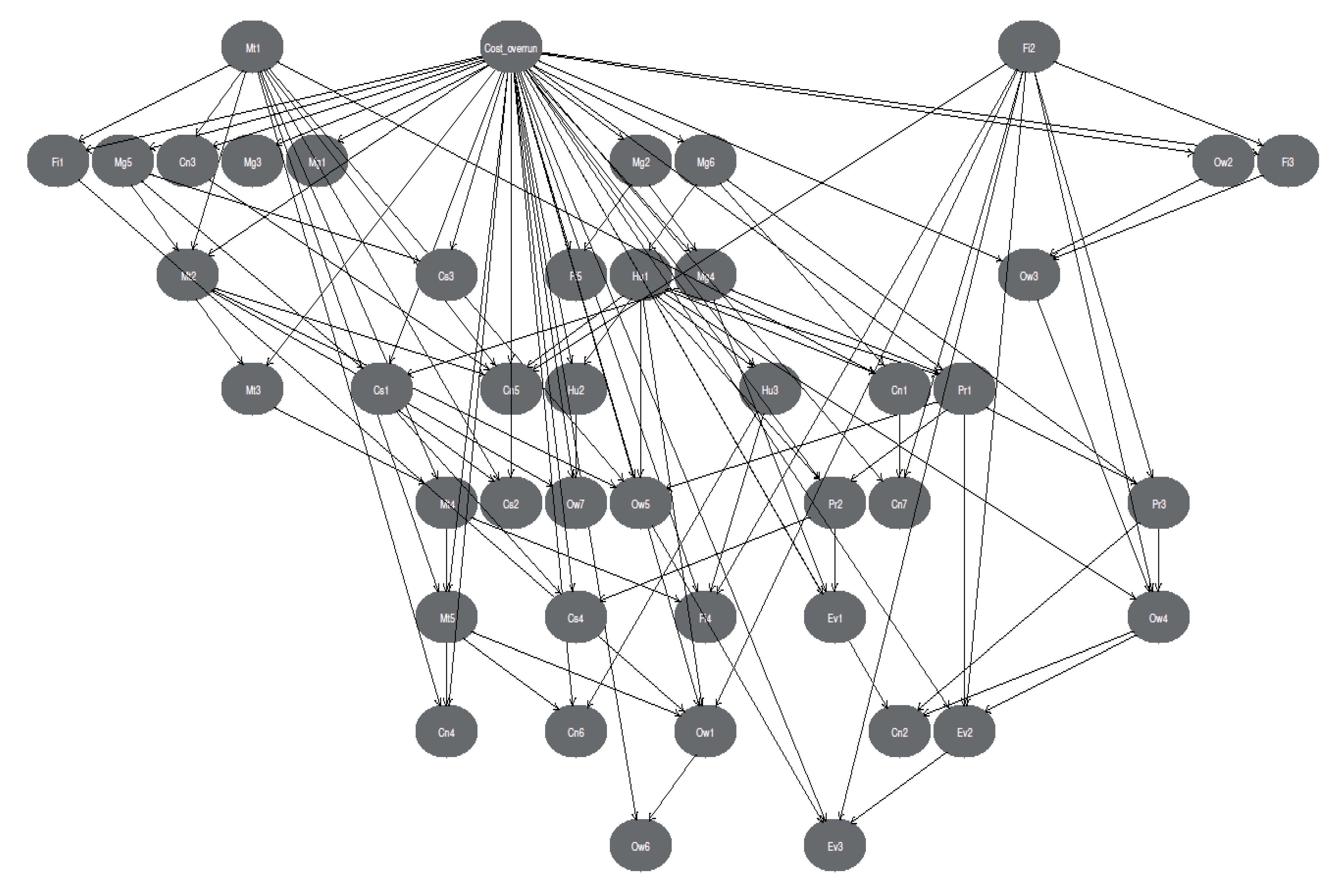
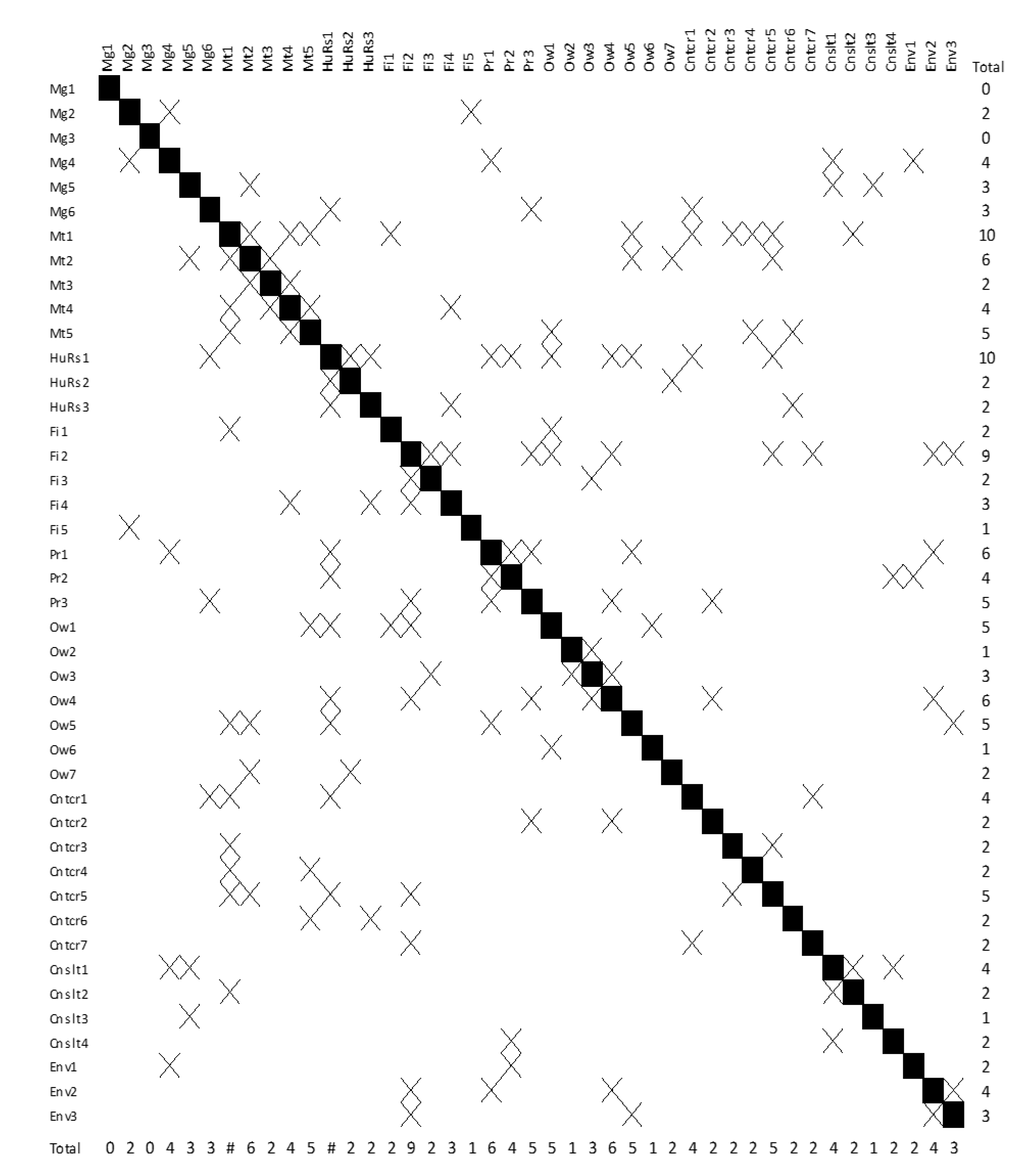
The second step aims to analyze the risks of cost overrun by interpreting the learned model. Therefore, the feature selection step was omitted to develop a comprehensive model to analyze all the risks. This feature allows risk relationships to be fully defined without any limits. Furthermore, a model should be chosen that imposes no constraints on modeling. Among K2GN- Un, HCGN-Un, and TSGN-Un, which lacked a cap on the maximum number of parents and the creation of the first network, the K2GN-Un model was chosen to determine the relationships between cost overrun risks due to its simplicity, speed, and high accuracy. A noteworthy point during this stage was that the model’s performance was improved despite the absence of a feature selection stage, implying that including all cost overrun risks in the BN classifier improves cost overrun prediction performance (

Table 7. K2GN-Un accuracy without the feature selection step.

Metrics	Performance
Accuracy	81.67
Area Under ROC	0.93
Precision	0.89
Recall	0.82
F1-score	0.84

). This study used the learned BN (Figure 4) to establish relationships between cost overrun risks (Figure 5). This enabled us to introduce a proactive decision-making tool to assist the risk management process (Figure 5). Additionally, this study identified the most critical construction cost overrun risks based on the number of relationships (

Table 8. Most critical risks.

Rank	Risk	Number of Connections
1	Increased price of materials	10
2	Lack of knowledge and experience	10
3	Inflation	9
4	Owner customs policy and complexity (procurement delay)	6
5	Shortage of equipment	6
6	Adverse change in geological conditions	6
7	Construction (defect) quality	5
8	Project complexity	5
9	Delays in land acquisition	5
10	Site availability	5

). The increased price of materials, lack of knowledge and experience, and inflation were identified as the most critical risks regarding the number of relationships with other risks.

7. Discussion

This study trained and evaluated ML models by the 10-fold CV in both steps. The results obtained in the first step from implementing 18 different BN classifiers using the CFS feature selection method demonstrated that all 18 models performed satisfactorily, with the K2Gn-Un model performing at 80.25% and 0.8 WROC index. The study compared this research model to recently implemented models in comparable fields with similar performance metrics to give an overview of the literature’s models (

Table 9. Compared studies.

Study	Best Model	Performance
Gondia et al. [22]	NB	Accuracy: 78.4%
Ghazal and Hammad [21]	RF	Accuracy: 65.22%
Egwim et al. [24]	Gaussian NB	Area under ROC: 0.74

). However, this comparison does not imply the proposed model’s performance superiority over previous studies due to different datasets being used. For instance, in a Gondia et al. [22] study, the best ML model was the NB, which had a 51.2% accuracy rate. Additionally, according to research by Ghazal and Hammad [21], the best ML model was the random forest, with an accuracy of 65.22% and a WROC index of 0.76. In another study by Egwim et al. [24], the best model was Gaussian naive Bayes with an area under ROC of 0.74. In this study, the 18 BN classifiers predict cost overruns with a higher degree of accuracy than those reported in previous research. This ML model can potentially be a highly effective tool for predicting cost overruns in construction projects, as it makes more realistic assumptions about the relationships between risks than other models. The current study interpreted the BN classifier’s learned model to aid in proactive decision-making in risk management. This study implemented the second step of executing the BN classifier for this purpose. The K2Gn-Un model was implemented because it was the best-performing unrestricted model identified in the first step. Surprisingly, the model’s accuracy and WRC index increased by about 2% and 4% in the second step, respectively, despite the absence of the feature selection stage. This increased prediction accuracy demonstrates the importance of considering all cost overrun risks when predicting cost overruns in construction projects.

The distinction to be made is between correlation and causation. Causation is often inferred from networks that human experts construct. These networks are usually straightforward and have few parameters. However, when ML techniques are applied to induce models from data whose causal structure is unknown, they can construct a network based on the correlations observed in the data [49].

This study interpreted the learned K2Gn-Un network, which resulted in developing a tool that assists project stakeholders in making preventive decisions. Figure 5 demonstrates the direct correlations between cost overrun risks and the total number of relationships extracted from the learned network for each risk. This table can be used as a tool to determine the impact of various risks on other risks before their occurrence. Additionally, the outcomes are used to identify ten critical risks based on the total number of relationships with other risks.

Finally, the novelties of this study are summarized in the following:

• Utilizing the BN classifier model to predict cost overruns and assess cost overrun risks for the first time in construction management
• Evaluating the effect of considering possible relationships between cost overrun risks on the predictive accuracy of cost overruns in construction projects in ML models
• Determining the correlations between cost overrun risks and identifying the most critical cost overrun risks in terms of the number of relationships with other risks by interpreting the learned BN classifier model.
• Developing a proactive decision-making tool to assist stakeholders with risk management.

8. Conclusions

Cost overrun is a significant challenge in construction projects due to its dynamic, complex nature and the possible interrelationships between cost overrun risks. This problem is mitigated by considering relationships between cost overrun risks in the risk assessment process. The current study proposes an ML approach based on the BN classifier algorithm to predict cost overruns and assess the associated risks. Considering the possible relationships between the input variables—cost overrun risks—and interpretability are two significant advantages of this model. Two distinct steps were taken to implement the BN classifier. The first step was to implement the BN classifier, NB classifier, and DT for cost overrun prediction and their performance comparison. This step applied the CFS feature selection step to all models. This step revealed that the average prediction accuracy of the 18 BNs classifiers was 78.86%, which is higher than the NB and DT classifiers. Additionally, this stage demonstrated that considering possible relationships between cost overrun risks improves the ML model’s cost overrun prediction accuracy for construction projects. In the second step, the best BN model was implemented for cost overrun risk analysis. The model was implemented without feature selection to analyze relationships between all the risks, and the learned model was interpreted. The second step results demonstrated that the BN classifier, which includes all cost overrun risks, outperforms the model with selected risks in cost overrun prediction accuracy. Moreover, this study developed a proactive decision-making tool capable of assisting the risk management process by interpreting the learned model at the second stage. This tool established direct correlations between all risks and identified the most critical risks based on the number of correlations between them. As a result of this research, the most significant risks are identified as the increased price of materials, lack of knowledge and experience among human resources, and inflation.

References

- Afzal, F.; Yunfei, S.; Nazir, M.; Bhatti, S.M. A review of artificial intelligence based risk assessment methods for capturing complexity-risk interdependencies: Cost overrun in construction projects. Int. J. Manag. Proj. Bus. 2019, 14, 300–328. [Google Scholar] [CrossRef]
- Shane, J.S.; Molenaar, K.R.; Anderson, S.; Schexnayder, C. Construction project cost escalation factors. J. Manag. Eng. 2009, 25, 221–229. [Google Scholar] [CrossRef]
- Hammad, A.; AbouRizk, S.; Mohamed, Y. Application of KDD techniques to extract useful knowledge from labor resources data in industrial construction projects. J. Manag. Eng. 2014, 30, 5014011. [Google Scholar] [CrossRef]
- Liu, J.; Zhao, X.; Yan, P. Risk paths in international construction projects: Case study from Chinese contractors. J. Constr. Eng. Manag. 2016, 142, 5016002. [Google Scholar] [CrossRef]
- Love, P.E.; Ahiaga-Dagbui, D.D.; Irani, Z. Cost overruns in transportation infrastructure projects: Sowing the seeds for a probabilistic theory of causation. Transp. Res. Part A Policy Pract. 2016, 92, 184–194. [Google Scholar] [CrossRef] [Green Version]
- Darko, A.; Chan, A.P.; Adabre, M.A.; Edwards, D.J.; Hosseini, M.R.; Ameyaw, E.E. Artificial intelligence in the AEC industry: Scientometric analysis and visualization of research activities. Autom. Constr. 2020, 112, 103081. [Google Scholar] [CrossRef]
- García de Soto, B.; Agustí-Juan, I.; Joss, S.; Hunhevicz, J. Implications of Construction 4.0 to the workforce and organizational structures. Int. J. Constr. Manag. 2022, 22, 205–217. [Google Scholar] [CrossRef]
- Sanni-Anibire, M.O.; Zin, R.M.; Olatunji, S.O. Machine learning model for delay risk assessment in tall building projects. Int. J. Constr. Manag. 2020, 22, 2134–2143. [Google Scholar] [CrossRef]
- Jin, R.; Zuo, J.; Hong, J. Scientometric review of articles published in ASCE’s journal of construction engineering and management from 2000 to 2018. J. Constr. Eng. Manag. 2019, 145, 06019001. [Google Scholar] [CrossRef]
- Patrício, D.I.; Rieder, R. Computer vision and artificial intelligence in precision agriculture for grain crops: A systematic review. Comput. Electron. Agric. 2018, 153, 69–81. [Google Scholar] [CrossRef]
- Salehi, H.; Burgueño, R. Emerging artificial intelligence methods in structural engineering. Eng. Struct. 2018, 171, 170–189. [Google Scholar] [CrossRef]
- Islam, M.S.; Nepal, M.P.; Skitmore, M.; Attarzadeh, M. Current research trends and application areas of fuzzy and hybrid methods to the risk assessment of construction projects. Adv. Eng. Inform. 2017, 33, 112–131. [Google Scholar] [CrossRef]
- Hegde, J.; Rokseth, B. Applications of machine learning methods for engineering risk assessment—A review. Saf. Sci. 2020, 122, 104492. [Google Scholar] [CrossRef]
- Guide, A. Project Management Body of Knowledge (Pmbok® Guide); Project Management Institute: Newton Square, PA, USA, 2021. [Google Scholar]
- Soibelman, L.; Kim, H. Generating construction knowledge with knowledge discovery in databases. Comput. Civ. Build. Eng. 2000, 2, 906–913. [Google Scholar]
- An, S.-H.; Park, U.-Y.; Kang, K.-I.; Cho, M.-Y.; Cho, H.-H. Application of support vector machines in assessing conceptual cost estimates. J. Comput. Civ. Eng. 2007, 21, 259–264. [Google Scholar] [CrossRef]
- Lee, S.; Kim, C.; Park, Y.; Son, H.; Kim, C. Data Mining-Based Predictive Model to Determine Project Financial Success using Project Definition Parameters. In Proceedings of the 28th International Symposium on Automation and Robotics in Construction, ISARC, Seoul, Korea, 29 June–2 July 2011. [Google Scholar]
- Chaovalitwongse, W.A.; Wang, W.; Williams, T.; Chaovalitwongse, P. Data mining framework to optimize the bid selection policy for competitively bid highway construction projects. J. Constr. Eng. Manag. 2012, 138, 277–286. [Google Scholar] [CrossRef]
- Asadi, A.; Alsubaey, M.; Makatsoris, C. A machine learning approach for predicting delays in construction logistics. Int. J. Adv. Logist. 2015, 4, 115–130. [Google Scholar] [CrossRef]
- El-Kholy, A. Exploring the best ANN model based on four paradigms to predict delay and cost overrun percentages of highway projects. Int. J. Constr. Manag. 2021, 21, 694–712. [Google Scholar] [CrossRef]
- Ghazal, M.M.; Hammad, A. Application of knowledge discovery in database (KDD) techniques in cost overrun of construction projects. Int. J. Constr. Manag. 2020, 22, 1632–1646. [Google Scholar] [CrossRef]
- Gondia, A.; Siam, A.; El-Dakhakhni, W.; Nassar, A.H. Machine learning algorithms for construction projects delay risk prediction. J. Constr. Eng. Manag. 2020, 146, 4019085. [Google Scholar] [CrossRef]
- Yaseen, Z.M.; Ali, Z.H.; Salih, S.Q.; Al-Ansari, N. Prediction of risk delay in construction projects using a hybrid artificial intelligence model. Sustainability 2020, 12, 1514. [Google Scholar] [CrossRef]
- Egwim, C.N.; Alaka, H.; Toriola-Coker, L.O.; Balogun, H.; Sunmola, F. Applied artificial intelligence for predicting construction projects delay. Mach. Learn. Appl. 2021, 6, 100166. [Google Scholar] [CrossRef]
- Shoar, S.; Chileshe, N.; Edwards, J.D. Machine learning-aided engineering services’ cost overruns prediction in high-rise residential building projects: Application of random forest regression. J. Build. Eng. 2022, 50, 104102. [Google Scholar] [CrossRef]
- Dang-Trinh, N.; Duc-Thang, P.; Cuong, T.N.-N.; Duc-Hoc, T. Machine learning models for estimating preliminary factory construction cost: Case study in Southern Vietnam. Int. J. Constr. Manag. 2022, 1–9. [Google Scholar] [CrossRef]
- Bu-Qammaz, A.S.; Dikmen, I.; Birgonul, M.T. Risk assessment of international construction projects using the analytic network process. Can. J. Civ. Eng. 2009, 36, 1170–1181. [Google Scholar] [CrossRef]
- Taroun, A. Towards a better modelling and assessment of construction risk: Insights from a literature review. Int. J. Proj. Manag. 2014, 32, 101–115. [Google Scholar] [CrossRef]
- Huang, C.-N.; Liou, J.J.; Chuang, Y.-C. A method for exploring the interdependencies and importance of critical infrastructures. Knowl. -Based Syst. 2014, 55, 66–74. [Google Scholar] [CrossRef]
- Valipour, A.; Yahaya, N.; Noor, N.M.; Kildienė, S.; Sarvari, H.; Mardani, A. A fuzzy analytic network process method for risk prioritization in freeway PPP projects: An Iranian case study. J. Civ. Eng. Manag. 2015, 21, 933–947. [Google Scholar] [CrossRef] [Green Version]
- Pehlivan, S.; Öztemir, A.E. Integrated risk of progress-based costs and schedule delays in construction projects. Eng. Manag. J. 2018, 30, 108–116. [Google Scholar] [CrossRef]
- Gupta, V.K.; Thakkar, J.J. A quantitative risk assessment methodology for construction project. Sādhanā 2018, 43, 116. [Google Scholar] [CrossRef] [Green Version]
- Chandra, H.P. Structural equation model for investigating risk factors affecting project success in Surabaya. Procedia Eng. 2015, 125, 53–59. [Google Scholar] [CrossRef]
- Adeleke, A.Q.; Bahaudin, A.Y.; Kamaruddeen, A.M.; Bamgbade, J.A.; Salimon, M.G.; Khan, M.W.A.; Sorooshian, S. The influence of organizational external factors on construction risk management among Nigerian construction companies. Saf. Health Work. 2018, 9, 115–124. [Google Scholar] [CrossRef] [PubMed]
- Hung, L. A risk assessment framework for construction project using artificial neural network. J. Sci. Technol. Civ. Eng. 2018, 12, 51–62. [Google Scholar]
- Carr, V.; Tah, J. A fuzzy approach to construction project risk assessment and analysis: Construction project risk management system. Adv. Eng. Softw. 2001, 32, 847–857. [Google Scholar] [CrossRef]
- Taylan, O.; Bafail, A.O.; Abdulaal, R.M.; Kabli, M.R. Construction projects selection and risk assessment by fuzzy AHP and fuzzy TOPSIS methodologies. Appl. Soft Comput. 2014, 17, 105–116. [Google Scholar] [CrossRef]
- Prascevic, N.; Prascevic, Z. Application of fuzzy AHP for ranking and selection of alternatives in construction project management. J. Civ. Eng. Manag. 2017, 23, 1123–1135. [Google Scholar] [CrossRef] [Green Version]
- Shariat, R.; Roozbahani, A.; Ebrahimian, A. Risk analysis of urban stormwater infrastructure systems using fuzzy spatial multi-criteria decision making. Sci. Total Environ. 2019, 647, 1468–1477. [Google Scholar] [CrossRef]
- Ebrahimnejad, S.; Mousavi, S.; Tavakkoli-Moghaddam, R.; Hashemi, H.; Vahdani, B. A novel two-phase group decision making approach for construction project selection in a fuzzy environment. Appl. Math. Model. 2012, 36, 4197–4217. [Google Scholar] [CrossRef]
- Islam, M.S.; Nepal, M.; Skitmore, M. Modified fuzzy group decision-making approach to cost overrun risk assessment of power plant projects. J. Constr. Eng. Manag.-ASCE 2019, 145, 40181261-15. [Google Scholar] [CrossRef]
- Velasquez, M.; Hester, P.T. An analysis of multi-criteria decision making methods. International journal of operations research 2013, 10, 56–66. [Google Scholar]
- Aburrous, M.; Hossain, M.A.; Dahal, K.; Thabtah, F. Predicting Phishing Websites Using Classification Mining Techniques with Experimental Case Studies. In Proceedings of the 2010 Seventh International Conference on Information Technology: New Generations, Las Vegas, NV, USA, 12–14 April 2010; IEEE: Manhattan, NY, USA, 2010. [Google Scholar]
- Flath, C.; Nicolay, D.; Conte, T.; van Dinther, C.; Filipova-Neumann, L. Cluster analysis of smart metering data. Bus. Inf. Syst. Eng. 2012, 4, 31–39. [Google Scholar] [CrossRef]
- Eybpoosh, M.; Dikmen, I.; Birgonul, M.T. Identification of risk paths in international construction projects using structural equation modeling. J. Constr. Eng. Manag. 2011, 137, 1164–1175. [Google Scholar] [CrossRef]
- El-Sayegh, S.M. Risk assessment and allocation in the UAE construction industry. Int. J. Proj. Manag. 2008, 26, 431–438. [Google Scholar] [CrossRef]
- Guan, L.; Liu, Q.; Abbasi, A.; Ryan, M.J. Developing a comprehensive risk assessment model based on fuzzy Bayesian belief network (FBBN). J. Civ. Eng. Manag. 2020, 26, 614–634. [Google Scholar] [CrossRef]
- Yan, H.; Yang, N.; Peng, Y.; Ren, Y. Data mining in the construction industry: Present status, opportunities, and future trends. Autom. Constr. 2020, 119, 103331. [Google Scholar] [CrossRef]
- Witten, I.H.; Frank, E.; Hall, M.A. Data Mining: Practical Machine Learning Tools and Techniques; Morgan Kaufmann: San Francisco, CA, USA, 2005. [Google Scholar]
- Hu, Y.; Wang, Y.; Zhao, T.; Phoon, K.-K. Bayesian supervised learning of site-specific geotechnical spatial variability from sparse measurements. ASCE-ASME J. Risk Uncertain. Eng. Syst. Part A Civ. Eng. 2020, 6, 4020019. [Google Scholar] [CrossRef]
- Ayodele, T.O. Types of machine learning algorithms. New Adv. Mach. Learn. 2010, 3, 19–48. [Google Scholar]
- Fan, C.-L. Defect risk assessment using a hybrid machine learning method. J. Constr. Eng. Manag. 2020, 146, 04020102. [Google Scholar] [CrossRef]
- Brownlee, J. Why Data Preparation is so Important in Machine Learning. 2020. Available online: https://machinelearningmastery.com/data-preparation-is-important/ (accessed on 31 July 2022).
- Brownlee, J. Framework for Data Preparation Techniques in Machine Learning. 2020. Available online: https://machinelearningmastery.com/framework-for-data-preparation-for-machine-learning/ (accessed on 18 July 2021).
- Langley, P. Machine learning as an experimental science. Mach. Learn. 1988, 3, 5–8. [Google Scholar] [CrossRef] [Green Version]
- Mehrjoo, M. What to Consider before Selecting a Machine Learning Algorithm. 2017. Available online: https://www.linkedin.com/pulse/what-consider-before-selecting-machine-learning-marzieh-mehrjoo-phd (accessed on 18 July 2021).
- Ebrahimnejad, S.; Mousavi, S.; Mojtahedi, S. A Model for Risk Evaluation in Construction Projects Based on Fuzzy MADM. In Proceedings of the 2008 4th IEEE International Conference on Management of Innovation and Technology, Bangkok, Thailand, 21–24 September 2008; IEEE: Manhattan, NY, USA, 2008. [Google Scholar]
- Liu, J.; Xie, Q.; Xia, B.; Bridge, A.J. Impact of design risk on the performance of design-build projects. J. Constr. Eng. Manag.-ASCE 2017, 143, 40170101-10. [Google Scholar] [CrossRef]
- Ke, Y.; Wang, S.; Chan, A.P.; Lam, P.T. Preferred risk allocation in China’s public–private partnership (PPP) projects. Int. J. Proj. Manag. 2010, 28, 482–492. [Google Scholar] [CrossRef]
- Rebeiz, K.S. Public–private partnership risk factors in emerging countries: BOOT illustrative case study. J. Manag. Eng. 2012, 28, 421–428. [Google Scholar] [CrossRef]
- Li, Y.; Wang, X. Risk assessment for public–private partnership projects: Using a fuzzy analytic hierarchical process method and expert opinion in China. J. Risk Res. 2018, 21, 952–973. [Google Scholar] [CrossRef]
- Gliem, J.A.; Gliem, R.R. Calculating, Interpreting, and Reporting Cronbach’s Alpha Reliability Coefficient for Likert-Type Scales; Midwest Research-to-Practice Conference in Adult, Continuing, and Community: DeKalb, IL, USA, 2003. [Google Scholar]
- Hall, M.A. Correlation-Based Feature Selection for Machine Learning. Ph.D. Dissertation, The University of Waikato, Hamilton, New Zealand, 1999. [Google Scholar]
- Bielza, C.; Larranaga, P. Discrete Bayesian network classifiers: A survey. ACM Comput. Surv. (CSUR) 2014, 47, 1–43. [Google Scholar] [CrossRef]
- Provost, F.; Fawcett, T. Data Science for Business: What you Need to Know about Data Mining and Data-Analytic Thinking; O’Reilly Media, Inc.: Sebastopol, CA, USA, 2013. [Google Scholar]
- Hastie, T.; Tibshirani, R.; Friedman, J. The Elements of Statistical Learning: Data Mining, Inference and Prediction; Springer: New York, NY, USA, 2009. [Google Scholar]
- Piryonesi, S.M.; El-Diraby, T.E. Data analytics in asset management: Cost-effective prediction of the pavement condition index. J. Infrastruct. Syst. 2020, 26, 4019036. [Google Scholar] [CrossRef]
- Wu, X.; Kumar, V.; Ross Quinlan, J.; Ghosh, J.; Yang, Q.; Motoda, H.; McLachlan, G.J.; Ng, A.; Liu, B.; Yu, P.S. Top 10 algorithms in data mining. Knowl. Inf. Syst. 2008, 14, 1–37. [Google Scholar] [CrossRef] [Green Version]
- Friedman, N.; Geiger, D.; Goldszmidt, M. Bayesian network classifiers. Mach. Learn. 1997, 29, 131–163. [Google Scholar] [CrossRef]
- Bouckaert, R.R.; Eibe, F.; Hall, M.; Kirkby, R.; Reutemann, P.; Seewald, A.; Scuse, S. WEKA Manual for Version 3-9-1; University of Waikato: Hamilton, New Zealand, 2016. [Google Scholar]
- Bouckaert, R.R. Bayesian Network Classifiers in WEKA for Version 3-5-7; Artificial Intelligence Tools; University of Waikato: Hamilton, New Zealand, 2008; Volume 11, pp. 369–387. [Google Scholar]
Figure 1.
Methodology for developing the proposed cost overrun prediction and cost overrun risk assessment model.
Figure 2.
5 Classes Matrix Matrix.
Figure 3.
3 Classes Matrix Matrix.
Figure 4.
K2GN-Un learned network.
Figure 5.
Relationships between risks.