
Shear Strength Prediction of Slender Steel Fiber Reinforced Concrete Beams Using a Gradient Boosting Regression Tree Method

 , and
, and
Abstract
:1. Introduction
2. Materials and Methods
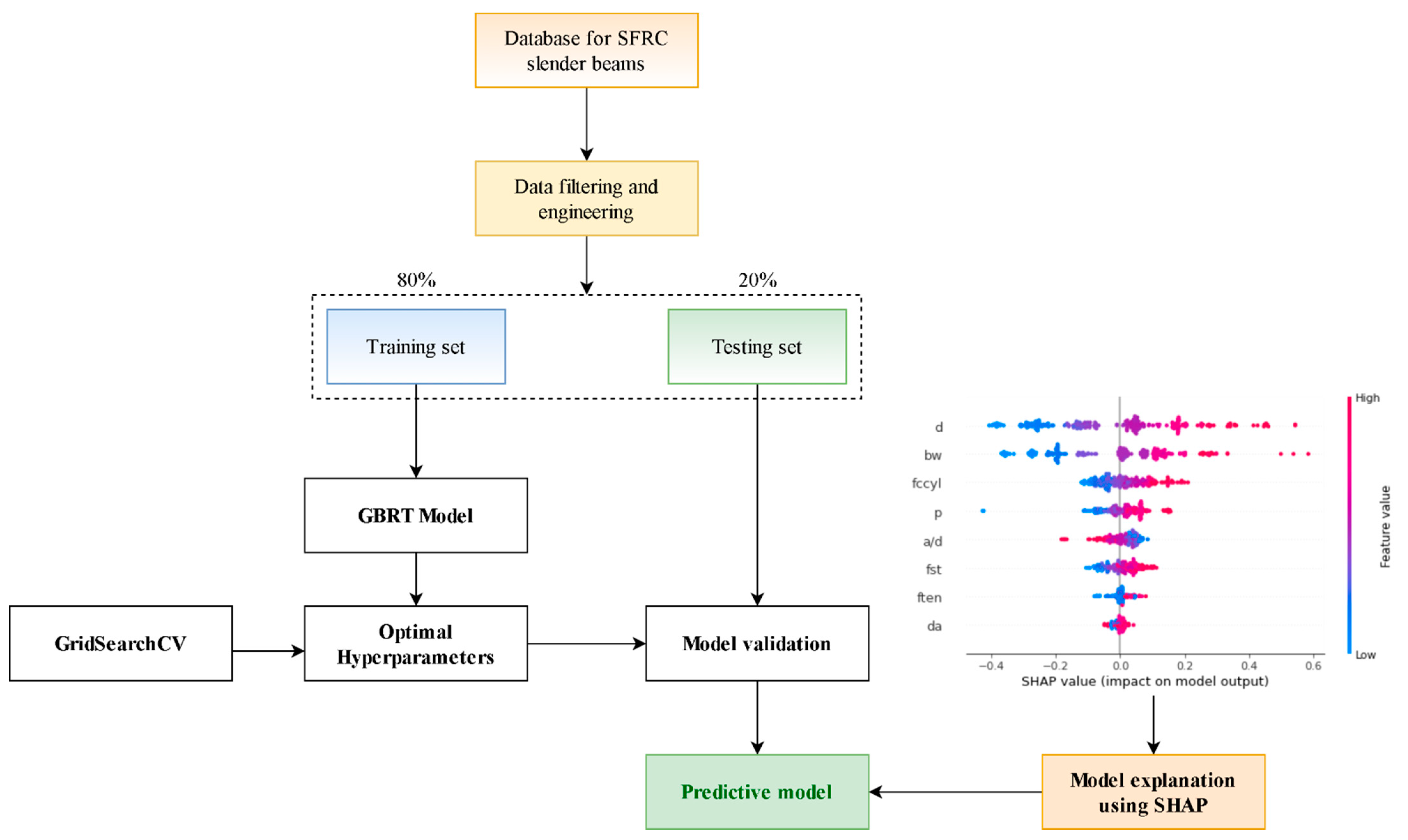
2.1. Research Methodology
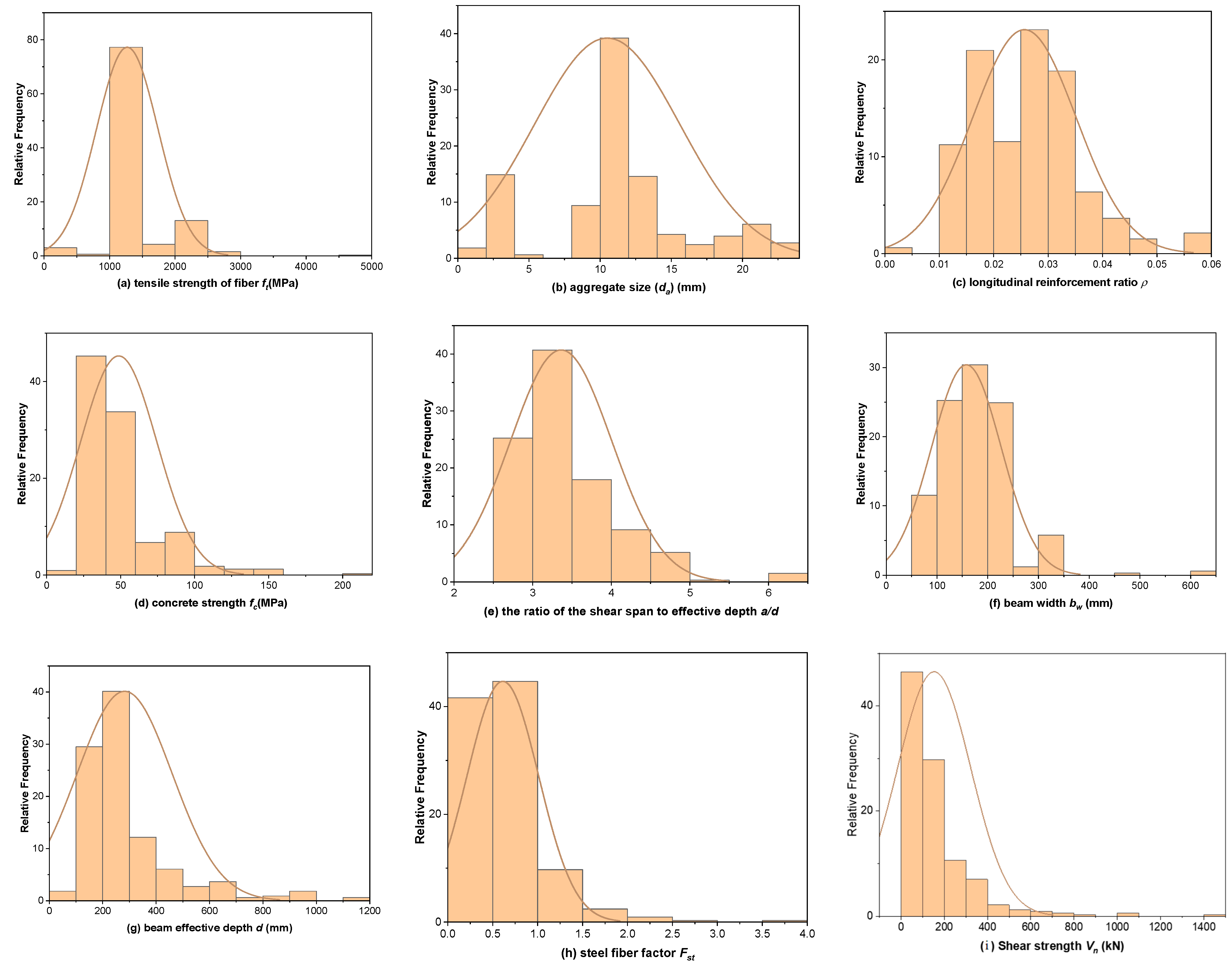
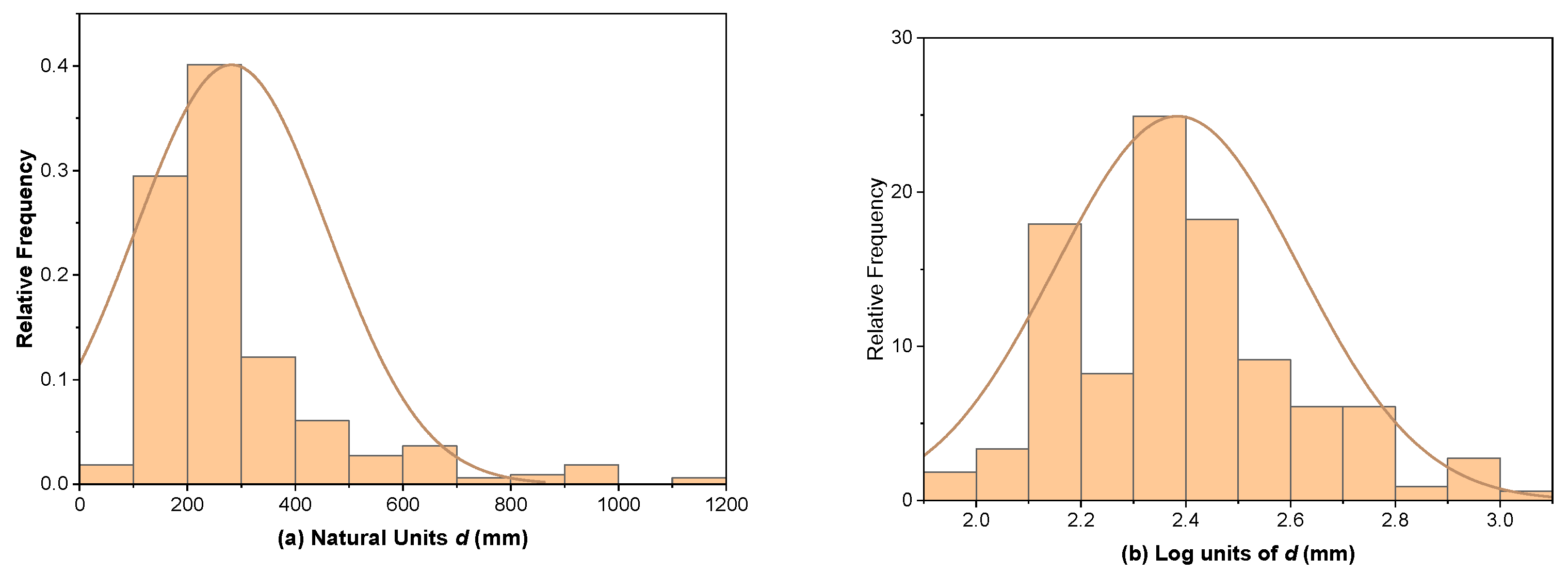
2.2. Dataset
2.3. Data-Splitting Procedure
2.4. GBRT Model Development
| Algorithm 1. The gradient boosting algorithm. |
| Input the iteration number D, loss function training set Initialize: F0 = For d = 1 to D do: end for Output: the final regression function Fd(x) |
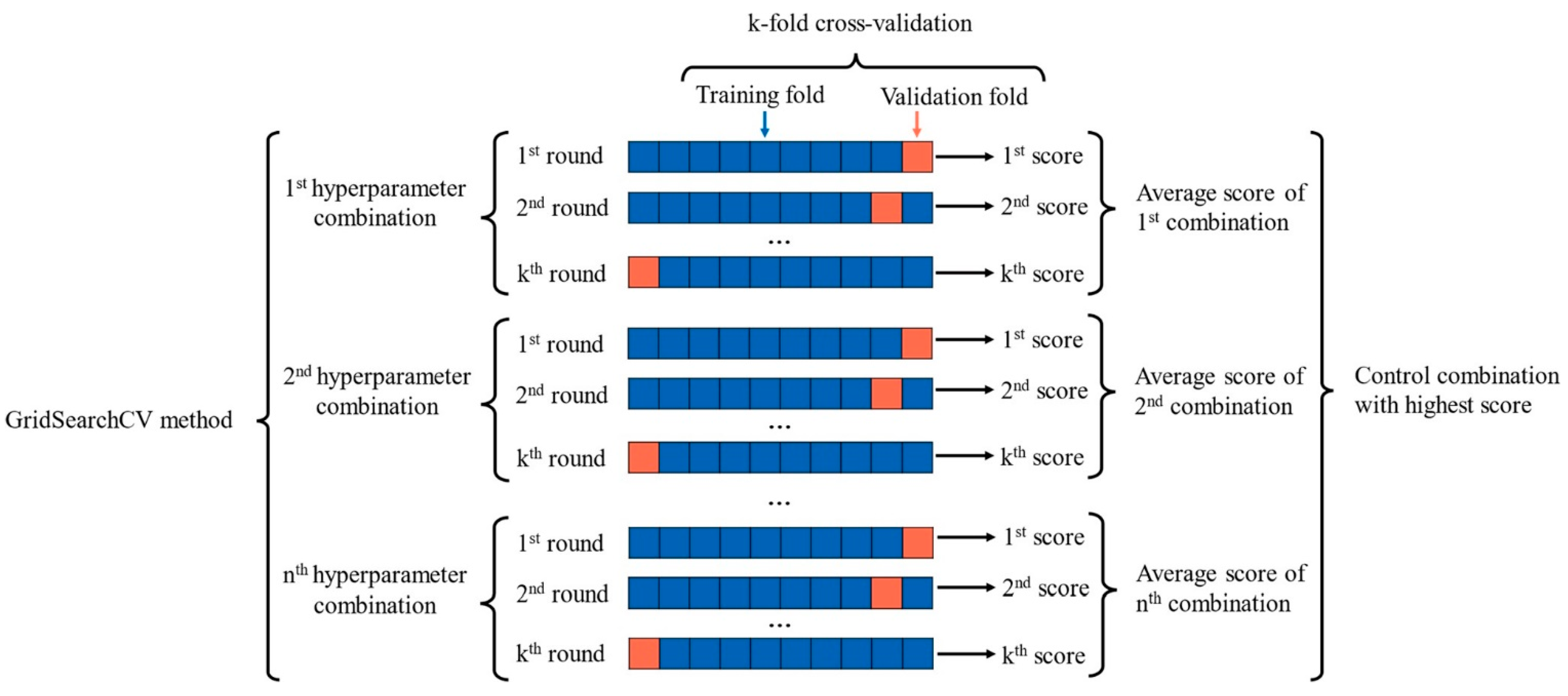
2.5. Cross-Validation
2.6. Hyperparameter Tuning
2.7. Performance Metrics
2.7.1. Model Performance Metrics
2.7.2. Model Uncertainty Metrics
2.8. Shapley Additive Explanations (SHAP) Framework
2.9. Programming Languages and Softwares
3. Model Results
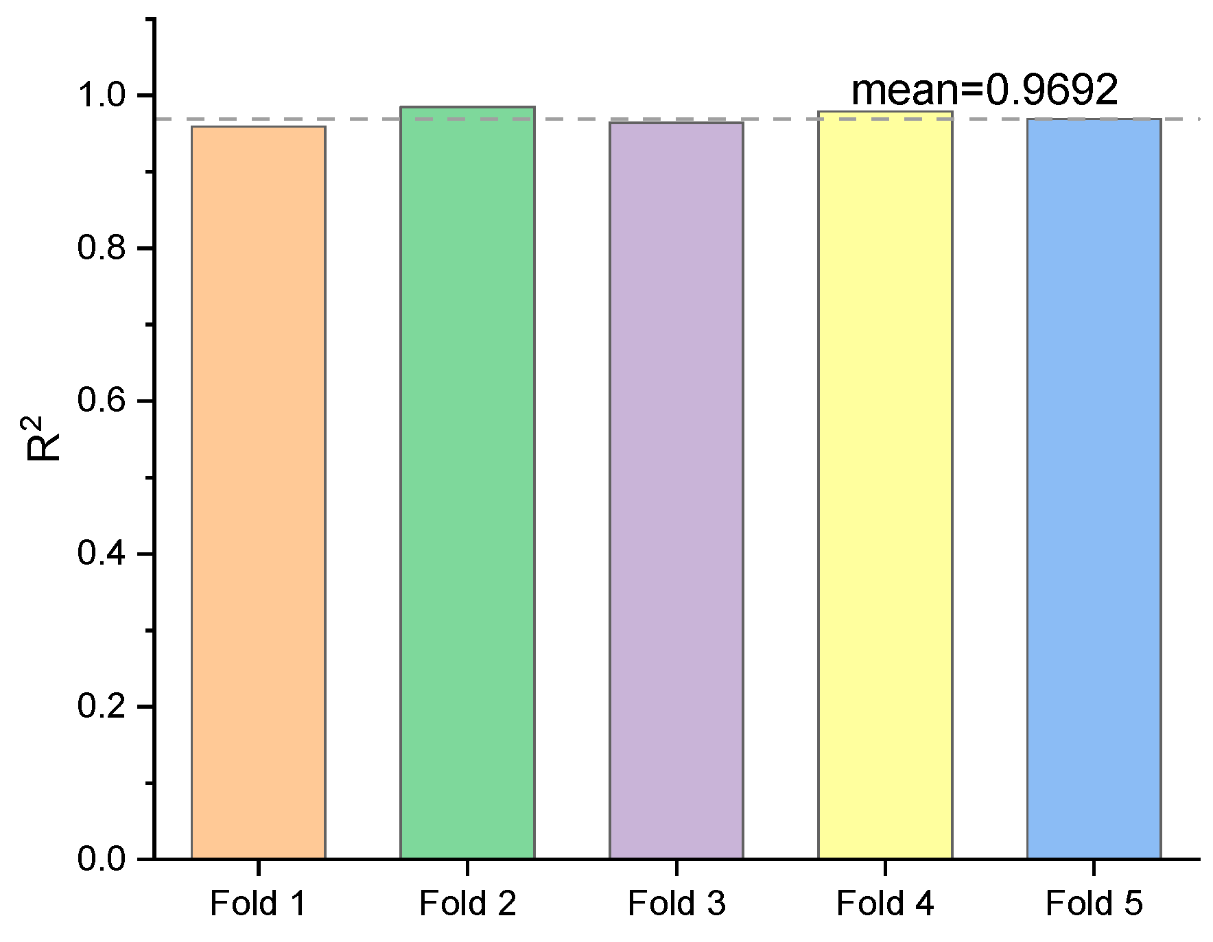
3.1. K-Fold Cross-Validation
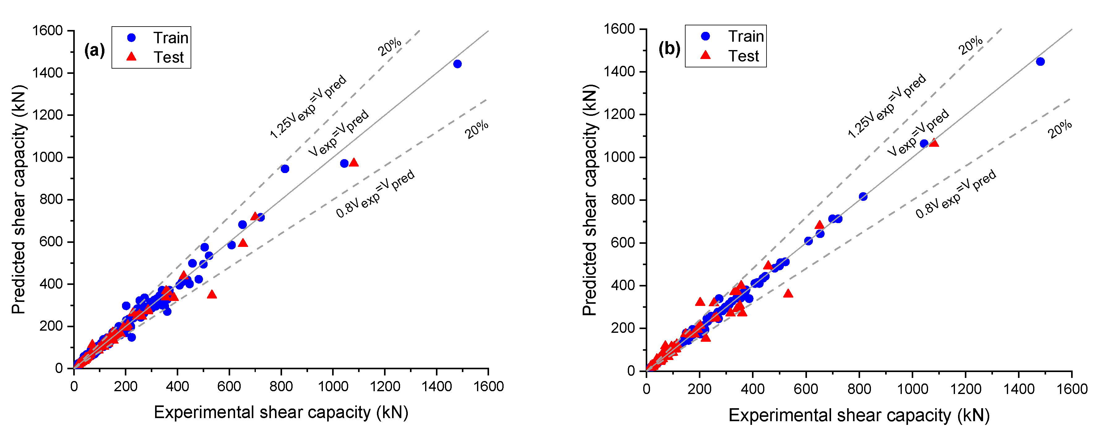
3.2. GBRT Performance on Testing Set
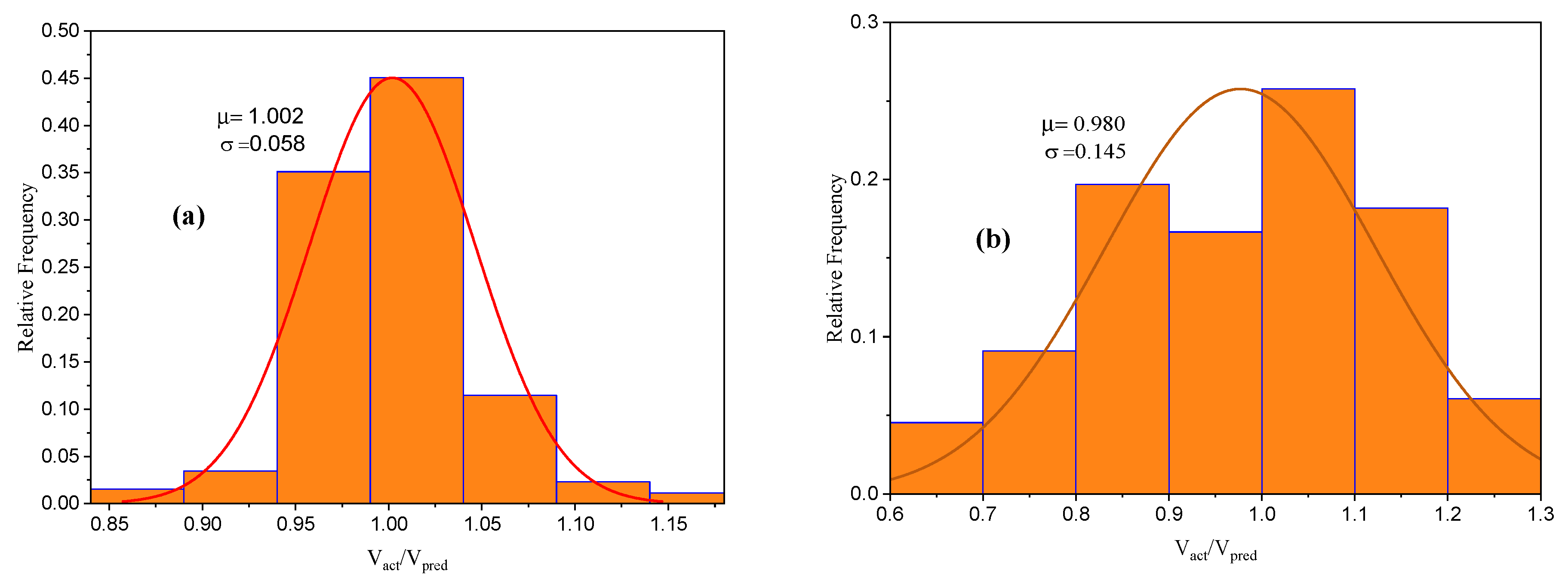
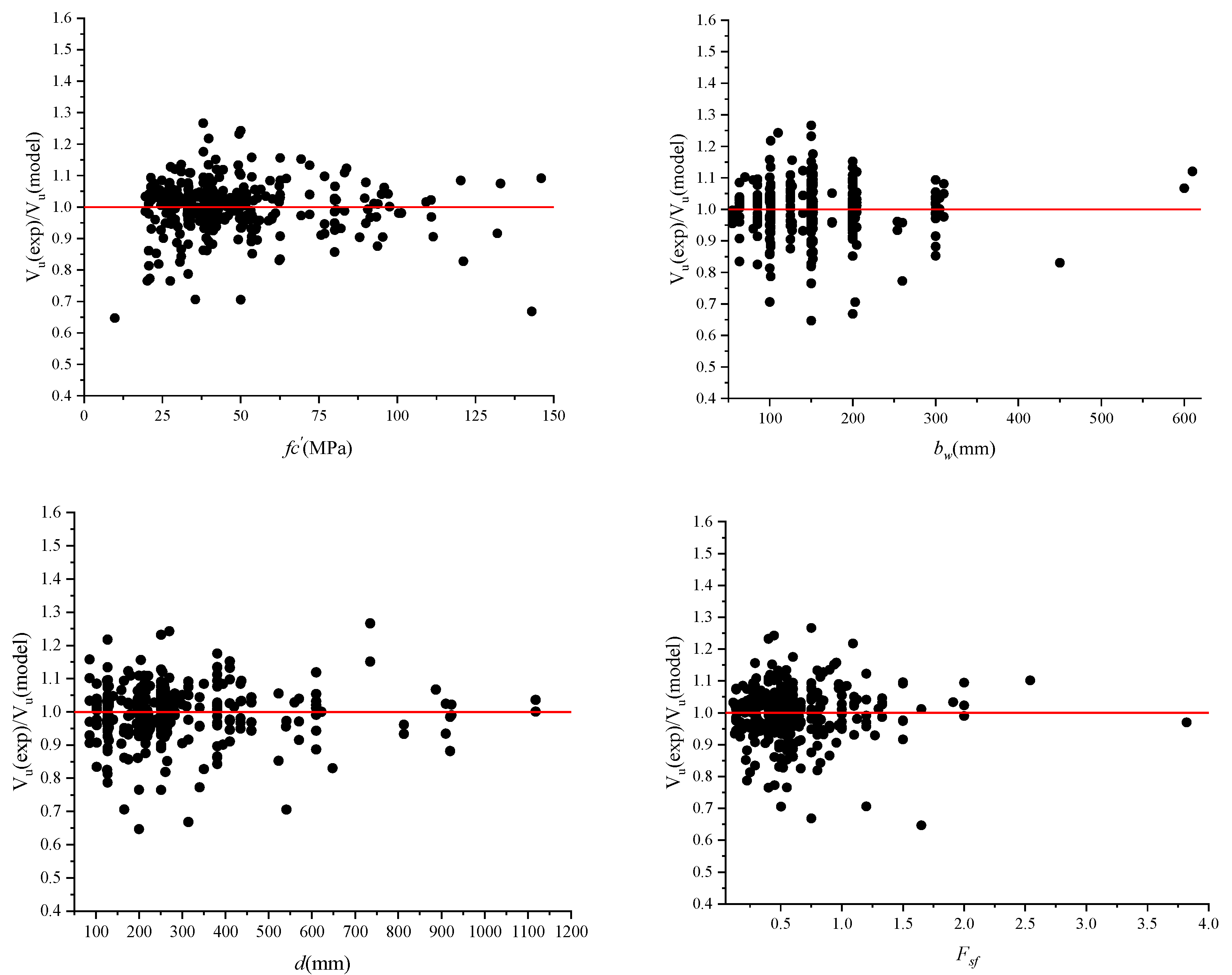
3.3. The Reliability of the GBRT Model Prediction
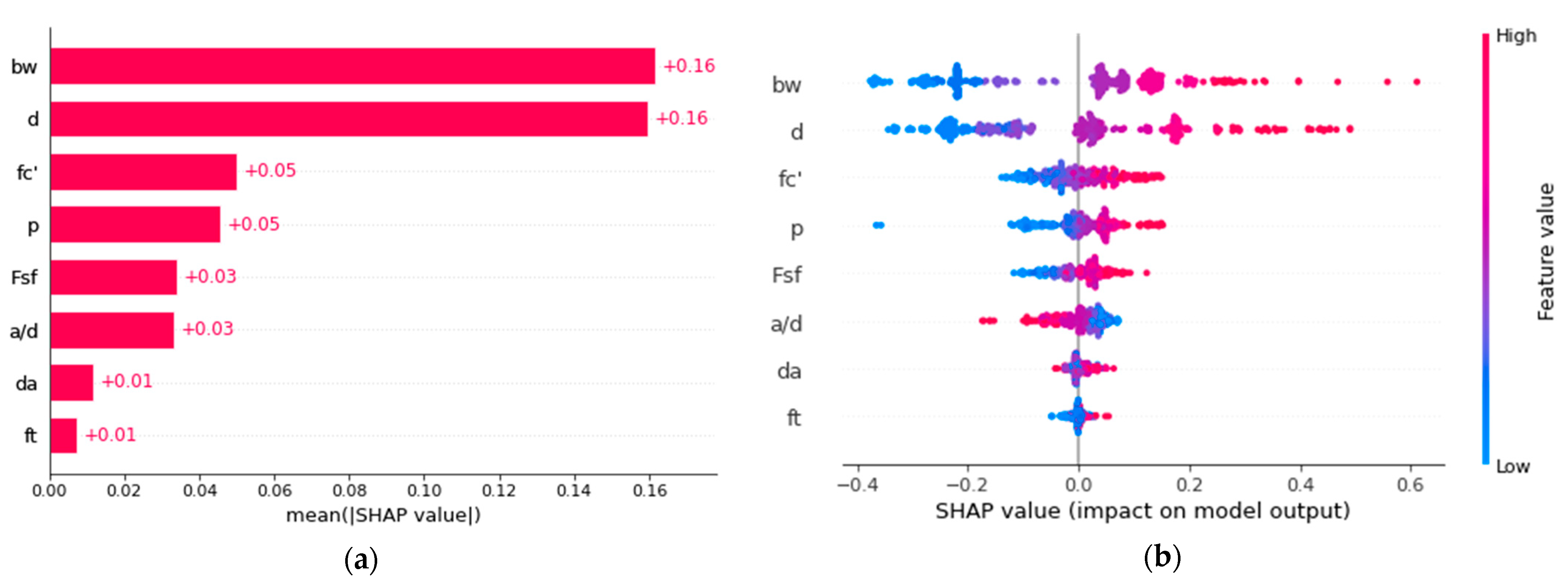
3.4. Interpretation of the GBRT Model
4. Conclusions
- The GBRT model predicts the shear capacity of SFRC slender beams with high accuracy. The model has R2 values of 0.963 and 0.972 for the testing and training sets, respectively. In addition, both the training and testing sets of the GBRT model have low RMSE and MAE values, indicating that the prediction capability of the GBRT model can be trusted with high confidence;
- A comparison between the predicted and experimental shear strengths was also performed, using previously established equations from the literature. The results show that the predicted values from previous models do not apply to a wide range of data and have a high variance;
- Most of the proposed equations from the literature show a mean value for the model uncertainty larger than 1, implying that they all underestimate the shear capacity of the SFRC slender beams from the database;
- With low error measurements and near unity, the results showed that the GBRT method surpassed the other models mentioned in this study.
Author Contributions
Funding
Institutional Review Board Statement
Informed Consent Statement
Data Availability Statement
Conflicts of Interest
Appendix A

| S.No | bw (mm) | d (mm) | ρ | a/d | da (mm) | fc (MPa) | ft (MPa) | Fst | Vu (kN) |
|---|---|---|---|---|---|---|---|---|---|
| 1 | 150 | 251 | 0.0267 | 3.49 | 12.5 | 28.1 | 1100 | 0.49 | 113 |
| 2 | 150 | 251 | 0.0267 | 3.49 | 12.5 | 25.3 | 1100 | 0.49 | 79 |
| 3 | 150 | 251 | 0.0267 | 3.49 | 12.5 | 27.9 | 1100 | 0.65 | 109 |
| 4 | 150 | 251 | 0.0267 | 3.49 | 12.5 | 26.2 | 1100 | 0.65 | 123 |
| 5 | 150 | 251 | 0.0267 | 3.49 | 12.5 | 28.1 | 1100 | 0.98 | 111 |
| 6 | 150 | 251 | 0.0267 | 3.49 | 12.5 | 27.3 | 1100 | 0.98 | 131 |
| 7 | 150 | 251 | 0.0267 | 3.49 | 12.5 | 27.5 | 1050 | 0.40 | 65 |
| 8 | 150 | 251 | 0.0267 | 3.49 | 12.5 | 24.9 | 1050 | 0.40 | 77 |
| 9 | 150 | 251 | 0.0267 | 3.49 | 12.5 | 27.8 | 1050 | 0.60 | 91 |
| 10 | 150 | 251 | 0.0267 | 3.49 | 12.5 | 27.3 | 1050 | 0.60 | 102 |
| 11 | 150 | 251 | 0.0267 | 3.49 | 12.5 | 26.3 | 1050 | 0.80 | 116 |
| 12 | 150 | 251 | 0.0267 | 3.49 | 12.5 | 27.1 | 1050 | 0.80 | 105 |
| 13 | 150 | 251 | 0.0267 | 3.49 | 12.5 | 53.4 | 1100 | 0.49 | 113 |
| 14 | 150 | 251 | 0.0267 | 3.49 | 12.5 | 54.1 | 1100 | 0.49 | 126 |
| 15 | 150 | 251 | 0.0267 | 3.49 | 12.5 | 53.2 | 1100 | 0.65 | 144 |
| 16 | 150 | 251 | 0.0267 | 3.49 | 12.5 | 55.3 | 1100 | 0.65 | 166 |
| 17 | 150 | 251 | 0.0267 | 3.49 | 12.5 | 64.6 | 1100 | 0.98 | 195 |
| 18 | 150 | 251 | 0.0267 | 3.49 | 12.5 | 59.9 | 1100 | 0.98 | 160 |
| 19 | 150 | 251 | 0.0267 | 3.49 | 12.5 | 47.8 | 1050 | 0.40 | 128 |
| 20 | 150 | 251 | 0.0267 | 3.49 | 12.5 | 49.5 | 1050 | 0.40 | 152 |
| 21 | 150 | 251 | 0.0267 | 3.49 | 12.5 | 55.3 | 1050 | 0.60 | 146 |
| 22 | 150 | 251 | 0.0267 | 3.49 | 12.5 | 56.4 | 1050 | 0.60 | 178 |
| 23 | 150 | 251 | 0.0267 | 3.49 | 12.5 | 53.4 | 1050 | 0.80 | 128 |
| 24 | 150 | 251 | 0.0267 | 3.49 | 12.5 | 51.0 | 1050 | 0.80 | 157 |
| 25 | 150 | 251 | 0.0267 | 3.49 | 12.5 | 27.8 | 1025 | 0.38 | 79 |
| 26 | 150 | 251 | 0.0267 | 3.49 | 12.5 | 27.2 | 1025 | 0.38 | 78 |
| 27 | 150 | 251 | 0.0267 | 3.49 | 12.5 | 27.6 | 1050 | 0.64 | 99 |
| 28 | 150 | 251 | 0.0267 | 3.49 | 12.5 | 27.9 | 1050 | 0.64 | 81 |
| 29 | 150 | 251 | 0.0267 | 3.49 | 12.5 | 34.7 | 1025 | 0.38 | 99 |
| 30 | 150 | 251 | 0.0267 | 3.49 | 12.5 | 36.2 | 1025 | 0.38 | 100 |
| 31 | 150 | 251 | 0.0267 | 3.49 | 12.5 | 37.0 | 1050 | 0.64 | 110 |
| 32 | 150 | 251 | 0.0267 | 3.49 | 12.5 | 38.3 | 1050 | 0.64 | 104 |
| 33 | 150 | 261 | 0.0195 | 3.45 | 20.0 | 32.9 | 1100 | 0.60 | 108 |
| 34 | 150 | 261 | 0.0195 | 3.45 | 20.0 | 23.8 | 1100 | 0.80 | 93 |
| 35 | 150 | 261 | 0.0195 | 3.45 | 20.0 | 24.1 | 1100 | 1.00 | 114 |
| 36 | 140 | 175 | 0.0128 | 2.50 | 12.0 | 82.0 | 1100 | 0.40 | 63 |
| 37 | 140 | 175 | 0.0128 | 2.50 | 12.0 | 83.2 | 1100 | 0.80 | 79 |
| 38 | 140 | 175 | 0.0128 | 2.50 | 12.0 | 83.8 | 1100 | 1.20 | 135 |
| 39 | 150 | 200 | 0.0134 | 2.50 | 22.0 | 33.7 | 1100 | 0.55 | 65 |
| 40 | 150 | 200 | 0.0134 | 2.50 | 22.0 | 24.5 | 1100 | 0.55 | 44 |
| 41 | 150 | 200 | 0.0134 | 2.50 | 22.0 | 21.4 | 1100 | 1.09 | 50 |
| 42 | 150 | 200 | 0.0134 | 2.50 | 12.0 | 9.8 | 1100 | 1.64 | 39 |
| 43 | 150 | 200 | 0.0134 | 3.50 | 22.0 | 20.2 | 1100 | 0.55 | 33 |
| 44 | 150 | 200 | 0.0134 | 3.50 | 22.0 | 21.4 | 1100 | 1.09 | 43 |
| 45 | 150 | 200 | 0.0134 | 3.50 | 12.0 | 27.9 | 1100 | 1.64 | 59 |
| 46 | 150 | 200 | 0.0134 | 4.50 | 22.0 | 24.5 | 1100 | 0.55 | 43 |
| 47 | 152 | 381 | 0.0271 | 3.40 | 10.0 | 49.2 | 1100 | 0.80 | 172 |
| 48 | 152 | 381 | 0.0271 | 3.40 | 10.0 | 31.0 | 1100 | 0.90 | 148 |
| 49 | 152 | 381 | 0.0271 | 3.40 | 10.0 | 44.9 | 1100 | 0.90 | 189 |
| 50 | 152 | 381 | 0.0271 | 3.40 | 10.0 | 44.9 | 1100 | 0.90 | 190 |
| 51 | 152 | 381 | 0.0271 | 3.40 | 10.0 | 49.2 | 1100 | 0.80 | 218 |
| 52 | 152 | 381 | 0.0271 | 3.40 | 10.0 | 31.0 | 1100 | 0.90 | 195 |
| 53 | 152 | 381 | 0.0271 | 3.50 | 10.0 | 38.1 | 1100 | 0.60 | 147 |
| 54 | 152 | 381 | 0.0271 | 3.50 | 10.0 | 38.1 | 1100 | 0.60 | 200 |
| 55 | 152 | 381 | 0.0197 | 3.50 | 10.0 | 38.1 | 1100 | 0.60 | 175 |
| 56 | 152 | 381 | 0.0197 | 3.50 | 10.0 | 38.1 | 1100 | 0.60 | 179 |
| 57 | 200 | 260 | 0.0181 | 2.50 | 10.0 | 40.0 | 1100 | 0.17 | 108 |
| 58 | 200 | 260 | 0.0181 | 2.50 | 10.0 | 38.7 | 1100 | 0.51 | 144 |
| 59 | 200 | 260 | 0.0115 | 2.50 | 10.0 | 40.0 | 1100 | 0.17 | 82 |
| 60 | 200 | 260 | 0.0115 | 2.50 | 10.0 | 38.7 | 1100 | 0.51 | 107 |
| 61 | 200 | 460 | 0.0280 | 3.40 | 10.0 | 37.7 | 1100 | 0.34 | 244 |
| 62 | 200 | 460 | 0.0280 | 3.40 | 10.0 | 38.8 | 1100 | 0.34 | 252 |
| 63 | 200 | 460 | 0.0280 | 3.40 | 10.0 | 37.7 | 1100 | 0.34 | 259 |
| 64 | 200 | 460 | 0.0280 | 3.40 | 10.0 | 37.7 | 1100 | 0.34 | 263 |
| 65 | 200 | 260 | 0.0356 | 3.50 | 10.0 | 46.9 | 1100 | 0.17 | 110 |
| 66 | 200 | 260 | 0.0356 | 3.50 | 10.0 | 43.7 | 1100 | 0.34 | 120 |
| 67 | 200 | 260 | 0.0356 | 3.50 | 10.0 | 48.3 | 1100 | 0.51 | 155 |
| 68 | 200 | 260 | 0.0283 | 3.50 | 10.0 | 37.7 | 1100 | 0.34 | 111 |
| 69 | 200 | 260 | 0.0283 | 3.50 | 10.0 | 38.8 | 1100 | 0.34 | 132 |
| 70 | 200 | 540 | 0.0273 | 3.50 | 10.0 | 37.7 | 1100 | 0.17 | 153 |
| 71 | 200 | 560 | 0.0273 | 3.50 | 10.0 | 38.8 | 1100 | 0.34 | 230 |
| 72 | 200 | 260 | 0.0181 | 4.00 | 10.0 | 41.2 | 1100 | 0.17 | 82 |
| 73 | 200 | 260 | 0.0181 | 4.00 | 10.0 | 40.3 | 1100 | 0.51 | 117 |
| 74 | 150 | 217 | 0.0185 | 2.95 | 10.0 | 35.0 | 1100 | 0.60 | 84 |
| 75 | 300 | 622 | 0.0198 | 2.81 | 10.0 | 34.0 | 2300 | 0.21 | 274 |
| 76 | 300 | 622 | 0.0198 | 2.81 | 10.0 | 36.0 | 2300 | 0.45 | 344 |
| 77 | 85 | 130 | 0.0205 | 2.52 | 9.6 | 51.9 | 2000 | 0.19 | 30 |
| 78 | 85 | 130 | 0.0205 | 3.02 | 9.6 | 51.9 | 2000 | 0.19 | 31 |
| 79 | 85 | 130 | 0.0205 | 2.52 | 9.6 | 33.3 | 2000 | 0.19 | 23 |
| 80 | 85 | 130 | 0.0205 | 3.02 | 9.6 | 33.3 | 2000 | 0.19 | 21 |
| 81 | 85 | 130 | 0.0205 | 3.02 | 9.6 | 51.7 | 2000 | 0.50 | 36 |
| 82 | 85 | 130 | 0.0205 | 3.02 | 9.6 | 30.6 | 2000 | 0.50 | 22 |
| 83 | 85 | 130 | 0.0205 | 3.02 | 9.6 | 31.0 | 2000 | 0.75 | 33 |
| 84 | 85 | 130 | 0.0205 | 2.52 | 9.6 | 51.7 | 2000 | 0.50 | 41 |
| 85 | 85 | 130 | 0.0205 | 3.52 | 9.6 | 41.7 | 2000 | 0.50 | 29 |
| 86 | 85 | 130 | 0.0205 | 2.52 | 9.6 | 48.7 | 2000 | 1.00 | 49 |
| 87 | 85 | 130 | 0.0205 | 3.52 | 9.6 | 48.8 | 2000 | 1.00 | 33 |
| 88 | 85 | 128 | 0.0370 | 3.06 | 9.6 | 41.7 | 2000 | 0.50 | 32 |
| 89 | 85 | 126 | 0.0572 | 3.11 | 9.6 | 41.7 | 2000 | 0.50 | 38 |
| 90 | 85 | 128 | 0.0370 | 3.06 | 9.6 | 30.6 | 2000 | 0.50 | 24 |
| 91 | 85 | 126 | 0.0572 | 3.11 | 9.6 | 30.6 | 2000 | 0.50 | 25 |
| 92 | 85 | 128 | 0.0370 | 3.06 | 9.6 | 48.8 | 2000 | 1.00 | 48 |
| 93 | 85 | 126 | 0.0572 | 3.11 | 9.6 | 48.8 | 2000 | 1.00 | 54 |
| 94 | 85 | 126 | 0.0572 | 3.11 | 9.6 | 53.6 | 2000 | 1.13 | 52 |
| 95 | 85 | 126 | 0.0572 | 3.11 | 9.6 | 43.2 | 2000 | 1.50 | 53 |
| 96 | 85 | 128 | 0.0370 | 3.06 | 9.6 | 53.6 | 2000 | 1.13 | 49 |
| 97 | 150 | 219 | 0.0191 | 2.80 | 10.0 | 40.9 | 1115 | 0.60 | 96 |
| 98 | 150 | 219 | 0.0191 | 2.80 | 10.0 | 40.9 | 1115 | 1.20 | 103 |
| 99 | 125 | 212 | 0.0152 | 3.00 | 19.0 | 30.8 | 1079 | 0.31 | 68 |
| 100 | 100 | 130 | 0.0309 | 3.08 | 10.0 | 38.7 | 1303 | 0.30 | 58 |
| 101 | 100 | 130 | 0.0309 | 3.08 | 10.0 | 42.4 | 1303 | 0.60 | 74 |
| 102 | 152 | 381 | 0.0196 | 3.44 | 10.0 | 44.8 | 1100 | 0.41 | 171 |
| 103 | 152 | 381 | 0.0196 | 3.44 | 10.0 | 44.8 | 1100 | 0.41 | 160 |
| 104 | 152 | 381 | 0.0196 | 3.44 | 10.0 | 38.1 | 1100 | 0.55 | 169 |
| 105 | 152 | 381 | 0.0196 | 3.44 | 10.0 | 38.1 | 1100 | 0.55 | 172 |
| 106 | 152 | 381 | 0.0263 | 3.44 | 10.0 | 31.0 | 1100 | 0.83 | 148 |
| 107 | 152 | 381 | 0.0263 | 3.44 | 10.0 | 31.0 | 1100 | 0.83 | 196 |
| 108 | 152 | 381 | 0.0263 | 3.44 | 10.0 | 44.9 | 1100 | 0.83 | 191 |
| 109 | 152 | 381 | 0.0263 | 3.44 | 10.0 | 44.9 | 1100 | 0.83 | 189 |
| 110 | 152 | 381 | 0.0263 | 3.44 | 10.0 | 49.2 | 1100 | 0.80 | 172 |
| 111 | 152 | 381 | 0.0263 | 3.44 | 10.0 | 49.2 | 1100 | 0.80 | 218 |
| 112 | 152 | 381 | 0.0196 | 3.44 | 10.0 | 43.3 | 2300 | 0.60 | 193 |
| 113 | 152 | 381 | 0.0196 | 3.44 | 10.0 | 43.3 | 2300 | 0.60 | 189 |
| 114 | 205 | 610 | 0.0196 | 3.50 | 10.0 | 50.8 | 1100 | 0.41 | 363 |
| 115 | 205 | 610 | 0.0196 | 3.50 | 10.0 | 50.8 | 1100 | 0.41 | 335 |
| 116 | 205 | 610 | 0.0196 | 3.50 | 10.0 | 28.7 | 1100 | 0.60 | 349 |
| 117 | 205 | 610 | 0.0196 | 3.50 | 10.0 | 28.7 | 1100 | 0.60 | 341 |
| 118 | 205 | 610 | 0.0152 | 3.50 | 10.0 | 42.3 | 1100 | 0.41 | 345 |
| 119 | 205 | 610 | 0.0152 | 3.50 | 10.0 | 29.6 | 1100 | 0.60 | 265 |
| 120 | 205 | 610 | 0.0152 | 3.50 | 10.0 | 29.6 | 1100 | 0.60 | 222 |
| 121 | 205 | 610 | 0.0196 | 3.50 | 10.0 | 44.4 | 1100 | 0.83 | 432 |
| 122 | 205 | 610 | 0.0196 | 3.50 | 10.0 | 42.8 | 1100 | 1.20 | 418 |
| 123 | 150 | 340 | 0.0308 | 2.50 | 12.5 | 58.9 | 1150 | 0.65 | 260 |
| 124 | 150 | 340 | 0.0308 | 2.50 | 12.5 | 51.7 | 1150 | 1.30 | 291 |
| 125 | 150 | 735 | 0.0106 | 3.81 | 12.5 | 42.0 | 1200 | 0.94 | 352 |
| 126 | 150 | 735 | 0.0106 | 3.81 | 12.5 | 38.0 | 1200 | 0.75 | 352 |
| 127 | 125 | 225 | 0.0349 | 2.89 | 10.0 | 90.0 | 1200 | 0.75 | 157 |
| 128 | 150 | 202 | 0.0117 | 2.97 | 10.0 | 21.3 | 1100 | 0.28 | 48 |
| 129 | 150 | 202 | 0.0117 | 2.97 | 10.0 | 19.6 | 1100 | 0.55 | 57 |
| 130 | 300 | 437 | 0.0150 | 3.09 | 10.0 | 21.3 | 1100 | 0.28 | 154 |
| 131 | 300 | 437 | 0.0150 | 3.09 | 10.0 | 19.6 | 1100 | 0.55 | 198 |
| 132 | 200 | 435 | 0.0104 | 2.51 | 20.0 | 24.8 | 1100 | 0.19 | 129 |
| 133 | 200 | 435 | 0.0104 | 2.51 | 20.0 | 33.5 | 1100 | 0.19 | 115 |
| 134 | 200 | 435 | 0.0104 | 2.51 | 20.0 | 33.5 | 1333 | 0.33 | 137 |
| 135 | 200 | 435 | 0.0104 | 2.51 | 20.0 | 38.6 | 1100 | 0.19 | 136 |
| 136 | 200 | 455 | 0.0099 | 2.51 | 15.0 | 24.4 | 1100 | 0.13 | 154 |
| 137 | 200 | 910 | 0.0104 | 2.50 | 20.0 | 24.4 | 1100 | 0.13 | 247 |
| 138 | 200 | 910 | 0.0104 | 2.50 | 20.0 | 55.0 | 1100 | 0.13 | 328 |
| 139 | 125 | 210 | 0.0153 | 4.00 | 19.0 | 44.6 | 1100 | 0.31 | 35 |
| 140 | 125 | 225 | 0.0349 | 2.89 | 10.0 | 90.0 | 1200 | 0.75 | 138 |
| 141 | 125 | 225 | 0.0349 | 2.89 | 10.0 | 90.0 | 1200 | 0.75 | 138 |
| 142 | 152 | 221 | 0.0120 | 2.50 | 10.0 | 34.0 | 1130 | 0.30 | 58 |
| 143 | 152 | 221 | 0.0239 | 2.50 | 10.0 | 34.0 | 1130 | 0.60 | 83 |
| 144 | 152 | 221 | 0.0239 | 2.50 | 10.0 | 34.0 | 1130 | 0.30 | 64 |
| 145 | 152 | 221 | 0.0239 | 3.50 | 10.0 | 34.0 | 1130 | 0.30 | 49 |
| 146 | 150 | 197 | 0.0136 | 2.80 | 20.0 | 29.1 | 1260 | 0.30 | 53 |
| 147 | 150 | 197 | 0.0136 | 3.60 | 20.0 | 29.1 | 1260 | 0.30 | 45 |
| 148 | 150 | 197 | 0.0136 | 2.80 | 20.0 | 29.9 | 1260 | 0.45 | 60 |
| 149 | 150 | 197 | 0.0204 | 2.80 | 20.0 | 29.9 | 1260 | 0.45 | 65 |
| 150 | 150 | 197 | 0.0136 | 2.80 | 20.0 | 20.6 | 1260 | 0.45 | 45 |
| 151 | 150 | 197 | 0.0204 | 2.80 | 20.0 | 20.6 | 1260 | 0.45 | 60 |
| 152 | 150 | 197 | 0.0204 | 2.80 | 20.0 | 33.4 | 1260 | 0.45 | 86 |
| 153 | 152 | 254 | 0.0248 | 3.50 | 10.0 | 29.0 | 1096 | 0.50 | 120 |
| 154 | 610 | 254 | 0.0247 | 3.50 | 10.0 | 29.0 | 1096 | 0.50 | 478 |
| 155 | 152 | 394 | 0.0286 | 3.61 | 10.0 | 39.0 | 1096 | 0.50 | 161 |
| 156 | 152 | 394 | 0.0286 | 3.61 | 10.0 | 39.0 | 1096 | 0.50 | 194 |
| 157 | 203 | 541 | 0.0254 | 3.45 | 10.0 | 50.0 | 1096 | 0.50 | 267 |
| 158 | 203 | 541 | 0.0254 | 3.45 | 10.0 | 50.0 | 1096 | 0.50 | 380 |
| 159 | 254 | 813 | 0.0270 | 3.50 | 10.0 | 50.0 | 1096 | 0.50 | 683 |
| 160 | 254 | 813 | 0.0270 | 3.50 | 10.0 | 50.0 | 1096 | 0.50 | 704 |
| 161 | 305 | 1118 | 0.0255 | 3.50 | 10.0 | 50.0 | 1096 | 0.50 | 1045 |
| 162 | 305 | 1118 | 0.0255 | 3.50 | 10.0 | 50.0 | 1096 | 0.50 | 1008 |
| 163 | 200 | 180 | 0.0447 | 3.33 | 16.0 | 90.6 | 2600 | 0.20 | 299 |
| 164 | 200 | 180 | 0.0447 | 3.33 | 16.0 | 83.2 | 1850 | 0.36 | 295 |
| 165 | 200 | 180 | 0.0447 | 3.33 | 16.0 | 80.5 | 2200 | 0.43 | 252 |
| 166 | 200 | 180 | 0.0447 | 3.33 | 16.0 | 80.5 | 2200 | 0.64 | 262 |
| 167 | 200 | 195 | 0.0309 | 3.08 | 16.0 | 39.4 | 1850 | 0.36 | 189 |
| 168 | 200 | 235 | 0.0428 | 2.77 | 16.0 | 91.4 | 1100 | 0.50 | 310 |
| 169 | 200 | 235 | 0.0428 | 2.77 | 16.0 | 93.3 | 2600 | 0.20 | 363 |
| 170 | 200 | 235 | 0.0428 | 2.77 | 16.0 | 89.6 | 1850 | 0.36 | 407 |
| 171 | 200 | 410 | 0.0306 | 2.93 | 18.0 | 76.8 | 2600 | 0.20 | 289 |
| 172 | 200 | 410 | 0.0306 | 2.93 | 18.0 | 76.8 | 2600 | 0.20 | 336 |
| 173 | 200 | 410 | 0.0306 | 2.93 | 18.0 | 72.0 | 1850 | 0.36 | 367 |
| 174 | 200 | 410 | 0.0306 | 2.93 | 18.0 | 72.0 | 1850 | 0.36 | 327 |
| 175 | 200 | 410 | 0.0306 | 2.93 | 18.0 | 69.3 | 2200 | 0.43 | 264 |
| 176 | 200 | 410 | 0.0306 | 2.93 | 18.0 | 69.3 | 2200 | 0.43 | 312 |
| 177 | 200 | 410 | 0.0306 | 2.93 | 18.0 | 60.2 | 2200 | 0.64 | 339 |
| 178 | 200 | 410 | 0.0306 | 2.93 | 18.0 | 75.7 | 2200 | 0.64 | 292 |
| 179 | 300 | 570 | 0.0287 | 2.98 | 18.0 | 76.8 | 2600 | 0.20 | 445 |
| 180 | 300 | 570 | 0.0287 | 2.98 | 18.0 | 72.0 | 1850 | 0.36 | 596 |
| 181 | 300 | 570 | 0.0287 | 2.98 | 18.0 | 60.2 | 2200 | 0.64 | 509 |
| 182 | 200 | 314 | 0.0350 | 3.50 | 0.4 | 131.5 | 2000 | 0.75 | 251 |
| 183 | 200 | 314 | 0.0350 | 3.50 | 0.4 | 154.5 | 2000 | 0.75 | 318 |
| 184 | 200 | 314 | 0.0350 | 3.50 | 0.4 | 145.6 | 2000 | 0.75 | 357 |
| 185 | 200 | 314 | 0.0350 | 3.50 | 0.4 | 132.8 | 2000 | 0.38 | 266 |
| 186 | 200 | 314 | 0.0350 | 3.50 | 0.4 | 143.3 | 2000 | 0.38 | 199 |
| 187 | 200 | 314 | 0.0350 | 3.50 | 0.4 | 152.9 | 2000 | 0.38 | 308 |
| 188 | 125 | 215 | 0.0037 | 4.00 | 10.0 | 92.6 | 260 | 0.75 | 24 |
| 189 | 125 | 215 | 0.0037 | 6.00 | 10.0 | 93.7 | 260 | 0.75 | 15 |
| 190 | 125 | 215 | 0.0283 | 4.00 | 10.0 | 95.4 | 260 | 0.38 | 61 |
| 191 | 125 | 215 | 0.0283 | 6.00 | 10.0 | 95.8 | 260 | 0.38 | 52 |
| 192 | 125 | 215 | 0.0283 | 4.00 | 10.0 | 97.5 | 260 | 0.75 | 85 |
| 193 | 125 | 215 | 0.0283 | 6.00 | 10.0 | 100.5 | 260 | 0.75 | 53 |
| 194 | 125 | 215 | 0.0283 | 4.00 | 10.0 | 97.1 | 260 | 1.13 | 94 |
| 195 | 125 | 215 | 0.0283 | 6.00 | 10.0 | 101.3 | 260 | 1.13 | 53 |
| 196 | 125 | 215 | 0.0458 | 4.00 | 10.0 | 93.8 | 260 | 0.75 | 104 |
| 197 | 125 | 215 | 0.0458 | 6.00 | 10.0 | 95.0 | 260 | 0.75 | 79 |
| 198 | 140 | 340 | 0.0167 | 2.50 | 19.0 | 36.0 | 1100 | 0.60 | 154 |
| 199 | 150 | 350 | 0.0561 | 2.86 | 2.0 | 121.1 | 2000 | 0.52 | 340 |
| 200 | 150 | 350 | 0.0561 | 2.86 | 2.0 | 120.3 | 2000 | 1.04 | 531 |
| 201 | 260 | 340 | 0.0172 | 4.00 | 10.0 | 21.0 | 1336 | 0.45 | 114 |
| 202 | 260 | 340 | 0.0172 | 4.00 | 10.0 | 56.0 | 1336 | 0.45 | 204 |
| 203 | 64 | 102 | 0.0220 | 3.00 | 2.4 | 53.0 | 1000 | 0.21 | 17 |
| 204 | 127 | 204 | 0.0221 | 3.00 | 2.4 | 53.0 | 1000 | 0.21 | 51 |
| 205 | 64 | 102 | 0.0220 | 3.00 | 2.4 | 50.2 | 1000 | 0.43 | 21 |
| 206 | 127 | 204 | 0.0221 | 3.00 | 2.4 | 50.2 | 1000 | 0.43 | 66 |
| 207 | 64 | 102 | 0.0220 | 3.00 | 2.4 | 62.6 | 1000 | 0.21 | 18 |
| 208 | 127 | 204 | 0.0221 | 3.00 | 2.4 | 62.6 | 1000 | 0.21 | 61 |
| 209 | 64 | 102 | 0.0220 | 2.50 | 2.4 | 62.6 | 1000 | 0.21 | 21 |
| 210 | 64 | 102 | 0.0220 | 2.75 | 2.4 | 62.6 | 1000 | 0.21 | 18 |
| 211 | 64 | 102 | 0.0110 | 3.00 | 2.4 | 62.6 | 1000 | 0.21 | 13 |
| 212 | 64 | 102 | 0.0330 | 3.00 | 2.4 | 62.6 | 1000 | 0.21 | 18 |
| 213 | 64 | 102 | 0.0330 | 3.00 | 2.4 | 54.1 | 1000 | 0.43 | 25 |
| 214 | 127 | 204 | 0.0221 | 3.00 | 9.0 | 22.7 | 1172 | 0.60 | 79 |
| 215 | 64 | 102 | 0.0220 | 3.00 | 9.0 | 22.7 | 1172 | 0.60 | 20 |
| 216 | 64 | 102 | 0.0110 | 3.00 | 9.0 | 22.7 | 1172 | 0.60 | 16 |
| 217 | 127 | 204 | 0.0221 | 3.00 | 9.0 | 26.0 | 1172 | 1.00 | 79 |
| 218 | 64 | 102 | 0.0220 | 3.00 | 9.0 | 26.0 | 1172 | 1.00 | 23 |
| 219 | 55 | 265 | 0.0431 | 3.43 | 14.0 | 41.9 | 1570 | 0.75 | 59 |
| 220 | 55 | 265 | 0.0431 | 4.91 | 14.0 | 36.9 | 1570 | 0.75 | 43 |
| 221 | 55 | 265 | 0.0276 | 3.43 | 14.0 | 33.9 | 1570 | 0.75 | 46 |
| 222 | 200 | 265 | 0.0178 | 3.02 | 10.0 | 47.9 | 1100 | 0.25 | 91 |
| 223 | 200 | 265 | 0.0178 | 3.02 | 10.0 | 38.0 | 1100 | 0.38 | 106 |
| 224 | 200 | 265 | 0.0178 | 3.02 | 10.0 | 42.2 | 1100 | 0.50 | 149 |
| 225 | 200 | 265 | 0.0178 | 3.02 | 10.0 | 45.4 | 1100 | 0.13 | 115 |
| 226 | 200 | 265 | 0.0178 | 3.02 | 10.0 | 44.4 | 1100 | 0.19 | 144 |
| 227 | 200 | 265 | 0.0178 | 3.02 | 10.0 | 40.3 | 1100 | 0.25 | 147 |
| 228 | 200 | 265 | 0.0178 | 3.02 | 10.0 | 53.7 | 1100 | 0.11 | 107 |
| 229 | 200 | 265 | 0.0178 | 3.02 | 10.0 | 46.0 | 1100 | 0.16 | 123 |
| 230 | 200 | 265 | 0.0178 | 3.02 | 10.0 | 42.2 | 1100 | 0.21 | 151 |
| 231 | 200 | 310 | 0.0113 | 2.55 | 9.5 | 39.8 | 1100 | 0.30 | 131 |
| 232 | 200 | 285 | 0.0333 | 2.77 | 9.5 | 39.8 | 1100 | 0.30 | 220 |
| 233 | 200 | 260 | 0.0355 | 3.46 | 14.0 | 46.4 | 1100 | 0.16 | 110 |
| 234 | 200 | 260 | 0.0355 | 3.46 | 14.0 | 43.2 | 1100 | 0.33 | 120 |
| 235 | 200 | 260 | 0.0355 | 3.46 | 14.0 | 47.6 | 1100 | 0.49 | 155 |
| 236 | 200 | 260 | 0.0181 | 2.50 | 14.0 | 39.1 | 1100 | 0.16 | 108 |
| 237 | 200 | 260 | 0.0181 | 2.50 | 14.0 | 38.6 | 1100 | 0.49 | 144 |
| 238 | 200 | 260 | 0.0181 | 4.04 | 14.0 | 40.7 | 1100 | 0.16 | 83 |
| 239 | 200 | 260 | 0.0181 | 4.04 | 14.0 | 42.4 | 1100 | 0.49 | 117 |
| 240 | 200 | 260 | 0.0181 | 2.50 | 14.0 | 26.5 | 1100 | 0.11 | 100 |
| 241 | 200 | 260 | 0.0181 | 2.50 | 14.0 | 27.2 | 1100 | 0.34 | 120 |
| 242 | 200 | 260 | 0.0181 | 2.50 | 14.0 | 46.8 | 1100 | 0.33 | 158 |
| 243 | 175 | 210 | 0.0401 | 4.50 | 10.0 | 36.4 | 1050 | 0.30 | 80 |
| 244 | 175 | 210 | 0.0401 | 4.50 | 10.0 | 38.4 | 1050 | 0.60 | 114 |
| 245 | 175 | 210 | 0.0401 | 4.50 | 10.0 | 40.8 | 1050 | 0.90 | 115 |
| 246 | 175 | 210 | 0.0401 | 4.50 | 10.0 | 38.5 | 1050 | 0.60 | 69 |
| 247 | 101 | 127 | 0.0309 | 4.40 | 2.0 | 33.2 | 1100 | 0.11 | 32 |
| 248 | 101 | 127 | 0.0309 | 4.20 | 2.0 | 33.2 | 1100 | 0.11 | 31 |
| 249 | 101 | 127 | 0.0309 | 4.20 | 2.0 | 33.2 | 1100 | 0.11 | 28 |
| 250 | 101 | 127 | 0.0309 | 4.20 | 2.0 | 33.2 | 1100 | 0.11 | 25 |
| 251 | 101 | 127 | 0.0309 | 4.30 | 2.0 | 33.2 | 1100 | 0.11 | 30 |
| 252 | 101 | 127 | 0.0309 | 4.30 | 2.0 | 33.2 | 1100 | 0.11 | 28 |
| 253 | 101 | 127 | 0.0309 | 4.00 | 2.0 | 40.2 | 1100 | 0.22 | 33 |
| 254 | 101 | 127 | 0.0309 | 4.00 | 2.0 | 40.2 | 1100 | 0.22 | 31 |
| 255 | 101 | 127 | 0.0309 | 4.00 | 2.0 | 40.2 | 1100 | 0.22 | 33 |
| 256 | 101 | 127 | 0.0309 | 4.40 | 2.0 | 33.2 | 1100 | 0.11 | 28 |
| 257 | 101 | 127 | 0.0309 | 4.40 | 2.0 | 33.2 | 1100 | 0.11 | 27 |
| 258 | 101 | 127 | 0.0309 | 4.00 | 2.0 | 33.2 | 1100 | 0.10 | 30 |
| 259 | 101 | 127 | 0.0309 | 4.00 | 2.0 | 33.2 | 1100 | 0.10 | 30 |
| 260 | 101 | 127 | 0.0309 | 4.00 | 2.0 | 33.2 | 1100 | 0.10 | 33 |
| 261 | 101 | 127 | 0.0309 | 4.60 | 2.0 | 33.2 | 1100 | 0.10 | 26 |
| 262 | 101 | 127 | 0.0309 | 4.40 | 2.0 | 33.2 | 1100 | 0.10 | 27 |
| 263 | 101 | 127 | 0.0309 | 4.40 | 2.0 | 33.2 | 1100 | 0.10 | 26 |
| 264 | 101 | 127 | 0.0309 | 5.00 | 2.0 | 33.2 | 1100 | 0.10 | 24 |
| 265 | 101 | 127 | 0.0309 | 4.80 | 2.0 | 33.2 | 1100 | 0.10 | 22 |
| 266 | 101 | 127 | 0.0309 | 4.00 | 2.0 | 40.2 | 1100 | 0.20 | 31 |
| 267 | 101 | 127 | 0.0309 | 4.20 | 2.0 | 40.2 | 1100 | 0.20 | 34 |
| 268 | 101 | 127 | 0.0309 | 4.20 | 2.0 | 40.2 | 1100 | 0.20 | 30 |
| 269 | 101 | 127 | 0.0309 | 4.20 | 2.0 | 40.2 | 1100 | 0.20 | 32 |
| 270 | 101 | 127 | 0.0309 | 3.20 | 2.0 | 39.7 | 1100 | 0.41 | 37 |
| 271 | 101 | 127 | 0.0309 | 3.40 | 2.0 | 39.7 | 1100 | 0.41 | 34 |
| 272 | 101 | 127 | 0.0309 | 3.40 | 2.0 | 39.7 | 1100 | 0.41 | 33 |
| 273 | 101 | 127 | 0.0309 | 3.40 | 2.0 | 39.7 | 1100 | 0.41 | 42 |
| 274 | 101 | 127 | 0.0309 | 3.40 | 2.0 | 39.7 | 1100 | 0.41 | 39 |
| 275 | 101 | 127 | 0.0309 | 4.80 | 2.0 | 33.2 | 1100 | 0.10 | 24 |
| 276 | 101 | 127 | 0.0309 | 4.80 | 2.0 | 33.2 | 1100 | 0.10 | 23 |
| 277 | 101 | 127 | 0.0309 | 4.80 | 2.0 | 33.2 | 1100 | 0.10 | 26 |
| 278 | 100 | 127 | 0.0199 | 3.60 | 2.0 | 20.7 | 4913 | 0.13 | 21 |
| 279 | 100 | 127 | 0.0199 | 3.60 | 2.0 | 20.7 | 2350 | 0.42 | 29 |
| 280 | 100 | 127 | 0.0199 | 4.80 | 2.0 | 20.7 | 2350 | 0.42 | 24 |
| 281 | 100 | 175 | 0.0359 | 3.00 | 13.0 | 80.0 | 1856 | 0.25 | 56 |
| 282 | 100 | 175 | 0.0359 | 3.00 | 13.0 | 80.0 | 1856 | 0.50 | 72 |
| 283 | 100 | 175 | 0.0359 | 4.50 | 13.0 | 80.0 | 1856 | 0.25 | 49 |
| 284 | 100 | 175 | 0.0359 | 4.50 | 13.0 | 80.0 | 1856 | 0.50 | 60 |
| 285 | 200 | 300 | 0.0308 | 2.50 | 10.0 | 110.0 | 2000 | 0.56 | 284 |
| 286 | 200 | 300 | 0.0308 | 3.50 | 10.0 | 111.5 | 2000 | 0.56 | 209 |
| 287 | 200 | 300 | 0.0308 | 4.50 | 10.0 | 110.8 | 2000 | 0.56 | 212 |
| 288 | 152 | 283 | 0.0199 | 2.50 | 9.5 | 33.1 | 1100 | 1.00 | 136 |
| 289 | 152.4 | 283 | 0.0199 | 2.50 | 9.5 | 33.2 | 1100 | 1.00 | 145 |
| 290 | 152 | 283 | 0.0199 | 2.50 | 9.5 | 33.0 | 1100 | 2.00 | 134 |
| 291 | 152 | 283 | 0.0199 | 2.50 | 9.5 | 34.4 | 1100 | 2.00 | 138 |
| 292 | 100 | 166 | 0.0343 | 3.02 | 10.0 | 39.4 | 1200 | 0.30 | 31 |
| 293 | 100 | 166 | 0.0343 | 3.02 | 10.0 | 39.2 | 1200 | 0.60 | 52 |
| 294 | 100 | 166 | 0.0343 | 3.02 | 10.0 | 40.0 | 1200 | 0.90 | 54 |
| 295 | 100 | 166 | 0.0343 | 3.02 | 10.0 | 35.5 | 1200 | 1.20 | 48 |
| 296 | 100 | 159 | 0.0478 | 3.14 | 10.0 | 58.0 | 1200 | 0.60 | 74 |
| 297 | 100 | 159 | 0.0478 | 3.14 | 10.0 | 80.1 | 1200 | 0.30 | 73 |
| 298 | 100 | 159 | 0.0478 | 3.14 | 10.0 | 88.0 | 1200 | 0.60 | 81 |
| 299 | 150 | 219 | 0.0191 | 2.80 | 10.0 | 80.0 | 1100 | 0.55 | 114 |
| 300 | 125 | 212 | 0.0152 | 3.77 | 10.0 | 59.4 | 1100 | 0.27 | 43 |
| 301 | 125 | 212 | 0.0152 | 3.77 | 10.0 | 49.6 | 1100 | 0.40 | 45 |
| 302 | 125 | 210 | 0.0228 | 3.81 | 10.0 | 49.7 | 1100 | 0.41 | 44 |
| 303 | 125 | 210 | 0.0228 | 3.81 | 10.0 | 51.5 | 1100 | 0.55 | 58 |
| 304 | 125 | 210 | 0.0228 | 3.81 | 12.0 | 54.5 | 1100 | 0.55 | 59 |
| 305 | 100 | 140 | 0.0112 | 2.50 | 12.5 | 36.1 | 1100 | 0.31 | 41 |
| 306 | 100 | 85 | 0.0166 | 3.52 | 10.0 | 54.8 | 1100 | 0.95 | 20 |
| 307 | 100 | 85 | 0.0166 | 3.52 | 10.0 | 49.3 | 1100 | 1.43 | 22 |
| 308 | 100 | 85 | 0.0166 | 3.52 | 10.0 | 49.3 | 1100 | 1.43 | 19 |
| 309 | 100 | 85 | 0.0166 | 3.52 | 10.0 | 53.7 | 1100 | 2.86 | 20 |
| 310 | 100 | 85 | 0.0166 | 3.52 | 10.0 | 53.5 | 1100 | 0.71 | 23 |
| 311 | 100 | 85 | 0.0166 | 3.52 | 10.0 | 53.5 | 1100 | 0.71 | 18 |
| 312 | 200 | 273 | 0.0348 | 2.75 | 22.0 | 110.9 | 1000 | 0.48 | 201 |
| 313 | 200 | 273 | 0.0348 | 2.75 | 22.0 | 109.2 | 1000 | 0.50 | 209 |
| 314 | 80 | 165 | 0.0171 | 2.99 | 4.0 | 41.2 | 800 | 0.50 | 33 |
| 315 | 80 | 165 | 0.0171 | 2.99 | 4.0 | 39.9 | 800 | 0.75 | 41 |
| 316 | 300 | 420 | 0.0322 | 3.21 | 20.0 | 62.3 | 1400 | 0.49 | 411 |
| 317 | 450 | 648 | 0.0327 | 3.26 | 20.0 | 62.3 | 1400 | 0.49 | 793 |
| 318 | 600 | 887 | 0.0343 | 3.26 | 20.0 | 62.3 | 1400 | 0.49 | 1430 |
| 319 | 70 | 270 | 0.0332 | 2.56 | 10.0 | 50.0 | 1100 | 0.33 | 81 |
| 320 | 110 | 270 | 0.0212 | 2.56 | 10.0 | 50.0 | 1100 | 0.33 | 96 |
| 321 | 150 | 270 | 0.0155 | 2.56 | 10.0 | 50.0 | 1100 | 0.33 | 109 |
| 322 | 310 | 258 | 0.0250 | 3.00 | 10.0 | 23.0 | 1100 | 0.55 | 210 |
| 323 | 310 | 240 | 0.0403 | 3.00 | 10.0 | 41.0 | 1100 | 0.55 | 280 |
| 324 | 300 | 531 | 0.0188 | 3.00 | 10.0 | 23.0 | 1100 | 0.55 | 248 |
| 325 | 300 | 523 | 0.0255 | 3.00 | 10.0 | 23.0 | 1100 | 0.55 | 238 |
| 326 | 300 | 523 | 0.0255 | 3.00 | 10.0 | 41.0 | 1100 | 0.55 | 440 |
| 327 | 300 | 923 | 0.0144 | 3.00 | 10.0 | 41.0 | 1100 | 0.55 | 479 |
| 328 | 300 | 920 | 0.0203 | 3.00 | 10.0 | 41.0 | 1100 | 0.55 | 484 |
| 329 | 300 | 923 | 0.0144 | 3.00 | 10.0 | 80.0 | 1100 | 0.55 | 633 |
| 330 | 300 | 920 | 0.0203 | 3.00 | 10.0 | 80.0 | 1100 | 0.55 | 631 |
References
- Khuntia, M.; Stojadinovic, B.; Goel, S.C. Shear strength of normal and high-strength fiber reinforced concrete beams without stirrups. Struct. J. 1999, 96, 282–289. [Google Scholar]
- Shahnewaz, M.; Alam, M.S. Genetic algorithm for predicting shear strength of steel fiber reinforced concrete beam with parameter identification and sensitivity analysis. J. Build. Eng. 2020, 29, 101205. [Google Scholar] [CrossRef]
- Dinh, H.H. Shear Behavior of Steel Fiber Reinforced Concrete Beams without Stirrup Reinforcement. Ph.D. Thesis, University of Michigan, Ann Arbor, MI, USA, 2009. [Google Scholar]
- Raju, R.A.; Akiyama, M.; Lim, S.; Kakegawa, T.; Hosono, Y. A novel casting procedure for SFRC piles without shear reinforcement using the centrifugal forming technique to manipulate the fiber orientation and distribution. Constr. Build. Mater. 2021, 303, 124232. [Google Scholar] [CrossRef]
- Yaseen, Z.M.; Tran, M.T.; Kim, S.; Bakhshpoori, T.; Deo, R.C. Shear strength prediction of steel fiber reinforced concrete beam using hybrid intelligence models: A new approach. Eng. Struct. 2018, 177, 244–255. [Google Scholar] [CrossRef]
- Kim, K.S.; Lee, D.H.; Hwang, J.-H.; Kuchma, D.A. Shear behavior model for steel fiber-reinforced concrete members without transverse reinforcements. Compos. Part B Eng. 2012, 43, 2324–2334. [Google Scholar] [CrossRef]
- Narayanan, R.; Darwish, I. Use of steel fibers as shear reinforcement. Struct. J. 1987, 84, 216–227. [Google Scholar]
- Gandomi, A.; Alavi, A.; Yun, G. Nonlinear modeling of shear strength of SFRC beams using linear genetic programming. Struct. Eng. Mech. 2011, 38, 1–25. [Google Scholar] [CrossRef]
- Özcan, D.M.; Bayraktar, A.; Şahin, A.; Haktanir, T.; Türker, T. Experimental and finite element analysis on the steel fiber-reinforced concrete (SFRC) beams ultimate behavior. Constr. Build. Mater. 2009, 23, 1064–1077. [Google Scholar] [CrossRef]
- Spinella, N.; Colajanni, P.; Recupero, A. Simple plastic model for shear critical SFRC beams. J. Struct. Eng. 2010, 136, 390–400. [Google Scholar] [CrossRef] [Green Version]
- Arslan, G. Shear strength of steel fiber reinforced concrete (SFRC) slender beams. KSCE J. Civ. Eng. 2014, 18, 587–594. [Google Scholar] [CrossRef]
- Hanai, J.B.; Holanda, K.M.A. Similarities between punching and shear strength of steel fiber reinforced concrete (SFRC) slabs and beams. IBRACON Struct. Mater. J. 2008, 1, 1–16. [Google Scholar]
- Lantsoght, E.O. Database of shear experiments on steel fiber reinforced concrete beams without stirrups. Materials 2019, 12, 917. [Google Scholar] [CrossRef] [PubMed] [Green Version]
- Lantsoght, E.O. How do steel fibers improve the shear capacity of reinforced concrete beams without stirrups? Compos. Part B Eng. 2019, 175, 107079. [Google Scholar]
- Marì Bernat, A.; Spinella, N.; Recupero, A.; Cladera, A. Mechanical model for the shear strength of steel fiber reinforced concrete (SFRC) beams without stirrups. Mater. Struct. 2020, 53, 28. [Google Scholar] [CrossRef]
- Keshtegar, B.; Bagheri, M.; Yaseen, Z.M. Shear strength of steel fiber-unconfined reinforced concrete beam simulation: Application of novel intelligent model. Compos. Struct. 2019, 212, 230–242. [Google Scholar] [CrossRef]
- Abambres, M.; Lantsoght, E.O. ANN-based shear capacity of steel fiber-reinforced concrete beams without stirrups. Fibers 2019, 7, 88. [Google Scholar] [CrossRef] [Green Version]
- El-Chabib, H.; Nehdi, M.; Said, A. Predicting shear capacity of NSC and HSC slender beams without stirrups using artificial intelligence. Comput. Concr. Int. J. 2005, 2, 79–96. [Google Scholar] [CrossRef]
- Nehdi, M.; El Chabib, H.; Said, A. Evaluation of shear capacity of FRP reinforced concrete beams using artificial neural networks. Smart Struct. Syst. 2006, 2, 81–100. [Google Scholar] [CrossRef]
- Chaabene, W.B.; Nehdi, M.L. Novel soft computing hybrid model for predicting shear strength and failure mode of SFRC beams with superior accuracy. Compos. Part C Open Access 2020, 3, 100070. [Google Scholar] [CrossRef]
- Greenough, T.; Nehdi, M. Shear behavior of fiber-reinforced self-consolidating concrete slender beams. ACI Mater. J. 2008, 105, 468. [Google Scholar]
- Kara, I.F. Empirical modeling of shear strength of steel fiber reinforced concrete beams by gene expression programming. Neural Comput. Appl. 2013, 23, 823–834. [Google Scholar] [CrossRef]
- Mukherjee, S.; Manju, S. An improved parametric formulation for the variationally correct distortion immune three-noded bar element. Struct. Eng. Mech. 2011, 38, 261. [Google Scholar] [CrossRef]
- Shahnewaz, M.; Tannert, M. Shear strength prediction of steel fiber reinforced concrete beams from genetic programming and its sensitivity analysis. In Proceedings of the FRC: The Modern Landscape BEFIB 2016 9th Rilem International Symposium on Fiber Reinforced Concrete, Vancouver, BC, Canada, 19–21 September 2016. [Google Scholar]
- Slater, E.; Moni, M.; Alam, M.S. Predicting the shear strength of steel fiber reinforced concrete beams. Constr. Build. Mater. 2012, 26, 423–436. [Google Scholar] [CrossRef]
- Sarveghadi, M.; Gandomi, A.H.; Bolandi, H.; Alavi, A.H. Development of prediction models for shear strength of SFRCB using a machine learning approach. Neural Comput. Appl. 2019, 31, 2085–2094. [Google Scholar] [CrossRef]
- Prettenhofer, P.; Louppe, G. Gradient Boosted Regression Trees in Scikit-Learn. 2014. Available online: https://orbi.uliege.be/handle/2268/163521 (accessed on 23 February 2014).
- Zhang, J.; Li, D.; Wang, Y. Toward intelligent construction: Prediction of mechanical properties of manufactured-sand concrete using tree-based models. J. Clean. Prod. 2020, 258, 120665. [Google Scholar] [CrossRef]
- Chen, S.-Z.; Zhang, S.-Y.; Han, W.-S.; Wu, G. Ensemble learning based approach for FRP-concrete bond strength prediction. Constr. Build. Mater. 2021, 302, 124230. [Google Scholar] [CrossRef]
- Fu, B.; Feng, D.-C. A machine learning-based time-dependent shear strength model for corroded reinforced concrete beams. J. Build. Eng. 2021, 36, 102118. [Google Scholar] [CrossRef]
- Xiao, Q.; Li, C.; Lei, S.; Han, X.; Chen, Q.; Qiu, Z.; Sun, B. Using Hybrid Artificial Intelligence Approaches to Predict the Fracture Energy of Concrete Beams. Adv. Civ. Eng. 2021, 2021, 6663767. [Google Scholar] [CrossRef]
- Zhang, Z.; Yang, W.; Wushour, S. Traffic accident prediction based on LSTM-GBRT model. J. Control. Sci. Eng. 2020, 2020, 4206919. [Google Scholar] [CrossRef]
- Hu, X.; Li, B.; Mo, Y.; Alselwi, O. Progress in Artificial Intelligence-based Prediction of Concrete Performance. J. Adv. Concr. Technol. 2021, 19, 924–936. [Google Scholar] [CrossRef]
- Qi, C.; Fourie, A.; Zhao, X. Back-analysis method for stope displacements using gradient-boosted regression tree and firefly algorithm. J. Comput. Civ. Eng. 2018, 32, 04018031. [Google Scholar] [CrossRef]
- Feng, D.-C.; Wang, W.-J.; Mangalathu, S.; Hu, G.; Wu, T. Implementing ensemble learning methods to predict the shear strength of RC deep beams with/without web reinforcements. Eng. Struct. 2021, 235, 111979. [Google Scholar] [CrossRef]
- Lundberg, S.M.; Lee, S.-I. A unified approach to interpreting model predictions. In Proceedings of the NIPS’17: 31st International Conference on Neural Information Processing Systems, Long Beach, CA, USA, 4–9 December 2017; Volume 30. [Google Scholar]
- Banerjee, A.; Raoniar, R.; Maurya, A.K. Understanding the Factors Influencing Pedestrian Walking Speed over Elevated Facilities using Tree-Based Ensembles and Shapley Additive Explanations. Res. Sq. 2021. Available online: https://www.researchsquare.com/article/rs-373997/v1 (accessed on 2 August 2021).
- Liang, M.; Chang, Z.; Wan, Z.; Gan, Y.; Schlangen, E.; Šavija, B. Interpretable Ensemble-Machine-Learning models for predicting creep behavior of concrete. Cem. Concr. Compos. 2022, 125, 104295. [Google Scholar] [CrossRef]
- Bakouregui, A.S.; Mohamed, H.M.; Yahia, A.; Benmokrane, B. Explainable extreme gradient boosting tree-based prediction of load-carrying capacity of FRP-RC columns. Eng. Struct. 2021, 245, 112836. [Google Scholar] [CrossRef]
- Kuhn, M.; Johnson, K. Applied Predictive Modeling; Springer: Berlin/Heidelberg, Germany, 2013; Volume 26. [Google Scholar]
- Lin, H.-T.; Liang, T.-J.; Chen, S.-M. Estimation of battery state of health using probabilistic neural network. IEEE Trans. Ind. Inform. 2012, 9, 679–685. [Google Scholar] [CrossRef]
- Elith, J.; Leathwick, J.R.; Hastie, T. A working guide to boosted regression trees. J. Anim. Ecol. 2008, 77, 802–813. [Google Scholar] [CrossRef] [PubMed]
- Bühlmann, P.; Yu, B. Boosting with the L 2 loss: Regression and classification. J. Am. Stat. Assoc. 2003, 98, 324–339. [Google Scholar] [CrossRef]
- Hastie, T.; Tibshirani, R.; Friedman, J.H.; Friedman, J.H. The Elements of Statistical Learning: Data Mining, Inference, and Prediction; Springer: Berlin/Heidelberg, Germany, 2009; Volume 2. [Google Scholar]
- Bardenet, R.; Brendel, M.; Kégl, B.; Sebag, M. Collaborative hyperparameter tuning. In Proceedings of the International Conference on Machine Learning, Atlanta, GA, USA, 16–21 June 2013; pp. 199–207. [Google Scholar]
- Bergstra, J.; Yamins, D.; Cox, D. Making a science of model search: Hyperparameter optimization in hundreds of dimensions for vision architectures. In Proceedings of the International Conference on Machine Learning, Atlanta, GA, USA, 16–21 June 2013; pp. 115–123. [Google Scholar]
- Bergstra, J.; Bengio, Y. Random search for hyper-parameter optimization. J. Mach. Learn. Res. 2012, 13, 281–305. [Google Scholar]
- Varoquaux, G.; Buitinck, L.; Louppe, G.; Grisel, O.; Pedregosa, F.; Mueller, A. Scikit-learn: Machine learning without learning the machinery. GetMob. Mob. Comput. Commun. 2015, 19, 29–33. [Google Scholar] [CrossRef]
- Srinath, K.R. Python—The fastest growing programming language. Int. Res. J. Eng. Technol. (IRJET) 2017, 4, 354–357. [Google Scholar]
- Marani, A.; Nehdi, M.L. Machine learning prediction of compressive strength for phase change materials integrated cementitious composites. Constr. Build. Mater. 2020, 265, 120286. [Google Scholar] [CrossRef]
- Sharma, A. Shear strength of steel fiber reinforced concrete beams. J. Proc. 1986, 83, 624–628. [Google Scholar]
- Ashour, S.A.; Hasanain, G.S.; Wafa, F.F. Shear behavior of high-strength fiber reinforced concrete beams. Struct. J. 1992, 89, 176–184. [Google Scholar]
- Sabetifar, H.; Nematzadeh, M. An evolutionary approach for formulation of ultimate shear strength of steel fiber-reinforced concrete beams using gene expression programming. Structures 2021, 34, 4965–4976. [Google Scholar] [CrossRef]
- Zsutty, T.C. Beam shear strength prediction by analysis of existing data. J. Proc. 1968, 65, 943–951. [Google Scholar]
- Jeong, J.-P.; Kim, W. Shear resistant mechanism into base components: Beam action and arch action in shear-critical RC members. Int. J. Concr. Struct. Mater. 2014, 8, 1–14. [Google Scholar] [CrossRef] [Green Version]


| Statistics | ft (MPa) | da (mm) | ρ | fc (MPa) | a/d | bw (mm) | d (mm) | Fst | Vu (kN) |
|---|---|---|---|---|---|---|---|---|---|
| Median | 1100.0 | 10.0 | 0.03 | 40.7 | 3.4 | 150.0 | 251.0 | 0.55 | 108.0 |
| Mean | 1269.8 | 10.5 | 0.03 | 48.7 | 3.4 | 157.9 | 282.0 | 0.61 | 153.2 |
| Minimum | 260.0 | 0.4 | 0.004 | 9.8 | 2.5 | 55.0 | 85.3 | 0.11 | 13.0 |
| Maximum | 4913.0 | 22.0 | 0.06 | 154.0 | 6.0 | 610.0 | 1118.0 | 3.82 | 1481.0 |
| Range | 4653.0 | 216.0 | 0.05 | 144.2 | 3.5 | 555.0 | 1032.8 | 3.71 | 1468.0 |
| Standard deviation | 470.3 | 5.1 | 0.01 | 25.8 | 0.6 | 68.7 | 178.0 | 0.40 | 168.9 |
| Hyperparameter | n Estimators | Learning Rate | Max Depth | Subsample |
|---|---|---|---|---|
| Values | 1500 | 0.01 | 8 | 0.2 |
| Statistics | Folds | |||||||
|---|---|---|---|---|---|---|---|---|
| 1 | 2 | 3 | 4 | 5 | SD | Average | COV% | |
| R2 | 0.9594 | 0.9853 | 0.9644 | 0.9790 | 0.9692 | 0.0109 | 0.9692 | 1.1246 |
| Experiment | RMSE (kN) | MAE | MAPE | R2 |
|---|---|---|---|---|
| Case 1 | 29.561 | 16.444 | 0.1369 | 0.943 |
| Case 2 | 19.276 | 9.410 | 0.065 | 0.977 |
| Case 3 | 15.44 | 8.313 | 0.057 | 0.990 |
| Case 4 | 25.49 | 12.56 | 0.067 | 0.978 |
| Model | STD | COV | Min | Max | |
|---|---|---|---|---|---|
| Sarveghadi et al. [26] | |||||
| Greenough and Nehdi [21] | |||||
| Khuntia et al. [1] | |||||
| Sharma [51] | |||||
| Sabetifar and Nematzadeh [53] | |||||
| Ashour et al. [52] | |||||
| Ashour et al. [52] | |||||
| Proposed GBRT | 0.996 | 0.08 | 12% | 0.64 | 1.26 |
| Reference | Author | Equation |
|---|---|---|
| [26] | Sarveghadi et al. | |
| [21] | Greenough and Nehdi | |
| [1] | Khuntia et al. | |
| [51] | Sharma | |
| [52] | Ashour et al. | |
| [53] | Sabetifar and Nematzadeh |
Publisher’s Note: MDPI stays neutral with regard to jurisdictional claims in published maps and institutional affiliations. |
© 2022 by the authors. Licensee MDPI, Basel, Switzerland. This article is an open access article distributed under the terms and conditions of the Creative Commons Attribution (CC BY) license (https://creativecommons.org/licenses/by/4.0/).
Share and Cite
Shatnawi, A.; Alkassar, H.M.; Al-Abdaly, N.M.; Al-Hamdany, E.A.; Bernardo, L.F.A.; Imran, H. Shear Strength Prediction of Slender Steel Fiber Reinforced Concrete Beams Using a Gradient Boosting Regression Tree Method. Buildings 2022, 12, 550. https://doi.org/10.3390/buildings12050550
Shatnawi A, Alkassar HM, Al-Abdaly NM, Al-Hamdany EA, Bernardo LFA, Imran H. Shear Strength Prediction of Slender Steel Fiber Reinforced Concrete Beams Using a Gradient Boosting Regression Tree Method. Buildings. 2022; 12(5):550. https://doi.org/10.3390/buildings12050550
Chicago/Turabian StyleShatnawi, Amjed, Hana Mahmood Alkassar, Nadia Moneem Al-Abdaly, Emadaldeen A. Al-Hamdany, Luís Filipe Almeida Bernardo, and Hamza Imran. 2022. "Shear Strength Prediction of Slender Steel Fiber Reinforced Concrete Beams Using a Gradient Boosting Regression Tree Method" Buildings 12, no. 5: 550. https://doi.org/10.3390/buildings12050550