
Study of Building Demand Response Method Based on Indoor Temperature Setpoint Control of VRV Air Conditioning


1
Shenzhen Institute of Building Research Co., Ltd, Shenzhen 518049, China
2
Engineering Research Centre of Solar Energy and Refrigeration of MOE, School of Mechanical Engineering, Shanghai Jiao Tong University, Shanghai 200240, China
*
Author to whom correspondence should be addressed.
Buildings 2022, 12(4), 415; https://doi.org/10.3390/buildings12040415
Submission received: 9 March 2022
/
Revised: 24 March 2022
/
Accepted: 25 March 2022
/
Published: 29 March 2022
(This article belongs to the Collection Low-Carbon Buildings and Urban Energy Systems)
Abstract
:Demand response has been attracting increasing attention due to the promotion of renewable energy applications and the benefits of carbon emission reduction it brings for the utility grid. The development of the smart grid pays great attention to investigating reliable demand response technologies provided by energy users. Buildings are energy users with high-level load regulation capacity and energy flexibility, which indicates they have the potential to conduct demand response services to achieve power regulation targets for the grid. This paper presents the latest investigation of a building demand response method based on indoor temperature setpoint control of air conditioning systems. The proposed method can be adopted for all air conditioning systems with basic feedback control functions and communication protocol in buildings. A load prediction model which considers impacts of temperatures and building thermal characteristics is developed. An on-site test in an office building is implemented to validate the effects of the proposed method in a temporary demand response case. Results show that about 40% of the air conditioning rated load is reduced while 26.8% of the energy consumption is saved during the demand response event, which earns substantial economic benefits for building users.
1. Introduction
Low-carbon development has been becoming a global consensus while significant efforts and technology innovations have been made to achieve this goal in recent decades. Power grid systems are major energy consumers. In China, the annual total electricity generation reached 6146 billion kWh since 2016 and increased at a rate of about 5% per year [1]. More than 70% of electricity is produced by fossil-burning thermal power plants but this proportion is declining since the application of clean energy and low-carbon development goals were adopted. Renewable energy power plants, such as solar PV panels and wind turbines, develop in an obvious trend in terms of installed capacity and generating capacity. Electricity generated by renewable energy reached 8.4% of the total in 2019 [2]. This application creates carbon reduction benefits for power systems, but the unpredictable nature of renewable energy sources may increase impacts to the utility grid and reduce system stability during grid connection [3,4] As a consequence, the utility grid has to abandon a certain extent of electricity in order to maintain stable operation, which results in energy-wasting [5]. Therefore, a new power grid under construction must be able to cope with and absorb the uncertainty arising from the integration of renewable energy.
Demand response is one of the solutions for the above c–hallenges. The utility grid sends a tariff rising signal or direct compensation notice for load reduction aimed at peak shaving and renewable energy consumption [6,7]. Users would like to proactively change their power consumption habits to reduce or delay the electricity load in a certain period which guarantees the stability of the utility grid [8,9]. Buildings are energy users with high-level load regulation capacity and energy flexibility. With the application of distributed energy systems (DES), mainly based on renewable energy in buildings, a building energy system has a larger controllable load than before and the ability to participate in demand response programs. Generally, there are two types of demand response methods for buildings: (1) reducing electricity taken from the utility grid by using renewable energy generation through DES management; (2) managing building electric equipment to make buildings reduce electricity load actively.
Building electric equipment consists of motor devices, lighting equipment, air conditioning system and plug-in appliances. Building load that can respond to demand consists of adjustable load, interrupted load and transferable load [10]. Motor devices and plug-in appliances are not suitable for demand response control because they are uninterruptible and difficult to be predicted in the application. Lighting equipment has the ability of rapid regulation, but it only provides limited demand response service due to its low power ratio. Due to the high flexibility and potential of regulation, the air conditioning system has become the most suitable element to implement building demand response. In cooling/heating seasons, a building air conditioning system consumes 50%–90% of electricity, typically lasting 10 h. Extensive indoor comfort requirements imply that the cooling/heating load of the air conditioning system is able to fluctuate while thermal comfort is guaranteed.
Methods and feasibility of air conditioning (HVAC) control in demand response (DR) are investigated and discussed. Shan et al. classified DR programs into two main categories: incentive-based and price-based. They demonstrated that the building HVAC system is capable of providing demand response services with thermal mass and energy storage [11]. DR strategies for HVAC systems include (1) the global temperature adjustment; (2) the systemic adjustment and (3) the rebound avoidance strategies, and the above methods can conduct DR programs in different schemes [12]. Traditional HVAC feedback control needs a relatively long time for responding which may reduce the effects of DR. A fast demand response approach for HVAC is proposed by Wang and Tang which uses a supply-based feedback control strategy [13] An adaptive utility function is created to solve problems of thermal comfort imbalance which are caused by the HVAC direct load control approach when buildings respond to urgent requests of smart grids [14]. Ancillary service is a DR form that refers to those services provided by the demand side to contribute to the reliability enhancement of power grids [15]. This requests buildings to be able to adjust their power demand profiles even in the time scale of seconds, in order to satisfy the emergency order of load control from the utility grid. A method that uses variable-speed pumps in HVAC for frequency regulation is proposed by Wang et al. and a test rig is developed to verify this frequency regulation control strategy [16]. This method can respond to the frequency change rapidly within a second and results in a larger fluctuation magnitude of indoor air temperature than the conventional control method (an increase from 0.45 K to 0.80 K).
However, studies about HVAC control methods for demand response are conducted in modelling or simulation, while these methods are less applied and validated in engineering cases. In practice, HVAC load is difficult to control because of the impacts of temperature fluctuation and indoor heating sources, and control authorities of many HVAC systems are not available for DR management. VRV air conditioning is a widely used HVAC system in office or commercial buildings with relatively controlled functions. This paper presents a building demand response method that controls the indoor temperature setpoint of a VRV air conditioning to adjust its electricity load. An HVAC load prediction function that considers the impacts of temperatures and building thermal characteristics is developed. An on-site test in an office building is implemented to validate the effects of the proposed method in a temporary demand response case.
2. Practice of Building Demand Response
2.1. Demand Response Service
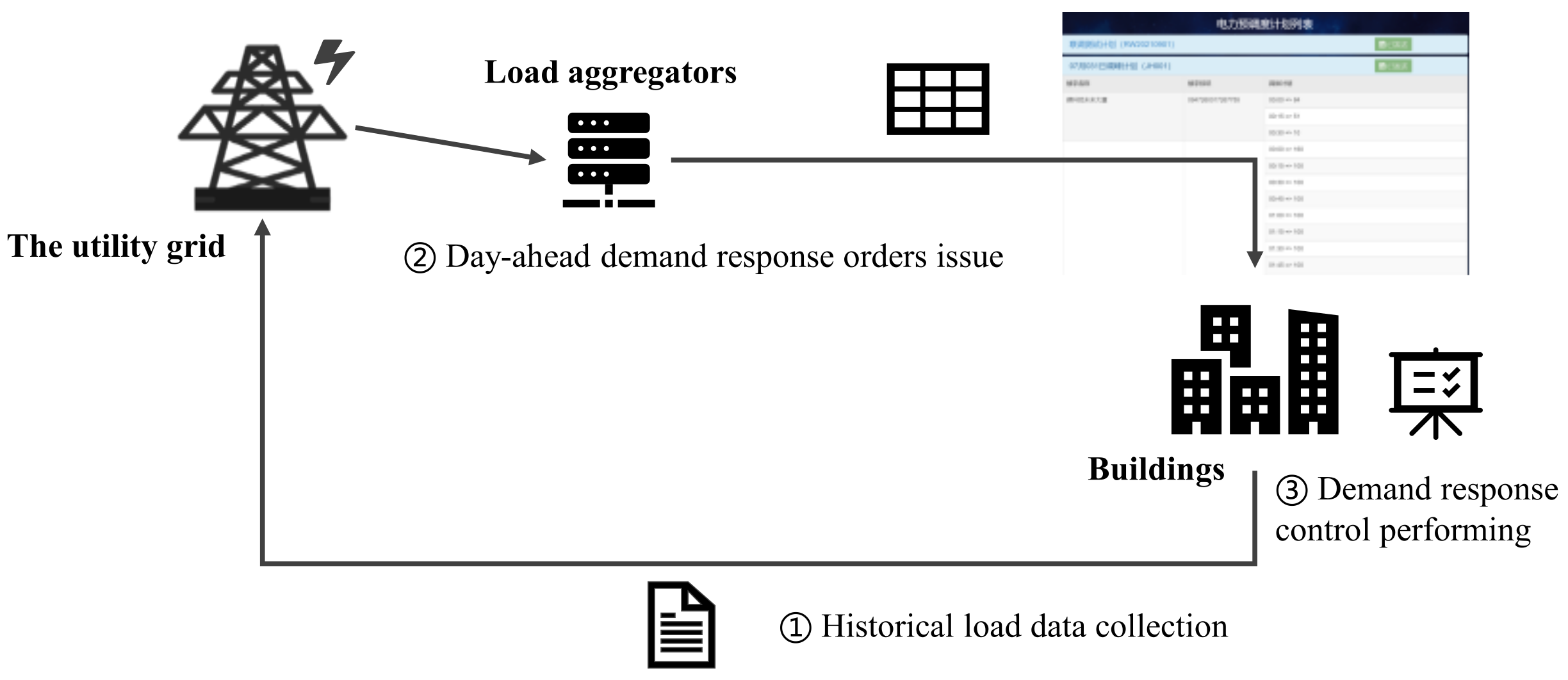
Demand response service from the grid consists of the conventional demand response and the ancillary service. In price-based programs, conventional demand response aims to load shifting by changing users’ electricity usage in a certain period. Ancillary service aims to increase the reliability of the grid when electricity demand surges suddenly. Fast responses, such as frequency regulation and peak clipping, are usually conducted while incentive-based programs are adopted [17]. Buildings and the belonging energy systems provide DR services mainly of the conventional type whose process is illustrated in Figure 1. Demand response is a program of three participants: (1) the utility grid that generates electricity; (2) load aggregators who sell electricity and (3) buildings that use electricity. Firstly, the utility grid collects historical load data of buildings to evaluate the load shifting potential of buildings and determines rational DR targets based on that. Load aggregators then manage and guide the service program. They make and issue day-ahead DR orders or schedules for buildings according to the target received from the grid within local energy policy. Finally, buildings implement load control or energy management following those DR orders. The corresponding reward is earned by buildings when their performance satisfies DR requirements.
2.2. Target and Mechanism of Air Conditioning Control in Demand Response
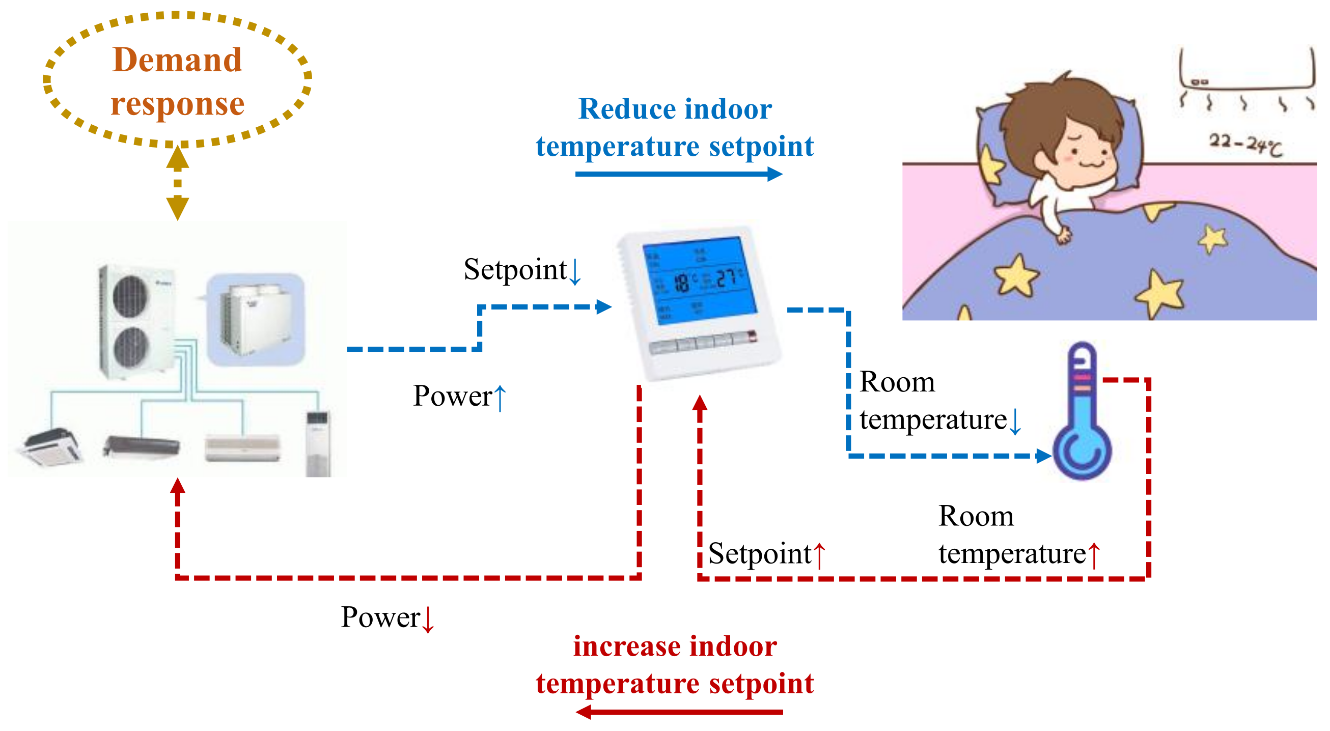
The magnitude of cooling capacity concerns the machine power in air conditioning systems, so that power shifting can be implemented by changing cooling capacity. The indoor temperature setpoint is one of the significant parameters to decide the cooling capacity of air conditioning. The basic mechanism of air conditioning control in demand response is shown in Figure 2. In the normal cooling process, the indoor temperature setpoint is reduced and cooling capacity increases, which raises the machine power. Room space is cooled down while the temperature is reduced, and indoor comfort is guaranteed. In the demand response process, the indoor temperature setpoint can be increased within a certain range while the change of room temperature satisfies the comfort requirement. Cooling capacity and machine power are reduced and the response target is achieved. This simple control process can be conducted by the majority of air conditioning systems in markets. Thus, it is an effective method that is valuable to be practiced and promoted in building demand response events.
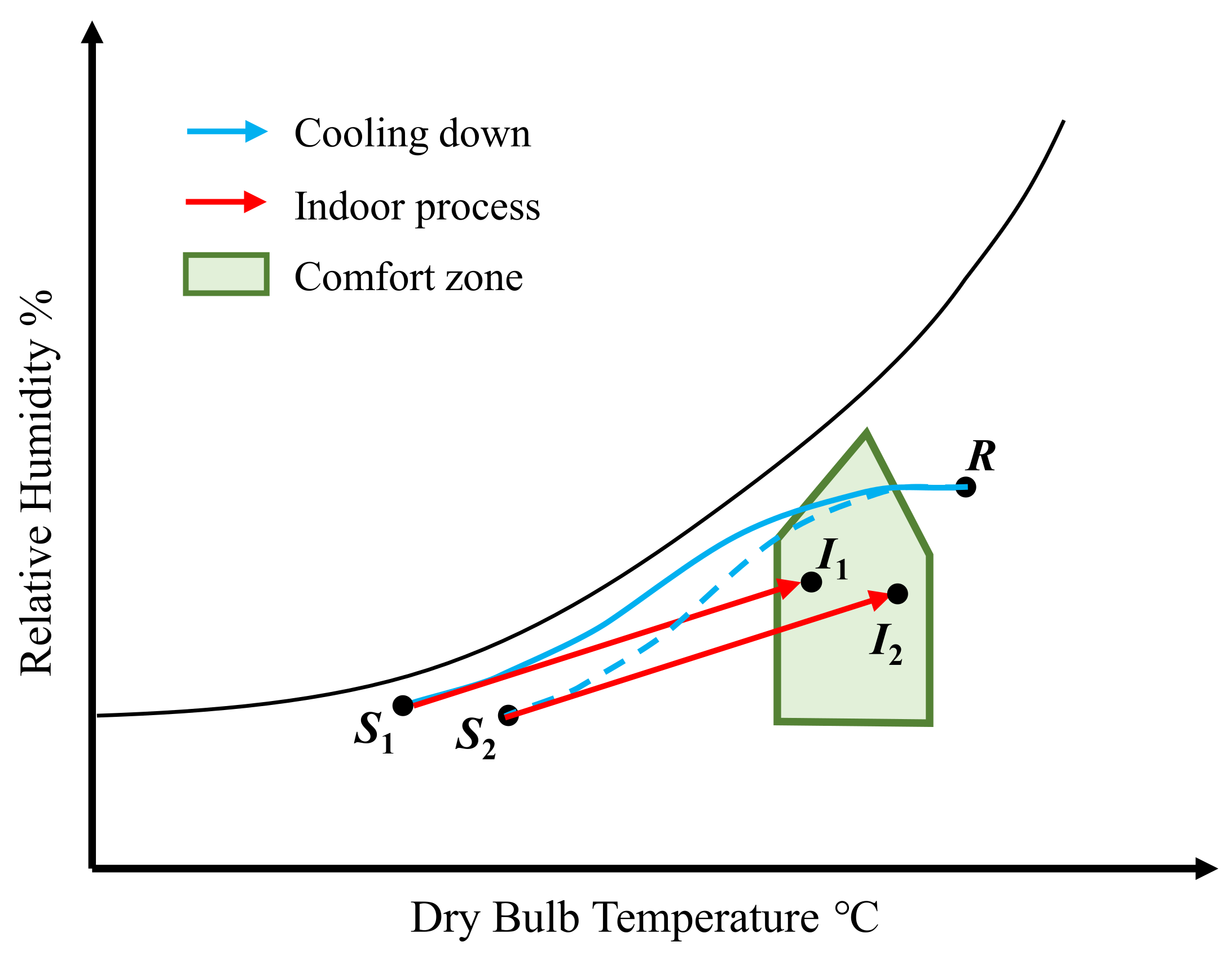
Figure 3 shows the air-handling process on the psychrometric chart with different temperature setpoints. The indoor unit cools the return air down to its apparatus dew point (R→S1). The cooled supply air is then heated and humidified to indoor air condition in the room (S1→I1). When the setpoint is increased, the cooling capacity of the indoor unit drops, and its corresponding apparatus dew point raises, so that return air is cooled down to S2. The air experiences the same reheat process and becomes the indoor condition I2. Indoor air conditions are within the comfort zone even the enthalpy of condition I2 is higher than condition I1.
3. Methodology
3.1. Prediction Model of HVAC Load
In the thermal equilibrium state of a room, the cooling capacity provided by HVAC equals heat gains from all sources, which is shown Equation (1). QH is the heat gain caused by the temperature difference between outdoor and indoor. QC is the heat gain caused by indoor thermal capacity. Qgen is the heat gain caused by the indoor heat source. Three assumptions considering both rationalities of engineering application and modelling simplification are made in this study as follows:
(1) Both sensible and latent cooling loads increase indoor air temperature and humidity, which become part of indoor thermal capacity. Therefore, the heat gain QC includes indoor sensible and latent cooling load;
(2) The coefficient of performance (COP) of a VRV with variable frequency drive varies with negligible range, i.e., 10%, in working conditions. It is assumed that the COP is a constant in modelling;
(3) The primary air unit, or fresh air system, is not considered in this proposed method. So that the effects of humidity, which is mainly caused by outdoor air, are neglected.
In detail, QH concerns the difference between outdoor temperature Tout and indoor temperature Tin,0 in the beginning, and QC concerns the difference between indoor temperature Tin,0 and setpoint of air conditioning Tset. Heat gain from the heat source usually remains unchanged as Pgen while the cooling capacity QAC can be simplified and estimated as the product of load PAC and COP. Thus, Equation (1) can be converted to Equation (2), while A and B are heat gain coefficients caused by temperature difference and thermal capacity, respectively. Indoor temperature reduces in the cooling process while temperature Tin,τ in time τ can be estimated in Equation (3). The air conditioning load should not be larger than the maximum value (Equation (4)).
3.2. Demand Response Program
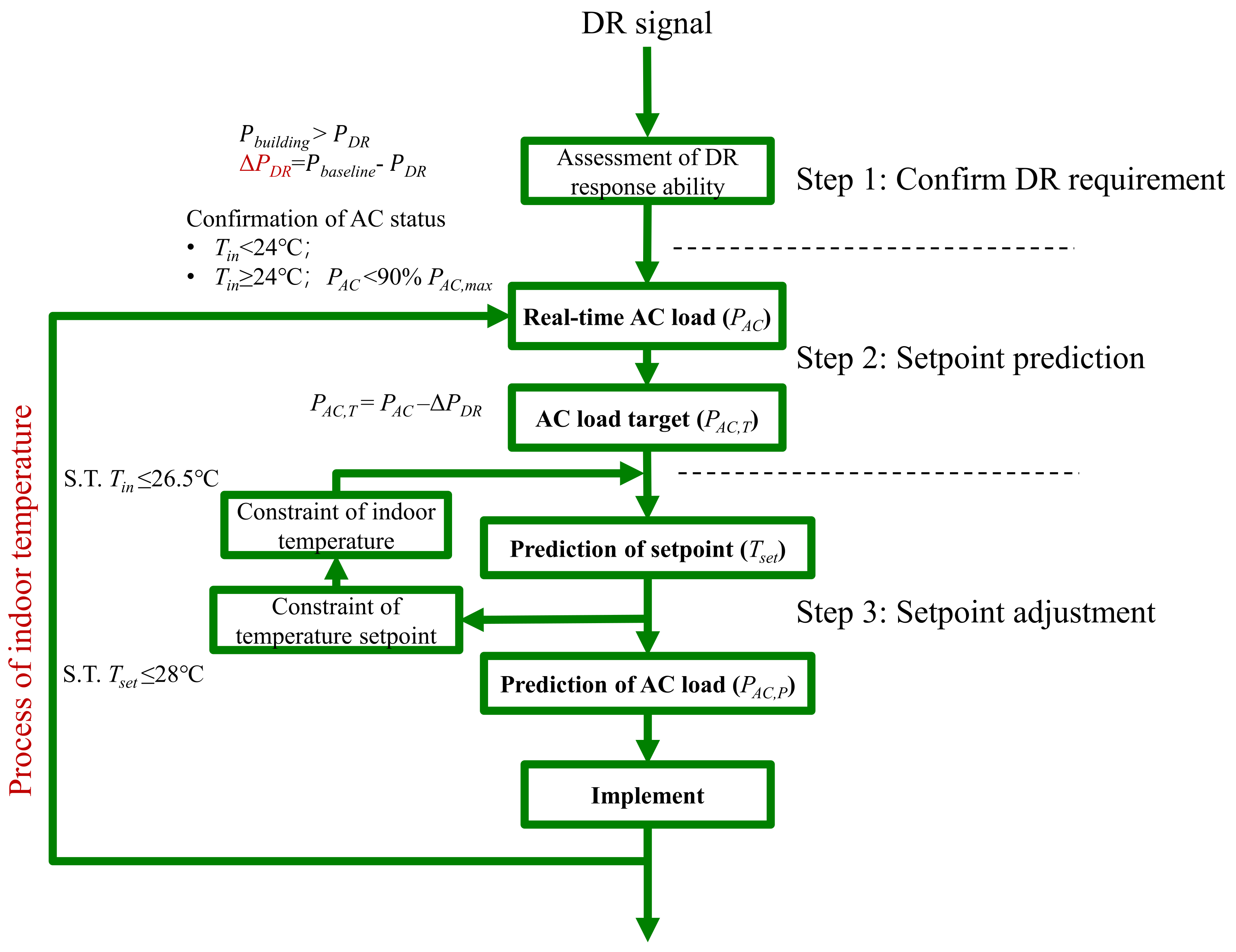
The demand response program can be divided into three steps as shown in Figure 4: confirm DR requirement, indoor temperature setpoint prediction, and indoor temperature setpoint regulation.
3.2.1. Confirm DR Requirement
When DR event is issued, (1) the response target PDR; (2) the building load Pbuilding; (3) the HVAC power PAC at the time are collected. Define DR requirement ΔPDR as the load which needs to be reduced to achieve DR target PDR (Equation (5)). If ΔPDR > 0, building demand response is required; if ΔPDR < 0, no action is performed. Whether HVAC participates in the DR event depends on two factors. ① When indoor temperature Tin < 24 °C which means that the room is cold enough. At this time, the HVAC cooling load can be reduced when indoor thermal comfort is satisfied ② When indoor temperature Tin ≥ 24 °C and HVAC load PAC < 90% PAC,max, which means that HVAC has not reached the maximum load while load reduction can be implemented. HVAC control can be adopted in the DR event in the above conditions.
3.2.2. Prediction of Indoor Temperature Setpoint
The basic idea of HVAC control is to reset the indoor temperature setpoint Tset which results in the HVAC load changing while building load adjustment can be achieved. The responding Tset under the DR requirement can be predicted using the above model. The target HVAC load PAC,T, which should be a positive value, can be estimated by Equation (6). The indoor and outdoor temperatures (Tin,0, Tout) at this moment should be collected while the time parameter τ should be set as 5 min.
3.2.3. Regulation of Indoor Temperature Setpoint
Indoor thermal comfort ought to be satisfied and the limitations of the HVAC setpoint should be considered during the DR event. The setpoint should be reset as 28 °C if the prediction value exceeds the upper limit, while it should be reset as 26 °C if the indoor temperature exceeds the upper limit of thermal comfort. HVAC load PAC,P at this time is predicted by using Equations (3)–(5). The HVAC control strategy is implemented when the predicted load PAC,P is smaller than the current load PAC.
4. Description of Test Site
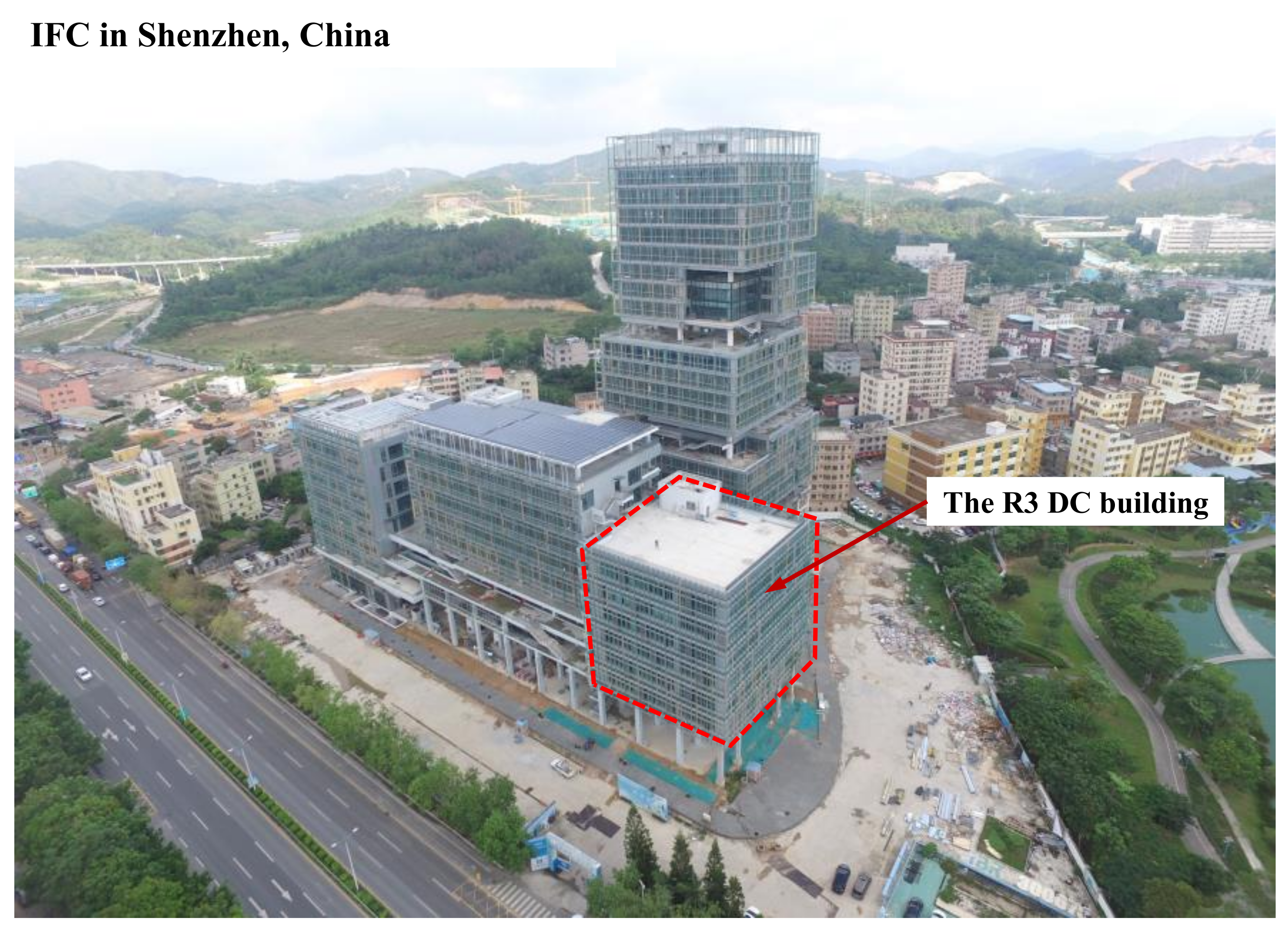
The IBR Future Complex (IFC) is a net-zero energy demonstration building located in Longgang District, Shenzhen, China, with a gross floor area of 62,523 m2 (as shown in Figure 5). The R3 block is a typical office building with a medium scale of 6259 m2. Original direct current (DC) power system is adopted to construct the building energy system which makes this block to be an efficient smart building. DC distribution technology to supply DC power for electric appliances, such as lighting, air conditioning, plug-in appliances, etc. With the utility grid, solar PV and BES as power sources, a building microgrid system is developed to satisfy the requirements of human activities and environmental comfort [18].
The R3 office area has six floors, each of about 660 m2, requiring a maximum cooling capacity of 99 kW. VRV air conditioning systems whose indoor units can be controlled independently by users are adopted for cooling. With a rated load of 10.5 kW, the maximum cooling capacity and heating capacity of the VRV air conditioning are 33.5 kW and 37.5 kW, respectively. Each floor in the R3 block is served by three VRV air conditioning units which consist of an outdoor unit and several indoor units to keep the space thermal comfort. Variable frequency compressor (VFC) is used in air conditioning units and outputs different cooling capacities by changing its frequency according to different demands so that the machine load is reduced as a consequence.
The IFC participates the Virtual Power Plant project led by China Southern Power Grid (CSPG), which aims to promote buildings to provide demand response services and achieve peak shaving goals of the utility grid by implementing an incentive-based program. The demand response service provided by IFC in this case is a day-ahead dispatch plan, which determines the power control target for different periods in a day according to the historical building load and issues scheduling instructions every 15 min on the previous day. In this mode, building users can be informed of the control objectives in advance and have enough time for preparation. The completion and execution of this demand response scenario are relatively high. From the perspective of the incentive mechanism, building users earn 2.4 USD (10 times the electricity tariff) for every 1 kWh electricity saved on the premise of achieving load control target, which helps users earn large profits.
5. Results and Discussion
5.1. Model Validation
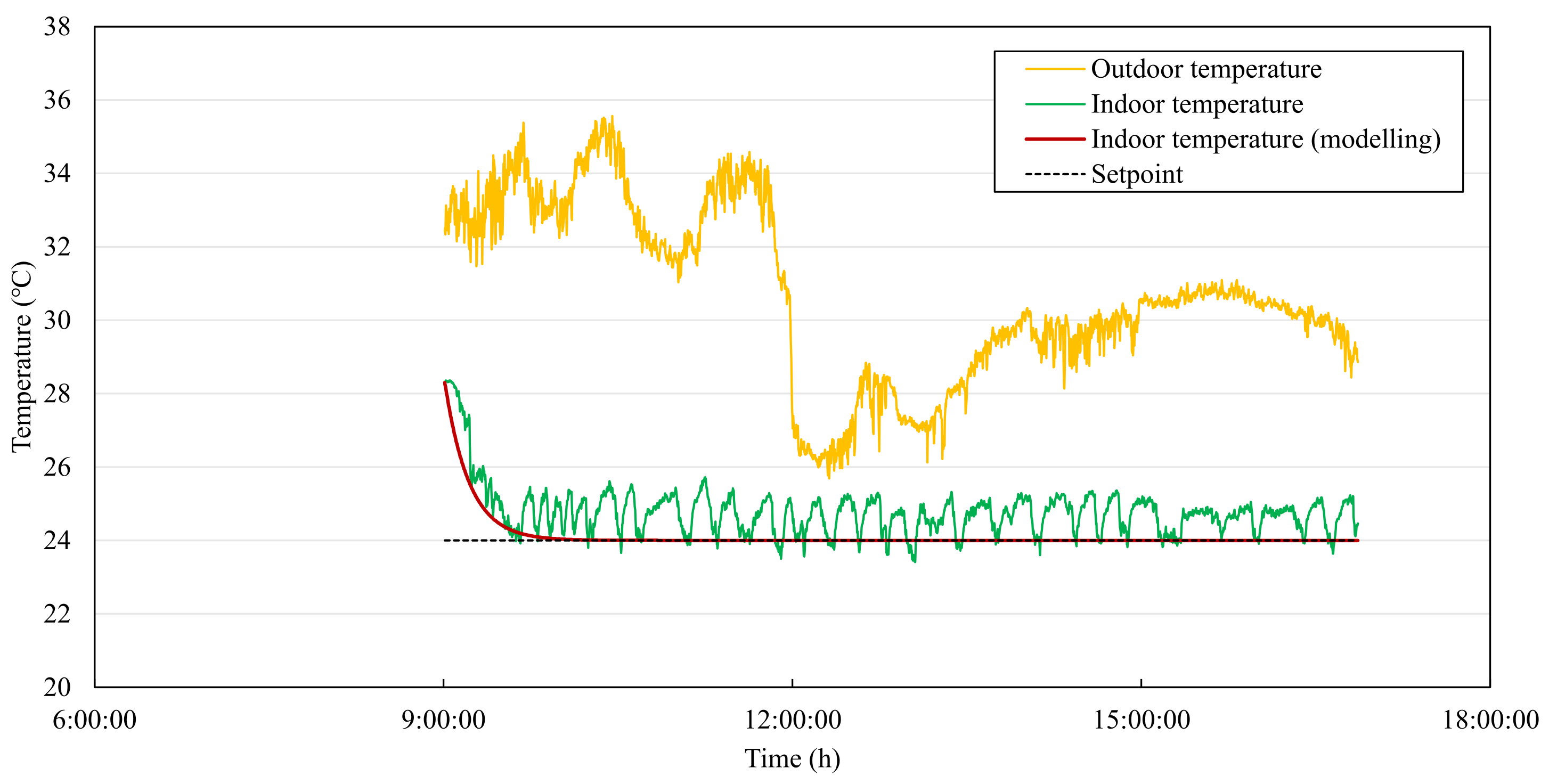
Figure 6 shows the measurement of indoor temperature, outdoor temperature, setpoint and the modelling result of indoor temperature during a cooling process. It can be seen that the indoor temperature rapidly drops to the set temperature of 24.00 °C and fluctuates within a certain range. The modelling value also drops to the set temperature and remains unchanged thereafter. In fact, human activities, periodic operation of equipment, and control process of HVAC system result in indoor temperature fluctuations, which cannot be reflected by a prediction model. From the perspective of cooling time, both measured value and modelling value reached 24.24 °C in 35 min (within a deviation of less than 10%), which means that the model can accurately predict the stabilization time of temperature in the cooling process.
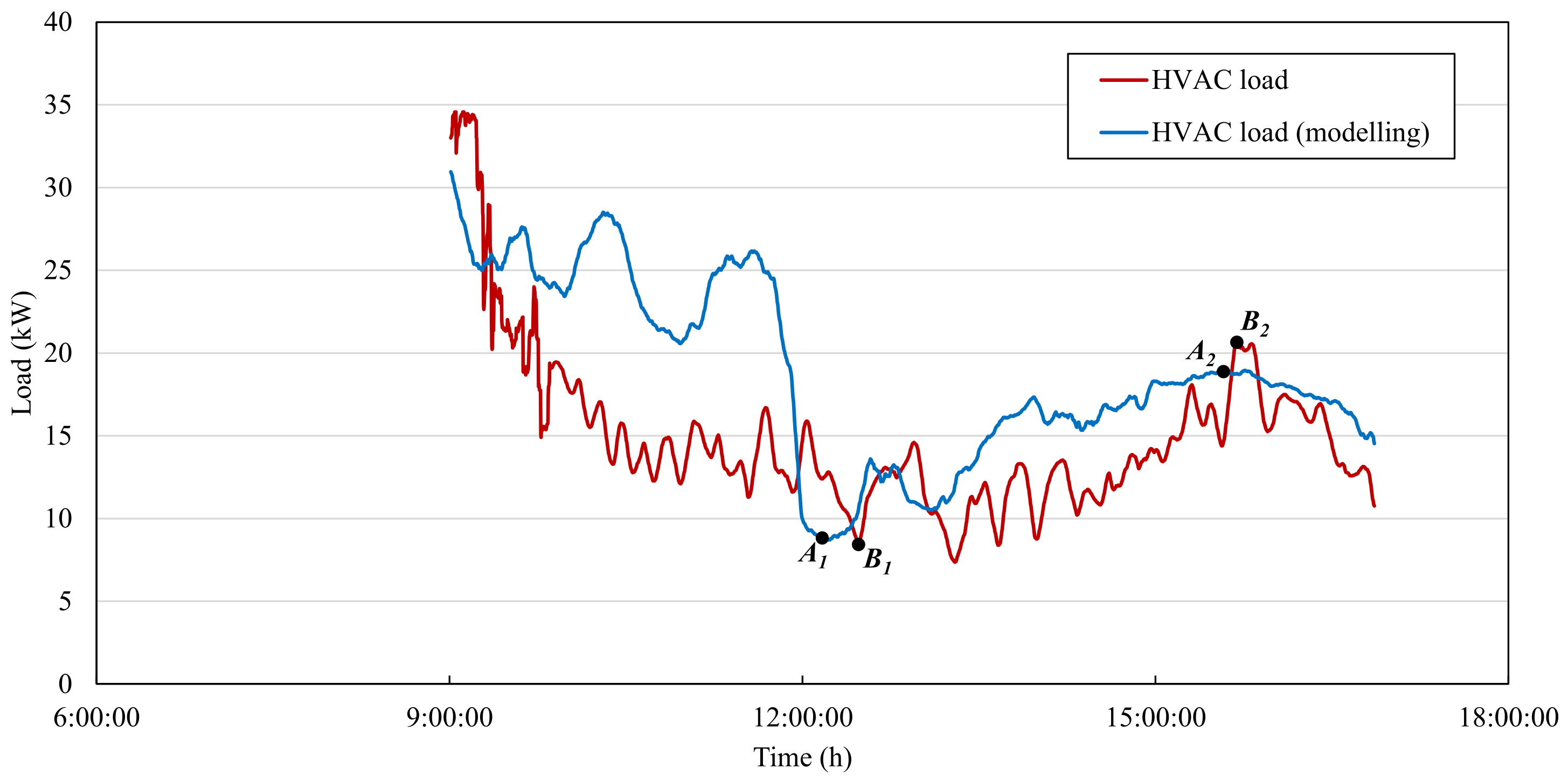
The comparison between the modelling result and measurement of HVAC load is shown in Figure 7. When the indoor temperature is cooled to a constant level while the outdoor temperature is changing, the predicted HVAC load is affected by the variation of outdoor temperature according to Equation (2). The load modelling results are consistent with the fluctuation of outdoor temperature. The measured HVAC load experiences the same rising and falling trend of the modelling results with periodic fluctuation, which is caused by the intermittent control of the electronic expansion valve. The modelling results have discrepancies with the measurement in the cooling process, which can only be solved by using a more accurate VRV model, but this does not affect analyzing and concluding this study. When the modelling load drops to the minimum value A1 of 7.46 kW in 12:19, the measured value drops to point B1 of 8.32 kW in 12:28. The time difference between those two points is 9 min while the value difference is 2.8%. When the modelling load rises to the peak value A2 of 19.50 kW in 15:41, the measured value rises to point B2 of 20.35 kW in 15:40. The time difference between those two points is 9 min while the value difference is 2.7%. Although the prediction model cannot predict the fluctuation of HVAC load, it still has a certain accuracy in predicting the peak value and corresponding time.
5.2. Performance of HVAC Response in DR Event
5.2.1. Response Time
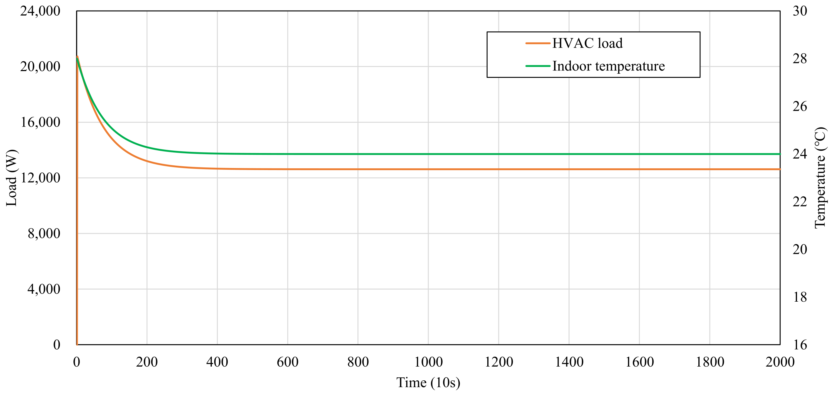
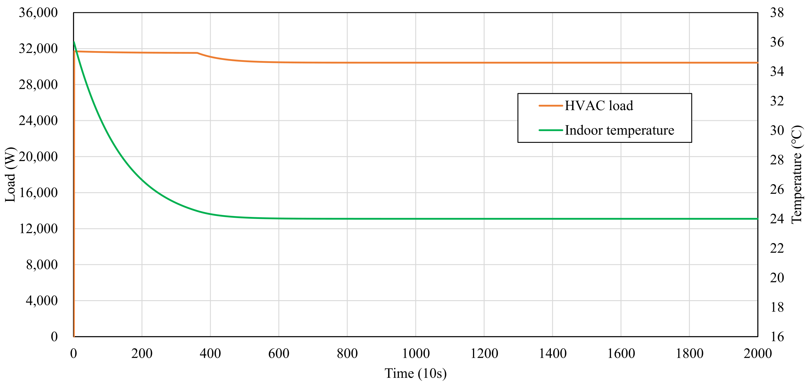
With initial indoor and outdoor temperature and HVAC setpoint, the load prediction model simulates the process of cooling and outputs profiles of indoor temperature and HVAC load. Figure 8 and Figure 9 show the cooling process when the setpoint is 24 °C and outdoor temperatures are 28 °C and 36 °C, respectively. It can be seen that at the beginning, abundant cooling capacity/HVAC load is required since the indoor temperature is higher than the setpoint. With the accumulation of indoor cooling capacity, indoor temperature and HVAC load gradually decrease. Finally, the indoor temperature drops to the setpoint and the HVAC load remains stable. When the temperature difference between indoor and outdoor is 4 °C (Tout is 28 °C), the indoor temperature drops to the stable value in about 2100 s (35 min); when the temperature difference is 12 °C (Tout is 36 °C), the indoor temperature drops to the stable value in about 4200 s (70 min). Results indicate that the duration to reach another cooling equilibrium, i.e., the response time of temperature regulation, is related to the temperature difference and varies in the range between 35 and 70 min.
5.2.2. Magnitude of HVAC Load
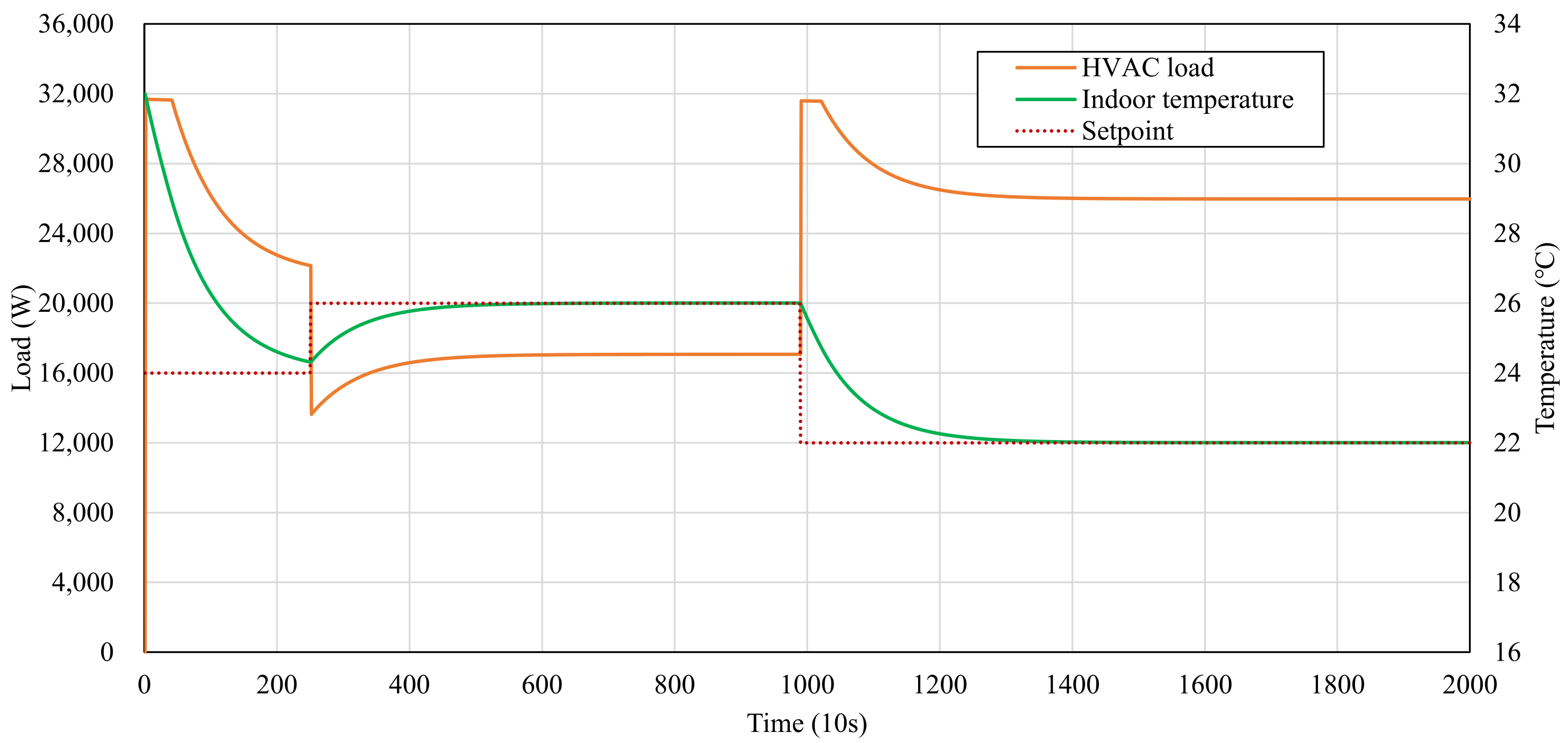
In the case of room cooling, the setpoint is regulated while HVAC load and temperature response profiles are predicted as shown in Figure 10. The setpoint is 24 °C at the beginning, the indoor temperature drops rapidly from 32 °C, while the load decreases after maintaining full power for a period of time. When the setpoint rises to 26 °C, the HVAC load drops rapidly because of the reduction of cooling demand and rebounds to 17.1 kW when indoor space reaches another thermal equilibrium. The HVAC load is 5.1 kW lower than 22.2 kW before regulating setpoint, which is about 16.0% of its rated load. When the setpoint drops to 22 °C, the HVAC load increases to maximum due to the surge of cooling demand. When the indoor thermal condition reaches equilibrium again, the HVAC load maintains 26.0 kW, which is about 28.3% of its rated load.
It can be seen that the HVAC load can be changed by regulating the indoor setpoint, which indicates that this control method can be used to implement building demand response. According to the modelling results, when the outdoor temperature remains stable (or fluctuates within a small range), the HVAC load changes by 8% for every 1 °C regulation of the temperature setpoint.
5.3. On-Site Test of DR Method
Based on the Virtual Power Plant (VPP) project of IFC, the DR method is implemented in the VRV air conditioning system, and the performance of this application is tested and analyzed. Servers of the Building Automation System (BAS) receive the DR target as well as load information of the building energy system from WAN and then predict the setpoints for each VRV using the proposed model. The control signal, i.e., the setpoint, is sent to the corresponding VRV by a decentralized controller using RS485. The setpoint of the indoor unit is changed and the reaction of indoor conditions is monitored by BAS as performance feedback. Characteristics of the HVAC system, cooling demand and corresponding effects of the tested building are listed in Table 2. The schedule and order of the DR method between 11:00 and 18:00, 19 November 2021, are shown in Table 3.
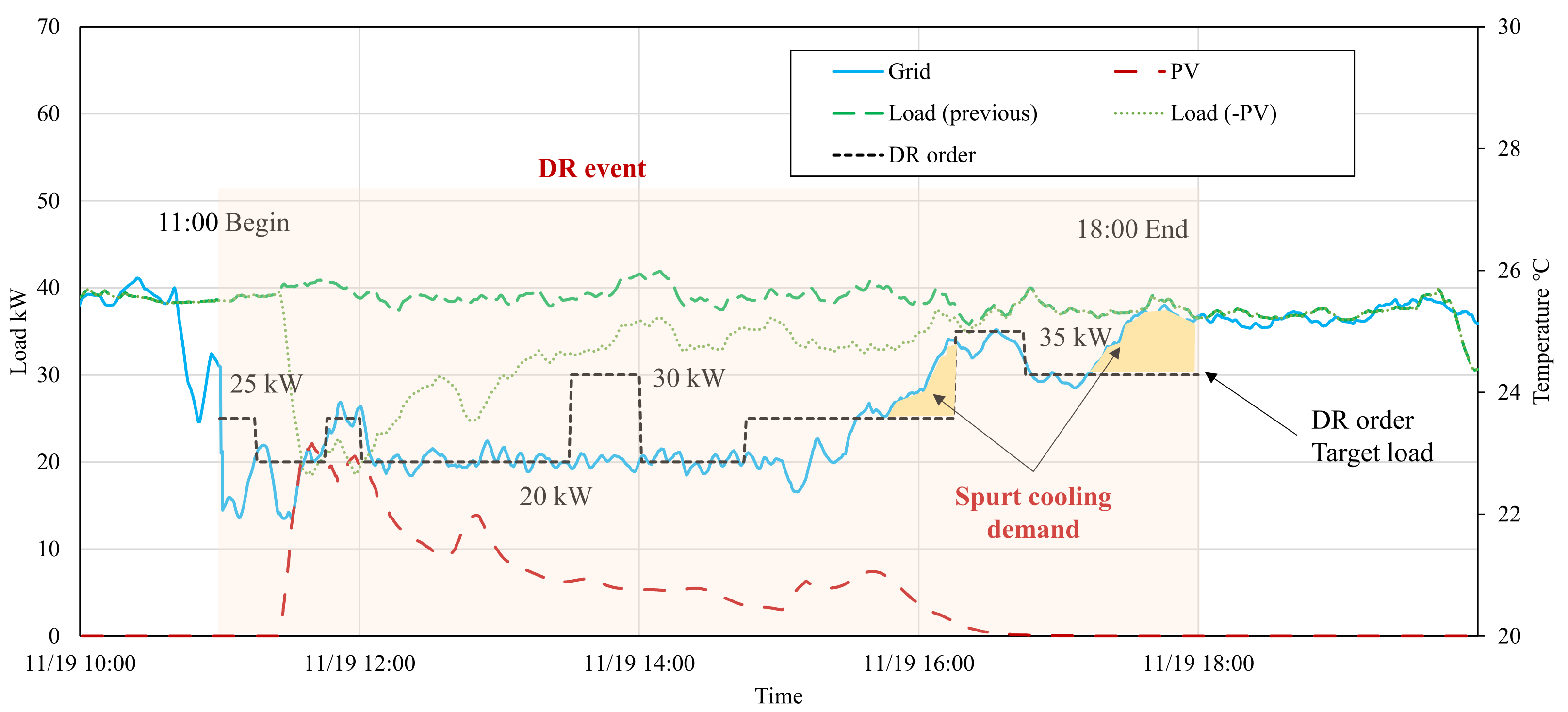
With the implementation of the control strategy, load curves of the building during the DR event are shown in Figure 11. The green solid line represents the electricity demand curve of a building without any DR method when the indoor temperature is aimed to be cooled down to 22 °C. The red solid line represents solar PV power generation which operates at the beginning of the test. The actual grid load of a building without the DR method, which is equal to building load minus PV generation, is calculated and presented as the green dotted line. The blue solid line indicates the building load implementing the DR method.
Comparing the building load and the DR control target, it can be found that the load is reduced blew the target while control results are as expected most of the time. At the beginning of the DR event, due to large load, reduction is required, the control strategy increases HVAC setpoints and results in a sharp drop of the building load. The building load is reduced to 15 kW, which is much smaller than the target of 25 kW. At 11:45, the HVAC load boosts on small scale, but the DR control strategy still limits the load variation according to DR order until 15:45.
After 15:45, the DR control strategy is unsuccessful in two periods of time. From 15:45 to 16:15, the building load starts to rise and exceeds the DR target, but it is then controlled at 35 kW and further at 30 kW. However, after 17:00, the building load continues to rise and exceeds the target again. The reason should be that the cooling demand increases due to the surge of indoor activities in these two periods of time, while the control strategy cannot generate enough sufficient load reduction. It is necessary to further modify the load prediction model for estimating more accurate HVAC setpoints to achieve expected load regulation.
Comparing the building load before and after the DR control strategy, the load reduction as a result of the control strategy can be obtained. It can be seen that the building load is reduced by 15–25 kW compared with that before regulation, and 61.1 kWh of electrical energy is saved during the DR event. According to the proposed incentive awarding of VPP, USD 2.4 will be paid for every kW reduction and USD 0.17 will be saved for every kWh energy saving. The building owner earns USD 58.39 in this DR event in total. The benefit of this DR method increases to USD 175.17 if the control strategy is adopted in the whole building, which covers 70% of the energy fee in the peak time of a year. It is a promising technique with substantial benefits for building demand response.
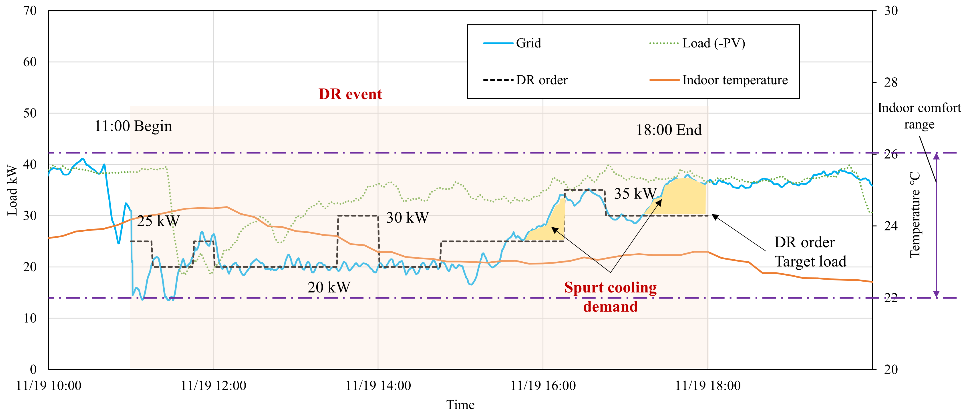
The indoor temperature changes during the DR event are shown in Figure 12. It can be seen that the temperature is controlled in the range of 22–26 °C, which fulfills the indoor comfort requirement. In the initial stage of the DR event, the HVAC setpoint is raised for load reduction which results in temperature raising. After reaching thermal equilibrium at 12:00, cooling capacity is sufficient and the indoor temperature begins to drop. At 16:00, the people activities and cooling load are rising. The indoor temperature increases slowly but still within comfort range because of the corresponding increase of HVAC cooling generation.
6. Conclusions
The present study proposes a building demand response method by controlling common air conditioning systems (HVAC). The key technology of this method is to regulate the indoor temperature setpoint of HVAC, and the electricity load will be regulated by the original HVAC control program as consequence. A modelling approach is used to predict HVAC load when the setpoint is changed, and a control procedure is developed to implement this DR method. An on-site test conducted in VRV HVAC systems of a demonstration building is implemented to validate the feasibility of the proposed method. Results show that it is a feasible technology to achieve building demand response goals by regulating the temperature setpoint of HVAC systems to change building load. The practical application case shows that during the DR event, this method reduces the building load by 15–25 kW, which is about 40% of the HVAC rated load, compared with that before regulation. The energy saving in 7 h is 61.1 kWh while the energy consumption is 166.8 kWh, which indicates that 26.8% of energy is reduced in DR events. From the perspective of economic benefits, the maximum awarding of this application can cover 70% of the energy fee in the peak time of a year. It is able to incentive building owners to attend DR services of the utility grid and reduce carbon emission by energy saving.
This proposed method can be adopted for almost HVAC systems with basic feedback control functions and communication protocol in buildings. Therefore, it is more suitable for promotion in existing engineering projects that need to provide demand response services. A load prediction model for a specific HVAC system must be reformed considering building functions and thermal characteristics in method application. More experiments with high cooling demand in summer cases should be conducted to validate this method, and the HVAC load prediction model should be further improved based on site measurements in future works.
Author Contributions
Methodology, J.K.; Project administration, Y.L.; Software, S.W.; Supervision, Y.L.; Visualization, S.W.; Writing—original draft, J.K.; Writing—review and editing, T.M. All authors have read and agreed to the published version of the manuscript.
Funding
The research presented in this paper is financially supported by the National Key Research and Development Program of China through the Grant 2019YFE 0111500.
Acknowledgments
Appreciation is given to the collaborative research projects of Shenzhen Institute of Building Research Co., Ltd and Shanghai Jiao Tong University.
Conflicts of Interest
The authors declare no conflict of interest.
References
- Zhang, D.; Wang, J.; Lin, Y.; Si, Y.; Huang, C.; Yang, J.; Li, W. Present situation and prospect of renewable energy in China. Renew. Sustain. Energy Rev. 2017, 76, 865–871. [Google Scholar] [CrossRef]
- Cai, W.G.; Wu, Y.; Zhong, Y.; Ren, H. China building energy consumption: Situation, challenges and corresponding measures. Energy Policy 2009, 37, 2054–2059. [Google Scholar] [CrossRef]
- Javed, M.S.; Song, A.; Ma, T. Techno-economic assessment of a stand-alone hybrid solar-wind-battery system for a remote island using genetic algorithm. Energy 2019, 176, 704–717. [Google Scholar] [CrossRef]
- Ma, T.; Yang, H.; Lu, L. Development of a model to simulate the performance characteristics of crystalline silicon photovoltaic modules/strings/arrays. Solar Energy 2014, 100, 31–41. [Google Scholar] [CrossRef]
- Kang, J.; Wang, S. Robust optimal design of distributed energy systems based on life-cycle performance analysis using a probabilistic approach considering uncertainties of design inputs and equipment degradations. Appl. Energy 2018, 231, 615–627. [Google Scholar] [CrossRef]
- Siddiquee, S.M.S.; Howard, B.; Bruton, K.; Brem, A.; O’Sullivan, D.T.J. Progress in Demand Response and It’s Industrial Applications. Front. Energy Res. 2021, 9, 673176. [Google Scholar] [CrossRef]
- Zhu, Q.; Wang, Y.; Song, J.; Jiang, L.; Li, Y. Coordinated Frequency Regulation of Smart Grid by Demand Side Response and Variable Speed Wind Turbines. Front. Energy Res. 2021, 9, 576. [Google Scholar] [CrossRef]
- Kwag, H.-G.; Kim, J.-O. Reliability modeling of demand response considering uncertainty of customer behavior. Appl. Energy 2014, 122, 24–33. [Google Scholar] [CrossRef]
- Siano, P. Demand response and smart grids—A survey. Renew. Sustain. Energy Rev. 2014, 30, 461–478. [Google Scholar] [CrossRef]
- Xu, J.; Yan, C.; Xu, Y.; Shi, J.; Sheng, K.; Xu, X. A Hierarchical Game Theory Based Demand Optimization Method for Grid-Interaction of Energy Flexible Buildings. Front. Energy Res. 2021, 9, 500. [Google Scholar] [CrossRef]
- Shan, K.; Wang, S.; Yan, C.; Xiao, F. Building demand response and control methods for smart grids: A review. Sci. Technol. Built Environ. 2016, 22, 692–704. [Google Scholar] [CrossRef]
- Wang, S.; Xue, X.; Yan, C. Building power demand response methods toward smart grid. HVACR Res. 2014, 20, 665–687. [Google Scholar] [CrossRef]
- Wang, S.; Tang, R. Supply-based feedback control strategy of air-conditioning systems for direct load control of buildings responding to urgent requests of smart grids. Appl. Energy 2017, 201, 419–432. [Google Scholar] [CrossRef]
- Tang, R.; Wang, S.; Gao, D.-C.; Shan, K. A power limiting control strategy based on adaptive utility function for fast demand response of buildings in smart grids. Sci. Technol. Built Environ. 2016, 22, 810–819. [Google Scholar] [CrossRef]
- Wang, H.; Wang, S.; Tang, R. Development of grid-responsive buildings: Opportunities, challenges, capabilities and applications of HVAC systems in non-residential buildings in providing ancillary services by fast demand responses to smart grids. Appl. Energy 2019, 250, 697–712. [Google Scholar] [CrossRef]
- Wang, H.; Wang, S.; Shan, K. Experimental study on the dynamics, quality and impacts of using variable-speed pumps in buildings for frequency regulation of smart power grids. Energy 2020, 199, 117406. [Google Scholar] [CrossRef]
- Ma, Y.; Chen, X.; Wang, L.; Yang, J. Investigation of Smart Home Energy Management System for Demand Response Application. Front. Energy Res. 2021, 9, 648. [Google Scholar] [CrossRef]
- Kang, J.; Hao, B.; Li, Y.; Lu, Y.; Li, Y. Practice of DC Distribution System-based Building Microgrid: A Case of IBR. In Proceedings of the 12nd International Symposium on Heating, Ventilation and Air Conditioning (ISHVAC 2021), Seoul, Korea, 24–26 November 2021. [Google Scholar]
Figure 1.
Typical process of building demand response.

Figure 2.
Process of air conditioning control in demand response.

Figure 3.
Process of air conditioning control in demand response.

Figure 4.
Program of HVAC control in DR event.

Figure 5.
IFC in Shenzhen and the R3 DC building.

Figure 6.
Modelling result and measurement of indoor temperature.

Figure 7.
Modelling result and measurement of HVAC load.

Figure 8.
HVAC response in cooling (Tout = 28 °C/Tin = 24 °C).

Figure 9.
HVAC response in cooling (Tout = 36 °C/Tin = 24 °C).

Figure 10.
HVAC response in cooling with variable indoor temperature setpoint.

Figure 11.
Variation of grid load in DR event.

Figure 12.
Variation of indoor temperature in DR event.


Table 1.
List of parameter values.
| Parameters | Unit | Value | Description |
|---|---|---|---|
| J/K | 9,616,420 | Heat capacity of the room | |
| s | 1440 | Fitting coefficient in function | |
| s | 759 | Fitting coefficient in function | |
| A | W/K | 6678 | Heat gain coefficient caused by temperature difference |
| B | W/K | 12,670 | Heat gain coefficient caused by room heat capacity |
| Pgen | W | 11,150 | Power of indoor heat source |
| COP | — | 3.0 | Coefficient of performance |
Table 2.
Operation statement and responding description in the test.
| Items | Description | Operation Statement | Effect |
|---|---|---|---|
| VRV air conditioning | VRV units are used in 7/8F. The rated load and cooling capacity are 10.5 kW and 33.5 kW. | All VRV units are opened in 7/8F. Indoor temperature setpoint is 22 °C in normal scenario without any control. | Maximum load of VRVs is 52.5 kW which has great potential for demand response. |
| People activity | One of the heat sources. More activities need much cooling capacity. | Workshops, exhibition preparation, study. | Activities result in fluctuation of cooling load and VRV’s operation. |
| Environment | Cooling is needed in subtropic regions. | Max. temperature is 25 °C while PV generates. | Uncertain of PV output results in fluctuation of building load. |
Table 3.
Schedule and order in demand response.
| Time | 11:00–11:15 | 11:15–11:45 | 11:45–12:00 | 12:00–13:30 | 13:30–14:00 |
| Load Target (kW) | 25 | 20 | 25 | 20 | 30 |
| Time | 14:00–14:45 | 14:45–16:15 | 16:15–16:45 | 16:45–18:00 | |
| Load Target (kW) | 20 | 25 | 35 | 30 |
Publisher’s Note: MDPI stays neutral with regard to jurisdictional claims in published maps and institutional affiliations. |
© 2022 by the authors. Licensee MDPI, Basel, Switzerland. This article is an open access article distributed under the terms and conditions of the Creative Commons Attribution (CC BY) license (https://creativecommons.org/licenses/by/4.0/).
Share and Cite
MDPI and ACS Style
Kang, J.; Weng, S.; Li, Y.; Ma, T. Study of Building Demand Response Method Based on Indoor Temperature Setpoint Control of VRV Air Conditioning. Buildings 2022, 12, 415. https://doi.org/10.3390/buildings12040415
AMA Style
Kang J, Weng S, Li Y, Ma T. Study of Building Demand Response Method Based on Indoor Temperature Setpoint Control of VRV Air Conditioning. Buildings. 2022; 12(4):415. https://doi.org/10.3390/buildings12040415
Chicago/Turabian StyleKang, Jing, Shengjie Weng, Yutong Li, and Tao Ma. 2022. "Study of Building Demand Response Method Based on Indoor Temperature Setpoint Control of VRV Air Conditioning" Buildings 12, no. 4: 415. https://doi.org/10.3390/buildings12040415
Note that from the first issue of 2016, this journal uses article numbers instead of page numbers. See further details here.