
A Review of Mathematical Models of Building Physics and Energy Technologies for Environmentally Friendly Integrated Energy Management Systems


1
School of Mathematics, Frontiers Science Center for Mobile Information Communication and Security, Southeast University, Nanjing 211189, China
2
School of Engineering and the Built Environment, Edinburgh Napier University, Edinburgh EH11 4BN, UK
3
Delft Center for Systems and Control, Delft University of Technology, 2628 CD Delft, The Netherlands
*
Author to whom correspondence should be addressed.
†
These authors contributed equally to this work.
Buildings 2022, 12(2), 238; https://doi.org/10.3390/buildings12020238
Submission received: 31 December 2021
/
Revised: 14 February 2022
/
Accepted: 15 February 2022
/
Published: 18 February 2022
Abstract
:The Energy Management System (EMS) is an efficient technique to monitor, control and enhance the building performance. In the state-of-the-art, building performance analysis is separated into building simulation and control management: this may cause inaccuracies and extra operating time. Thus, a coherent framework to integrate building physics with various energy technologies and energy control management methods is highly required. This framework should be formed by simplified but accurate models of building physics and building energy technologies, and should allow for the selection of proper control strategies according to the control objectives and scenarios. Therefore, this paper reviews the fundamental mathematical modeling and control strategies to create such a framework. The mathematical models of (i) building physics and (ii) popular building energy technologies (renewable energy systems, common heating and cooling energy systems and energy distribution systems) are first presented. Then, it is shown how the collected mathematical models can be linked. Merging with two frequently used EMS strategies, namely rule-based and model predictive controls, is discussed. This work provides an extendable map to model and control buildings and intends to be a foundation for building researchers, designers and engineers.
1. Introduction
The building sectors account for around 36% of energy consumption and 39% of carbon emissions of the globe [1]. Thus, improving the building energy performance by increasing the use of clean and renewable energy systems is a promising direction to realize resource conservation and face climate change. With the development of the concept of ’nearly zero-energy building’, some novel technologies, such as renewable energy resources, onsite storage systems and environmentally friendly devices in buildings, have gained more interest [2].
As an alternative to producing electricity from fossil fuels, renewable energy resources based on solar and wind provide clean and low-cost energy for buildings and have been increasingly used in recent years (Photovoltaic Panels (PVs), Solar Thermal Panels (STPs), Wind Turbines (WTs), etc.) [3]. The existing literature shows the generation model of solar and wind power under different weather conditions [4,5], as well as algorithms to maximize their usage ratio in buildings [6,7].
However, the inherent uncertainty and intermittence of renewable generation bring new challenges to the power systems. This means that the onsite renewable generation profile may not be consistent with the consumption profile in buildings. Hence, some energy storage technologies (electricity storage or thermal storage) are often used simultaneously with renewable resources as effective techniques to deal with the mismatch between renewable generation and local consumption [8]. Meanwhile, energy storage technology can improve energy flexibility and decrease the operation cost [9]. It is shown that a combination of renewable generation and energy storage systems can reduce up to 30% of the annual cost and increase up to 29% of the self-consumption proportion of renewable energy [10].
Environmentally friendly technologies with a high Coefficient of Performance (COP)—for example, heat pumps and Combined Heating and Power (CHP)—have also been increasingly studied and developed [11,12]. These devices can be combined with water-based energy distribution systems that allow for low-temperature heating [13] and high-temperature cooling [14] to cover the heating and cooling demand of the buildings.
With so many technologies co-existing in one building, a smart Energy Management System (EMS) solution to operate and make them profitable for users needs to be considered. There are generally two kinds of EMS: passive EMS and active EMS [15]. The former improves the energy efficiency in buildings by predicting the load curves and influencing users’ awareness [16], whereas the latter monitors and controls the elements of building energy systems via a set of well-designed control strategies [17]. EMS has been researched and applied to span from the device level [18] and the single building level [19] up to the building community level [20]. Typical EMS implementations for buildings include defining a series of control rules dependent on the energy or electricity price thresholds [21], executing mixed integer optimization under time-of-use electricity price and incentive policy [22], establishing a game theory model between user behaviours and the electricity price policy [23] and using a bionic algorithm, such as genetic algorithms [24] or particle swarm optimization [19], to optimize the operation of household appliances. The EMS can also interact with the grid side to determine the incentives [25] or reduce the energy bill [26]. For the grid operators, this interaction helps to protect the power grid from the risk of power blackouts by reducing the peak-to-average ratio [27].
1.1. Research Motivation: Integration
Studying complex EMSs in buildings requires the use of building simulation and programming tools separately or collectively. Building simulation tools are mature techniques to analyze the building performance under different targets; for example, energy consumption and thermal comfort. Several building simulation tools (e.g., TRNSYS, EnergyPlus, IDA-ICE) are widely developed to provide a precise model for the buildings and technologies [11,28,29,30,31]. However, all building simulation tools face a similar situation when integrated with an EMS: they are only able to account for the modeling of buildings (and sometimes also a few standard equipment), but they cannot be merged in a seamless way with the EMS based on different control strategies. As a matter of fact, usually the data from simulation tools must be collected into another programming tool (e.g., MATLAB, Python) to complete the control part. This difficulty becomes more apparent when the prediction is taken into account in an EMS. For example, an EMS covering energy flexibility conversion, routing and storage options was investigated in [32], where the modeling and control parts were carried out in TRNSYS and MATLAB separately. In addition, different EMSs for a community of buildings were studied in [11], sorted out into two parts: first, calculating each building heating energy demand by building simulation tools (TRNSYS or IDA ICE); then, using the data as input values into the programmed EMS in MATLAB. This strategy to undertake the simulation tools for building modeling and the programming tools for executing EMS strategies separately brings difficulties and challenges in setting up a framework, which increases the run time and may cause inaccuracies through the final results. This may especially be inconvenient when exploring an analysis of complex scenarios (such as buildings integrated with energy technologies and EMS).
1.2. Related Works
Different models of energy technologies have been proposed in the literature, cf. Table 1. However, coherent framework that can integrate all of these models in a unified way is still missing. The aforementioned framework should describe how the different technologies interact with each other, and how they can be operated by the EMS (e.g., by selecting certain thresholds or a certain power). A possible solution to the issue of integration is to merge physics-based mathematical models to create comprehensive building energy systems [33]. Then, corresponding EMSs can be easily coded and linked to such building energy systems models. Towards this purpose, bottom-up load models of the residential space heating and cooling load, Domestic Hot Water (DHW) load, appliances and equipment and electric vehicles have been developed and validated in [33]. However, these models were based on traditional heating technologies; as a result, this approach does not cover renewable energy resources and efficient environmentally friendly technologies, such as heat pumps. Another EMS framework focused on microgrid control and optimization based on objectives, constraints and optimization methods was reviewed in [34], but most popular and environmentally friendly technologies and energy distribution systems were not discussed.
Although the techniques for modeling HVAC systems were reviewed in [84,85], it is unclear how the component models can be connected to model the whole energy systems in buildings. In fact, some studies have shown that the integration between modeling and control requires dedicated mathematical models, e.g., modular approaches to connect different devices [86,87]. Another example is the integrated HVAC and DHW production systems discussed in [88], which are given without presenting the models. It is mentioned that there is a great challenge to minimize the mismatching between the design and real energy performance, which highlighted the requirement for unified modeling methods for multi-energy systems. Taking into account the aforementioned concerns, setting up a whole framework that includes both the mathematical models and control strategies for buildings installed with environmentally friendly technologies is still an open problem. Most importantly, this integration should fit different configurations in different buildings.
1.3. Contribution of This Study
This study contributes computationally efficient models suitable for the EMS design for buildings. The aim is to describe a selective and integrated approach. The mathematical models presented in this work can be connected to construct different energy systems in different buildings. In this way, the models of building physics and energy systems cover all types of technologies popularly installed in buildings. The experiments to verify the selected models are not presented here, but they are referred to the validations in the reviewed studies; for example, by comparing with the results of building simulation tools [56] or measurements data [74,89,90]. The discussed models are expandable and integrable. Therefore, a direction is to combine them and to analyze the building level performance. Besides, this paper provides a whole map to establish EMS in buildings based on the different layout and installed technologies, and contributes to the further research of EMS design for researchers, designers and engineers.
The rest of this paper is organized as follows. Section 2, Section 3 and Section 4 present a review of the assemblable mathematical models for building physics, heating and cooling energy systems and onsite energy generation and storage. Section 5 discusses two common EMS strategies, namely Rule-Based Control (RBC) and Model Predictive Control (MPC). Section 6 summarizes the framework and gives concluding remarks.
2. Building Physics
Models for building physics can be categorized as white-box, black-box and grey-box [91]. The first approach is adopted by most building simulation tools, such as TRNSYS and EnergyPlus: this approach consists of estimating the demand and consumption of a specific building based on weather data, building envelope, installed technologies and consumption profiles totally based on the physical relationships. Examples of black-box models are neural networks or autoregressive moving average models, in which, the mathematical relationships between inputs (e.g., weather data) and outputs (e.g., energy consumption) are purely based on collected data. A grey-box method is a hybrid approach combining white-box and black-box models, since it is based on physical formulations (e.g., heat transfer laws) with parameters tuned by measured data.
A detailed review of white-box modeling and black-box modeling was presented in [84,85]. These reviews mention that the white-box models are often developed based on a number of assumptions and parameters, which causes a complex construction process and low accuracy. On the other hand, the accuracy of black-box models usually depends on the types of the selected methods. A large number of training data are required to develop the black-box models, with a relatively lower generalization capability. This means that the generated relationships are valid for a specific building but unsuitable for other different building configurations. To achieve a framework that takes into account both building physics and heterogeneous energy technologies, the grey-box approach based on the widely used thermal Resistance and Capacitance (RC) network model is one of the most adopted approaches. An RC model exploits the analogy between the energy flow and electric flow, since a capacitor represents an accumulation of energy, whereas the resistance represents a dissipation of energy. The two main factors that influence the accuracy and complexity of an RC network are its spatial resolution and order. Spatial resolution simply refers to the option of aggregating all rooms as a single zone, or describing each room with a separate RC model. The order of an RC model refers to the number of lumped elements in the model; for example, one capacitor (1C) [92] or two capacitors (2C) [93,94]. The second option is more capable of describing phenomena such as the thermal capacity of the air and building fabric [95]. According to their order, the most standard RC models are the so-called 2R-1C [96] or 3R-2C [97]. The 3R-2C model is usually suggested as a trade-off between complexity and accuracy, and examples reported in the literature include a large retail store building with 28 zones in California [98] and an office building with 7 zones and 33 surfaces [99], indicating that this model can be adjusted for buildings with a wide range of sizes.
Apart from the energy flow and heat exchange, infiltration due to leaks and cracks in the building envelope has a non-negligible influence on the total energy demand [100]. Measuring the infiltration rate in buildings is essential to control and manage the energy consumption and improve indoor thermal levels. Various methods were developed to achieve this value [101]. For simplicity, the infiltration can be assessed by the airtightness, i.e., the leakage–infiltration ratio of buildings [102]. This value expresses a linear relationship between the air leakage rate and the infiltration rate, and is considered over a period of time.
The schematic representation of a general multi-zone 3R-2C network is shown in Figure 1, with each node in the model representing a point of interest. Once the layout of one floor in the building is determined, the multi-zone 3R-2C network is expressed as follows:
This model is applied for a variety of buildings and the coefficients can be calculated based on the information of the building envelope. It can also be reduced to a single-zone model by assuming .
3. Onsite Energy Generation and Storage
This section concludes a review of the mathematical models of onsite energy generation (PV, STP, WT, CHP) and energy storage units (battery, HWST, PCM).
3.1. Photovoltaic Panel
A PV produces electricity based on solar energy. The generated power is influenced by the weather conditions, among which, the ambient temperature and solar radiation are the main factors. For simplicity, most models assume that the total radiation is falling on the solar array, and the angle of incidence is not considered [26]. A linear model used by [37] expresses the generated power (W) as:
where (%) indicates the conversion efficiency, which is typically equal to 16%, and G (W/m) is the solar radiation. An alternative model to (5) is proposed in [6]:
where () and () are the temperature sensitivity of the photovoltaic generated current and voltage, their typical values are %/ and , (W) is the nominal power of the PV in the standard test conditions ( W/m, , AM = 1.5) and () is the cell temperature, which can be estimated by [41]:
The model (5) is a linear model, whereas (6)–(8) constitute a quadratic one. It is possible to tune the parameters of both models in such a way that their results are similar in a certain operating region. However, the linear model is able to estimate the generation for a wider range of cell temperatures, whereas the quadratic one predicts the generation around the nominal temperature more accurately. A combination of them can be used, e.g., the quadratic model is used when is the nominal temperature and the linear model is used when is large.
3.2. Solar Thermal Panel
A STP produces thermal heat with solar energy. Solar radiation and ambient temperature are also the dominant factors of the STP performance. The usable heat (W) produced by a flat plate STP can be calculated with the Hottel–Whillier–Bliss equation [103]:
where (m) refers to the area of the collector, (%) is the heat removal efficiency factor, (%) is the transmittance absorptivity, (W/(m K)) is the heat loss coefficient, (kg/s) is the water mass flow rate, () and () is the inlet and outlet water temperature and (J/(kg K)) is the specific heat of water. It is assumed that , , are constants for a given collector, water flow rate (typically 0.005 kg/(s m)) and fluid inlet temperature [104]. In particular, the technical characteristics are assumed to be %, %, W/(m K), which are typical values for double-glazed flat-plate collectors [105]. The model (9) calculates the usable heat produced by STP based on a function of its area and solar radiation, and is simplified by assuming the coefficients as constants.
The combination of PV and STP forms a new technology called photovoltaic thermal collectors, which simultaneously converts solar energy into heat and electricity [106]. It is noted that the electricity and heat production efficiency of photovoltaic thermal collectors is lower than that of the separate PV or STP, but that its overall efficiency is higher [38].
3.3. Wind Turbine
A WT is a local generation device based on wind energy. It works when the wind speed (m/s) is within a certain range (larger than cut-in velocity (m/s) and less than cut-off velocity (m/s)). In fact, the power (W) generated by the WT can be calculated by the following piece-wise function of the wind velocity [107]:
where (W) is the rated electrical power and (m/s) is the rated wind speed. Other approaches calculate in an alternative but analogous way [26]:
where () is the air density, (m) is the blade radius and (%) is the power coefficient. It is assumed that , which is the air density at sea level and 25 and %, which is a typical value in the literature. These two formulations represent a simple way to integrate data of wind velocity in the generation of wind energy.
3.4. Combined Heating and Power
CHP or micro-CHP is a class of equipment in which the waste heat of an electrical generator is collected to cover thermal loads [47]. A CHP system usually consists of the following parts: (1) prime mover, e.g., combustion turbine, engine or microturbine; (2) electric generator; (3) heat recovery unit, which transforms wasted heat to reusable thermal energy.
An analytical dynamic model for a micro-CHP with a Stirling engine taking into consideration the start-up and cool-down periods and partial load performance was developed in [108], and an experimentally validated model of an internal-combustion-engines-driven, natural-gas-fueled device based on a product of Marathon engine systems ecopower was studied and tested in [47], demonstrating that the generated heat and electricity power were nearly linear functions of the engine speed within the operating range. Another empirical model for the engine was polynomials presented in [41], and is suitable for a wider range of CHP rated power. According to this model, the electricity and thermal heat generation efficiency is estimated by:
where (%) is the part load ratio calculated by:
where (W) and (W) are the generated and rated electricity power. Then, the relationships between the fuel input (W) and electricity and thermal outputs are:
The model directly focuses on the relationship between fuel consumption and produced energy, The overall system efficiency is usually used to assess the performance of a CHP, which is the sum of produced electricity and thermal heat divided by the total fuel energy input [109].
3.5. Battery
A battery provides the potential to purchase or store electricity during off-peak hours and to sell or use electricity during peak hours in buildings. The models for batteries derived from the literature can be classified into linear and nonlinear ones [110]. The recommended model in this framework is the linear one [53]:
where (W/s) and (W/s) are the charging and discharging rates, and they cannot be positive simultaneously for the safe operation and long life span of the battery. (W/s) and (W/s) are the limited charging and discharging rates for the safe operation of the battery, S (W) is the state of charge, (%) is the loss proportion due to energy leakage and (%) and (%) denote the charging and discharging efficiency. Typically, , and and are usually 20% and 80% of the total battery capacity. This model is easy to implement compared with nonlinear models: it only requires knowledge of the initial state of charge of the battery [34].
3.6. Hot Water Storage Tank
The HWST is a cost-effective technology for thermal heat storage. Tanks based on stratification give a higher efficiency than a fully mixed tank of the same size [111]. In this work, a stratified HWST that enables a high temperature layer at the top and a low temperature layer at the bottom of the tank is used.
The modeling methods of a stratified HWST can be categorized in terms of its dimension. Two-dimensional [112,113] or three-dimensional [114,115] solutions based on Computational Fluid Dynamics (CFD) techniques are accurate but require long calculations. As a result, the one-dimensional tank models are highly regarded, and some studies have shown that their accuracy can be comparable to CFD models [54]. Different approaches and configurations have been proposed for one-dimensional modelings, such as incorporating inflow or outflow buoyancy and a mixing process [55], a node-mixing model for a pressurized water tank with two immersed heat exchangers [116], a mixing factor parameter determined by experimental measurements [56] or including PCM to improve the storage capacity of the tank [89].
The schematic representation of a stratified HWST with five nodes (one node represents one layer) is presented in Figure 2. Different energy technologies can be integrated with it. The energy balance equation in each layer is expressed as follows:
The size and configuration of this tank is similar to that presented in [11]. The top layer provides DHW for the occupants, and the lower layer is connected to Heating, Ventilation and Air Conditioning (HVAC) for space heating. Technologies such as GSHP, ASHP and micro-CHP are installed in nodes 1–4. An electric heater is used in node 5 to ensure the minimum temperature of DHW, which is typically 55 ; for example, in the Finnish building regulations [117]. Domestic Cold Water (DCW) or city water that is around 15 enters the bottom layer with the same speed of DHW. Let (), denote the temperatures of five layers from the bottom to the top. The analytical model based on energy balance equations validated by [55,89] for HWST is written as follows:
where the heat transfer through the vertical conduction of node i, represented as (W) can be modeled as [89,116]:
where (m) is the cross sectional area between the neighbouring nodes, (W/(m K)) is the thermal conductivity of water and (m) is the height of each layer. The heat transfer between water in node i and the inner surface of the tank (W) can be calculated with Newton’s law of cooling:
where the evolution of the case temperature () is:
where (W) is the heat loss of the tank calculated by:
It is worth mentioning that considering the connection between HWST and other heating or cooling technologies is what allows us to build a multi-device framework combining several technologies.
3.7. Phase Change Materials
PCMs are becoming more popular and approachable for thermal storage due to their high storage density during the phase change process. The most common type of PCM is the solid–liquid one [118], which can be installed in an HWST [66,89], water-based heating/cooling system [119,120], ventilation system [121] or building structure [60,122]. Different kinds of PCM are chosen according to their physical characteristics, such as their heat convective coefficient and phase change temperature, for different application requirements. Water or air usually takes the role of the heat transfer fluid in the charging and discharging process.
The effective heat capacity method [60] and the enthalpy method [89] are two common ways to model the thermal storage process of PCM [123]. The charging performance of a PCM tank based on thermodynamic laws was studied in [66], whereas a two-dimensional PCM model in HWST based on the enthalpy method was studied in [89]. The model of the PCM-to-air heat exchanger can be found in [122]. An interesting comparison between the effective heat capacity method and enthalpy method can be found in [123]. It is shown that the two methods are both effective in predicting the charging or discharging time and air temperature, whereas the effective heat capacity method is more accurate in modeling the component temperatures of PCM. Thus, both of them can be used when studying the system level performance, but the effective heat capacity method is preferred when focusing on PCM behaviour.
In this study, it is assumed that the PCM has a unified temperature, demonstrating a high performance with no complex calculations [121]. The effective heat capacity method is expressed as [64]:
where (J/(kg K)) and (J/(kg K)) are the specific heat of the PCM under a solid and liquid state, respectively, (J/kg) is the latent heat of fusion, () is the PCM temperature, () and () are the melting ranges and (W) is the heat transfer to PCM. The alternative enthalpy method is expressed as [89]:
where (kg/m), (m) and (J/kg) are the density, volume and specific enthalpy of the PCM material. These two recommended models can support different application scenarios: it is necessary to couple the target technology (e.g., HWST) with the appropriate capacity (or enthalpy) coefficient resulting from the models above. This also allows us to combine different technologies into one framework.
4. Heating and Cooling Systems
According to the literature review, environmentally friendly heating and cooling energy technologies are inefficiently instructed in the state-of-the-art; therefore, they are taken into account in this section. They can be integrated to form the water-based energy system in buildings based on the water flow rate and/or temperature with the intention of the modeling process in a programming environment together with the control laws. This section concludes a review of the mathematical models of the environmentally friendly heating technologies (ASHP, GSHP), environmentally friendly cooling technologies (DEC, IEC, CC, AC, CCHP) and energy distribution systems (hydronic (HR) heating system, chilled beam, Radiant Cooling System (RCS)).
4.1. Heating Technologies
4.1.1. Air Source Heat Pump
ASHP transfers heat from the heat source to the heat sink depending on its mode, and this provides more potential for energy saving. Two types of ASHP are common nowadays [124]: one is the air-to-air heat pump, which transfers the heat extracted from outside air to inside air, and the other is the air-to-water heat pump, which transfers the heat extracted from ambient air to the HR heating system inside the building. The latter type is more convenient to integrate with the HWST and the water-based heating and cooling systems if they are available. Thus, this type of ASHP is considered for this study.
Heat pumps are usually modeled in terms of COP. The COP is defined as the ratio between the produced thermal power and consumed electric power. It is a widely used description for the efficiency of heat pumps and chillers. The COP of ASHP has been modeled in various ways, such as being a constant independent on the ambient temperature, supply water temperature and other factors [71], or a linear model of the ambient temperature [70]. The most accurate but complex model is a quadratic form, as studied in [125], taking into account the ambient temperature, normalized compressor power and returned water temperature to the condenser. A linear approximation of is used in this study [126]:
where () is the inlet water temperature. Then, the heating power (W) and outlet temperature () can be calculated by:
where (W) is the power consumed by the compressor and (kg/s) is the mass flow rate of water, which is usually assumed to be 0.5 kg/s. This model is a good trade-off between accuracy and complexity. It can be connected with other parts of the water-based heating systems and contributes to the whole framework.
4.1.2. Ground Source Heat Pump
GSHPs use ground temperature to warm or cool the circulating water in the system. Due to the fact that the ground temperature is more stable than the ambient air temperature, GSHP can usually achieve a better performance (i.e., higher COP) than ASHP.
The factors that influence the COP of a GSHP system include the type of ground heat exchangers (horizontal or vertical), soil condition, local climate, building load characteristics and system design and control optimization [65]. Again, the COP has been modeled as a constant [11], or dependent on meteorological information, such as solar radiation and the ambient temperature [127]. A field study conducted in hot summer and cold winter areas in China [128] indicated that the COP ranges from 1.95 to 4.35 depending on various outside conditions. A quadratic model for the COP of a solar-assisted GSHP was considered in [129], whereas the adverse influence of soil temperature evolution was quantified in [130], since the operation of GSHP caused variation in the soil temperature when the load was high. It is also shown that increasing the vertical length and the space between the exchangers can decrease the soil temperature variation. It is assumed that the soil temperature is constant in one month as a conclusion of the various proposed models, and that the quadratic model of based on the temperature difference between the soil and the outlet water is as follows [131]:
The operation of GSHP can be modeled similar to ASHP:
where (W) and (W) are the heating and consumed compressor power, and (kg/s) is the water mass flow rate, which is assumed to be 0.5 kg/s [12]. The modeling methods based on COP avoid the long calculations in the heat transfer models of ground heat exchanger; for example, in [132].
4.2. Cooling Technologies
Although novel cooling systems are continuously proposed as a combination of various technologies, exploring all of these combinations is outside the scope of this work. Therefore, a few popular technologies that are suitable for the aimed framework are carefully investigated.
4.2.1. Evaporative Cooling
Evaporative cooling is an efficient and sustainable way to cool the space in a hot and dry climate. It utilizes the evaporation process while the non-saturated water absorbs a large amount of heat from the air, increasing the air humidity and decreasing the air temperature simultaneously. Evaporative cooling is categorized as direct and indirect evaporative cooling (DEC and IEC) [133]. In DEC, water and air make contact directly, allowing the air to cool to wet bulb temperature, but the increased humidity of the outlet air may bring discomfort. In IEC, there is no direct contact between the water and air, allowing the air to cool to dew point temperature.
A mathematical model based on energy conservation, heat transfer and mass transfer for DEC was investigated in [134], calculating the total heat transfer with temperature difference and absolute humidity difference. This model is further simplified in [73] to improve the computational effectiveness:
where (%) is the effectiveness of DEC, (W/(m K)) is the convective heat transfer coefficient, (m) is the area of the heat transfer surface, (kg/s) is the mass flow rate of the air and (J/(kg K)) is the specific heat of the humid air, expressed as:
where (J/(kg K)) is the specific heat of the vapour, and (kg water/kg dry air) is the air humidity ratio of the inlet air (e.g., the ambient air). Typically, it is assumed that = 35 W/(m K), = 1 kg/s (the heat transfer coefficient is based on the air velocity), =1007 J/(kg K) and = 1868 J/(kg K). Then, the outlet air temperature and total cooling power (W) are:
where () and () are the temperatures of the inlet and outlet air respectively, and () is the wet bulb temperature of the air.
The Number of Transfer Unit (NTU) method, also referred to as the -NTU method, is used to deal with the situation where the outlet temperature is unknown, such as evaporative cooling systems and chilled beams. An IEC model based on a modification of this method [74] was proven to significantly reduce the computational complexity compared to the differential equation models based on physical calculations. This method assumed a linear relationship between the temperature of saturated air in the water film () and the enthalpy h (J/kg) within a small temperature range:
where the values of a and b can be fitted with the data in [135]. Then, the cooling power (W) is expressed as:
where () is the inlet air temperature to the dry passage, (J/kg) is the enthalpy of inlet air to the wet passage, (%) is the modified effectiveness and is calculated based on the modified cold and hot fluid heat capacity:
where (kg/s) and (kg/s) are the air mass flow rate in the wet and dry passage. is calculated based on a function of modified NTU values. For a parallel flow IEC, the function is:
For a counter flow IEC, the function is:
where the modified NTU values and capacity ratio are calculated by:
where (W/(m K)) is the convective heat transfer coefficient in the dry passage, (m) and (W/(m K)) are the combined thickness and thermal conductivity of the water film and thin wall between the dry and wet passages and (kg water/kg dry air) is the mass transfer coefficient in the wet passage. The typical parameter settings for a 0.25 m IEC are = 0.00098 kg/s, = 0.0014 kg/s and m. These two models are recommended for DEC and IEC since they can be used for different configurations without considering the dynamic energy transfer process.
4.2.2. Chiller
The cooling process of a chiller is similar to the inverse of the heating process of a heat pump. There are two kinds of chillers: absorption and compression chillers (ACs and CCs) [81]. The first type uses thermal heat to circulate the refrigerant around the system, so that it is profitable in the situation where heat can be available at low prices, e.g., the waste heat from the boiler. The second type uses a compressor to circulate the refrigerant. It is suitable for the situation where electricity is cheap and heat is expensive to achieve. COP is the common performance factor for chillers. Similar to the COP of heat pumps, the COP of chillers also can be modeled as a constant [136], a linear function of system states [137,138], a function of the part load ratio [139], a bi-quadratic function [80], polynomials [80] or an exponential function [79].
Four modeling methods for ACs, including a white-box, a grey-box and two black-box models, are compared in [79], indicating that the empirical models can offer a simple way to calculate the cooling capacity and COP without knowing the internal working fluid temperature. Six black-box models based on water-side data for CCs were compared in [80], showing that the bi-quadratic model and polynomial model had a better performance. An accurate linear COP approximation method of chillers was proposed in [137]: the inputs include the inlet and outlet water temperatures, source and sink temperatures and the cooling load. To avoid a large number of inputs that need extra measurements, COP models based on part load ratios are adopted in this work. The model for AC is presented in [41] as follows:
The model for CC is presented in [83] as follows:
where (%) and (%) are the part load ratios of AC and CC, and these two values usually range from 0.2 to 1 due to the minimum engine speed. (%) is the relative efficiency of correcting the COP of the chiller under different part load ratios, and (W) is the capacity of CC. Then, the cooling power and returned chilled water temperature can be calculated by:
The CCHP system is usually a combination of CHP and chillers. The generated energy by CHP in terms of electricity or heat can be supplied to chillers to provide cooling energy [44,140]. The connections and energy flows in a CCHP system are shown in Figure 3. The power generation unit produces electricity with fuel inputs (e.g., gas), and the recovered heat is collected. The generated electric power (W) and thermal power (W) can be calculated with the CHP model presented in Section 3.4. Then, the generated electricity and heat, possibly along with other supplements from energy storage devices or the grid, support the CCs or ACs. Thus, the final generated cooling power of CCHP can be calculated with the chiller model presented in Section 4.2.2 with the electricity or thermal inputs. The performance of CCHP is evaluated by the efficiency of the power generation unit and the COP of the chillers [41].
4.3. Energy Distribution Systems
The supplied energy is distributed into each zone by the hydronic distribution systems used in this research. The models of auxiliary systems (e.g, water pumps) placed between energy systems and distribution systems are not studied in this work.
4.3.1. Hydronic Heating Systems
HR heating is a popular heat distributed system as it is compatible with several energy sources, such as solar energy and heat pumps. Combining conduction and radiant technology, heat emitters, such as wall-mounted radiators and underfloor coils, emit radiant heat to provide heat [141]. The output power (W) of a HR radiator can be modeled as follows [142]:
where (kg) and () are the mass and averaged temperature of water inside the HR radiator, (m) is the area of the radiator and (W/K) is the heat transfer coefficient that depends on the temperature difference. For simplicity, it is assumed that the radiator surface and inside water have the same temperature, so that can be calculated as:
where (W/(m K)) is the convection coefficient, and (m) is the area of the radiator. The typical parameter settings of a low temperature HR radiator are W/(m K) and kg/(m s) [143]. This model is based on an energy balance equation and can be connected with the models of thermal storage or heating technologies presented in this work.
4.3.2. Chilled Beam
The chilled beam is a cooling distribution technology utilized in a wide range of types of buildings, such as industries, commercial buildings, households and even transportation vehicles. There are mainly two kinds of chilled beams: Passive Chilled Beams (PCBs) and Active Chilled Beams (ACBs) [144]. The schematic representations of them are shown in Figure 4 and Figure 5.
The PCB provides cooling power for buildings through natural convection. The rising warm air loses heat to the coils with chilled water and falls to cool the room. The cooling capacity of PCB is dependent on the temperature difference (typically 8–9 ) between the chilled water and indoor air, beam configuration and height of the roof [145]. Typically, the chilled water at 14 to 18 flowing through the coils at speed ranges from 0.02 kg/s to 0.2 kg/s and provides 20–40 W/(m K) cooling power [146].
Analytical PCB models based on CFD analysis can accurately predict the indoor airflow, air temperature and contaminant concentration [147], but they are time consuming. Alternatively, the simplified mathematical models that are easily implemented can be developed by a regression method. For example, a multi-variable regression model with the data from the CFD analysis for the coupled displacement-ventilation and PCB system was investigated in [148]. Another work based on similar methods with the data from experimental studies predicted the cooling capacity (W) based on part load ratios [90], expressing the models for a single chilled beam as:
and the model for multiple chilled beams in a large open office is:
where the subscript means the rating case, and the typical values are: W, kg/s and . These formulations simplified the calculation by avoiding the physical details in heat transfer and distribution, and have been used in a building level analysis in [149].
The ACB provides cooling power for the building through forced convection. The indoor air is inducted to flow across the coil with chilled water. Typically, the induction ratio is 1/4 and the cooling power is 100–200 W/(m K) [146]. The NTU model for ACB presented in [150] is proven to be accurate and easy to implement for modeling the cooling capacity and supplied air temperature compared with other accurate analytical models; for example, in [151], it expresses the total cooling power (W) by:
where (W) is the cooling power from the primary air:
where (kg/s) is the mass flow rate of the primary air flow, which is typically equal to 0.03 kg/s, and () and () are the temperatures of the primary air and exhausted air. (W) is the cooling power from chilled water, and is calculated by the NTU method:
where () is the inlet temperature of the chilled water, and (J/(kg K)) is the minimum heat capacity according to:
where (kg/s) refers to the mass flow rate of secondary air (i.e., induced air), which is the product of the induction ratio, and , (kg/s) is the mass flow rate of the chilled water, which is typically equal to 0.04 kg/s. (%) is the effectiveness parameter, which is a function of NTU, for the common application cases (NTU is less than 3) of cross-flow ACB, and an accurate approximation of is:
where is calculated with:
and NTU is defined as:
where (W/(m K)) is the overall heat transfer coefficient of the coil and (m) refers to the heat transfer area. The NTU model is recommended for the aimed framework since it shows a good correspondence with measured data without extensive calibrations and long calculations.
4.3.3. Radiant Cooling System
Another popular terminal cooling technology is the RCS. It is a broad concept that refers to a system where radiant heat transfer covers over half of the total heat transfer. The embedded surface cooling system, thermally activated building system and radiant cooling panels all belong to this concept [152]. It has been increasingly applied in a wide range of types of buildings due to its lower energy consumption and better thermal comfort compared to traditional air conditioners [153]. A simplified model of RCS was proposed in [154]: assuming that all masses in the room have temperatures close to the zone air and that the slab temperature is uniform, then the cooling power (W) is calculated as follows:
where (W/(m K)) is the heat transfer coefficient expressed by:
where () is the radiant surface temperature, and k is a constant depends on the emissivities of the panel. The values can be found in [155]; one typical value is 8. The dynamics of the slab temperature is:
where (kg) and (J/(kg K)) are the mass and specific heat of the radiant panel, (kg/s) is the water mass flow rate, () and () are the inlet and outlet temperatures of the panel and (%) is the fraction of the internal heat gain absorbed by the radiant panel. A typical value for is 0.08 kg/s for every 100 m pipe. The model is validated under weekly prediction and the complexity allows for its integration with a real-time MPC algorithm [154].
5. Energy Management System
In the previous sections, building physics and energy systems were discussed to create a framework for buildings equipped with several energy systems. In this section, the picture of the whole framework is completed by discussing how to control these technologies, i.e., EMS is investigated. Some popular control strategies are reviewed in the following stages of this work to show how to operate the technologies based on these models. This investigation reviews EMS approaches to categorize them in terms of their visions and usability.
A solution to enable EMS is to design a combination of computer-aided strategies to monitor and control building energy loads [156]. This system aims to improve the performance efficiency of the installed technologies, including the HVAC devices, onsite generation and storage systems, by operating them correctly. In this way, EMS allows buildings to achieve both their own objectives and those of grid suppliers based on the prediction of the energy generation and demand [157]. Two strategies are most frequently used to design the EMS: Rule-Based Control (RBC) and Model Predictive Control (MPC), respectively. This section examines the formulation of control problems and the concepts, approaches and comparison of RBC and MPC.
5.1. Rule-Based Control
RBC is a series of predefined decisions based on “IF-THEN” commands and real-time monitoring. The “IF” conditions of these commands often include some threshold values dependent on the difference between a reference value and the measured values (e.g., limited price and hourly energy prices). RBC is adjusted by determining the operation of energy systems (e.g., on/off of HVAC devices) based on a rule set. The control objectives are set to reduce the energy cost and energy consumption, for example.
RBC is most frequently used for cost reduction based on real-time energy prices. A multi-level RBC algorithm for a solar-assisted GSHP heating system was investigated in [158], showing that the EMS could select different energy technologies under the fluctuating real-time electricity price. Three different RBC approaches as examples, called momentary, backwards-looking and predictive control algorithms, were proposed and compared in [56] to control a GSHP heating system. It was shown that predictive control outperforms the others. The control rules in the three approaches were based on the comparison between the current Hourly Energy or Electricity Price (HEP) and a constant limiting price, the comparison between the current HEP and the median of the past HEP and the trend of future HEP, respectively. The typical methods to generate the price trend include a blocking-maximum subarray method, sliding-maximum subarray method and moving average [21]. Different definitions of price thresholds for RBC based on the location and length of the time window were discussed in [159]. The price thresholds can be calculated with either the bottom and upper percentiles, or deviations from the average prices of the time window. In addition to controlling the heating or cooling systems as discussed above, RBC was also employed for controlling the operation of multi electricity appliances and the storage system [160], the setpoint temperature of swimming halls [161], the concentration of educational office buildings [162] and the integrated operation of HVAC and blinds in office buildings [163] with similar rules. Occupancy patterns can also be taken into consideration when setting the rules, with the set-back and pre-cooling modes defined based on the occupancy profile [164].
Although some of the above studies showed an over 10% cost reduction under real-time electricity prices, there are still plenty of situations that do not provide real-time energy prices, leading to a lower economic potential by load shifting. As a result, RBC is also implemented to decrease the energy consumption. A rule set to preheat or switch off the equipment based on the historical data was defined in [165], and another one to control the operations of smart windows to minimize the solar flux and guarantee the illumination in cooling seasons was studied in [166]. A fast chiller power control was employed in [167] with the rule set to estimate the chiller power reduction and to reset the air temperature setpoint and chilled water distribution. During transition seasons, RBC can be implemented by switching the HVAC system between three modes, called heating, passive cooling and active cooling, dependent on the thresholds of the ambient temperature and HWST temperature per hour [168], or activating the heating devices based on predefined schedules, determining the setpoint temperature based on a linear function of the ambient temperature and switching between two modes (winter and summer modes) based on the ambient temperature in the past 36 h [169]. The Rete algorithm was used to accelerate the rule processing when a large number of nodes are considered [170].
In addition, other objectives that RBC can deal with include maximizing the use of renewable energy by defining sequential priorities for a series of actions [171], reducing carbon emissions by determining the high-carbon threshold and low carbon threshold based on a sensitivity analysis [172], decreasing the peak-hour energy use by the pre-heating of the HWST and the building thermal mass [172] or charging and discharging the battery [173].
To conclude, RBC can either be as simple as a few rules or as complicated as rule sets, but all of them are in the form of straightforward rules or fundamental commands based on the monitoring of the system status and on predefined conditions. RBC is totally based on the current state, so less information, such as weather forecasting and load prediction, are needed. The extreme simplicity and easiness of implementation allow for its integration with analytical models for buildings and technologies [174]. Even if it depends on rules, it is useful in single buildings with few distributed generation technologies [160]. It is noted that once objective functions and scenarios are simple—for example, single zone, coherent objectives, or a limited number of design variables—RBC is able to generate results comparable to advanced strategies, such as MPC, because there are not sufficiently flexible for optimization [166].
However, the simplicity of RBC also brings some challenges. Firstly, there is no objective function in RBC formulation, so it is often used to deal with a single objective, and fails to deal with the trade-off between conflicting multi objectives (e.g., energy cost and thermal comfort), although, sometimes, some coherent objectives can be achieved simultaneously (e.g., reducing the energy cost and peak load [160]). Secondly, the different time constants of the hybrid production and emission systems and the randomness of the weather and occupancy bring challenges to tune the rules sets, which may degrade the performance of RBC, especially in large-scale non-residential buildings [168]. Thirdly, RBC cannot deal with the time delay due to the thermal inertia [175]: it tends to be out of operation and leads to energy waste when heating and cooling are needed simultaneously in transition periods. Last but not least, RBC is unavailable for providing optimal solutions, and there is still the significant saving potential of RBC results compared with that of advanced control strategies, especially in transient seasons [169]. Therefore, a more superior control is highly regarded, and MPC is one of the promising candidates. RBC can be used as a benchmark for MPC [173].
5.2. Model Predictive Control
An MPC formulation consists of a cost function to represent the control objective, several constraints for the system states and inputs, a predictive model (typically a linear model, since a nonlinear model may make MPC computationally cumbersome [28,34]) to mathematically predict the future system state, a finite predictive horizon and an optimization solver to generate control actions at each time step. The general form of MPC (in continuous time—discrete time implementation follows accordingly after discretization) is [34]:
where is the system state, typically regarded as node temperatures, is the system input, is the system disturbance based on weather data, and are the constraints sets for the states and inputs, J is the cost function and N is the prediction horizon. The inputs of this framework are the current state , the system model g and disturbances . Every iteration generates an optimal input sequence of the input by solving the optimization problem, but only the first step result is implemented. Then, the prediction horizon recedes step by step and generates result for the new slot.
5.2.1. MPC Formulation
The control objectives of MPC are often expressed as penalties in the cost function J. The most frequently considered penalties in the objective functions include: (1) thermal comfort cost by penalizing the difference between the predictive and reference values of the Predicted Mean Vote (PMV) index [176], the deviation between the predictive and setpoint temperature [177] or the energy not supplied compared with the energy demand [178]; (2) the energy bill of the building [179]; (3) the energy consumption of the installed technologies [180]; (4) the carbon emissions calculated by the product of the carbon intensity and consumption of power [181]; (5) the nonrenewable energy proportion in the total load [7]. The MPC formulation is often deployed to find the optimal trade-off of the probable competitive objectives.
A variety of constraints for the state and the input can be handled by MPC. The constraints on the appliance operation power, thermal comfort and starting time of shiftable loads are typically represented as inequalities, whereas the constraints on building dynamics and the storage state are often represented as equalities. Slack variables, also called soft-constraints, can be included in the inequality constraints to avoid infeasibility [182,183].
The predictive model is regarded as the cornerstone of MPC [184]. An oversimplified predictive model may lead to extra tuning work and make the derived EMS unacceptable in real-world buildings [185], whereas the nonlinearity of an elaborate model may make the optimization step more complicated and the global optimum unavailable due to the non-convexity [186]. Thus, the predictive model should be designed carefully.
There are three kinds of modeling methods, which are called white-box (physics-based), black-box (data-driven) and grey-box (hybrid) methods, respectively. The white-box models describe the building energy performance based on the physical calculations, which need an exhaustive understanding of the technical characteristics [186]. For example, a high-fidelity white-box model is implemented in a large scale office building with a hybrid production system, and the optimization formulation is solved by decoupling the nonlinear problem to several smaller subproblems [168]. Sometimes, the white-box models refer to the well-established models in building simulation tools, such as TRNSYS and EnergyPlus [184].
The black-box models estimate the building energy performance dependent on numerical evaluations and statistical data. Two methods, called the autoregressive moving average with extra input model identification and subspace identification to generate linear black-box models, were compared in [187], demonstrating that both methods shows a high accuracy but that the latter is faster to implement due to fewer parameters. Alternatively, another work trained and refined the model by subspace system identification and a prediction error method based on excitation data during two weeks [188]. Nonlinear black-box models based on machine learning algorithms are also developed, including a dynamic artificial neural network to predict the building dynamics and thermal comfort for an office [189], regression trees and random forests to predict the room temperature and energy usage for a multi-zone commercial building [190] and genetic programming to predict the room temperature for a building with a conventional HR radiator supplied by a boiler [177].
The grey-box models are combinations of white-box and black-box models. They rely on a simplified relationship of a physical process, and the parameters are regressed based on measured data and have been applied to model single energy technology, such as condensing boilers [191], thermal zone and HVAC systems [192] and building physics [193]. A high order grey-box implementation can be found in [169]: a 7R-4C model was implemented for an office building with years of measurement data, and is able to be solved by the built-in solver in MATLAB.
5.2.2. Solution Techniques
The solution technique refers to the algorithm or strategy to solve the MPC formulation established in the previous section, which is in the form of an optimization problem. There are usually three kinds of solution techniques for these problems—implicit MPC, explicit MPC and approximate MPC—among which, the implicit way is the most frequently used one [194].
The idea of implicit MPC is to solve the optimization problem directly by the online searching of the control signal sequence over the predefined horizon. The computational complexity of this method depends on the MPC formulation discussed above (type of model, type of constraints, length of the horizon). Classical techniques, such as linear programming [7], quadratic programming [176], mixed integer programming [195] and dynamic programming [196], are the most notable methods for implicit MPC. Sometimes, hybrid optimization methods have been used to deal with nonlinearities, such as the combination of exhaustive search methods and subsequent quadratic programming used in [197].
The explicit MPC is developed to calculate the feasible values of the optimizer and to express the control variable explicitly as a function of the parameters. An example of its implementation is the scenario-based explicit MPC to decrease the energy use and to maintain the thermal and comfort level proposed in [198]: the control inputs are expressed as a function of the system states. However, the number of states is usually restricted to around 10 due to the computational complexity in calculating the explicit expression. This inherent weakness limits the use of explicit MPC only in simplified building models.
The approximate MPC trains a machine learning model to learn the MPC formulation and expresses as an implicit form of the parameters, predicting the control commands based on the same inputs of MPC without solving the optimization problem. One of the earliest implementations of this method in buildings is the one in [199], executing offline calculation integrated with building simulation tools. Two multivariate regression algorithms, called deep time-delay neural networks and regression trees, are studied in [200] to mimic the MPC controller, where the versatile framework is applicable without advanced software libraries. Another example is the recurrent neural network with a nonlinear autoregressive network with an exogenous input structure investigated in [189], demonstrating that approximate MPC can achieve most benefits of MPC while saving a large amount of computation time.
Although the building sectors can significantly benefit from the utilization of MPC, higher hardware and software levels are required [200,201], making it costly to implement. As a result of the complex calculation, most of the existing studies are carried out for linear predictive models, which restricts its performance and practical use [176]. MPC does not always dominate RBC. The comparison shows that MPC is more useful compared to simpler controllers, such as RBC, only when competitive objectives, multi-zone interactions and more design variables are considered [166].
Comprising the problem formulation and solution technique, MPC provides significant energy saving potential and performance enhancement, especially for complex building energy systems [199]. The objective function of MPC makes it possible to accommodate competitive control objectives; for example, to search for the trade-off between energy consumption and comfort [202]. Meanwhile, its ability to control multiple technologies, integrate the constraints and consider future predictions leads to a better performance compared to classical RBC strategies [178]. The predictive manner of MPC allows us to handle the disturbance with a robust or stochastic controller [31], and the receding horizon helps to avoid error accumulation [197]. These characteristics provide MPC with the ability to achieve 20% average cost savings and a 27% emission reduction [34].
To conclude, MPC is more attractive to handle complex objective functions, multiple zones and multiple technologies. The mathematical models presented in this work can be used to set up the optimization formulations according to the configurations of building and control objectives.
6. Discussion and Conclusions
Nowadays, new technologies, such as renewable energy resources and environmentally friendly technologies with a high efficiency, have been increasingly used to deal with environmental issues; for example, from the buildings’ side. EMSs provide effective ways to integrate and operate all of these technologies. They can improve the building performance significantly with well-designed laws or optimization methods. However, most of the complex EMSs studied in the literature still depend on the separate processes to model and control buildings in building simulation tools and programming environments, respectively, which brings challenges in setting up a real-time framework. No assemblable and computationally efficient mathematical models for popular energy systems have been investigated and applied at the building level. A coherent framework to integrate the applicable mathematical models of energy systems and control strategies is still an open problem.
This paper proposed the integration of mathematical models of building physics and energy systems in an integrative fashion. All of the technologies taken into account in this study proved to be beneficial in the literature review. The proposed models cover most of the popular technologies in buildings and avoid unnecessary details to make it simple when keeping the accuracy. They are categorized into energy generation, storage, consumption and distribution technologies to protect the buildings’ demand. The connections of these technologies are presented in Figure 6. The heating and cooling technologies work with the electricity or gas provided by the supply side or energy storage technologies, and the provided energy is fed to the energy distribution system to be delivered to each zone. Three kinds of energy systems can be modeled based on the technologies mentioned in Section 2, Section 3 and Section 4 to protect the DHW demand, space heating demand and space cooling demand. They can be summarized as follows:
- Electricity system: The onsite energy generation technologies, including PV, WT and CHP, produce electricity for the heating or cooling system and home appliances of the building. The surplus electricity can be stored in the battery or sold to the grid;
- Heating system: The onsite heating production can be provided by renewable generation; for example, STP, or other environmentally friendly technologies, such as micro-CHP and heat pumps. Some traditional heating technologies, such as the electric heater, can also be included in this framework. DHW and space heating are the two main domains of heating demand in the building. Thermal heat can be distributed to each zone by water-based technologies, such as HR systems. The surplus thermal heat can be stored in HWSTs or PCMs;
- Cooling system: Concerning buildings in hot climates, the space cooling demand can be covered by cooling technologies, such as evaporative cooling, chillers and CCHPs. Analogously, the cold energy can be distributed to each zone of the building with water-based techniques, such as chilled beams. The surplus cold energy can also be stored in PCMs.
The aforementioned heating and cooling technologies are all based on water. They are prevalently used in buildings nowadays due to their high efficiency, and can be connected and integrated according to Figure 6. Moreover, even if this work does not cover all kinds of technologies, it is extendable because other water-based technologies can be modeled similarly and added to this framework. With this kind of integration, the modeling and control of buildings can both be carried out in the mathematical programming environment, so the running time can be significantly decreased with the same level of accuracy. With the principle to make the models as simple as possible while keeping the accuracy, this work can be a foundation for further research in various scenarios, from the sub-system level to the building level.
The combinations of these proposed models can be integrated with different control strategies to set up an effective EMS for a wide range of types of buildings. The control variables can be continuous variables, such as energy flows, part load ratios and setpoint temperatures, or discrete variables, such as on/off states [203,204]. Simple EMS with RBC is preferred in simple scenarios where a single objective and a few technologies are considered. It defines the operation thresholds or rule sets for each technology based on hourly electricity prices or other incentives, and provides acceptable results comparable to advanced strategies [166]. However, RBC is not so attractive due to its inferior energy performance in complex cases when multiple and competitive objectives need to be considered and more technologies are installed. MPC formulation is preferred in these complex cases, since a larger saving potential can be achieved by solving an optimization problem [186]. MPC can search for the trade-off between different objectives but is costly to implement. Data-driven methods are sometimes included in the process of setting predictive models and solving optimization algorithms to reduce the calculation burden [189].
Discussing different components of an EMS framework, this paper is valuable to the research of several open problems in this field. One of them could be handling thermal comfort when designing EMS. Thermal comfort explains the human satisfactory sense of the thermal environment. Thermal comfort refers to a number of conditions in which the majority of people feel comfortable. To monitor and control the performance of a building, the thermal comfort should be maintained all the time. Hence, the quantification of it is necessary for control law design and optimization. Covering all of the thermal comfort conditions is outside the scope of this review; however, the most popular ones often considered in EMS are presented. There are two main types of factors that significantly affect thermal comfort, categorized as environmental factors and personal factors, respectively [177,178]. The environmental factors include the indoor air temperature, indoor operative temperature, indoor air relative humidity and indoor air velocity. The personal factors include the clothing level and metabolic heat. Each factor has its influence on thermal comfort, and thus all factors in the two categories must be taken into account.
The Fanger method is one of the most popular way to quantify thermal comfort: it defined the so-called PMV index [176] by using the abovementioned factors, and its formula can be found in [205]. The PMV index is expressed based on a seven-point thermal sensation scale (−3, −2, −1, 0, +1, +2 and 3). EN 15251 [206] describes different categories and different levels for the occupants and the comfort conditions. According to ISO 7730 [207], an ideal PMV value ranges between −0.5 and 0.5, where a null PMV value (PMV = 0) represents the best thermal comfort.
Variations in PMV have a direct influence on the level of the building performance [208]. For example, it is shown that up to 33.5% of energy can be saved by a PMV-based cooling system [209]. Apart from energy-saving, the PMV-based control can also achieve a better thermal comfort compared with the temperature-based control [210]. Meanwhile, PMV can be coupled with both RBC and MPC, leading to an approximately 40% energy reduction, as shown in a commercial building in Florida, USA [211].
Another open problem could be the unified framework for building the EMS design based on the connection of different sections, as shown in Figure 7. This framework can be surely constructed based on the presented mathematical models of assemblable buildings physics, energy systems and energy storage, in connection with thermal comfort and EMS based on different control strategies. Another open problem worth mentioning is the application of artificial intelligence techniques to model the different components in Figure 7. One may notice that recent surveys dedicated to this topic either focus on specific equipment [212,213] or they have a more general scope [214,215] but do not explain how to use mathematical models to decrease the complexity of the calculation with data-driven methods.
To conclude, this work has reviewed the mathematical models of building physics and popular technologies, and has presented assemblable models. The fact that the models can be assembled according to different configurations helps the design of an EMS framework that can be used in different locations and climates, and is expandable for various energy systems and control attitudes. The possible connections of these models with thermal comfort and data-driven aspects put forward a few open problems in the study of improving building energy efficiency.
Author Contributions
Conceptualization, B.V.; methodology, B.V.; software, Y.Z.; validation, Y.Z.; formal analysis, B.V.; investigation, Y.Z. and B.V.; resources, S.B.; data curation, Y.Z.; writing—original draft preparation, Y.Z., B.V. and S.B.; writing—review and editing, Y.Z., B.V. and S.B.; visualization, Y.Z.; supervision, S.B.; project administration, B.V. and S.B.; funding acquisition, B.V. and S.B. All authors have read and agreed to the published version of the manuscript.
Funding
The second author is supported by a personal grant from The Finnish Foundation for Technology Promotion/The Foundations’ Post Doc Pool. The other authors are supported by the Research fund for international scientists under Grant 62150610499, by the Key intergovernmental special fund of National Key Research and Development Program under Grant SQ2021YFE010412, by the Double Innovation Plan under Grant 4207012004 and by the Special Funding for Overseas under Grant 6207011901.
Conflicts of Interest
The authors declare no conflict of interest.
References
- Towards a Zero-Emission, Efficient, and Resilient Buildings and Construction Sector, Global Status Report. 2017. Available online: https://www.worldgbc.org/sites/default/files/UNEP188_GABC_en(web).pdf (accessed on 31 December 2021).
- Wilberforce, T.; Olabi, A.; Sayed, E.T.; Elsaid, K.; Maghrabie, H.M.; Abdelkareem, M.A. A review on zero energy buildings–Pros and Cons. Energy Built Environ. 2021. [Google Scholar] [CrossRef]
- Teki, V.K.; Maharana, M.K.; Panigrahi, C.K. Study on home energy management system with battery storage for peak load shaving. Mater. Today Proc. 2021, 39, 1945–1949. [Google Scholar] [CrossRef]
- Abdulrazzaq, A.K.; Bognár, G.; Plesz, B. Evaluation of different methods for solar cells/modules parameters extraction. Sol. Energy 2020, 196, 183–195. [Google Scholar] [CrossRef]
- Kolhe, M.; Agbossou, K.; Hamelin, J.; Bose, T. Analytical model for predicting the performance of photovoltaic array coupled with a wind turbine in a stand-alone renewable energy system based on hydrogen. Renew. Energy 2003, 28, 727–742. [Google Scholar] [CrossRef]
- Van Cutsem, O.; Ho Dac, D.; Boudou, P.; Kayal, M. Cooperative energy management of a community of smart-buildings: A Blockchain approach. Int. J. Electr. Power Energy Syst. 2020, 117, 105643. [Google Scholar] [CrossRef]
- Vogler-Finck, P.J.C.; Pedersen, P.D.; Popovski, P.; Wisniewski, R. Comparison of strategies for model predictive control for home heating in future energy systems. In Proceedings of the 2017 IEEE Manchester PowerTech, Manchester, UK, 18–22 June 2017; pp. 1–6. [Google Scholar] [CrossRef]
- Hadi, A.A.; Silva, C.A.S.; Hossain, E.; Challoo, R. Algorithm for demand response to maximize the penetration of renewable energy. IEEE Access 2020, 8, 55279–55288. [Google Scholar] [CrossRef]
- Niu, J.; Tian, Z.; Lu, Y.; Zhao, H. Flexible dispatch of a building energy system using building thermal storage and battery energy storage. Appl. Energy 2019, 243, 274–287. [Google Scholar] [CrossRef]
- van der Stelt, S.; AlSkaif, T.; van Sark, W. Techno-economic analysis of household and community energy storage for residential prosumers with smart appliances. Appl. Energy 2018, 209, 266–276. [Google Scholar] [CrossRef]
- Vand, B.; Ruusu, R.; Hasan, A.; Manrique Delgado, B. Optimal management of energy sharing in a community of buildings using a model predictive control. Energy Convers. Manag. 2021, 239, 114178. [Google Scholar] [CrossRef]
- Baniasadi, A.; Habibi, D.; Bass, O.; Masoum, M.A.S. Optimal real-time residential thermal energy management for peak-load shifting with experimental verification. IEEE Trans. Smart Grid 2019, 10, 5587–5599. [Google Scholar] [CrossRef]
- Koca, A.; Gemici, Z.; Topacoglu, Y.; Cetin, G.; Acet, R.C.; Kanbur, B.B. Experimental investigation of heat transfer coefficients between hydronic radiant heated wall and room. Energy Build. 2014, 82, 211–221. [Google Scholar] [CrossRef]
- Arghand, T.; Javed, S.; Trüschel, A.; Dalenbäck, J.O. A comparative study on borehole heat exchanger size for direct ground coupled cooling systems using active chilled beams and TABS. Energy Build. 2021, 240, 110874. [Google Scholar] [CrossRef]
- Mariano-Hernández, D.; Hernández-Callejo, L.; Zorita-Lamadrid, A.; Duque-Pérez, O.; Santos García, F. A review of strategies for building energy management system: Model predictive control, demand side management, optimization, and fault detect & diagnosis. J. Build. Eng. 2021, 33, 101692. [Google Scholar] [CrossRef]
- Jota, P.R.; Silva, V.R.; Jota, F.G. Building load management using cluster and statistical analyses. Int. J. Electr. Power Energy Syst. 2011, 33, 1498–1505. [Google Scholar] [CrossRef]
- Gruber, J.; Huerta, F.; Matatagui, P.; Prodanović, M. Advanced building energy management based on a two-stage receding horizon optimization. Appl. Energy 2015, 160, 194–205. [Google Scholar] [CrossRef]
- Ma, K.; Hu, G.; Spanos, C.J. Energy management considering load operations and forecast errors with application to HVAC systems. IEEE Trans. Smart Grid 2018, 9, 605–614. [Google Scholar] [CrossRef]
- Huang, Y.; Tian, H.; Wang, L. Demand response for home energy management system. Int. J. Electr. Power Energy Syst. 2015, 73, 448–455. [Google Scholar] [CrossRef]
- Rajasekhar, B.; Pindoriya, N.; Tushar, W.; Yuen, C. Collaborative energy management for a residential community: A non-cooperative and evolutionary approach. IEEE Trans. Emerg. Top. Comput. Intell. 2019, 3, 177–192. [Google Scholar] [CrossRef]
- Alimohammadisagvand, B.; Jokisalo, J.; Sirén, K. Comparison of four rule-based demand response control algorithms in an electrically and heat pump-heated residential building. Appl. Energy 2018, 209, 167–179. [Google Scholar] [CrossRef] [Green Version]
- Setlhaolo, D.; Xia, X.; Zhang, J. Optimal scheduling of household appliances for demand response. Electr. Power Syst. Res. 2014, 116, 24–28. [Google Scholar] [CrossRef]
- Mohsenian-Rad, A.H.; Wong, V.W.S.; Jatskevich, J.; Schober, R.; Leon-Garcia, A. Autonomous demand-side management based on game-theoretic energy consumption scheduling for the future smart grid. IEEE Trans. Smart Grid 2010, 1, 320–331. [Google Scholar] [CrossRef] [Green Version]
- Jiang, X.; Xiao, C. Household energy demand management strategy based on operating power by genetic algorithm. IEEE Access 2019, 7, 96414–96423. [Google Scholar] [CrossRef]
- Astriani, Y.; Shafiullah, G.; Shahnia, F. Incentive determination of a demand response program for microgrids. Appl. Energy 2021, 292, 116624. [Google Scholar] [CrossRef]
- Korkas, C.D.; Baldi, S.; Michailidis, I.; Kosmatopoulos, E.B. Occupancy-based demand response and thermal comfort optimization in microgrids with renewable energy sources and energy storage. Appl. Energy 2016, 163, 93–104. [Google Scholar] [CrossRef]
- Gelazanskas, L.; Gamage, K.A. Demand side management in smart grid: A review and proposals for future direction. Sustain. Cities Soc. 2014, 11, 22–30. [Google Scholar] [CrossRef]
- Korkas, C.D.; Baldi, S.; Michailidis, I.; Kosmatopoulos, E.B. Intelligent energy and thermal comfort management in grid-connected microgrids with heterogeneous occupancy schedule. Appl. Energy 2015, 149, 194–203. [Google Scholar] [CrossRef]
- Quesada, B.; Sánchez, C.; Cañada, J.; Royo, R.; Payá, J. Experimental results and simulation with TRNSYS of a 7.2 kWp grid-connected photovoltaic system. Appl. Energy 2011, 88, 1772–1783. [Google Scholar] [CrossRef]
- Kamal, R.; Moloney, F.; Wickramaratne, C.; Narasimhan, A.; Goswami, D. Strategic control and cost optimization of thermal energy storage in buildings using EnergyPlus. Appl. Energy 2019, 246, 77–90. [Google Scholar] [CrossRef]
- Pippia, T.; Lago, J.; De Coninck, R.; De Schutter, B. Scenario-based nonlinear model predictive control for building heating systems. Energy Build. 2021, 247, 111108. [Google Scholar] [CrossRef]
- Ruusu, R.; Cao, S.; Manrique Delgado, B.; Hasan, A. Direct quantification of multiple-source energy flexibility in a residential building using a new model predictive high-level controller. Energy Convers. Manag. 2019, 180, 1109–1128. [Google Scholar] [CrossRef]
- Shao, S.; Pipattanasomporn, M.; Rahman, S. Development of physical-based demand response-enabled residential load models. IEEE Trans. Power Syst. 2013, 28, 607–614. [Google Scholar] [CrossRef]
- Fontenot, H.; Dong, B. Modeling and control of building-integrated microgrids for optimal energy management—A review. Appl. Energy 2019, 254, 113689. [Google Scholar] [CrossRef]
- Nunes, H.; Pombo, J.; Mariano, S.; Calado, M. Suitable mathematical model for the electrical characterization of different photovoltaic technologies: Experimental validation. Energy Convers. Manag. 2021, 231, 113820. [Google Scholar] [CrossRef]
- Liu, J.; Chen, X.; Yang, H.; Li, Y. Energy storage and management system design optimization for a photovoltaic integrated low-energy building. Energy 2020, 190, 116424. [Google Scholar] [CrossRef]
- Hossain, M.A.; Pota, H.R.; Squartini, S.; Zaman, F.; Muttaqi, K.M. Energy management of community microgrids considering degradation cost of battery. J. Energy Storage 2019, 22, 257–269. [Google Scholar] [CrossRef]
- Charalambous, P.; Maidment, G.; Kalogirou, S.; Yiakoumetti, K. Photovoltaic thermal (PV/T) collectors: A review. Appl. Therm. Eng. 2007, 27, 275–286. [Google Scholar] [CrossRef] [Green Version]
- Lim, L.H.I.; Ye, Z. A dynamic thermal modelling of solar panels using frequency-domain method. Sol. Energy 2014, 105, 428–437. [Google Scholar] [CrossRef]
- Yoon, S.; Kim, M.; Seo, J.; Kim, S.; Lee, H.; Lee, J.; Lee, B.J. Performance analysis of a hybrid HVAC system consisting of a solar thermal collector and a radiative cooling panel. Energy Build. 2021, 241, 110921. [Google Scholar] [CrossRef]
- Yang, G.; Zhai, X. Optimal design and performance analysis of solar hybrid CCHP system considering influence of building type and climate condition. Energy 2019, 174, 647–663. [Google Scholar] [CrossRef]
- Bae, S.; Kwasinski, A. Dynamic modeling and operation strategy for a microgrid with wind and Photovoltaic resources. IEEE Trans. Smart Grid 2012, 3, 1867–1876. [Google Scholar] [CrossRef]
- Sun, H.; Qiu, C.; Lu, L.; Gao, X.; Chen, J.; Yang, H. Wind turbine power modelling and optimization using artificial neural network with wind field experimental data. Appl. Energy 2020, 280, 115880. [Google Scholar] [CrossRef]
- Sheykhi, M.; Chahartaghi, M.; Balakheli, M.M.; Kharkeshi, B.A.; Miri, S.M. Energy, exergy, environmental, and economic modeling of combined cooling, heating and power system with Stirling engine and absorption chiller. Energy Convers. Manag. 2019, 180, 183–195. [Google Scholar] [CrossRef]
- Adam, A.; Fraga, E.S.; Brett, D.J. A modelling study for the integration of a PEMFC micro-CHP in domestic building services design. Appl. Energy 2018, 225, 85–97. [Google Scholar] [CrossRef]
- Zhu, S.; Yu, G.; O, J.; Xu, T.; Wu, Z.; Dai, W.; Luo, E. Modeling and experimental investigation of a free-piston Stirling engine-based micro-combined heat and power system. Appl. Energy 2018, 226, 522–533. [Google Scholar] [CrossRef]
- Taie, Z.; Hagen, C. Experimental thermodynamic first and second law analysis of a variable output 1–4.5 kWe, ICE-driven, natural-gas fueled micro-CHP generator. Energy Convers. Manag. 2019, 180, 292–301. [Google Scholar] [CrossRef]
- Martinez, S.; Michaux, G.; Bouvier, J.L.; Salagnac, P. Numerical investigation of the energy performance of a solar micro-CHP unit. Energy Convers. Manag. 2021, 243, 114425. [Google Scholar] [CrossRef]
- Jie, P.; Yan, F.; Li, J.; Zhang, Y.; Wen, Z. Optimizing the insulation thickness of walls of existing buildings with CHP-based district heating systems. Energy 2019, 189, 116262. [Google Scholar] [CrossRef]
- Wang, H.; Yin, W.; Abdollahi, E.; Lahdelma, R.; Jiao, W. Modelling and optimization of CHP based district heating system with renewable energy production and energy storage. Appl. Energy 2015, 159, 401–421. [Google Scholar] [CrossRef]
- Li, S.; He, H.; Su, C.; Zhao, P. Data driven battery modeling and management method with aging phenomenon considered. Appl. Energy 2020, 275, 115340. [Google Scholar] [CrossRef]
- Worthmann, K.; Kellett, C.M.; Braun, P.; Grüne, L.; Weller, S.R. Distributed and decentralized control of residential energy systems incorporating battery storage. IEEE Trans. Smart Grid 2015, 6, 1914–1923. [Google Scholar] [CrossRef] [Green Version]
- Cui, S.; Wang, Y.W.; Shi, Y.; Xiao, J.W. A new and fair peer-to-peer energy sharing framework for energy buildings. IEEE Trans. Smart Grid 2020, 11, 3817–3826. [Google Scholar] [CrossRef]
- Steinert, P.; Göppert, S.; Platzer, B. Transient calculation of charge and discharge cycles in thermally stratified energy storages. Sol. Energy 2013, 97, 505–516. [Google Scholar] [CrossRef]
- Baeten, B.; Confrey, T.; Pecceu, S.; Rogiers, F.; Helsen, L. A validated model for mixing and buoyancy in stratified hot water storage tanks for use in building energy simulations. Appl. Energy 2016, 172, 217–229. [Google Scholar] [CrossRef]
- Alimohammadisagvand, B.; Jokisalo, J.; Kilpeläinen, S.; Ali, M.; Sirén, K. Cost-optimal thermal energy storage system for a residential building with heat pump heating and demand response control. Appl. Energy 2016, 174, 275–287. [Google Scholar] [CrossRef]
- Meister, C.; Beausoleil-Morrison, I. Experimental and modelled performance of a building-scale solar thermal system with seasonal storage water tank. Sol. Energy 2021, 222, 145–159. [Google Scholar] [CrossRef]
- Alimohammadisagvand, B. Influence of Demand Response Actions on Thermal Comfort and Electricity Cost for Residential Houses. Ph.D. Thesis, School of Engineering, Aalto University, Aalto, Finland, 2018. [Google Scholar]
- Voller, V.; Shadabi, L. Enthalpy methods for tracking a phase change boundary in two dimensions. Int. Commun. Heat Mass Transf. 1984, 11, 239–249. [Google Scholar] [CrossRef]
- Chen, C.; Guo, H.; Liu, Y.; Yue, H.; Wang, C. A new kind of phase change material (PCM) for energy-storing wallboard. Energy Build. 2008, 40, 882–890. [Google Scholar] [CrossRef]
- Lazaro, A.; Dolado, P.; Marin, J.M.; Zalba, B. PCM-air heat exchangers for free-cooling applications in buildings: Empirical model and application to design. Energy Convers. Manag. 2009, 50, 444–449. [Google Scholar] [CrossRef]
- Mi, X.; Liu, R.; Cui, H.; Memon, S.A.; Xing, F.; Lo, Y. Energy and economic analysis of building integrated with PCM in different cities of China. Appl. Energy 2016, 175, 324–336. [Google Scholar] [CrossRef]
- Álvarez, S.; Cabeza, L.F.; Ruiz-Pardo, A.; Castell, A.; Tenorio, J.A. Building integration of PCM for natural cooling of buildings. Appl. Energy 2013, 109, 514–522. [Google Scholar] [CrossRef]
- Gholamibozanjani, G.; Tarragona, J.; de Gracia, A.; Fernández, C.; Cabeza, L.F.; Farid, M.M. Model predictive control strategy applied to different types of building for space heating. Appl. Energy 2018, 231, 959–971. [Google Scholar] [CrossRef]
- Xia, L.; Ma, Z.; McLauchlan, C.; Wang, S. Experimental investigation and control optimization of a ground source heat pump system. Appl. Therm. Eng. 2017, 127, 70–80. [Google Scholar] [CrossRef]
- Li, Y.; Zhang, N.; Ding, Z. Investigation on the energy performance of using air-source heat pump to charge PCM storage tank. J. Energy Storage 2020, 28, 101270. [Google Scholar] [CrossRef]
- Kamel, R.S.; Fung, A.S. Modeling, simulation and feasibility analysis of residential BIPV/T+ASHP system in cold climate—Canada. Energy Build. 2014, 82, 758–770. [Google Scholar] [CrossRef]
- Nam, Y.; Ooka, R.; Hwang, S. Development of a numerical model to predict heat exchange rates for a ground-source heat pump system. Energy Build. 2008, 40, 2133–2140. [Google Scholar] [CrossRef]
- Wang, Z.; Liu, X.; Shen, H.; Wang, Y.; Li, H. Energy performance prediction of vapor-injection air source heat pumps in residential buildings using a neural network model. Energy Build. 2020, 228, 110499. [Google Scholar] [CrossRef]
- Alibabaei, N.; Fung, A.S.; Raahemifar, K.; Moghimi, A. Effects of intelligent strategy planning models on residential HVAC system energy demand and cost during the heating and cooling seasons. Appl. Energy 2017, 185, 29–43. [Google Scholar] [CrossRef]
- Verhelst, C.; Logist, F.; Van Impe, J.; Helsen, L. Study of the optimal control problem formulation for modulating air-to-water heat pumps connected to a residential floor heating system. Energy Build. 2012, 45, 43–53. [Google Scholar] [CrossRef]
- Vand, B.; Jokisalo, J.; Sirén, K. The potential of predictive control in minimizing the electricity cost in a heat-pump heated residential house. In Proceedings of the 3rd IBPSA-England Conference BSO 2016, Newcastle, UK, 12–14 September 2016. [Google Scholar]
- Dhamneya, A.K.; Rajput, S.; Singh, A. Thermodynamic performance analysis of direct evaporative cooling system for increased heat and mass transfer area. Ain Shams Eng. J. 2018, 9, 2951–2960. [Google Scholar] [CrossRef]
- Hasan, A. Going below the wet-bulb temperature by indirect evaporative cooling: Analysis using a modified ε-NTU method. Appl. Energy 2012, 89, 237–245. [Google Scholar] [CrossRef]
- Ketan Nayak, A.; Hagishima, A.; Tanimoto, J. A simplified numerical model for evaporative cooling by water spray over roof surfaces. Appl. Therm. Eng. 2020, 165, 114514. [Google Scholar] [CrossRef]
- Bhamare, D.K.; Rathod, M.K.; Banerjee, J. Passive cooling techniques for building and their applicability in different climatic zones—The state of art. Energy Build. 2019, 198, 467–490. [Google Scholar] [CrossRef]
- Chen, Y.; Yan, H.; Luo, Y.; Yang, H. A proportional–integral (PI) law based variable speed technology for temperature control in indirect evaporative cooling system. Appl. Energy 2019, 251, 113390. [Google Scholar] [CrossRef]
- Jayasekara, S.; Halgamuge, S.K. Mathematical modeling and experimental verification of an absorption chiller including three dimensional temperature and concentration distributions. Appl. Energy 2013, 106, 232–242. [Google Scholar] [CrossRef]
- Altamirano, A.; Le Pierrès, N.; Stutz, B.; Coronas, A. Performance characterization methods for absorption chillers applied to an NH3-LiNO3 single-stage prototype. Appl. Therm. Eng. 2021, 185, 116435. [Google Scholar] [CrossRef]
- Lee, T.S.; Lu, W.C. An evaluation of empirically-based models for predicting energy performance of vapor-compression water chillers. Appl. Energy 2010, 87, 3486–3493. [Google Scholar] [CrossRef]
- Shekarchian, M.; Moghavvemi, M.; Motasemi, F.; Mahlia, T. Energy savings and cost–benefit analysis of using compression and absorption chillers for air conditioners in Iran. Renew. Sustain. Energy Rev. 2011, 15, 1950–1960. [Google Scholar] [CrossRef]
- Wang, H.; Wang, S. A hierarchical optimal control strategy for continuous demand response of building HVAC systems to provide frequency regulation service to smart power grids. Energy 2021, 230, 120741. [Google Scholar] [CrossRef]
- Kang, J.; Wang, S.; Gang, W. Performance of distributed energy systems in buildings in cooling dominated regions and the impacts of energy policies. Appl. Therm. Eng. 2017, 127, 281–291. [Google Scholar] [CrossRef]
- Afram, A.; Janabi-Sharifi, F. Review of modeling methods for HVAC systems. Appl. Therm. Eng. 2014, 67, 507–519. [Google Scholar] [CrossRef]
- Afroz, Z.; Shafiullah, G.; Urmee, T.; Higgins, G. Modeling techniques used in building HVAC control systems: A review. Renew. Sustain. Energy Rev. 2018, 83, 64–84. [Google Scholar] [CrossRef]
- Satyavada, H.; Baldi, S. An integrated control-oriented modelling for HVAC performance benchmarking. J. Build. Eng. 2016, 6, 262–273. [Google Scholar] [CrossRef]
- Satyavada, H.; Babuška, R.; Baldi, S. Integrated dynamic modelling and multivariable control of HVAC components. In Proceedings of the 2016 European Control Conference (ECC), Aalborg, Denmark, 29 June–1 July 2016; pp. 1171–1176. [Google Scholar] [CrossRef]
- Fabrizio, E.; Seguro, F.; Filippi, M. Integrated HVAC and DHW production systems for Zero Energy Buildings. Renew. Sustain. Energy Rev. 2014, 40, 515–541. [Google Scholar] [CrossRef]
- Carmona, M.; Rincón, A.; Gulfo, L. Energy and exergy model with parametric study of a hot water storage tank with PCM for domestic applications and experimental validation for multiple operational scenarios. Energy Convers. Manag. 2020, 222, 113189. [Google Scholar] [CrossRef]
- Kim, J.; Tzempelikos, A.; Horton, W.; Braun, J.E. Experimental investigation and data-driven regression models for performance characterization of single and multiple passive chilled beam systems. Energy Build. 2018, 158, 1736–1750. [Google Scholar] [CrossRef]
- Dong, B.; Li, Z.; Rahman, S.M.; Vega, R. A hybrid model approach for forecasting future residential electricity consumption. Energy Build. 2016, 117, 341–351. [Google Scholar] [CrossRef]
- Ali, M.; Jokisalo, J.; Siren, K.; Lehtonen, M. Combining the demand response of direct electric space heating and partial thermal storage using LP optimization. Electr. Power Syst. Res. 2014, 106, 160–167. [Google Scholar] [CrossRef]
- Ali, M.; Ekström, J.; Lehtonen, M. Sizing hydrogen energy storage in consideration of demand response in highly renewable generation power systems. Energies 2018, 11, 1113. [Google Scholar] [CrossRef] [Green Version]
- Ali, M.; Millar, R.J.; Lehtonen, M. A framework to split the benefits of DR between wind integration and network management. IEEE Trans. Power Syst. 2018, 33, 1443–1450. [Google Scholar] [CrossRef]
- Ali, M.; Safdarian, A.; Lehtonen, M. Demand response potential of residential HVAC loads considering users preferences. In Proceedings of the IEEE PES Innovative Smart Grid Technologies, Europe, Istanbul, Turkey, 12–15 October 2014; pp. 1–6. [Google Scholar] [CrossRef]
- Dong, B.; Li, Z.; Taha, A.; Gatsis, N. Occupancy-based buildings-to-grid integration framework for smart and connected communities. Appl. Energy 2018, 219, 123–137. [Google Scholar] [CrossRef]
- Rahman, S.M. Simplified 3R-2C building thermal network model: A case study. Int. J. Struct. Constr. Eng. 2019, 13, 288–294. [Google Scholar]
- Bing, D.; Gorbounov, M.; Shui, Y.; Wu, T. Integrated energy performance modeling for a retail store building. Build. Simul. 2013, 6, 283–295. [Google Scholar] [CrossRef]
- O’Neill, Z.; Narayanan, S.; Brahme, R. Model-based thermal load estimation in buildings. In Proceedings of the SimBuild, Fourth National Conference of IBPSA-USA, New York, NY, USA, 11–13 August 2010; pp. 474–481. [Google Scholar]
- Guillén-Lambea, S.; Rodríguez-Soria, B.; Marín, J.M. Air infiltrations and energy demand for residential low energy buildings in warm climates. Renew. Sustain. Energy Rev. 2019, 116, 109469. [Google Scholar] [CrossRef]
- Liu, W.; Zhao, X.; Chen, Q. A novel method for measuring air infiltration rate in buildings. Energy Build. 2018, 168, 309–318. [Google Scholar] [CrossRef]
- Delmotte, C. Airtightness of buildings—Assessment of leakage-infiltration ratio and systematic measurement error due to steady wind and stack effect. Energy Build. 2021, 241, 110969. [Google Scholar] [CrossRef]
- Anderson, T.; Duke, M.; Morrison, G.; Carson, J. Performance of a building integrated photovoltaic/thermal (BIPVT) solar collector. Sol. Energy 2009, 83, 445–455. [Google Scholar] [CrossRef] [Green Version]
- Dembeck-Kerekes, T.; Fine, J.P.; Friedman, J.; Dworkin, S.; McArthur, J. Performance of variable flow rates for photovoltaic-thermal collectors and the determination of optimal flow rates. Sol. Energy 2019, 182, 148–160. [Google Scholar] [CrossRef]
- Yany, X.-F.; Liu, Q.-X. Optimum matching of collectors in CPC solar mediam temperature water heating system. In Energy Conservation in Buildings; Sayigh, A., Ed.; Pergamon: Oxford, UK, 1991; pp. 374–380. [Google Scholar] [CrossRef]
- Yu, Y.; Long, E.; Chen, X.; Yang, H. Testing and modelling an unglazed photovoltaic thermal collector for application in Sichuan Basin. Appl. Energy 2019, 242, 931–941. [Google Scholar] [CrossRef]
- Craparo, E.; Karatas, M.; Singham, D.I. A robust optimization approach to hybrid microgrid operation using ensemble weather forecasts. Appl. Energy 2017, 201, 135–147. [Google Scholar] [CrossRef]
- González-Pino, I.; Pérez-Iribarren, E.; Campos-Celador, A.; Terés-Zubiaga, J.; Las-Heras-Casas, J. Modelling and experimental characterization of a Stirling engine-based domestic micro-CHP device. Energy Convers. Manag. 2020, 225, 113429. [Google Scholar] [CrossRef]
- Combined Heat and Power (CHP) Partnership. 2021. Available online: https://www.epa.gov/chp/methods-calculating-chp-efficiency (accessed on 17 August 2021).
- Wang, Y.; Li, M.; Chen, Z. Experimental study of fractional-order models for lithium-ion battery and ultra-capacitor: Modeling, system identification, and validation. Appl. Energy 2020, 278, 115736. [Google Scholar] [CrossRef]
- Ghaddar, N. Stratified storage tank influence on performance of solar water heating system tested in Beirut. Renew. Energy 1994, 4, 911–925. [Google Scholar] [CrossRef]
- van Berkel, J.; Rindt, C.; van Steenhoven, A. Thermocline dynamics in a thermally stratified store. Int. J. Heat Mass Transf. 2002, 45, 343–356. [Google Scholar] [CrossRef]
- Hahne, E.; Chen, Y. Numerical study of flow and heat transfer characteristics in hot water stores. Sol. Energy 1998, 64, 9–18. [Google Scholar] [CrossRef]
- Savicki, D.L.; Vielmo, H.A.; Krenzinger, A. Three-dimensional analysis and investigation of the thermal and hydrodynamic behaviors of cylindrical storage tanks. Renew. Energy 2011, 36, 1364–1373. [Google Scholar] [CrossRef] [Green Version]
- Ievers, S.; Lin, W. Numerical simulation of three-dimensional flow dynamics in a hot water storage tank. Appl. Energy 2009, 86, 2604–2614. [Google Scholar] [CrossRef] [Green Version]
- Rahman, A.; Smith, A.D.; Fumo, N. Performance modeling and parametric study of a stratified water thermal storage tank. Appl. Therm. Eng. 2016, 100, 668–679. [Google Scholar] [CrossRef]
- D1 Finnish Code of Building Regulation. Kiinteistöjen vesi- ja Viemärilaitteistot (Water and Sewage Systems of Buildings). Regulations and Guidelines. Helsinki. 2007. Available online: https://www.finlex.fi/data/normit/28208-D1_2007.pdf (accessed on 30 December 2021).
- Kenisarin, M.; Mahkamov, K. Solar energy storage using phase change materials. Renew. Sustain. Energy Rev. 2007, 11, 1913–1965. [Google Scholar] [CrossRef]
- Yao, J.; Xu, H.; Dai, Y.; Huang, M. Performance analysis of solar assisted heat pump coupled with build-in PCM heat storage based on PV/T panel. Sol. Energy 2020, 197, 279–291. [Google Scholar] [CrossRef]
- Yasin, M.; Scheidemantel, E.; Klinker, F.; Weinläder, H.; Weismann, S. Generation of a simulation model for chilled PCM ceilings in TRNSYS and validation with real scale building data. J. Build. Eng. 2019, 22, 372–382. [Google Scholar] [CrossRef]
- de Gracia, A.; Castell, A.; Fernández, C.; Cabeza, L.F. A simple model to predict the thermal performance of a ventilated facade with phase change materials. Energy Build. 2015, 93, 137–142. [Google Scholar] [CrossRef] [Green Version]
- Dardir, M.; El Mankibi, M.; Haghighat, F.; Klimes, L. Development of PCM-to-air heat exchanger for integration in building envelope–modeling and validation. Sol. Energy 2019, 190, 367–385. [Google Scholar] [CrossRef]
- Iten, M.; Liu, S.; Shukla, A. Experimental validation of an air-PCM storage unit comparing the effective heat capacity and enthalpy methods through CFD simulations. Energy 2018, 155, 495–503. [Google Scholar] [CrossRef]
- Safa, A.A.; Fung, A.S.; Kumar, R. Performance of two-stage variable capacity air source heat pump: Field performance results and TRNSYS simulation. Energy Build. 2015, 94, 80–90. [Google Scholar] [CrossRef]
- Ferrarini, L.; Rastegarpour, S.; Caseri, L. Predictive control-oriented models of a domestic air-to-water heat pump under variable conditions. IEEE Robot. Autom. Lett. 2020, 5, 5363–5369. [Google Scholar] [CrossRef]
- Rastegarpour, S.; Scattolini, R.; Ferrarini, L. Performance improvement of an air-to-water heat pump through linear time-varying MPC with adaptive COP predictor. J. Process Control 2021, 99, 69–78. [Google Scholar] [CrossRef]
- Karabacak, R.; Acar, Ş.G.; Kumsar, H.; Gökgöz, A.; Kaya, M.; Tülek, Y. Experimental investigation of the cooling performance of a ground source heat pump system in Denizli, Turkey. Int. J. Refrig. 2011, 34, 454–465. [Google Scholar] [CrossRef]
- Zhang, S.; Zhang, L.; Wei, H.; Jing, J.; Zhou, X.; Zhang, X. Field testing and performance analyses of ground source heat pump systems for residential applications in Hot Summer and Cold Winter area in China. Energy Build. 2016, 133, 615–627. [Google Scholar] [CrossRef]
- Girard, A.; Gago, E.J.; Muneer, T.; Caceres, G. Higher ground source heat pump COP in a residential building through the use of solar thermal collectors. Renew. Energy 2015, 80, 26–39. [Google Scholar] [CrossRef]
- Qian, H.; Wang, Y. Modeling the interactions between the performance of ground source heat pumps and soil temperature variations. Energy Sustain. Dev. 2014, 23, 115–121. [Google Scholar] [CrossRef]
- Staffell, I.; Brett, D.; Brandon, N.; Hawkes, A. A review of domestic heat pumps. Energy Environ. Sci. 2012, 5, 9291–9306. [Google Scholar] [CrossRef]
- Wang, J.; Mao, J.; Han, X.; Li, Y. Study on analytical solution model of heat transfer of ground heat exchanger in the protection engineering structure. Renew. Energy 2021, 179, 998–1008. [Google Scholar] [CrossRef]
- Cuce, P.M.; Riffat, S. A state of the art review of evaporative cooling systems for building applications. Renew. Sustain. Energy Rev. 2016, 54, 1240–1249. [Google Scholar] [CrossRef]
- Camargo, J.R.; Ebinuma, C.D.; Silveira, J.L. Experimental performance of a direct evaporative cooler operating during summer in a Brazilian city. Int. J. Refrig. 2005, 28, 1124–1132. [Google Scholar] [CrossRef]
- Moist Air Properties. 2021. Available online: https://www.engineeringtoolbox.com/moist-air-properties-d_1256.html (accessed on 30 December 2021).
- Rahman, M.; Rasul, M.; Khan, M. Energy conservation measures in an institutional building in sub-tropical climate in Australia. Appl. Energy 2010, 87, 2994–3004. [Google Scholar] [CrossRef]
- Pieper, H.; Krupenski, I.; Brix Markussen, W.; Ommen, T.; Siirde, A.; Volkova, A. Method of linear approximation of COP for heat pumps and chillers based on thermodynamic modelling and off-design operation. Energy 2021, 230, 120743. [Google Scholar] [CrossRef]
- Yu, F.; Chan, K. Improved energy management of chiller systems by multivariate and data envelopment analyses. Appl. Energy 2012, 92, 168–174. [Google Scholar] [CrossRef]
- Chen, D.; Hu, X.; Meng, D.; Leto, S. Optimal consumption modeling of multi–chiller system using a robust optimization algorithm with considering the measurement, control and threshold uncertainties. J. Build. Eng. 2020, 30, 101263. [Google Scholar] [CrossRef]
- Cho, H.; Smith, A.D.; Mago, P. Combined cooling, heating and power: A review of performance improvement and optimization. Appl. Energy 2014, 136, 168–185. [Google Scholar] [CrossRef]
- Prek, M.; Krese, G. Experimental analysis of an improved regulation concept for multi-panel heating radiators: Proof-of-concept. Energy 2018, 161, 52–59. [Google Scholar] [CrossRef]
- Tahersima, F.; Stoustrup, J.; Rasmussen, H.; Gammeljord Nielsen, P. Thermal analysis of an HVAC system with TRV controlled hydronic radiator. In Proceedings of the 2010 IEEE International Conference on Automation Science and Engineering, Toronto, ON, Canada, 21–24 August 2010; pp. 756–761. [Google Scholar] [CrossRef]
- Chen, L.; Srensen, B.R. Modelling multi-layer hydronic radiators. E3S Web Conf. 2020, 172, 12007. [Google Scholar] [CrossRef]
- Fundamentals of Chilled Beams. ANSI/ASHARE STANDARD 200-2015, Methods of Testing Chilled Beams. 2015. Available online: https://nemionline.org/wp-content/uploads/2017/06/Fundamentals-of-Chilled-Beams.pdf (accessed on 30 December 2021).
- Kosonen, R. Chapter 8-Chilled beams and radiant ceiling systems. In Air Conditioning System Design; Legg, R., Ed.; Butterworth-Heinemann: Oxford, UK, 2017; pp. 151–166. [Google Scholar] [CrossRef]
- Shan, W.; Rim, D. Thermal and ventilation performance of combined passive chilled beam and displacement ventilation systems. Energy Build. 2018, 158, 466–475. [Google Scholar] [CrossRef]
- Shi, Z.; Lu, Z.; Chen, Q. Indoor airflow and contaminant transport in a room with coupled displacement ventilation and passive-chilled-beam systems. Build. Environ. 2019, 161, 106244. [Google Scholar] [CrossRef]
- Shi, Z.; Lai, D.; Chen, Q. Performance evaluation and design guide for a coupled displacement-ventilation and passive-chilled-beam system. Energy Build. 2020, 208, 109654. [Google Scholar] [CrossRef]
- Kim, J.; Tzempelikos, A.; Braun, J.E. Energy savings potential of passive chilled beams vs air systems in various US climatic zones with different system configurations. Energy Build. 2019, 186, 244–260. [Google Scholar] [CrossRef]
- Filipsson, P.; Trüschel, A.; Gräslund, J.; Dalenbäck, J.O. A thermal model of an active chilled beam. Energy Build. 2017, 149, 83–90. [Google Scholar] [CrossRef]
- Chen, C.; Cai, W.; Giridharan, K.; Wang, Y. A hybrid dynamic modeling of active chilled beam terminal unit. Appl. Energy 2014, 128, 133–143. [Google Scholar] [CrossRef]
- Rhee, K.N.; Olesen, B.W.; Kim, K.W. Ten questions about radiant heating and cooling systems. Build. Environ. 2017, 112, 367–381. [Google Scholar] [CrossRef] [Green Version]
- Zhang, F.; Guo, H.A.; Liu, Z.; Zhang, G. A critical review of the research about radiant cooling systems in China. Energy Build. 2021, 235, 110756. [Google Scholar] [CrossRef]
- Feng, J.D.; Chuang, F.; Borrelli, F.; Bauman, F. Model predictive control of radiant slab systems with evaporative cooling sources. Energy Build. 2015, 87, 199–210. [Google Scholar] [CrossRef]
- Karadağ, R. New approach relevant to total heat transfer coefficient including the effect of radiation and convection at the ceiling in a cooled ceiling room. Appl. Therm. Eng. 2009, 29, 1561–1565. [Google Scholar] [CrossRef]
- Yang, T.; Clements-Croome, D.; Marson, M. Building energy management systems. In Encyclopedia of Sustainable Technologies; Abraham, M.A., Ed.; Elsevier: Oxford, UK, 2017; pp. 291–309. [Google Scholar] [CrossRef]
- Di Piazza, M.; La Tona, G.; Luna, M.; Di Piazza, A. A two-stage energy management system for smart buildings reducing the impact of demand uncertainty. Energy Build. 2017, 139, 1–9. [Google Scholar] [CrossRef]
- Taebnia, M.; Pakanen, J. Qualitative cost-conscious control of combined energy sources in a residential building. J. Renew. Sustain. Energy 2018, 10, 024102. [Google Scholar] [CrossRef]
- Manrique Delgado, B.; Ruusu, R.; Hasan, A.; Kilpeläinen, S.; Cao, S.; Sirén, K. Energetic, cost, and comfort performance of a nearly-zero energy building including rule-based control of four sources of energy flexibility. Buildings 2018, 8, 172. [Google Scholar] [CrossRef] [Green Version]
- Shakeri, M.; Shayestegan, M.; Abunima, H.; Reza, S.S.; Akhtaruzzaman, M.; Alamoud, A.; Sopian, K.; Amin, N. An intelligent system architecture in home energy management systems (HEMS) for efficient demand response in smart grid. Energy Build. 2017, 138, 154–164. [Google Scholar] [CrossRef]
- Yuan, X.; Lindroos, L.; Jokisalo, J.; Kosonen, R.; Pan, Y.; Jin, H. Demand response potential of district heating in a swimming hall in Finland. Energy Build. 2021, 248, 111149. [Google Scholar] [CrossRef]
- Vand, B.; Martin, K.; Jokisalo, J.; Kosonen, R.; Hast, A. Demand response potential of district heating and ventilation in an educational office building. Sci. Technol. Built Environ. 2020, 26, 304–319. [Google Scholar] [CrossRef]
- Gwerder, M.; Boetschi, S.; Gyalistras, D.; Sagerschnig, C.; Sturzenegger, D.; Smith, R.; Illi, B. Integrated predictive rule-based control of a Swiss office building. In Proceedings of the Clima 2013-11th REHVA World Congress & 8th International Conference on IAQVEC, Prague, Czech Republic, 16–19 June 2013; pp. 1723–1732. [Google Scholar]
- Baldi, S.; Korkas, C.D.; Lv, M.; Kosmatopoulos, E.B. Automating occupant-building interaction via smart zoning of thermostatic loads: A switched self-tuning approach. Appl. Energy 2018, 231, 1246–1258. [Google Scholar] [CrossRef]
- Doukas, H.; Patlitzianas, K.D.; Iatropoulos, K.; Psarras, J. Intelligent building energy management system using rule sets. Build. Environ. 2007, 42, 3562–3569. [Google Scholar] [CrossRef]
- Dussault, J.M.; Sourbron, M.; Gosselin, L. Reduced energy consumption and enhanced comfort with smart windows: Comparison between quasi-optimal, predictive and rule-based control strategies. Energy Build. 2016, 127, 680–691. [Google Scholar] [CrossRef]
- Xue, X.; Wang, S.; Yan, C.; Cui, B. A fast chiller power demand response control strategy for buildings connected to smart grid. Appl. Energy 2015, 137, 77–87. [Google Scholar] [CrossRef]
- Drgoňa, J.; Picard, D.; Helsen, L. Cloud-based implementation of white-box model predictive control for a GEOTABS office building: A field test demonstration. J. Process Control 2020, 88, 63–77. [Google Scholar] [CrossRef]
- Freund, S.; Schmitz, G. Implementation of model predictive control in a large-sized, low-energy office building. Build. Environ. 2021, 197, 107830. [Google Scholar] [CrossRef]
- Kawakami, T.; Fujita, N.; Yoshihisa, T.; Tsukamoto, M. An evaluation and implementation of rule-based home energy management system using the Rete algorithm. Sci. World J. 2014, 2014, 591478. [Google Scholar] [CrossRef] [Green Version]
- Salpakari, J.; Lund, P. Optimal and rule-based control strategies for energy flexibility in buildings with PV. Appl. Energy 2016, 161, 425–436. [Google Scholar] [CrossRef] [Green Version]
- Clauß, J.; Stinner, S.; Sartori, I.; Georges, L. Predictive rule-based control to activate the energy flexibility of Norwegian residential buildings: Case of an air-source heat pump and direct electric heating. Appl. Energy 2019, 237, 500–518. [Google Scholar] [CrossRef]
- Banfield, B.; Robinson, D.A.; Agalgaonkar, A.P. Comparison of economic model predictive control and rule-based control for residential energy storage systems. IET Smart Grid 2020, 3, 722–729. [Google Scholar] [CrossRef]
- Masy, G.; Georges, E.; Verhelst, C.; Andre, P.; Lemort, V. Smart grid energy flexible buildings through the use of heat pumps and building thermal mass as energy storage in the Belgian context. Sci. Technol. Built Environ. 2015, 21, 800–811. [Google Scholar] [CrossRef]
- Afram, A.; Janabi-Sharifi, F. Theory and applications of HVAC control systems—A review of model predictive control (MPC). Build. Environ. 2014, 72, 343–355. [Google Scholar] [CrossRef]
- Castilla, M.; Álvarez, J.; Normey-Rico, J.; Rodríguez, F. Thermal comfort control using a non-linear MPC strategy: A real case of study in a bioclimatic building. J. Process Control 2014, 24, 703–713. [Google Scholar] [CrossRef]
- Dou, T.; Kaszubowski Lopes, Y.; Rockett, P.; Hathway, E.A.; Saber, E. Model predictive control of non-domestic heating using genetic programming dynamic models. Appl. Soft Comput. 2020, 97, 106695. [Google Scholar] [CrossRef]
- Cao, Y.; Du, J.; Soleymanzadeh, E. Model predictive control of commercial buildings in demand response programs in the presence of thermal storage. J. Clean. Prod. 2019, 218, 315–327. [Google Scholar] [CrossRef]
- Huang, S.; Lin, Y.; Chinde, V.; Ma, X.; Lian, J. Simulation-based performance evaluation of model predictive control for building energy systems. Appl. Energy 2021, 281, 116027. [Google Scholar] [CrossRef]
- Yang, S.; Wan, M.P.; Ng, B.F.; Dubey, S.; Henze, G.P.; Chen, W.; Baskaran, K. Model predictive control for integrated control of air-conditioning and mechanical ventilation, lighting and shading systems. Appl. Energy 2021, 297, 117112. [Google Scholar] [CrossRef]
- Vogler-Finck, P.; Wisniewski, R.; Popovski, P. Reducing the carbon footprint of house heating through model predictive control—A simulation study in Danish conditions. Sustain. Cities Soc. 2018, 42, 558–573. [Google Scholar] [CrossRef]
- Staino, A.; Nagpal, H.; Basu, B. Cooperative optimization of building energy systems in an economic model predictive control framework. Energy Build. 2016, 128, 713–722. [Google Scholar] [CrossRef] [Green Version]
- Sturzenegger, D.; Gyalistras, D.; Morari, M.; Smith, R.S. Model predictive climate control of a Swiss office building: Implementation, results, and cost–benefit analysis. IEEE Trans. Control Syst. Technol. 2016, 24, 1–12. [Google Scholar] [CrossRef]
- Zhan, S.; Chong, A. Data requirements and performance evaluation of model predictive control in buildings: A modeling perspective. Renew. Sustain. Energy Rev. 2021, 142, 110835. [Google Scholar] [CrossRef]
- Baldi, S.; Michailidis, I.; Ravanis, C.; Kosmatopoulos, E.B. Model-based and model-free “plug-and-play” building energy efficient control. Appl. Energy 2015, 154, 829–841. [Google Scholar] [CrossRef]
- Rockett, P.; Hathway, E.A. Model-predictive control for non-domestic buildings: A critical review and prospects. Build. Res. Inf. 2017, 45, 556–571. [Google Scholar] [CrossRef] [Green Version]
- Ferkl, L.; Široký, J. Ceiling radiant cooling: Comparison of ARMAX and subspace identification modelling methods. Build. Environ. 2010, 45, 205–212. [Google Scholar] [CrossRef]
- Knudsen, M.D.; Georges, L.; Skeie, K.S.; Petersen, S. Experimental test of a black-box economic model predictive control for residential space heating. Appl. Energy 2021, 298, 117227. [Google Scholar] [CrossRef]
- Yang, S.; Wan, M.P.; Chen, W.; Ng, B.F.; Dubey, S. Experiment study of machine-learning-based approximate model predictive control for energy-efficient building control. Appl. Energy 2021, 288, 116648. [Google Scholar] [CrossRef]
- Smarra, F.; Jain, A.; de Rubeis, T.; Ambrosini, D.; D’Innocenzo, A.; Mangharam, R. Data-driven model predictive control using random forests for building energy optimization and climate control. Appl. Energy 2018, 226, 1252–1272. [Google Scholar] [CrossRef] [Green Version]
- Satyavada, H.; Baldi, S. A Novel Modelling Approach for Condensing Boilers Based on Hybrid Dynamical Systems. Machines 2016, 4, 10. [Google Scholar] [CrossRef]
- Swaminathan, S.; Wang, X.; Zhou, B.; Baldi, S. A University Building Test Case for Occupancy-Based Building Automation. Energies 2018, 11, 3145. [Google Scholar] [CrossRef] [Green Version]
- Baldi, S.; Yuan, S.; Endel, P.; Holub, O. Dual estimation: Constructing building energy models from data sampled at low rate. Appl. Energy 2016, 169, 81–92. [Google Scholar] [CrossRef] [Green Version]
- Drgoňa, J.; Arroyo, J.; Cupeiro Figueroa, I.; Blum, D.; Arendt, K.; Kim, D.; Ollé, E.P.; Oravec, J.; Wetter, M.; Vrabie, D.L.; et al. All you need to know about model predictive control for buildings. Annu. Rev. Control 2020, 50, 190–232. [Google Scholar] [CrossRef]
- Li, B.; Roche, R.; Miraoui, A. Microgrid sizing with combined evolutionary algorithm and MILP unit commitment. Appl. Energy 2017, 188, 547–562. [Google Scholar] [CrossRef] [Green Version]
- Deng, K.; Sun, Y.; Li, S.; Lu, Y.; Brouwer, J.; Mehta, P.G.; Zhou, M.; Chakraborty, A. Model predictive control of central chiller plant with thermal energy storage via dynamic programming and mixed-integer linear programming. IEEE Trans. Autom. Sci. Eng. 2015, 12, 565–579. [Google Scholar] [CrossRef] [Green Version]
- Yang, S.; Wan, M.P.; Chen, W.; Ng, B.F.; Dubey, S. Model predictive control with adaptive machine-learning-based model for building energy efficiency and comfort optimization. Appl. Energy 2020, 271, 115147. [Google Scholar] [CrossRef]
- Parisio, A.; Fabietti, L.; Molinari, M.; Varagnolo, D.; Johansson, K.H. Control of HVAC systems via scenario-based explicit MPC. In Proceedings of the 53rd IEEE Conference on Decision and Control, Los Angeles, CA, USA, 15–17 December 2014; pp. 5201–5207. [Google Scholar] [CrossRef] [Green Version]
- Coffey, B. Approximating model predictive control with existing building simulation tools and offline optimization. J. Build. Perform. Simul. 2013, 6, 220–235. [Google Scholar] [CrossRef]
- Drgoňa, J.; Picard, D.; Kvasnica, M.; Helsen, L. Approximate model predictive building control via machine learning. Appl. Energy 2018, 218, 199–216. [Google Scholar] [CrossRef]
- Michailidis, P.; Pelitaris, P.; Korkas, C.; Michailidis, I.; Baldi, S.; Kosmatopoulos, E. Enabling Optimal Energy Management with Minimal IoT Requirements: A Legacy A/C Case Study. Energies 2021, 14, 7910. [Google Scholar] [CrossRef]
- Yang, S.; Wan, M.P.; Ng, B.F.; Zhang, T.; Babu, S.; Zhang, Z.; Chen, W.; Dubey, S. A state-space thermal model incorporating humidity and thermal comfort for model predictive control in buildings. Energy Build. 2018, 170, 25–39. [Google Scholar] [CrossRef]
- Mirakhorli, A.; Dong, B. Occupancy behavior based model predictive control for building indoor climate—A critical review. Energy Build. 2016, 129, 499–513. [Google Scholar] [CrossRef]
- Yao, Y.; Shekhar, D.K. State of the art review on model predictive control (MPC) in Heating Ventilation and Air-conditioning (HVAC) field. Build. Environ. 2021, 200, 107952. [Google Scholar] [CrossRef]
- Zahid, H.; Elmansoury, O.; Yaagoubi, R. Dynamic Predicted Mean Vote: An IoT-BIM integrated approach for indoor thermal comfort optimization. Autom. Constr. 2021, 129, 103805. [Google Scholar] [CrossRef]
- SFS-EN 15251; Indoor Environmental Input Parameters for Design and Assessment of Energy Performance of Buildings Addressing Indoor Air Quality, Thermal Environment, Lighting and Acoustics. Finnish Standards Association SFS: Helsinki, Finland, 2007.
- ISO 7730:2005; Ergonomics of the Thermal Environment—Analytical Determination and Interpretation of Thermal Comfort Using Calculation of the PMV and PPD Indices and Local Thermal Comfort Criteria. The International Organization for Standardization: Geneva, Switzerland, 2005.
- Kang, D.H.; Mo, P.H.; Choi, D.H.; Song, S.Y.; Yeo, M.S.; Kim, K.W. Effect of MRT variation on the energy consumption in a PMV-controlled office. Build. Environ. 2010, 45, 1914–1922. [Google Scholar] [CrossRef]
- Park, J.; Kim, T.; Lee, C.S. Development of thermal comfort-based controller and potential reduction of the cooling energy consumption of a residential building in Kuwait. Energies 2019, 12, 3348. [Google Scholar] [CrossRef] [Green Version]
- Wu, J.; Li, X.; Lin, Y.; Yan, Y.; Tu, J. A PMV-based HVAC control strategy for office rooms subjected to solar radiation. Build. Environ. 2020, 177, 106863. [Google Scholar] [CrossRef]
- Goyal, S.; Ingley, H.A.; Barooah, P. Occupancy-based zone-climate control for energy-efficient buildings: Complexity vs. performance. Appl. Energy 2013, 106, 209–221. [Google Scholar] [CrossRef]
- Noye, S.; Mulero Martinez, R.; Carnieletto, L.; De Carli, M.; Castelruiz Aguirre, A. A review of advanced ground source heat pump control: Artificial intelligence for autonomous and adaptive control. Renew. Sustain. Energy Rev. 2022, 153, 111685. [Google Scholar] [CrossRef]
- Kumar, P.; Hati, A.S. A comprehensive review of energy-efficiency of ventilation system using Artificial Intelligence. Renew. Sustain. Energy Rev. 2021, 146, 111153. [Google Scholar] [CrossRef]
- Halhoul Merabet, G.; Essaaidi, M.; Ben Haddou, M.; Qolomany, B.; Qadir, J.; Anan, M.; Al-Fuqaha, A.; Abid, M.R.; Benhaddou, D. Intelligent building control systems for thermal comfort and energy-efficiency: A systematic review of artificial intelligence-assisted techniques. Renew. Sustain. Energy Rev. 2021, 144, 110969. [Google Scholar] [CrossRef]
- Aguilar, J.; Garces-Jimenez, A.; R-Moreno, M.; García, R. A systematic literature review on the use of artificial intelligence in energy self-management in smart buildings. Renew. Sustain. Energy Rev. 2021, 151, 111530. [Google Scholar] [CrossRef]
Figure 1.
Schematic representation of multi-zone 3R-2C building model.

Figure 2.
Schematic representation of the HWST.

Figure 3.
Schematic representation of the CCHP.

Figure 4.
Schematic representation of PCB.

Figure 5.
Schematic representation of ACB.

Figure 6.
Schematic representation of the integration of energy systems.

Figure 7.
Schematic concept of an integrated EMS framework.


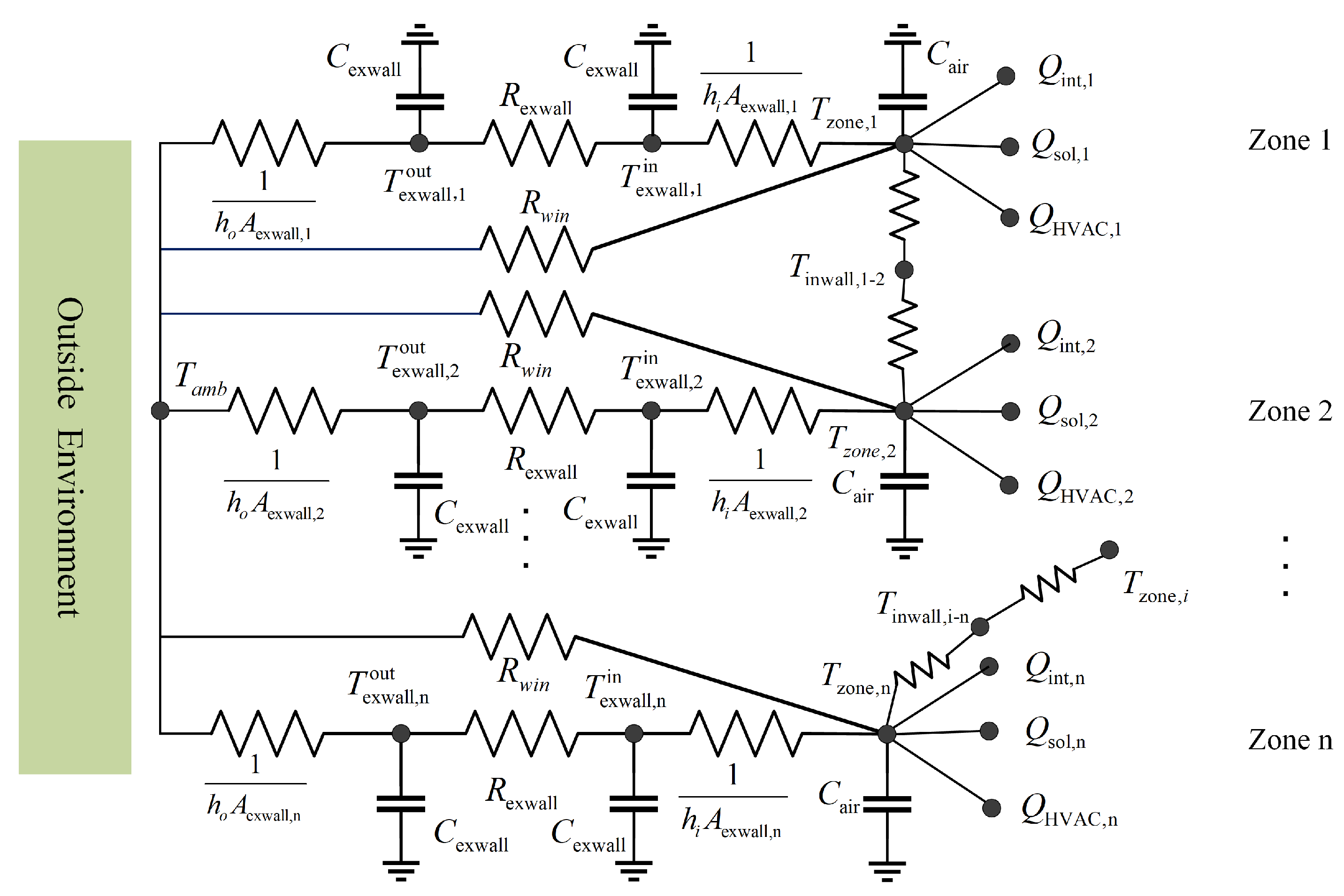
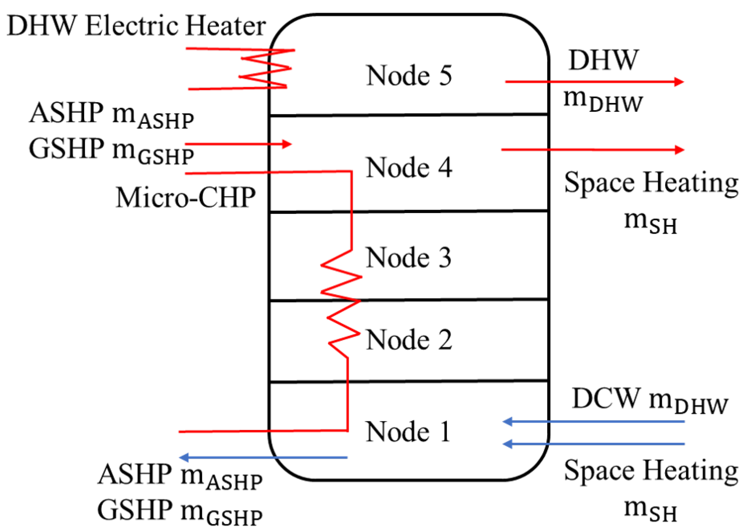
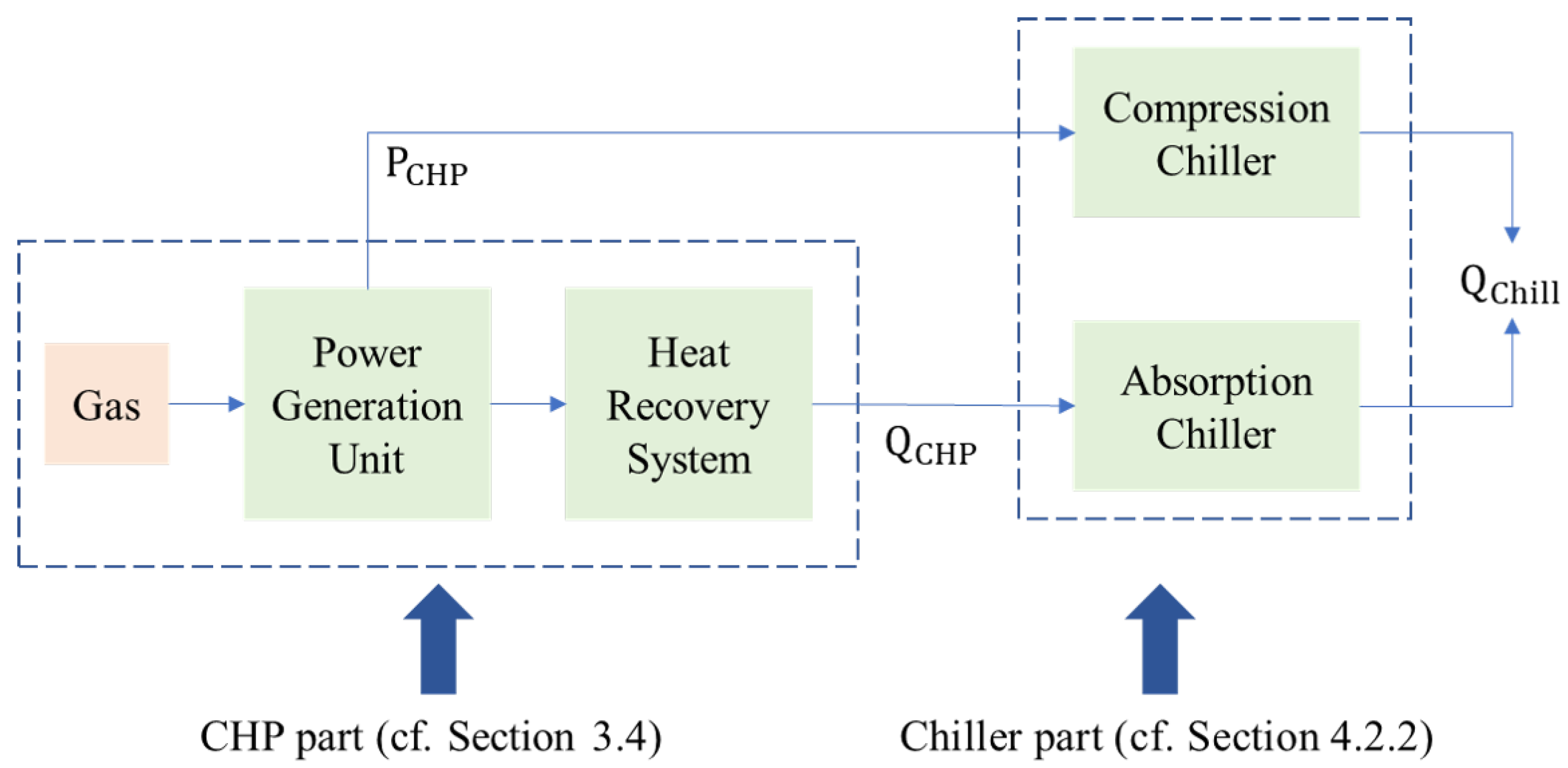
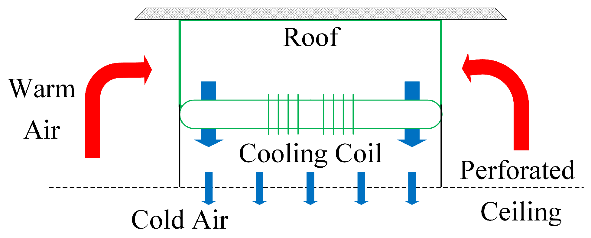
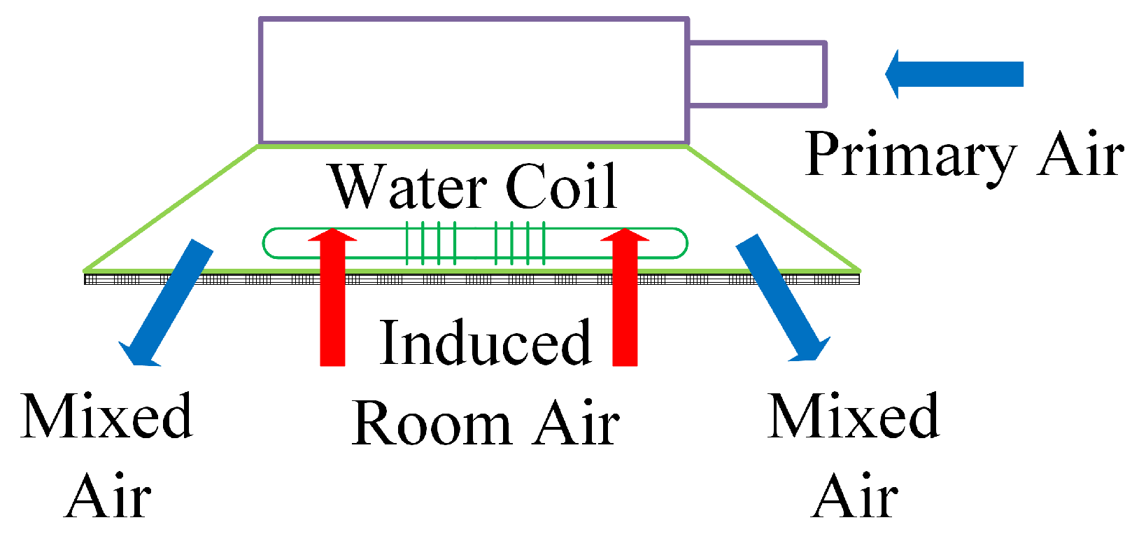
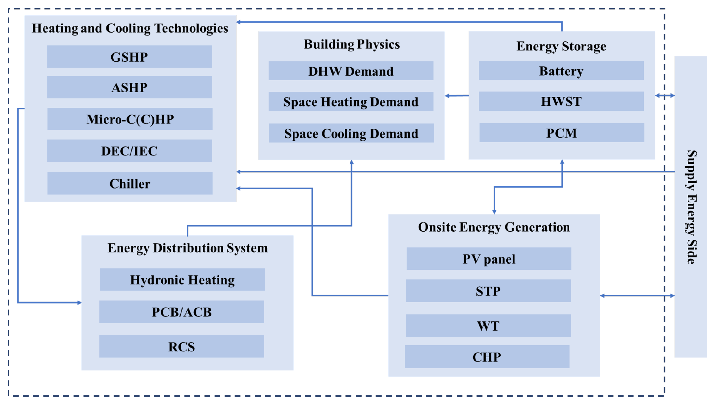
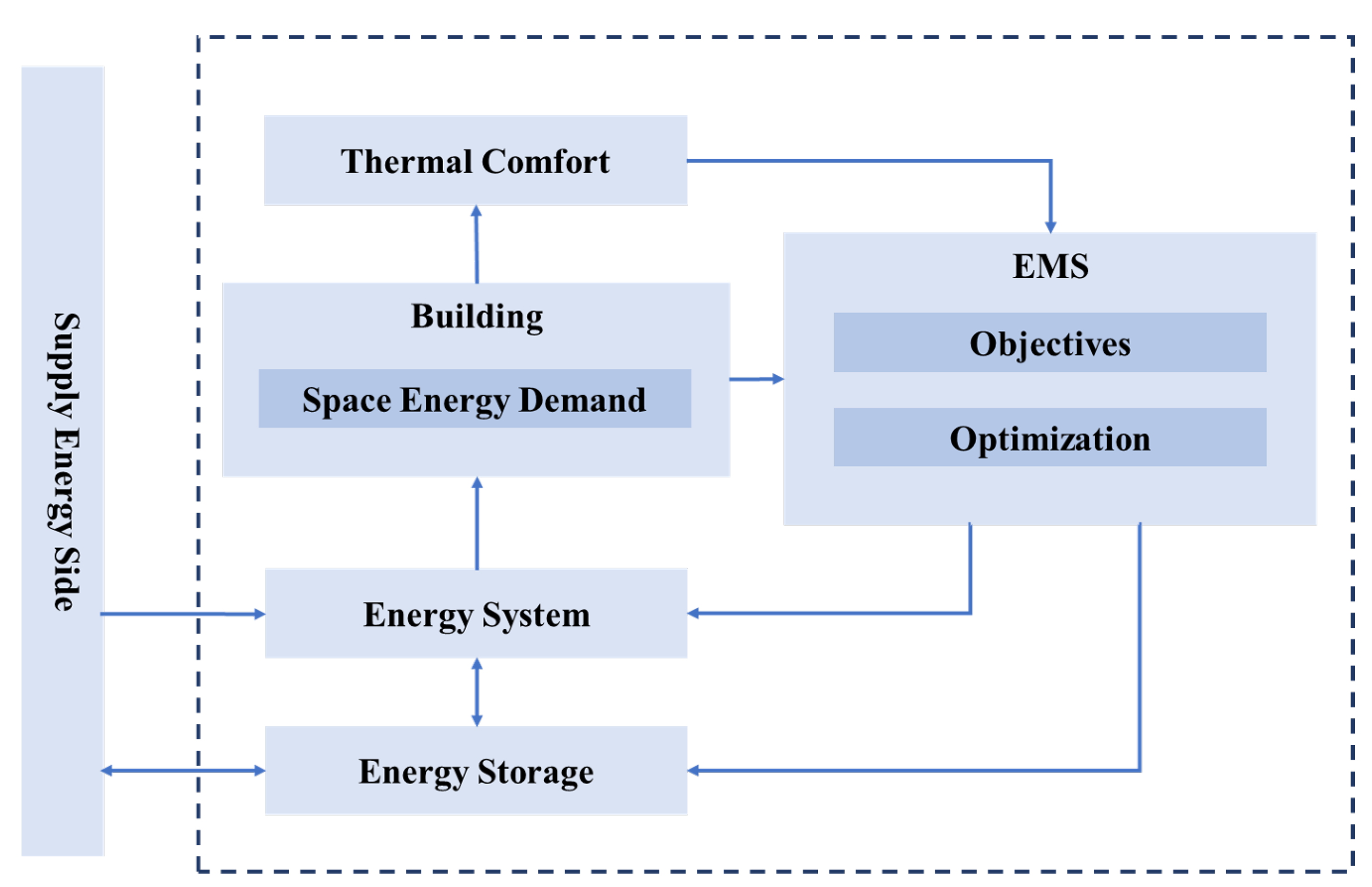
Table 1.
Studied technologies in buildings.
| Technologies | Models | Applications in Buildings | Main Findings |
|---|---|---|---|
| Photovoltaic Panel (PV) | Analytical [4] Empirical [35] | [6,36,37] | PVs can produce renewable electricity and reduce over 40% of the energy demand due to their passive benefits. |
| Solar Thermal Panel (STP) | Analytical [38] Empirical [39] | [40,41] | STPs provide renewable heat generation, with overall efficiency ranges from 24–28% (single pass) or 32–34% (double pass). |
| Wind Turbine (WT) | Analytical [5,42] Empirical [43] | [26] | WTs can produce renewable electricity and are promising in areas with strong wind currents. It grows rapidly worldwide, with an over 11% growth rate. |
| Combined (Cooling), Heating and Power (C(C)HP) | Analytical [44,45,46] Empirical [47,48] | [41,49,50] | CHP and CCHP can increase the electricity and heat production efficiency from 60% in traditional ways to 90%. |
| Battery | Analytical [36] Empirical [51] | [20,52,53] | Batteries can deal with the intermittence of renewable generation and shave peak demand, contributing to balancing the demand and supply and maintaining the grid stability, and can achieve an over 20% cost reduction. |
| Hot Water Storage Tank (HWST) | Analytical [54,55] Empirical [56] | [11,57,58] | HWSTs can shift thermal loads to off-peak hours and increase energy flexibility, providing up to a 7.5% energy saving potential and 5.5% emission reduction potential. |
| Phase Change Material (PCM) | Analytical [59,60] Empirical [61] | [62,63,64] | PCMs have large thermal storage abilities due to their high latent heat, leading to the same energy saving with less materials. |
| Air/Ground Source Heat Pump (ASHP/GSHP) | Analytical [65,66] Empirical [67,68,69] | [12,70,71,72] | Heat pumps have a high operating efficiency and low operating cost compared with conditional heating devices, with a COP of up to 5. |
| Direct/Indirect Evaporative Cooling (DEC/IEC) | Analytical [73,74] Empirical [75] | [76,77] | DEC and IEC are efficient in hot and humid climates, and can decrease the air temperature to wet bulb temperature or dew point temperature. |
| Absorption/ Compression Chiller (AC/CC) | Analytical [78] Empirical [79,80] | [81,82,83] | The COPs of chillers range from 0.6 to 6, and the consumed energy can be supplied by renewable heat/electricity production. The COP of CCs is usually higher than ACs. |
Publisher’s Note: MDPI stays neutral with regard to jurisdictional claims in published maps and institutional affiliations. |
© 2022 by the authors. Licensee MDPI, Basel, Switzerland. This article is an open access article distributed under the terms and conditions of the Creative Commons Attribution (CC BY) license (https://creativecommons.org/licenses/by/4.0/).
Share and Cite
MDPI and ACS Style
Zhang, Y.; Vand, B.; Baldi, S. A Review of Mathematical Models of Building Physics and Energy Technologies for Environmentally Friendly Integrated Energy Management Systems. Buildings 2022, 12, 238. https://doi.org/10.3390/buildings12020238
AMA Style
Zhang Y, Vand B, Baldi S. A Review of Mathematical Models of Building Physics and Energy Technologies for Environmentally Friendly Integrated Energy Management Systems. Buildings. 2022; 12(2):238. https://doi.org/10.3390/buildings12020238
Chicago/Turabian StyleZhang, Yajie, Behrang Vand, and Simone Baldi. 2022. "A Review of Mathematical Models of Building Physics and Energy Technologies for Environmentally Friendly Integrated Energy Management Systems" Buildings 12, no. 2: 238. https://doi.org/10.3390/buildings12020238
Note that from the first issue of 2016, this journal uses article numbers instead of page numbers. See further details here.