


A Variable Step Crow Search Algorithm and Its Application in Function Problems
Key Laboratory of Advanced Manufacturing and Intelligent Technology, Ministry of Education, School of Mechanical and Power Engineering, Harbin University of Science and Technology, Harbin 150080, China
*
Author to whom correspondence should be addressed.
Biomimetics 2023, 8(5), 395; https://doi.org/10.3390/biomimetics8050395
Submission received: 14 July 2023
/
Revised: 16 August 2023
/
Accepted: 24 August 2023
/
Published: 28 August 2023
(This article belongs to the Special Issue Bio-Inspired Optimization Algorithms and Designs for Engineering Applications)
Abstract
:Optimization algorithms are popular to solve different problems in many fields, and are inspired by natural principles, animal living habits, plant pollinations, chemistry principles, and physic principles. Optimization algorithm performances will directly impact on solving accuracy. The Crow Search Algorithm (CSA) is a simple and efficient algorithm inspired by the natural behaviors of crows. However, the flight length of CSA is a fixed value, which makes the algorithm fall into the local optimum, severely limiting the algorithm solving ability. To solve this problem, this paper proposes a Variable Step Crow Search Algorithm (VSCSA). The proposed algorithm uses the cosine function to enhance CSA searching abilities, which greatly improves both the solution quality of the population and the convergence speed. In the update phase, the VSCSA increases population diversities and enhances the global searching ability of the basic CSA. The experiment used 14 test functions,2017 CEC functions, and engineering application problems to compare VSCSA with different algorithms. The experiment results showed that VSCSA performs better in fitness values, iteration curves, box plots, searching paths, and the Wilcoxon test results, which indicates that VSCSA has strong competitiveness and sufficient superiority. The VSCSA has outstanding performances in various test functions and the searching accuracy has been greatly improved.
1. Introduction
The optimization is to give existing solutions and parameters to present a satisfactory answer for a certain problem. For quite some time, people have conducted large research on various optimization problems. Newton and Leibniz founded calculus which can solve some optimization problems. Then, different mathematical concepts have been proposed, such as the steepest descent method and the linear programming solution method, which can be used in many fields [1,2,3].
For specific problems, traditional methods have produced specific optimization methods for different problems. However, most of these methods have specific requirements for the searching space which requires objective functions to be convex, continuously differentiable, and differentiable. These weaknesses of traditional optimization methods are limited in solving many practical problems [4,5,6,7]. These practical production problems have large-scale, non-linear, multi-extreme values, characteristics of multiple constraints, and non-convexities, making traditional optimization methods difficult to conduct mathematical modeling. Therefore, exploring information processing methods with intelligent features is valuable.
In practical applications, intelligent algorithms generally do not require problem special information, the constraint on the problem, the continuity, the differentiability, the convexity of the objective function, and the analytical expression. Intelligent algorithms have strong adaptability to uncertainty data in the calculation process. At present, intelligence algorithms mainly include African Vultures Optimization Algorithm (AVOA) [8], Beluga Whale Optimization (BWO) [9], Whale Optimization Algorithm (WOA) [10], Flow Direction Algorithm (FDA) [11], Grey Wolf Optimizer (GWO) [12], Harris Hawks Optimizer (HHO) [13], Sine Cosine Algorithm (SCA) [14], Spotted Hyena Optimizer (SHO) [15], Slime Mould Algorithm (SMA) [16], Symbiotic Organisms Search (SOS) [17], Wild Horse Optimizer (WHO) [18], Geometric Mean Optimizer (GMO) [19], Golden Jackal Optimization algorithm (GJO) [20], Coati Optimization Algorithm (COA) [21], Dandelion Optimizer (DO) [22], Remora Optimization Algorithm (ROA) [23], Great Wall Construction Algorithm (GWCA) [24], Generalized Normal Distribution Optimization (GNDO) [25], Pelican Optimization Algorithm (POA) [26], and so on [27,28,29,30].
These algorithms have been achieved in various engineering fields [31,32,33,34,35,36]. For solving large-scale optimization problems, intelligent algorithms are significantly superior to traditional mathematical programming methods in terms of computational times and complexities.
Crow Search Algorithm (CSA) was proposed by Alireza Askarzadeh in 2016 [37]. Crows will hide their food and remember its hiding location for several months. At the same time, they will track other crows to steal food. Based on the living habits of crows in nature, the crow search algorithm has been proposed. From the algorithmic perspective, the overall flying area of the crow population is the searching space. The position of each crow represents the algorithm feasible solution and the location of crow hidden food represents the algorithm’s objective function value. The best food position in the algorithm is the optimal solution in the searching space.
Shalini Shekhawat and Akash Saxena designed the Intelligent Crow Search Algorithm (ICSA) and used ICSA in the structural design problem, frequency wave synthesis problem, and Model Order Reduction [38]. Yilin Chen et al. introduced a robust adaptive hierarchical learning Crow Search Algorithm for feature selection [39]. Primitivo Díaz et al. introduced an improved Crow Search Algorithm Applied to Energy Problems [40]. Amrit Kaur Bhullar et al. proposed the enhanced crow search algorithm for AVR optimization [41]. Thippa Reddy Gadekallu et al. used CNN-CNS for handing gesture classification [42]. Malik Braik et al. designed a hybrid crow search algorithm for solving numerical and constrained global optimization problems [43]. Behrouz Samieiyan et al. applied Promoted Crow Search Algorithm (PCSA) to solve dimension reduction problems [44]. Qingbiao Guo et al. used an improved crow search algorithm for the parameter inversion of the probability integral method [45]. CSA has been applied in many fields.
In the basic CSA, crows update their positions by the fixed flight length in the searching space, wherein the fixed flight length will make the individual jump out of the fitness solution region, which can cause low searching accuracy. As a result, this paper proposes a variable step crow search algorithm (VSCSA). VSCSA uses Cosine function steps to update its positions. The rest of this paper is organized as follows: In Section 2, this paper gives the basic CSA. In Section 3, this paper proposes VSCSA. In Section 4, the function experiment results analysis is shown. In Section 5, the CEC2017 function experiment results analysis is shown. In Section 6, engineering application problems are shown. In Section 7, the conclusion is given.
2. Crow Search Algorithm
The crow is the general name of passerine corvus that is a large songbird which has a sturdy mouth and feet. Nostrils are circular and usually covered by feather whiskers. Crows like to live in groups and have strong clustering. They are forest and grassland birds with a steady gait. Except for a few species, they often gather in groups and nest, and wander in mixed groups during the autumn and winter seasons, flying and singing. Generally, the personality is fierce and full of aggressive habits. CSA is a metaheuristic algorithm based on crow intelligent behaviors. Crows will steal food by observing where the other birds hide their food, if a crow finds the thief, it will move to hiding places to avoid being a future victim. And crows use their own experiences to predict the pilferer’s behavior. In CSA, the crow overall flight area is the searching space, and the position of each crow gives a feasible solution. The crow hidden food represents the quality of the algorithm function value.
The CSA Step is given in this section.
Step 1: Initialize the problem and adjustable parameters.
Set CSA size N, the maximum number of iterations itermax, the flight length (fl), the awareness probability AP, and the searching dimension is d. The crow i at one iteration in the searching space is specified by a vector xi,iter(i = 1, …, N; iter = 1, …, itermax). The searching upper bound is ubi(i = 1, …, N) and the searching lower bound is lbi(i = 1, …, N),
Step 2: Initialize position and memory.
Each crow will save its hidden food location m during each iteration, which represents the best position the crow currently has because during the initial iteration of the algorithm, the crow is inexperienced. Therefore, the initial memory, which is the location where the crow first hides its food, is set as their initial position.
Step 3: Evaluate the objective function.
Compute one crow position.
Step 4: Generate a new position.
Crow i will generate a new position. In this case, two states will happen:
State 1: Crow i will approach crow j.
State 2: Crow j will go to another position.
States 1 and 2 can be expressed as follows:
where ri is a random number in the range of [0, 1] and fli;iter denotes the flight length of crow i at iteration iter. AP denotes the awareness probability.
Step 5: Check the feasibility of new positions.
Check the new position feasibility of each crow.
Step 6: Evaluate fitness functions of new positions.
Calculate all feasible solutions. The function value for the new position of each crow will be calculated.
Step 7: Update memory
The crows update their memory as follows:
Compare all fitness function values. If there is a better fitness function value of the new position, the memory will be updated.
Step 8: Check termination criterion.
Calculate iter = iter + 1. Stop if the termination criterion is met iter = itermax. If not, Steps 4–7 are repeated until the itermax is reached.
3. Variable Step Crow Search Algorithm
In the original CSA, crows constantly update their positions in the searching space, but their flight length fl is fixed, and the solutions to the search problem are diverse. When initializing a population, individuals often cannot directly locate the optimal solution and approach the region where the optimal solution is located without prior exploration experience in the searching space as a guide. Therefore, the searching process should be carried out in multiple different directions to expand the searching scope and thereby increase the probability of approaching the area. In addition, individuals in the population often wish to visit unexplored areas when exploring the searching space, thereby increasing the breadth of the search. And from the CSA position update formula, it can be seen that the crow population mainly updates its position by moving towards a fixed flight length. Therefore, as the species iteration continues, the crow population will gradually cluster and the population diversity will gradually decrease, which can easily lead to a single searching direction and form too many local optima which is not conducive to the algorithm’s small-scale search in the later stage. To solve this problem, this article proposes a variable step crow search algorithm (VSCSA).
The cosine function is a Periodic function with a minimum positive period of 2π. When the independent variable is an integer 2kπ (k is an integer), the function has a maximum value of 1. When the independent variable is (2k + 1) π (k is an integer), the function has a minimum value of −1. The cosine function is an even function, and its image is symmetric about the y-axis.
When crow j knows that crow i is following it, then as a result, crow j will go to another position by the searching upper bound.
New states 1 and 2 can be expressed as follows:
where rsi is a random number in the range of [−1, 1] and ubi(i = 1, …, N) is the searching upper bound.
VSCSA improves the population diversity and the changing pattern search guidance method during the evolution process. In the early searching stage, the population diversity is relatively high. Cosine steps serve as a guide for population evolution, which can avoid blind individual searching and population diversity rapid decay. This meets the requirement that the algorithm should conduct a large-scale exploration as much as possible during the initial iteration. In the later searching stages, the proposed algorithm will shift from a global exploration to a local development, which can avoid the divergence in search directions. When the population falls into the local optima, the proposed algorithm can use individuals generated by cosine steps as searching guides to effectively increase population diversities and jump out of different local optima areas. Therefore, the proposed strategy reflects the adaptive interaction between population diversities and multiple search guided individuals, the changes in the population searching steps reflect different stages of evolution, and different searching guided methods can be adaptively selected. In turn, different guided methods can alter the diversity of the population, expand the algorithm searching range, and strengthen the algorithm searching precision.
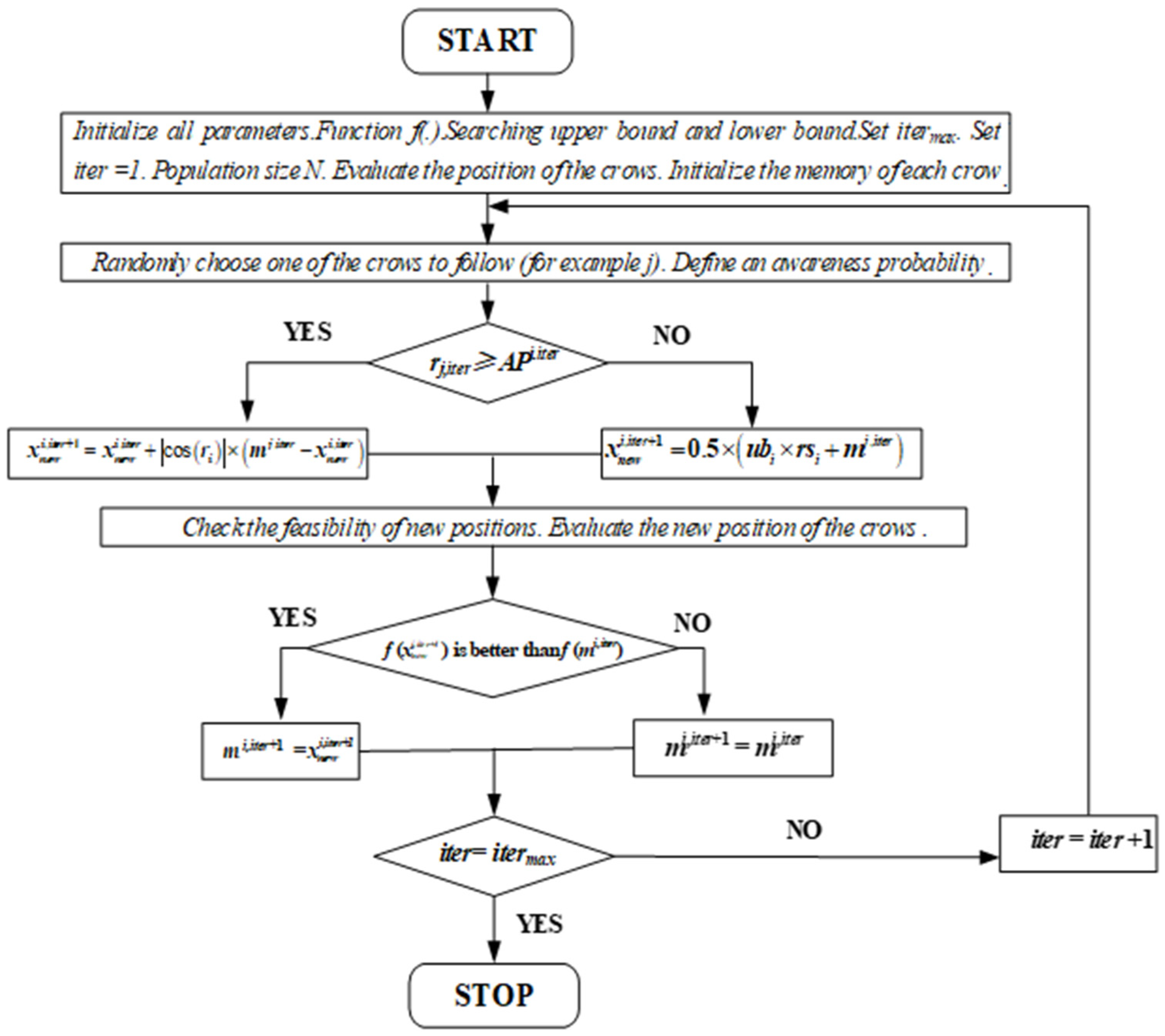
The VSCSA Flowchart can be presented in Figure 1 as follows:
The VSCSA pseudo code can be summarized in Algorithm 1.
| Algorithm 1: VSCSA. |
| Input: Function f(.). Searching upper bound and lower bound. Set itermax. Set iter = 1. Population size N. Evaluate the position of the crows. Initialize the memory of each crow. While (iter < itermax) For i = 1:N Randomly choose one of the crows to follow (for example j). Define an awareness probability. If 1 rj,iter≥ APi.iter = + |cos(ri)| × (mj,iter − ) Else = 0.5 × (ubi × rsi + mj,iter) End If 1 End For Check the feasibility of new positions. Evaluate the new position of the crows. Update the memory of crows: If 2 f () is better than f (mi,iter). mi,iter+1 = Else mi,iter+1 = mi,iter End If 2 iter = iter + 1 End While |
4. Function Experiment Results
4.1. Experiment Environments
Different functions are in Table 1. In Table 1, D is the searching dimension and fmin is the idea function value. Range is the searching scope. Different optimal solutions of high-dimensional testing functions in this paper are hidden in a smooth and narrow parabolic valley, with broad searching space, tall obstacles, and a large number of local minimum points. This paper uses different test functions for comparing VSCSA and standard CSA performances. This paper tests VSCSA with the cuckoo search algorithm (CS) [46], the sine cosine algorithm (SCA) [14], and the moth-flame optimization algorithm (MFO) [47]. CS was proposed by Xin-She Yang and was inspired by the cuckoo incubation mechanism in nature. The size of the cuckoo bird is similar to that of a pigeon, but it is slender and has a dark gray upper body. SCA, which was proposed by Seyedali Mirjalili in 2016, was inspired by sine and cosine mathematical terminology. MFO, which was proposed by Seyedali Mirjalili in 2015, was inspired by the moth navigation in nature called the transverse orientation. In this chapter, the CS discovery probability was set as 0.25 and the step was set as 0.25. For SCA, a = 2, r2 = 2π, r3, and r4 were selected in [0, 1]. In CSA, fl = 2. All algorithm parameters were selected from the original algorithm literature. The population size was 20, the maximum iterations were 400, and it was ran 10 times in MATLAB (R2016b).
4.2. Data Results
In Table 2 and Table 3, Min, Max, Ave, and Var mean the minimum value, the maximum value, the average value, and the variance deviation. Table 2 shows two-dimension function results. Table 3 shows high-dimension functions results. For two-dimension functions, VSCSA can obtain the ideal function values in f2 to f5, f12(D=2), and f13(D=2). And VSCSA can obtain the ideal values of all evaluation indexes in f2 to f4. CSA can obtain ideal function values in f12(D=2), f13(D=2). MFO can obtain the ideal function values in f2 to f5, f12(D=2), and f13(D=2). MFO can obtain the ideal values of all evaluation indexes in f2, f3, f5. SCA can obtain the ideal function values in f2 to f4, f12(D=2), and f13(D=2). SCA can obtain the ideal values of all evaluation indexes in f2 to f4. Min values of MFO in f10 and f14(D=2) are better than those of VSCSA. Min value of SCA in f14(D=2) is better than that of VSCSA. For high dimension functions, the Min values of SCA in f11(D=30), f12(D=60), f13(D=60), f13(D=200) are better than those of VSCSA. Min value of MFO in f12(D=30) is better than that of VSCSA. VSCSA in other results are all less than comparative algorithms. VSCSA can ensure continuous evolution and has good convergence speed and optimization accuracy. Especially for multi-peak high dimension functions with rotational characteristics, the proposed algorithm can better overcome the interference caused by local extreme points in the solving process, can prevent premature convergence, ensure continuous population evolution, and ultimately achieve a high optimization accuracy.
4.3. Iteration Results
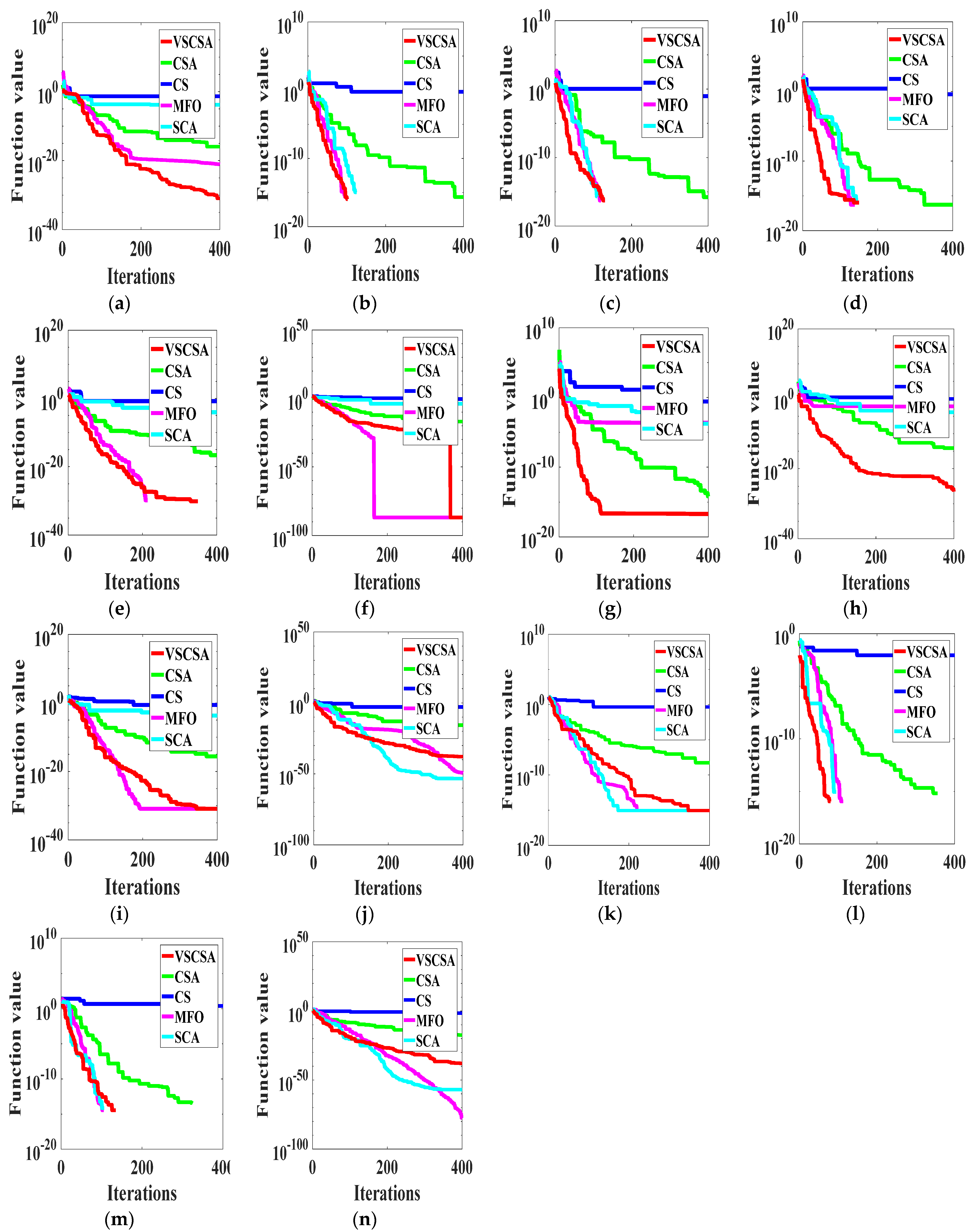
This paper gave algorithm optimal iteration curves after 10 independent operations, as shown in Figure 2 and Figure 3. Compared with different algorithms in two-dimension iteration curves, VSCSA has the fastest iteration curve except for f10, f13(D=2), f14(D=2). In f10, SCA has the fastest iteration curve. In f13(D=2), f14(D=2), MFO has the fastest iteration curve, and CSA has the second fast iteration curve. Compared with different algorithms in high-dimension iteration curves, VSCSA has the fastest iteration curve except f11(D=30), f12(D=30), f12(D=60), f13(D=60). In f11(D=30), f12(D=30), f12(D=60), f13(D=60), SCA has the fastest iteration curve. The VSCSA has outstanding performances in various test functions, whereby especially the searching accuracy has been greatly improved. Therefore, the iteration curve can display that VSCSA has a strong searching performance.
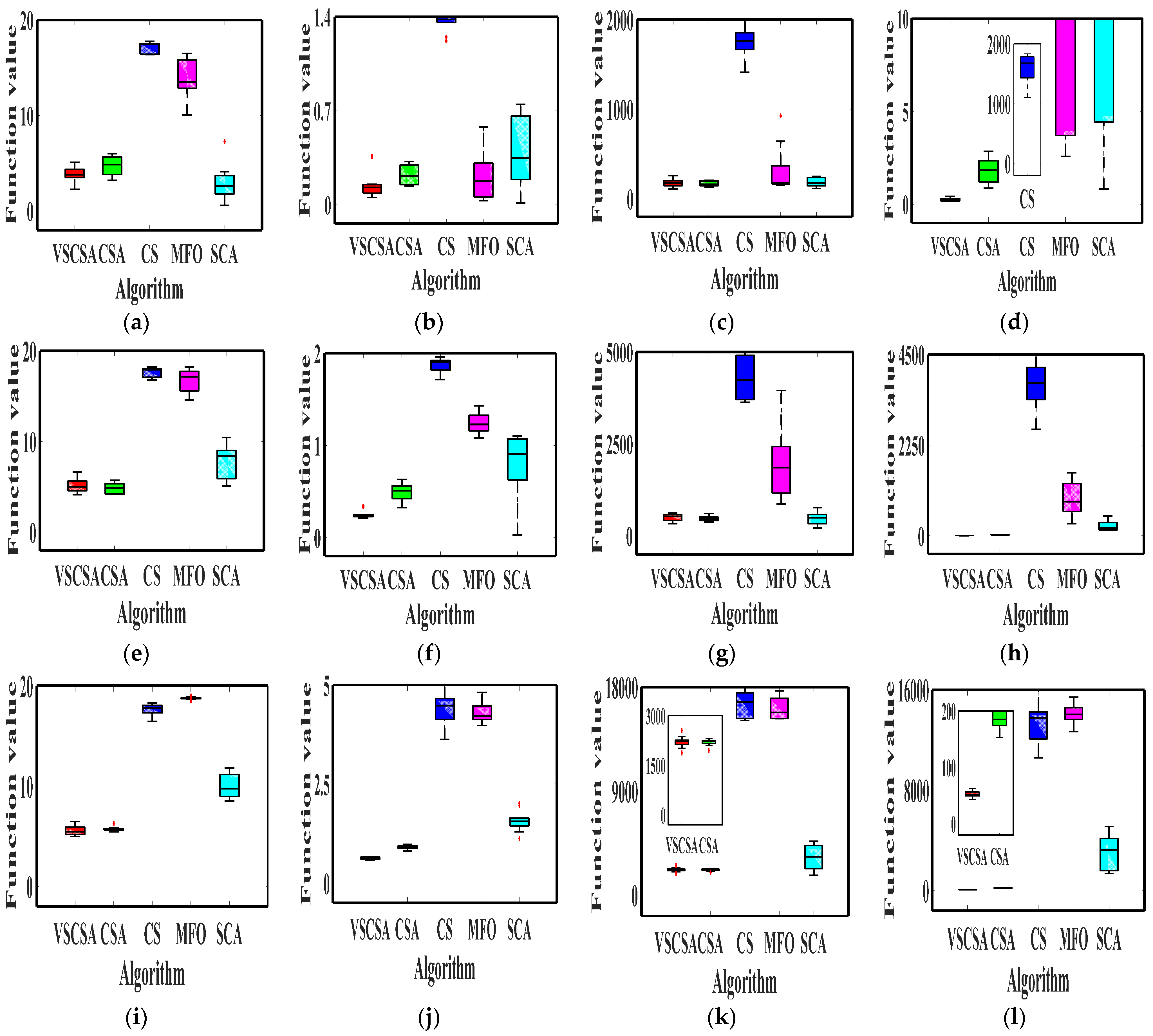
4.4. Box Plot Results
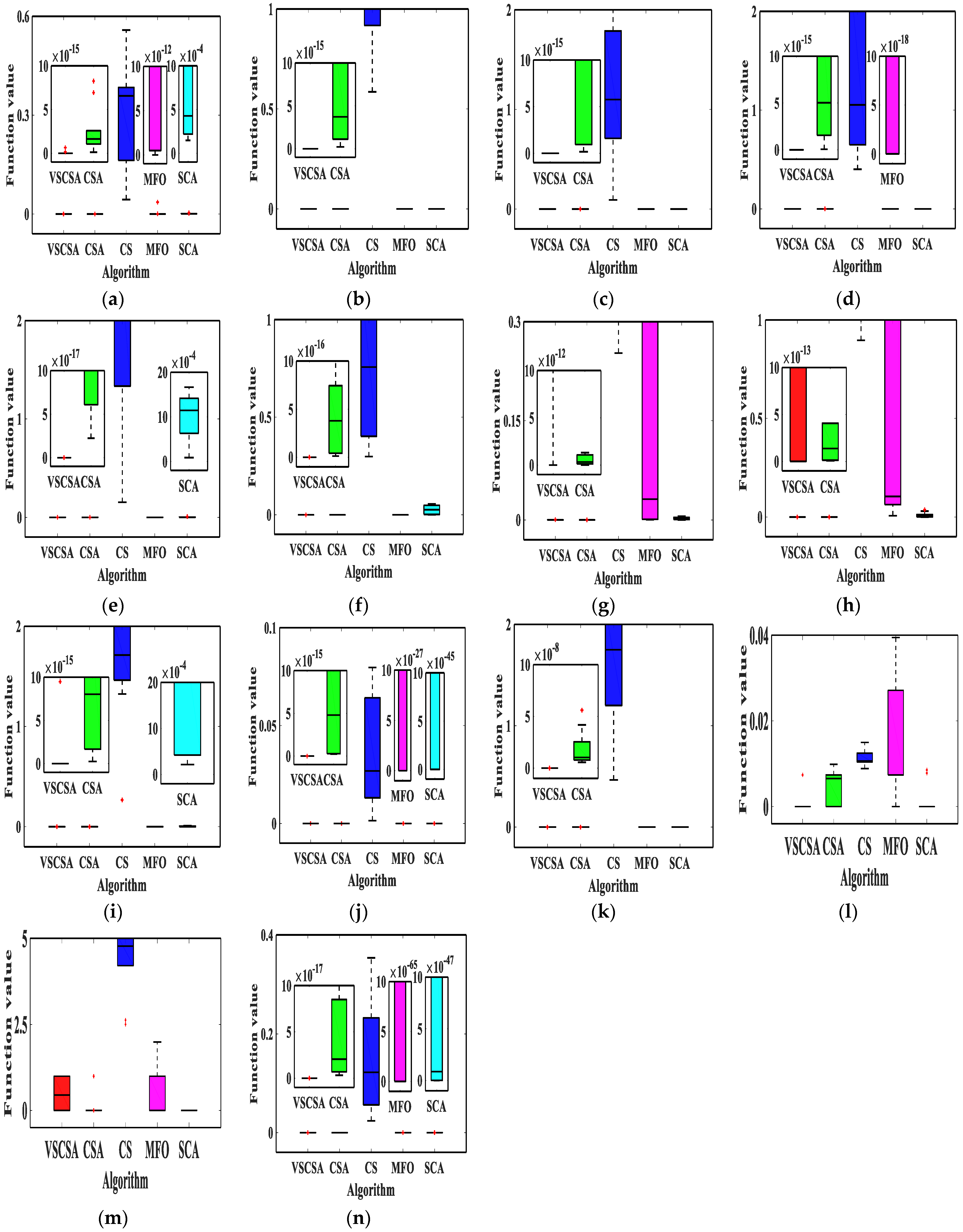
The box plot connects the two quartiles and connects the upper and lower edges to draw the box plot, and the median is in the middle of the box plot. If the box plot is narrower, the data is more concentrated. This paper gave algorithm box plots, as shown in Figure 4 and Figure 5. Compared with different algorithms in low-dimension box plots, VSCSA has the narrowest box plot except for f8, f13. In f8 and f13, CSA has the narrowest box plot. Compared with different algorithms in high-dimension box plots, VSCSA has the narrowest box plot except for f11(D=60), f13(D=60), f11(D=200), f13(D=200). In f11(D=60), f13(D=60), f11(D=200), f13(D=200), CSA has the narrowest box plot. Compared to the standard CSA algorithm, the VSCSA algorithm not only has a higher solving accuracy but also runs faster in most testing functions, which fully demonstrates that the VSCSA retains outstanding local search ability and is a significant improvement in global searching performances.
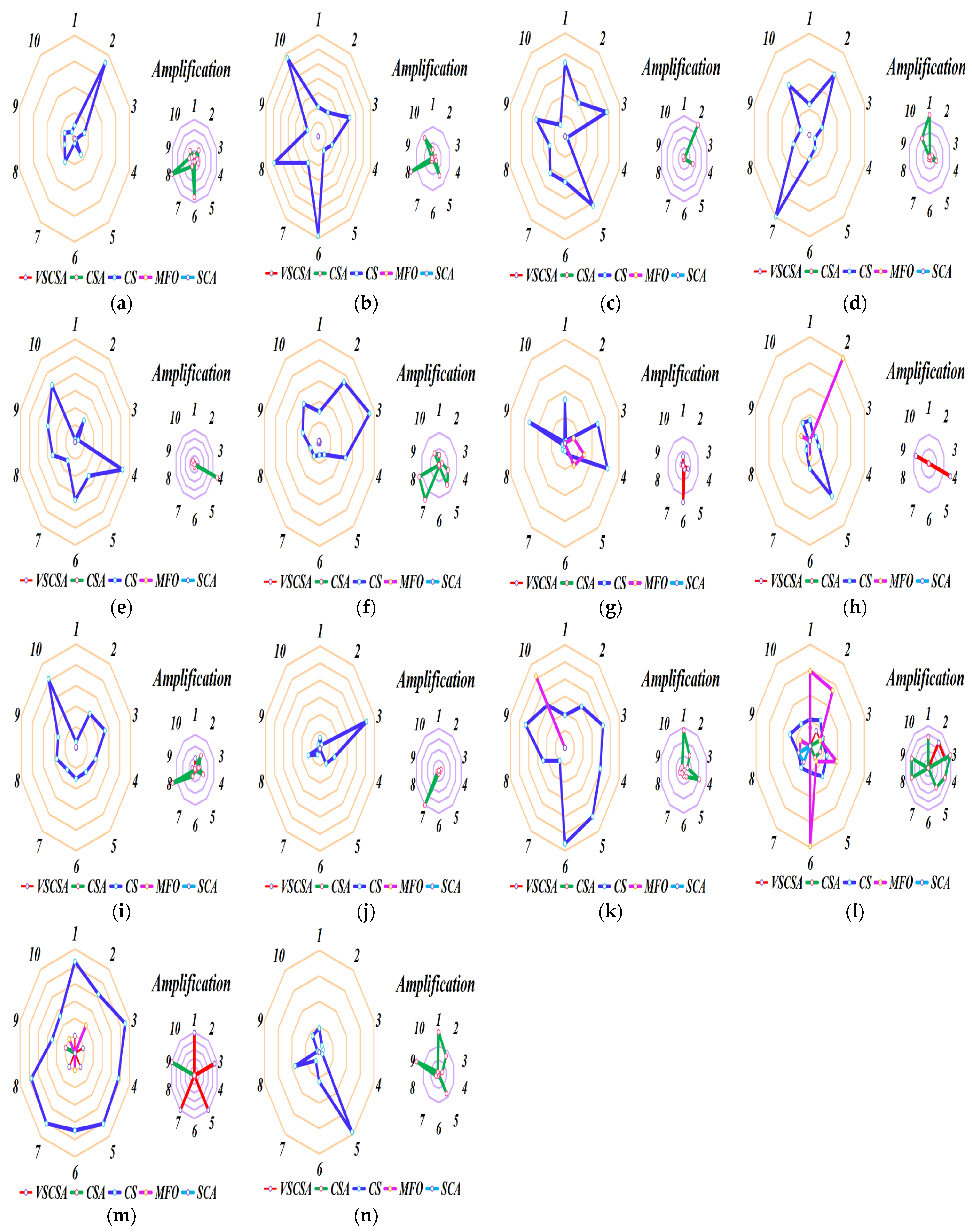
4.5. Sub-Sequence Runs Results
Different axes are projected at equal angular intervals from the same center point, each axis represents a quantitative variable, and points on each axis are sequentially connected into lines or geometric shapes. Each variable has its axis, with equal distances between them, and all axes have the same scale. It is equivalent to a parallel coordinate map, which is arranged radially along the axis. This paper shows the basic statistical assessment obtained in sub-sequence runs of different algorithms. Ten sub-sequence runs are shown in Figure 6 and Figure 7. If the total length of polygon edges with different colors is longer, the lower the accuracy of the algorithm subsequence operations. For two-dimension amplification radar charts, CS subsequences have the largest radar charts except for f12(D=2). MFO radar charts are larger than CSA radar charts in f12(D=2). For high-dimension amplification radar charts, CS subsequences have the largest radar charts except for f11(D=60), f11(D=200) to f14(D=200).
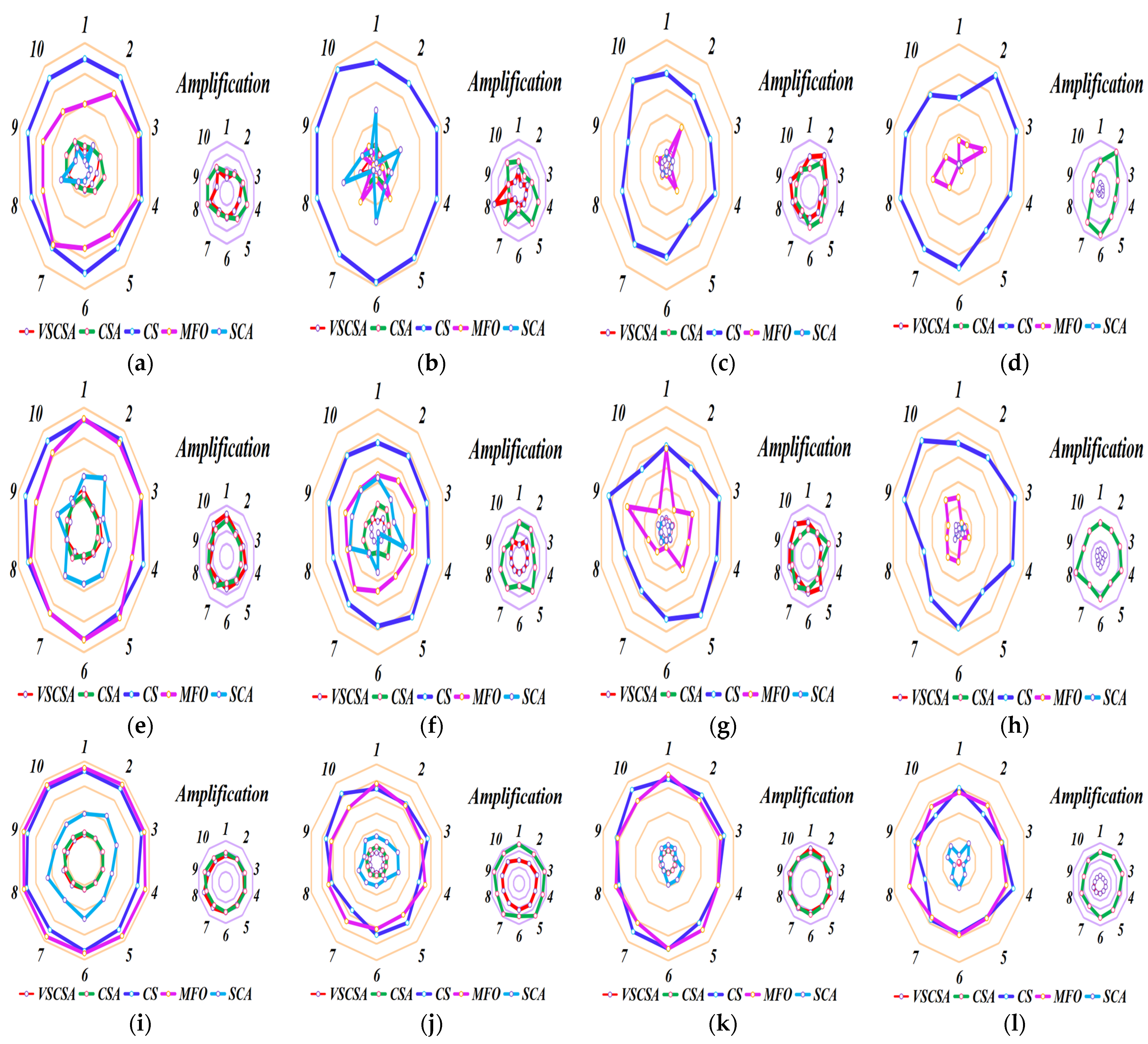
4.6. Search Path Results
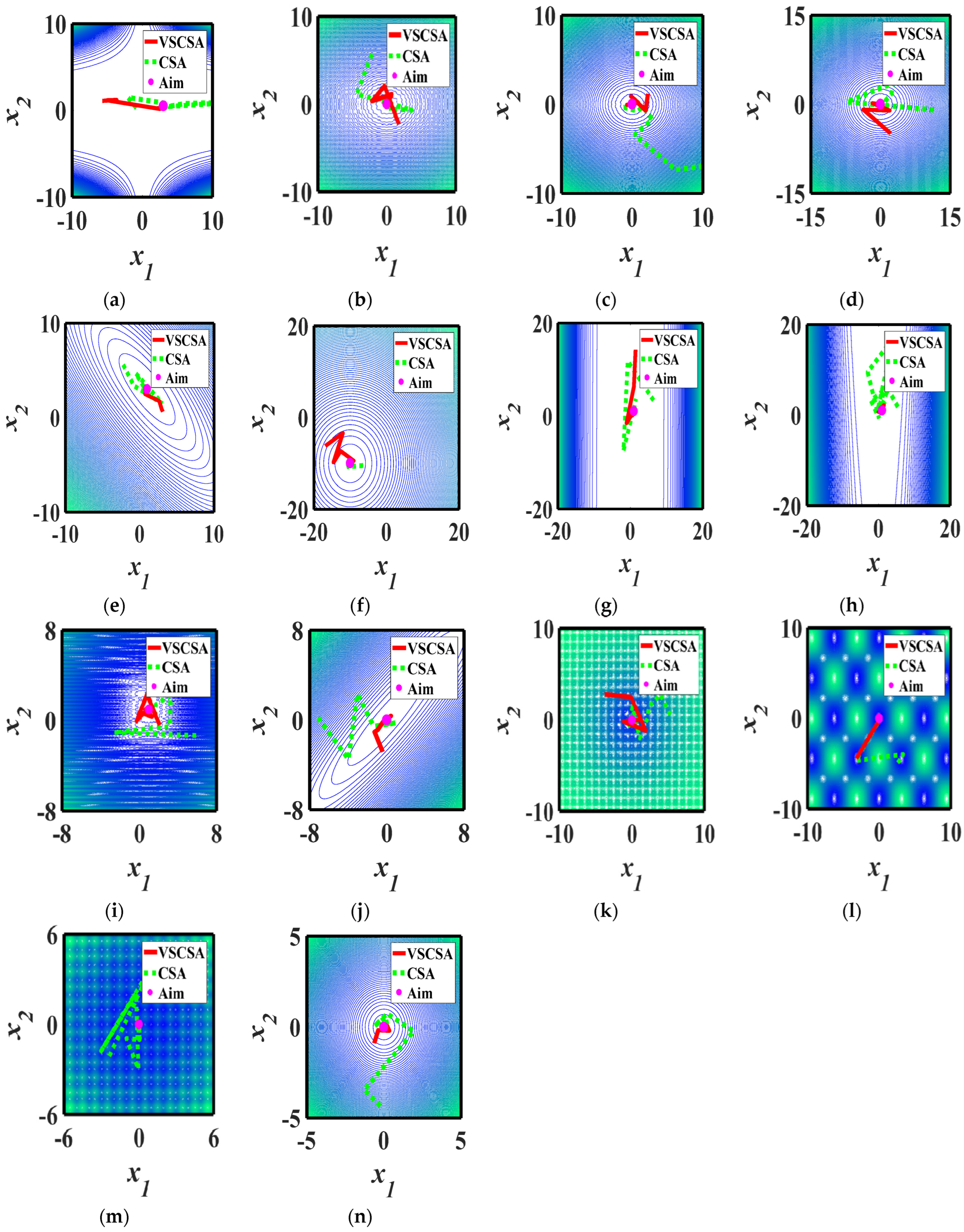
To test the structural reliability analysis, the computational efficiency, and the accuracy of the proposed algorithm, three-dimensional images of two-dimension functions are given in Figure 8, while the VSCSA path and the CSA path are refracted to a two-dimension plane in Figure 9. The red straight line is the VSCSA searching path, the green dashed line is the CSA searching path, and the pink dot is the theoretical optimal position. CSA searching paths have many short repeat searching paths and occasional long searching paths. The VSCSA algorithm has a strong performance in population diversity, representing the global optimal performance. In the early stage of the algorithm searching process, the VSCSA can quickly traverse and explore the entire solution region, lock in the approximate range of the global optimal solution, and ensure the diversity of the population. At the end stage of the algorithm searching process, the reduction of differences between individuals makes the searching process jump out of local vortices and find the ideal optimization solution, which can improve the algorithm global convergence ability.
4.7. Wilcoxon Rank Sum Test Results
In the process of detecting algorithms, more different experimental results often appear. When comparing and analyzing algorithms, conclusions cannot be drawn solely based on differences in a few results, so statistical analysis should be conducted to test the significance of differences in the data. The Wilcoxon rank sum test result is the p-value. If the p-value is greater than 0.05, there is no significant change for two sets of data. If the p-value is less than 0.05, two algorithm performances are significant. In Table 4, N means that the computer cannot give the p-value because of the too-large or too-small p-value. In function f8, f13(D=2), f11(D=30), f13(D=30), f11(D=60), f13(D=60), f11(D=200), f13(D=200), the p-value in CSA is larger than 0.05. In function f4, f10, f11(D=2), f13(D=2), f12(D=30), f13(D=30), the p-value in MFO is larger than 0.05. In function f11(D=2), f12(D=2), f11(D=30), f13(D=30), f13(D=60), the p-value in SCA is larger than 0.05. For other algorithms, the Wilcoxon rank sum test results are all less than 0.05. From the results of the Wilcoxon rank sum test by VSCSA, the searching accuracy of the algorithm has been significantly improved, and the improved algorithm is significantly better than the standard CSA in terms of searching accuracy and speed.
4.8. Algorithm Ranking Results
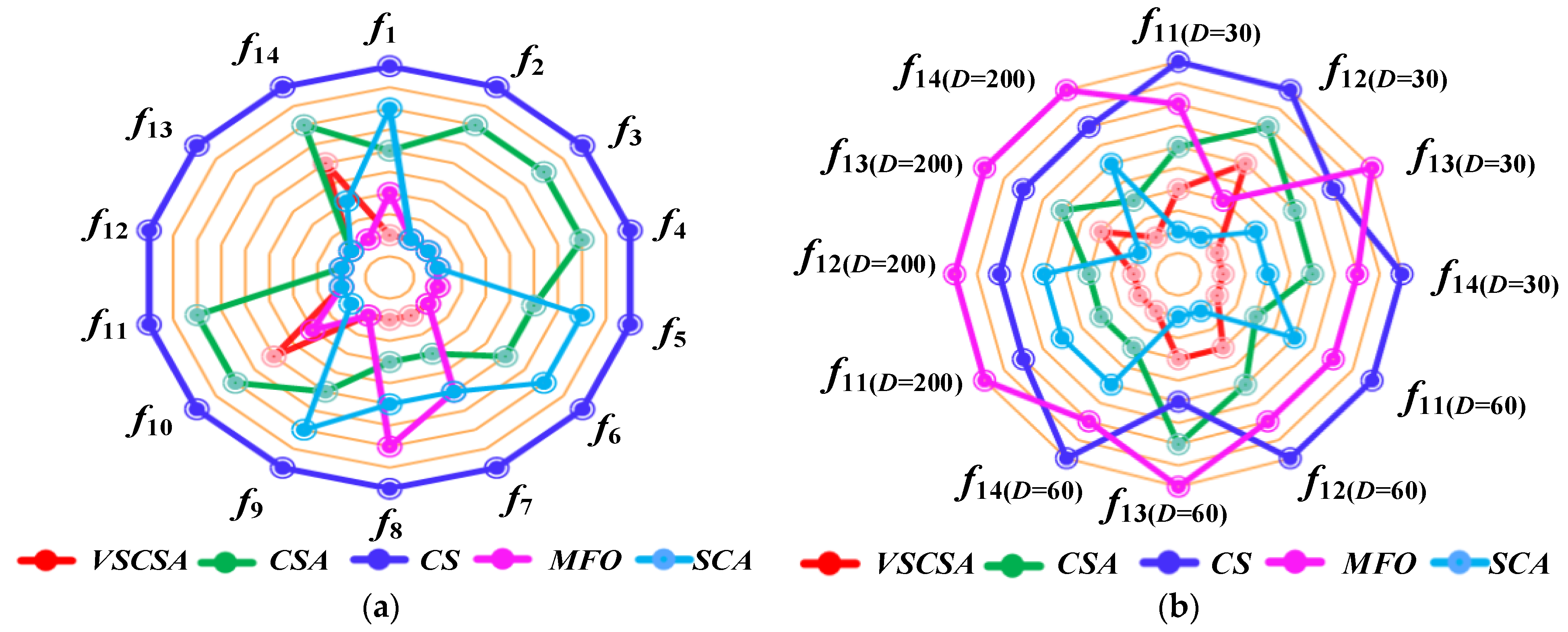
Algorithm ranking radar charts are shown in Figure 10. The positions of different colored dots in the radar image represent the algorithm searching accuracy. If the algorithm point is close to the center point, the algorithm has a high ranking. It can be seen that the VSCSA surrounds the center point. From the radar graph, it can be seen that VSCSA has the best results among multiple test functions and has the highest searching accuracy among comparison algorithms. Although VSCSA did not achieve comprehensive advantages in some test functions, it achieved optimal searching results in more than half of the test functions, indicating that VSCSA has strong competitiveness. It can be seen that the proposed VSCSA in this paper greatly enhances the CSA searching performance.
5. CEC2017 Test Function Experiment Results
5.1. Experiment Environments
The IEEE Congress on Evolutionary Computation (CEC) is one of the largest and most significant conferences within Evolutionary Computation (EC). CEC test functions under the CEC conference series are among the widely used benchmarks to test different algorithms. CEC2017 is the test function in the 2017 CEC conference. CEC2017 consists of different problems, including Unimodal, Multimodal, Hybrid, and Composition functions. To further show the proposed algorithm, this paper selected CEC2017 in F1 to F20. F1 to F20 of CEC2017 are given in Table 5. In Table 5, D is the searching dimension, Fmin is the idea function value, and range is the searching scope. F1 and F2 are Unimodal Functions, F3 to F9 are Simple Multimodal Functions, F10 to F19 are Hybrid Functions, and F20 is the Composition. In this paper, the proposed method compares with state-of-the-art algorithms (SOTA) in recent years. SOTA includes the bald eagle search algorithm (BES) [48], COOT bird algorithm (COOT) [49], wild horse optimizer (WHO) [18], and whale optimization algorithm (WOA) [10]. All algorithm parameters were selected according to original literature. The population size and the maximum number of iterations were 20 and 5000, respectively. To obtain a fair comparison result, all algorithms independently ran 10 times in MATLAB(R2016b). The experimental environment was the Windows 7 operating system, Intel (R) Core (TM) i3-7100CPU, 8GBRAM.
5.2. Experiment Results
The statistical results of algorithms on CEC2017 benchmark functions are shown in Table 6. In Table 6, Min, Max, and Var mean the minimum value, the maximum value, and the variance deviation. For Unimodal Functions, VSCSA, CSA, BES, COOT, and WHO can obtain the ideal value in F1. All six algorithms can obtain the ideal value in F2. For Simple Multimodal Functions, all six algorithms can obtain the ideal value in F3 to F9. For Hybrid Functions, all six algorithms can obtain the ideal value in F10 and F11. CSA can obtain the minimum value in F12. BES can obtain the minimum value in F17. COOT can obtain the minimum value in F14 F16. WHO can obtain the minimum value in F13 F15 F18 F19. For the Composition, COOT can obtain the minimum value in F20.
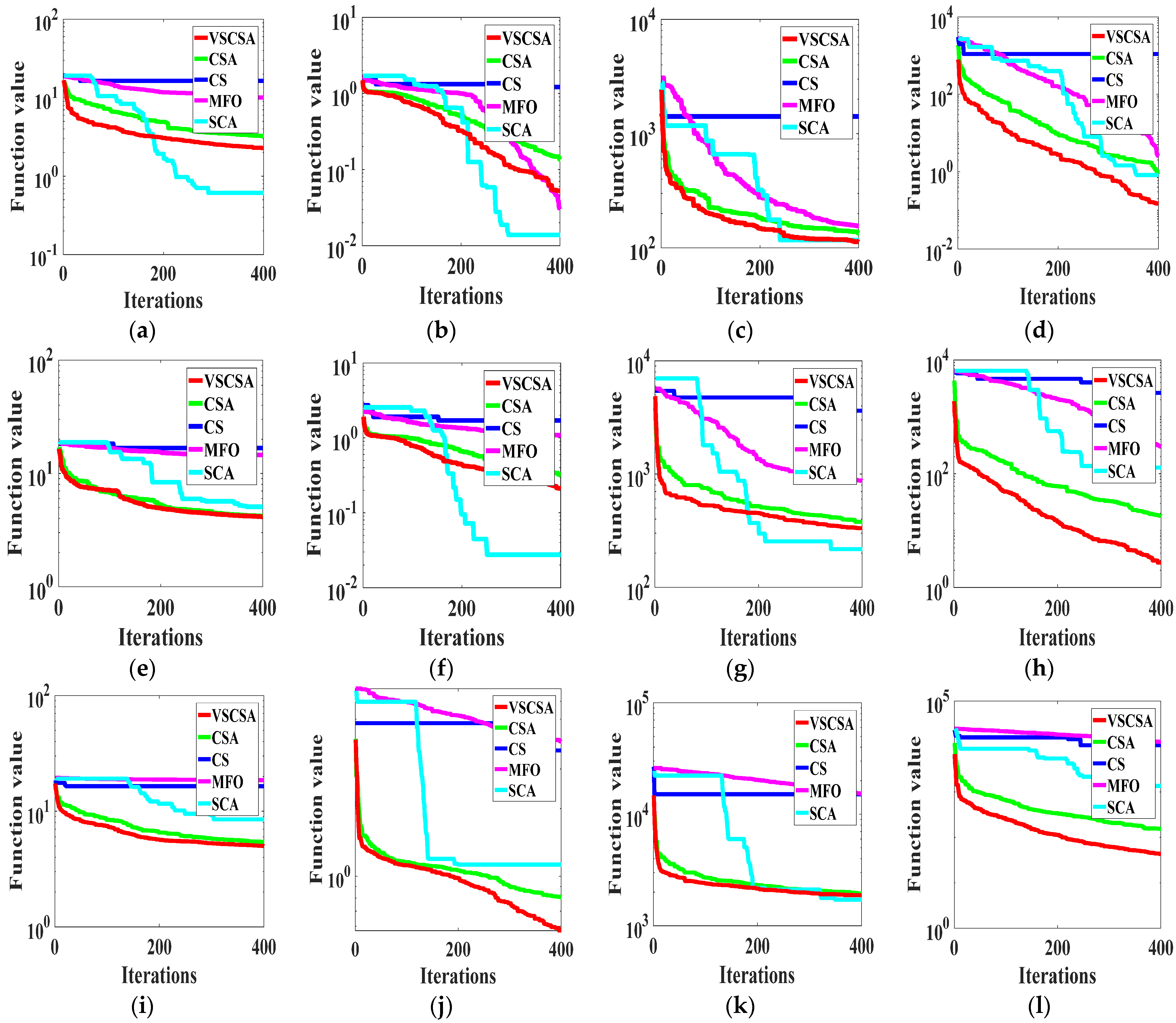
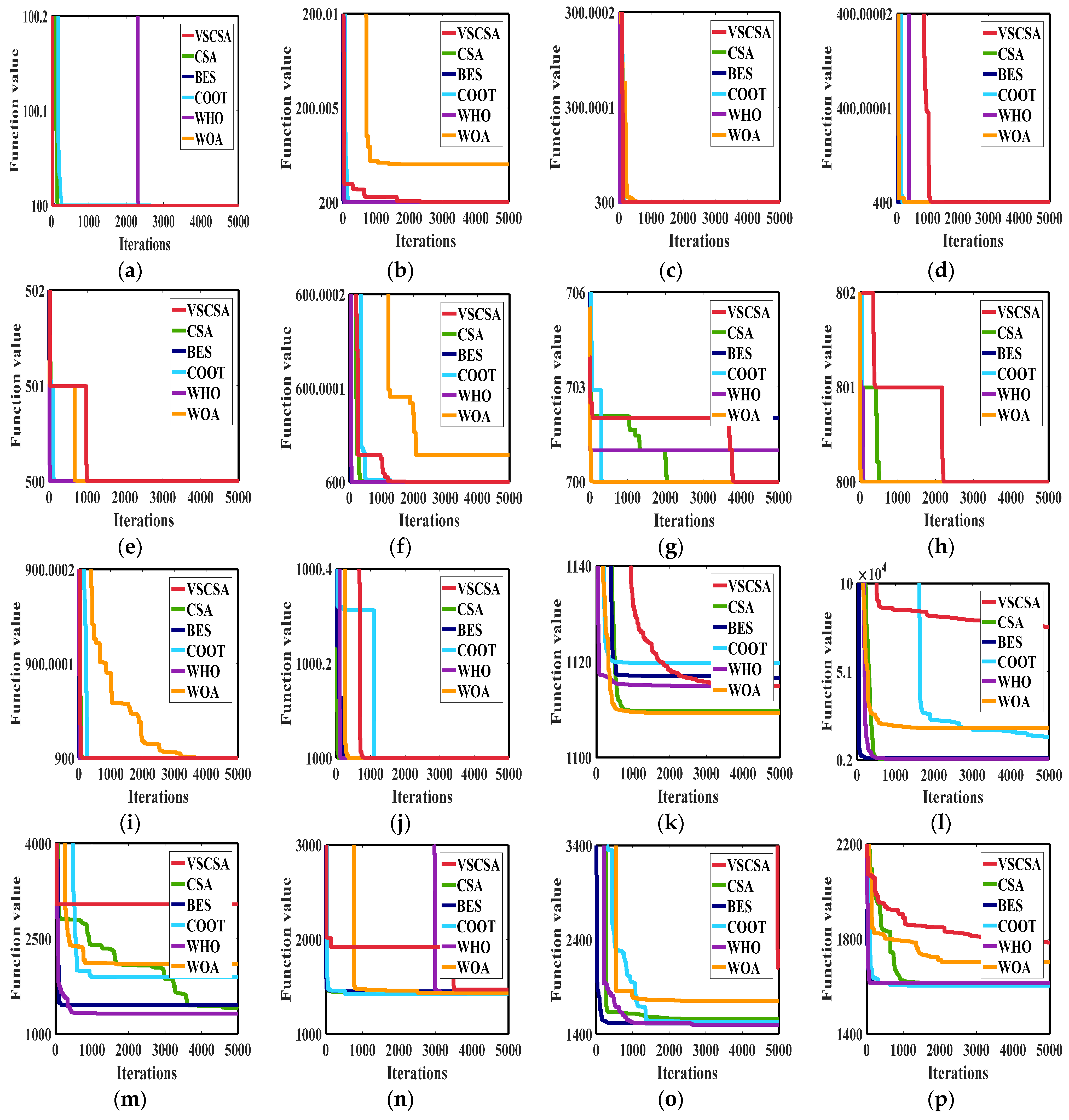
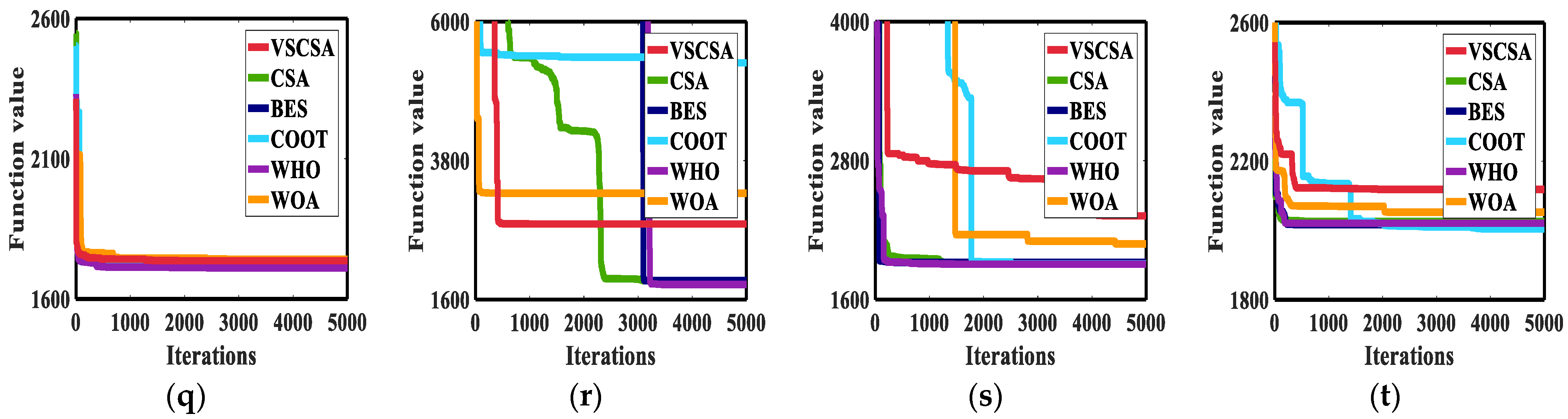
Figure 11 gives the best iteration curves of different algorithms in 10 independent runs. From Figure 11 we can see that VSCSA has the fastest initial iteration speed in function F1, F3, and F9. And VSCSA has the fastest iteration speed in the later stage for function F2, F4 to F8, and F10. VSCSA has the slowest iteration speed in F12, F15, and F16.
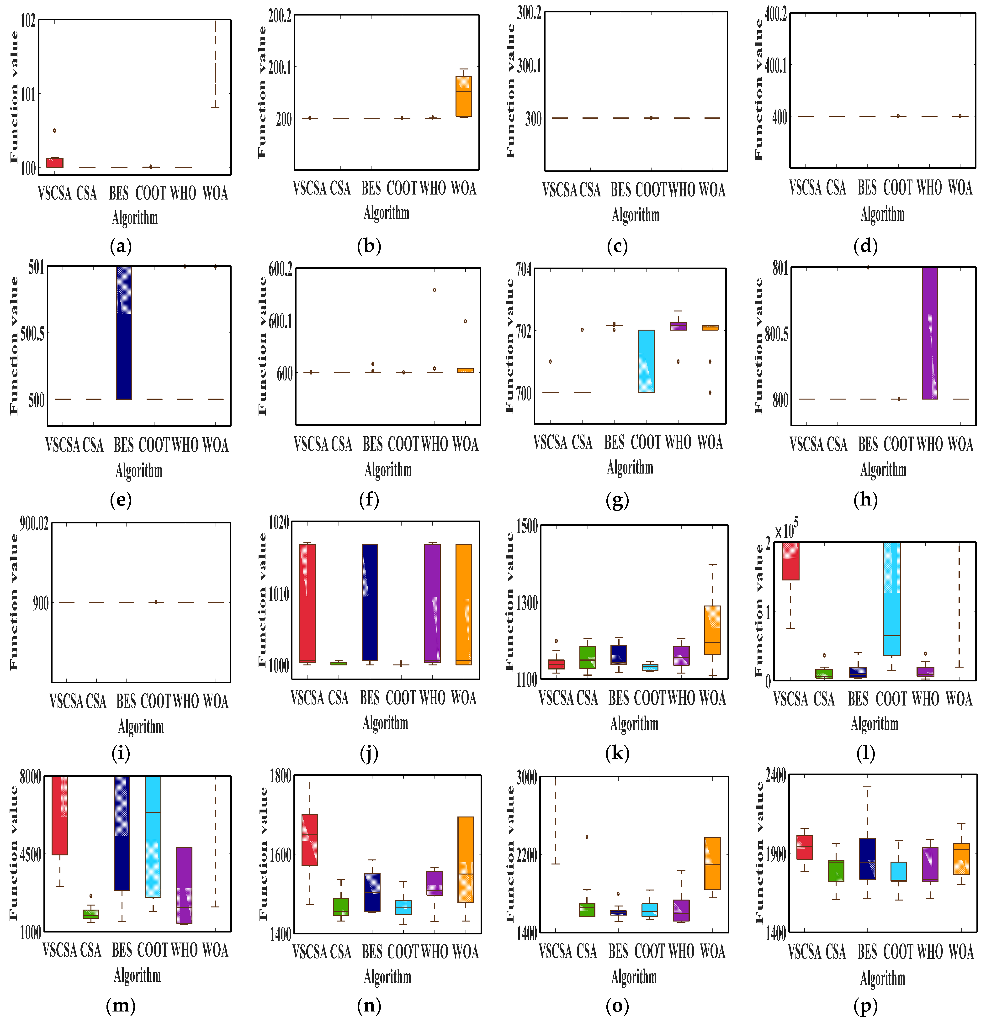
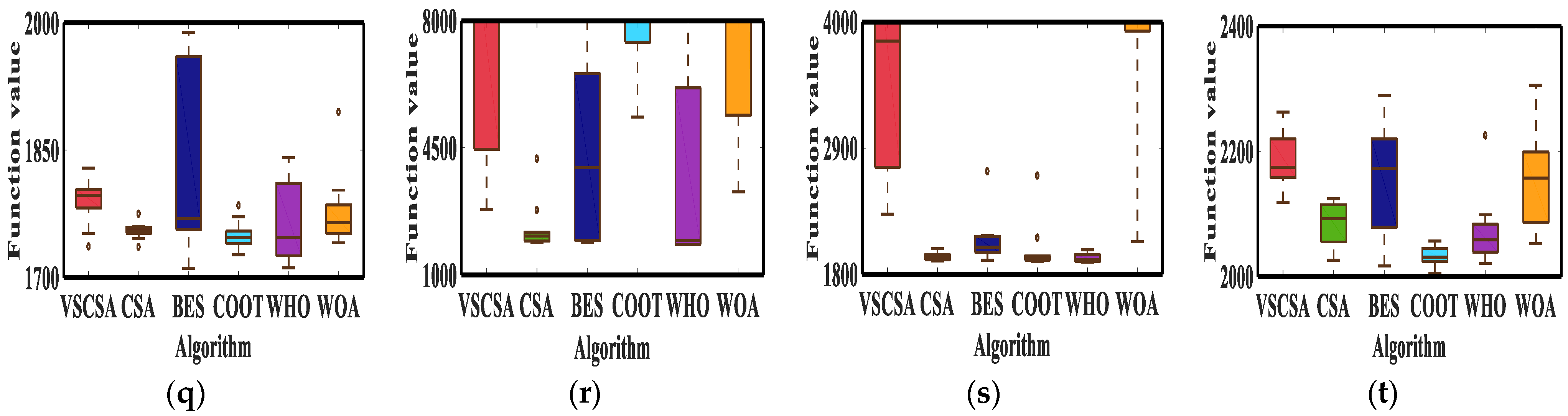
Figure 12 gives box plots for different algorithms after 10 independent runs. VSCSA has the narrowest box plot in function F2 to F9. CSA has the narrowest box plot in function F12, F13, and F18. BES has the narrowest box plot in function F15. COOT has the narrowest box plot in function F10, F11, F14, F16, F17, F19, and F20. VSCSA has the worst box plot in function F1 and F15. BES has the worst box plot in function F5, F16, F17, and F20. COOT has the worst box plot in function F7. WHO has the worst box plot in function F8. WOA has the worst box plot in function F6, F11, F12, F13, F14, F18, and F19. For F10, VSCSA, BES, WHO, and WOA have large box plots.
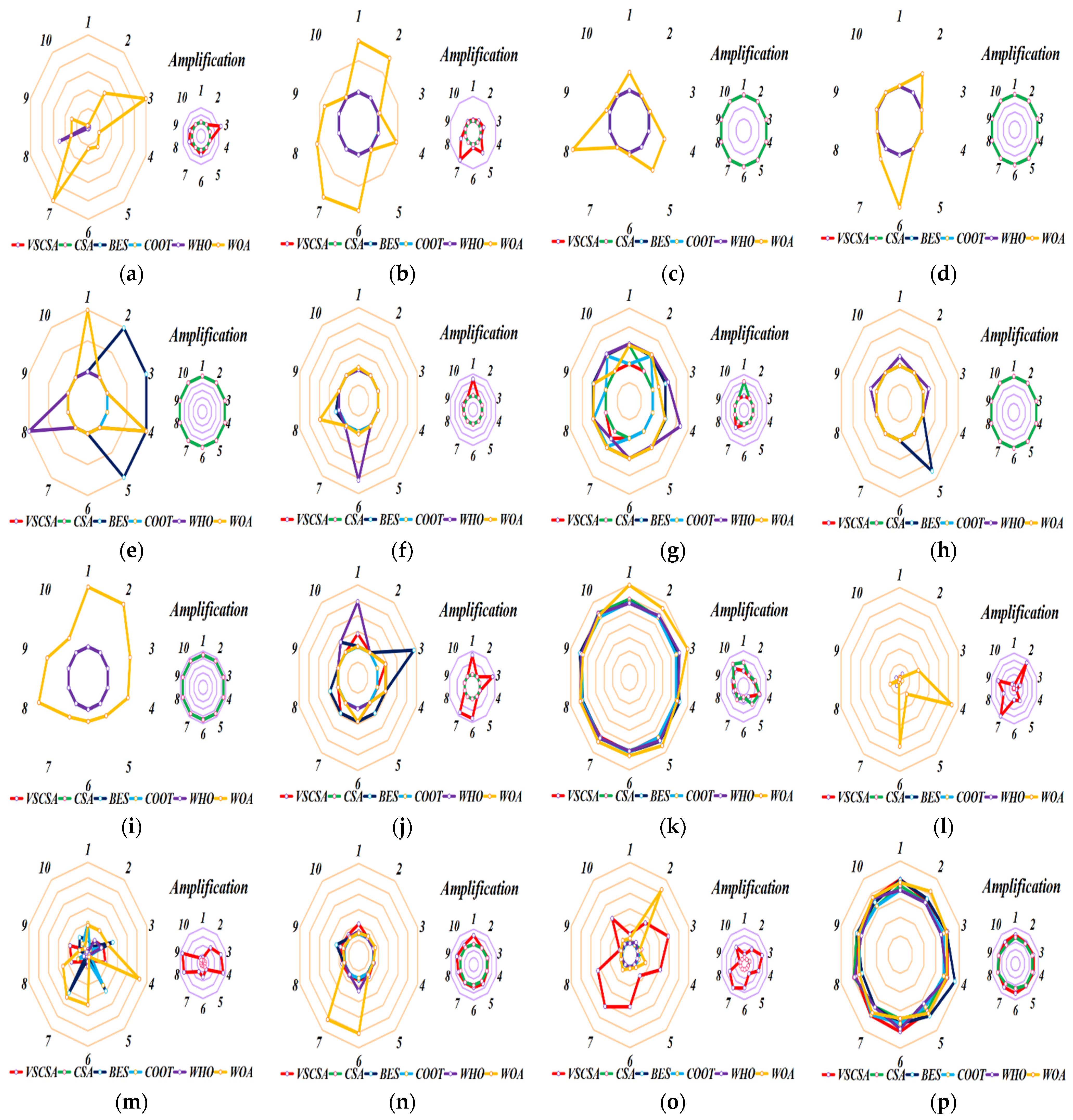
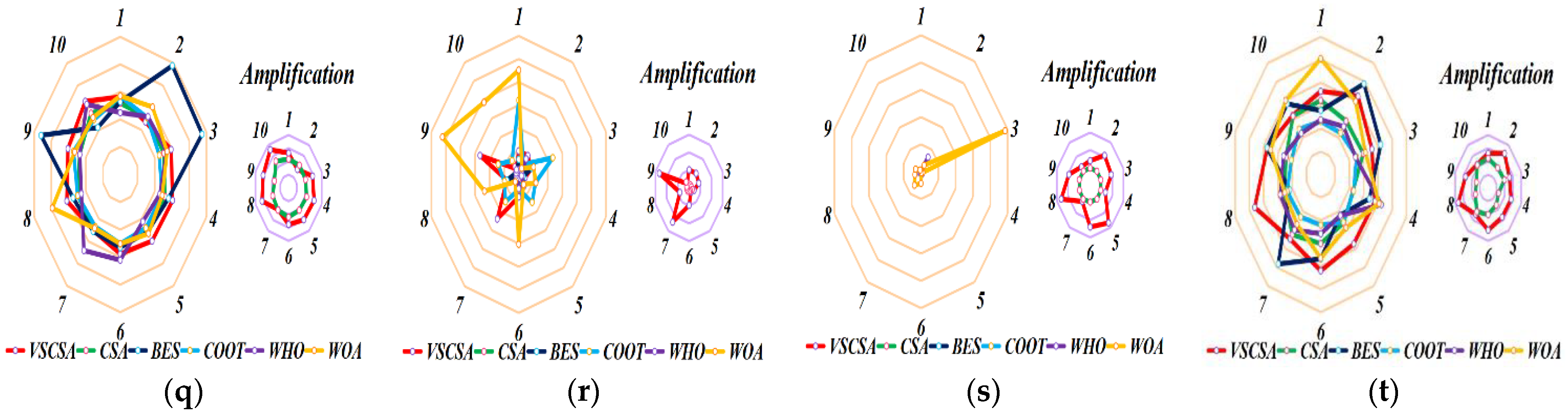
Figure 13 gives radar charts for different algorithms after 10 independent runs. For Figure 13, VSCSA subsequences have the largest radar charts for function F15. BES has the largest radar charts for function F5 and F8. WHO has the largest radar charts for function F6. WOA has the largest radar charts for function F1 to F4, F9, F12, F14, F18, and F19. For function F7, F10, F11, F13, F16, F17, and F20, many algorithms have large radar charts.
Table 7 shows the Wilcoxon rank sum test results. In Table 7, N means that the computer cannot give the p-value because of the too-large or too-small p-value. In function F7, F11, the p-value in CSA is larger than 0.05. In functions F6, F8, F10, F11, F13, F16, F17, F20, the p-value in BES is larger than 0.05. In function F1, F3, F6, F8, F9, F11, F13, F18, the p-value in COOT is larger than 0.05. In function F2, F5, F6, F8, F10, F11, F14, F17, the p-value in WHO is larger than 0.05. In function F10, F12, F10, F14, F16 to F20, the p-value in WOA is larger than 0.05. For other algorithms, the Wilcoxon rank sum test results are all less than 0.05.

Table 5.
Basic information of CEC2017 benchmark functions.
| No. | Function | D | Range | Fmin |
|---|---|---|---|---|
| F1 | Shifted and Rotated Bent Cigar Function | 2 | [−100, 100] | 100 |
| F2 | Shifted and Rotated Zakharov Function | 2 | [−100, 100] | 200 |
| F3 | Shifted and Rotated Rosenbrock’s Function | 2 | [−100, 100] | 300 |
| F4 | Shifted and Rotated Rastrigin’s Function | 2 | [−100, 100] | 400 |
| F5 | Shifted and Rotated Expanded Scaffer’s F6 Function | 2 | [−100, 100] | 500 |
| F6 | Shifted and Rotated Lunacek Bi-Rastrigin Function | 2 | [−100, 100] | 600 |
| F7 | Shifted and Rotated Non-Continuous Rastrigin’s Function | 2 | [−100, 100] | 700 |
| F8 | Shifted and Rotated Levy Function | 2 | [−100, 100] | 800 |
| F9 | Shifted and Rotated Schwefel’s Function | 2 | [−100, 100] | 900 |
| F10 | Hybrid Function 1 (N = 3) | 2 | [−100, 100] | 1000 |
| F11 | Hybrid Function 2 (N = 3) | 10 | [−100, 100] | 1100 |
| F12 | Hybrid Function 3 (N = 3) | 10 | [−100, 100] | 1200 |
| F13 | Hybrid Function 4 (N = 4) | 10 | [−100, 100] | 1300 |
| F14 | Hybrid Function 5 (N = 4) | 10 | [−100, 100] | 1400 |
| F15 | Hybrid Function 6 (N = 4) | 10 | [−100, 100] | 1500 |
| F16 | Hybrid Function 6 (N = 5) | 10 | [−100, 100] | 1600 |
| F17 | Hybrid Function 6 (N = 5) | 10 | [−100, 100] | 1700 |
| F18 | Hybrid Function 6 (N = 5) | 10 | [−100, 100] | 1800 |
| F19 | Hybrid Function 6 (N = 6) | 10 | [−100, 100] | 1900 |
| F20 | Composition Function 1 (N = 3) | 10 | [−100, 100] | 2000 |
Table 6.
Comparison of results for CEC2017 benchmark functions.
| Function | Metric | VSCSA | CSA | BES | COOT | WHO | WOA |
|---|---|---|---|---|---|---|---|
| F1 | Min | 100.0000 | 100.0000 | 100.0000 | 100.0000 | 100.0000 | 100.8089 |
| Max | 100.4967 | 100.0000 | 100.0000 | 100.0079 | 2476.9326 | 4991.5872 | |
| Var | 0.0239 | 0 | 0 | 5.8721 × 10⁻⁶ | 5.6498 × 10⁵ | 3.0578 × 10⁶ | |
| F2 | Min | 200.0000 | 200.0000 | 200.0000 | 200.0000 | 200.0000 | 200.0020 |
| Max | 200.0000 | 200.0000 | 200.0000 | 200.0000 | 200.0012 | 200.0951 | |
| Var | 3.2226 × 10⁻¹³ | 0 | 0 | 7.7463 × 10⁻¹¹ | 1.6905 × 10⁻⁷ | 1.3605 × 10⁻³ | |
| F3 | Min | 300.0000 | 300.0000 | 300.0000 | 300.0000 | 300.0000 | 300.0000 |
| Max | 300.0000 | 300.0000 | 300.0000 | 300.0000 | 300.0000 | 300.0000 | |
| Var | 0 | 0 | 0 | 3.5902 × 10⁻²⁸ | 0 | 9.2862 × 10⁻²² | |
| F4 | Min | 400.0000 | 400.0000 | 400.0000 | 400.0000 | 400.0000 | 400.0000 |
| Max | 400.0000 | 400.0000 | 400.0000 | 400.0000 | 400.0000 | 400.0000 | |
| Var | 0 | 0 | 0 | 1.3381 × 10⁻²¹ | 6.9650 × 10⁻²⁶ | 2.1903 × 10⁻¹⁴ | |
| F5 | Min | 500.0000 | 500.0000 | 500.0000 | 500.0000 | 500.0000 | 500.0000 |
| Max | 500.0000 | 500.0000 | 500.9950 | 500.0000 | 500.9950 | 500.9950 | |
| Var | 0 | 0 | 0.2640 | 0 | 0.1760 | 0.1760 | |
| F6 | Min | 600.0000 | 600.0000 | 600.0000 | 600.0000 | 600.0000 | 600.0000 |
| Max | 600.0002 | 600.0000 | 600.0164 | 600.0000 | 600.1573 | 600.0976 | |
| Var | 5.1834 × 10⁻⁹ | 0 | 2.6128 × 10⁻⁵ | 8.0042 × 10⁻¹¹ | 0.0025 | 0.0009 | |
| F7 | Min | 700.0000 | 700.0000 | 702.0163 | 700.0000 | 700.9950 | 700.0000 |
| Max | 700.9950 | 702.0163 | 702.2136 | 702.0163 | 704.7119 | 702.1708 | |
| Var | 0.0990 | 0.4066 | 0.0027 | 1.0842 | 0.8721 | 0.5292 | |
| F8 | Min | 800.0000 | 800.0000 | 800.0000 | 800.0000 | 800.0000 | 800.0000 |
| Max | 800.0000 | 800.0000 | 804.9748 | 800.0000 | 800.9950 | 800.0000 | |
| Var | 0 | 0 | 2.4639 | 5.7443 × 10⁻²⁷ | 0.2310 | 4.8755 × 10⁻²⁴ | |
| F9 | Min | 900.0000 | 900.0000 | 900.0000 | 900.0000 | 900.0000 | 900.0000 |
| Max | 900.0000 | 900.0000 | 900.0000 | 900.0000 | 900.0000 | 900.0000 | |
| Var | 0 | 0 | 0 | 5.7443 × 10⁻²⁷ | 0 | 8.2264 × 10⁻¹⁴ | |
| F10 | Min | 1000.0000 | 1000.0000 | 1000.0000 | 1000.0000 | 1000.0000 | 1000.0000 |
| Max | 1017.0694 | 1000.6243 | 1074.9496 | 1000.3122 | 1058.5045 | 1016.7572 | |
| Var | 71.9334 | 0.0444 | 465.5578 | 0.0097 | 337.6272 | 63.1675 | |
| F11 | Min | 1114.9624 | 1109.6715 | 1116.5732 | 1119.8084 | 1114.9368 | 1109.3504 |
| Max | 1198.3403 | 1204.5114 | 1207.1855 | 1144.6353 | 1204.4832 | 1396.9177 | |
| Var | 663.0311 | 1057.8398 | 958.1988 | 70.7817 | 889.1115 | 1.0239 × 10⁴ | |
| F12 | Min | 7.5856 × 10⁴ | 2604.2573 | 3128.5674 | 1.4793 × 10⁴ | 2.5114 × 10³ | 1.9748 × 10⁴ |
| Max | 9.7061 × 10⁵ | 3.6182 × 10⁴ | 4.0349 × 10⁴ | 5.7144 × 10⁵ | 3.8765 × 10⁴ | 1.0693 × 10⁷ | |
| Var | 1.0431 × 10+11 | 1.1384 × 10⁸ | 1.4756 × 10⁸ | 4.7970 × 10+10 | 1.3494 × 10⁸ | 1.48761 × 10+13 | |
| F13 | Min | 3041.5027 | 1403.7263 | 1455.2229 | 1895.3341 | 1318.7813 | 2105.0934 |
| Max | 1.8156 × 10⁴ | 2602.3091 | 3.1311 × 10⁴ | 2.5062 × 10⁴ | 1.3722 × 10⁴ | 5.2478 × 10⁴ | |
| Var | 3.8814 × 10⁷ | 1.2894 × 10⁵ | 1.3522 × 10⁸ | 6.6879 × 10⁷ | 2.0050 × 10⁷ | 2.3650 × 10⁸ | |
| F14 | Min | 1472.2338 | 1431.3035 | 1453.1541 | 1423.2821 | 1429.3626 | 1431.4869 |
| Max | 2069.1500 | 1536.7192 | 2282.9765 | 1531.6019 | 2297.9909 | 5143.6059 | |
| Var | 3.1788 × 10⁴ | 1113.3125 | 6.3312 × 10⁴ | 1214.3278 | 6.3780 × 10⁴ | 2.2832 × 10⁶ | |
| F15 | Min | 2102.0812 | 1561.6616 | 1514.5328 | 1530.4193 | 1501.4497 | 1755.3194 |
| Max | 8248.5418 | 2380.6647 | 1.7944 × 10³ | 1835.0032 | 2035.3400 | 1.0501 × 10⁴ | |
| Var | 4.5125 × 10⁶ | 6.0137 × 10⁴ | 6405.4267 | 9095.8887 | 2.7671 × 10⁴ | 7.1257 × 10⁶ | |
| F16 | Min | 1785.9923 | 1605.1444 | 1614.9232 | 1604.0291 | 1614.1054 | 1703.0662 |
| Max | 2058.8581 | 1962.8200 | 2319.6410 | 1980.6734 | 1989.2964 | 2086.8136 | |
| Var | 9501.8979 | 1.0527 × 10⁴ | 3.8956 × 10⁴ | 1.0911 × 10⁴ | 1.9357 × 10⁴ | 1.4474 × 10⁴ | |
| F17 | Min | 1736.2506 | 1735.7399 | 1711.0671 | 1726.6221 | 1711.3399 | 1741.0307 |
| Max | 1828.8309 | 1774.8088 | 1988.8544 | 1784.6624 | 1841.2146 | 1894.6790 | |
| Var | 756.9156 | 102.0301 | 1.1332 × 10⁴ | 297.7841 | 2068.8956 | 2046.5244 | |
| F18 | Min | 2795.7978 | 1899.0415 | 1900.8064 | 5348.1482 | 1837.5630 | 3284.2186 |
| Max | 2.6628 × 10⁴ | 4194.3397 | 9071.9493 | 3.2147 × 10⁴ | 8313.3384 | 5.2491 × 10⁴ | |
| Var | 6.6663 × 10⁷ | 4.9868 × 10⁵ | 7.3939 × 10⁶ | 6.8506 × 10⁷ | 6.0211 × 10⁶ | 3.3418 × 10⁸ | |
| F19 | Min | 2323.2878 | 1914.0998 | 1919.9589 | 1906.5796 | 1905.3476 | 2080.4660 |
| Max | 5351.9820 | 2022.0524 | 2.6936 × 10³ | 2656.9216 | 3.2933 × 10⁴ | 2.4271 × 10⁵ | |
| Var | 1.2781 × 10⁶ | 1145.4605 | 4.8170 × 10⁴ | 5.2873 × 10⁴ | 9.6078 × 10⁷ | 5.3813 × 10⁹ | |
| F20 | Min | 2118.6468 | 2025.8065 | 2016.9142 | 2004.9954 | 2020.8626 | 2052.4900 |
| Max | 2262.7814 | 2123.8647 | 2289.2135 | 2056.6773 | 2224.7862 | 2305.7172 | |
| Var | 1758.7689 | 1230.6049 | 9242.5172 | 231.5231 | 3534.4072 | 5965.3790 |
Table 7.
Comparison of the Wilcoxon rank sum test results in CEC2017 functions.
| Function | CSA | BES | COOT | WHO | WOA |
|---|---|---|---|---|---|
| F1 | 0.00075 | 0.00075 | 0.51989 | 0.02384 | 0.00018 |
| F2 | 0.00006 | 0.00006 | 0.03764 | 0.47100 | 0.00018 |
| F3 | N | N | 0.36812 | N | 0.00006 |
| F4 | N | N | 0.03498 | 0.01493 | 0.00006 |
| F5 | N | 0.03359 | N | 0.16749 | 0.00023 |
| F6 | 0.01493 | 0.57148 | 0.10957 | 0.39943 | 0.00069 |
| F7 | 1.00000 | 0.00007 | 0.04981 | 0.00010 | 0.00012 |
| F8 | N | 0.16808 | 0.36812 | 0.07672 | 0.00023 |
| F9 | N | N | 0.36812 | N | 0.00006 |
| F10 | 0.00978 | 0.35909 | 0.00445 | 1.00000 | 0.96975 |
| F11 | 0.52052 | 0.42736 | 0.34470 | 0.27304 | 0.01726 |
| F12 | 0.00018 | 0.00018 | 0.04515 | 0.00018 | 0.42736 |
| F13 | 0.00018 | 0.96985 | 0.42736 | 0.01402 | 0.03764 |
| F14 | 0.00101 | 0.03121 | 0.00077 | 0.06402 | 0.30749 |
| F15 | 0.00025 | 0.00018 | 0.00018 | 0.00018 | 0.00911 |
| F16 | 0.00911 | 0.27304 | 0.00361 | 0.01726 | 0.47268 |
| F17 | 0.01402 | 0.57075 | 0.00459 | 0.18588 | 0.14047 |
| F18 | 0.00033 | 0.02113 | 0.27304 | 0.00283 | 0.12122 |
| F19 | 0.00018 | 0.00033 | 0.00033 | 0.00283 | 0.05390 |
| F20 | 0.00033 | 0.73373 | 0.00018 | 0.00220 | 0.34470 |
6. Engineering Applications
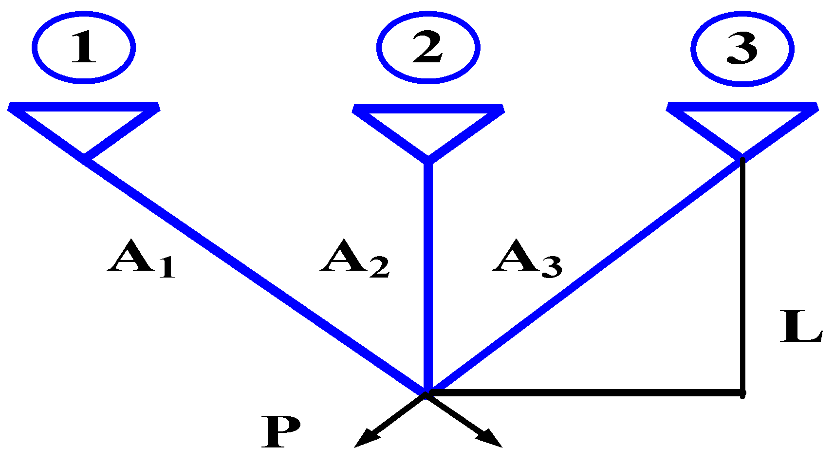
6.1. Three Bar Truss Design Problem
The three bar truss design problem is a civil engineering problem, and the weight of the bar structure is the key problem in the Gear Train Problem which owns a problematic and constrained space. The constraints of this problem are based on the stress constraints of each bar. Figure 14 is the structural diagram of the three bar truss design problem. A1 A2 A3 respectively represents the length of the bar, P means the force value, L means the space length.
This problem can be described mathematically as follows:
In this paper, basic CSA were selected for the CSA literature. Comparison algorithms and parameters selected the algorithm literature [50], with each method tested 30 times with 1000 iterations and a maximum of 60,000 number function evaluations (NFEs). The results of best, mean, minimum values, maximum values, and the standard deviation value are given in Table 8.
The VSCSA Min value is the same as the CSA Min value and the WHO Min value. The VSCSA Max value is larger than the CSA Max value. WHO and CSA obtain the less Max value and the Avg value. WHO obtains the less Std value. AEFA obtains the worst Min value, the Max value, the Std value, and the Avg value.
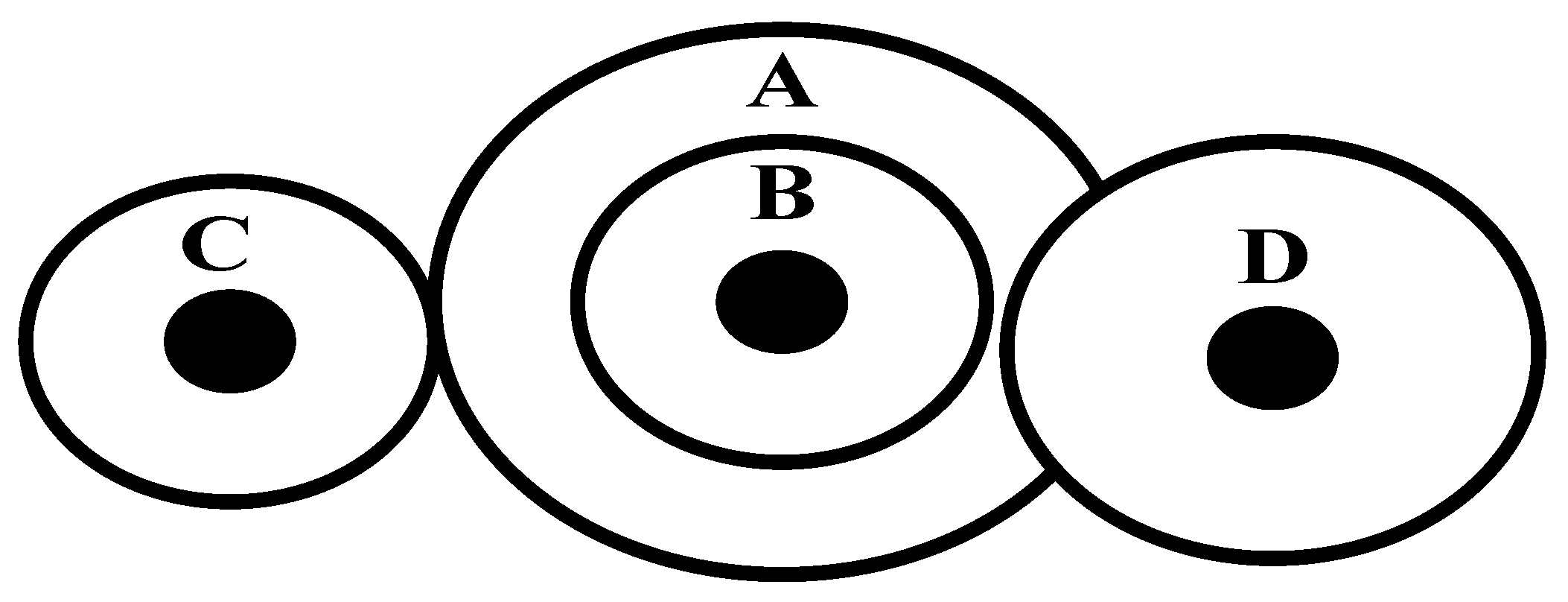
6.2. The Gear Train Problem
The cost of the gear ratio of the gear train is the key problem in the Gear Train Problem which owns only four parameters in boundary constraints. Four parameters are discrete because each gear should have an integral number of teeth in this problem. Discrete variables add different complexities for this problem. Figure 15 is the structural diagram of the Gear Train Problem. Four parameters are the numbers of teeth on the gears: nA, nB, nC, and nD. A, B, C, and D mean centre points.
This problem can be described mathematically as follows:
In this paper, basic CSA was selected for the CSA literature. Comparison algorithms and parameters selected the algorithm literature, the number of population sizes is set to 50, and the maximum number of iterations is set to 1000. All algorithms are executed for 30 independent runs. The results of the best, mean, minimum values, maximum values, and the standard deviation value are given in Table 9. Comparison algorithms include CS [46], FPA [50], FSA [51], SA [52], and SCA [14]. The VSCSA Min value is the same as the CSA Min value. SCA obtains the worst Min value. SCA obtains the worst Max value, Std value, and Avg value. The VSCSA Min value, Max value, Std value, and Avg value are larger than those of CSA. There is no specific algorithm that can perfectly solve all engineering problems. Different algorithms can be selected for different engineering problems.
7. Conclusions
In this paper, VSCSA is introduced to solve function problems. The proposed algorithm uses the cosine function to enhance the CSA searching ability. VSCSA has strong problem applicability and can effectively find the global optimum in a short iteration period, greatly improving the solution accuracy. In conclusion, the proposed algorithm VSCSA has significant advantages over CSA in CEC-2017 fitness values, iteration curves, box plots, and search paths. In addition, the Wilcoxon test results statistically indicate differences between VSCSA and other comparative algorithms. Engineering applications show that the proposed algorithm has strong competitiveness. The above data and conclusions indicate that the improvement strategy proposed in this paper has achieved good results, greatly improving the performances of the original CSA. Many algorithms have been applied to specific fields such as medicine, aerospace, and industry and have achieved good results. Therefore, combining VSCSA with practical problems in specific fields is a direction for future research.
Author Contributions
Conceptualization, Y.F.; methodology, Y.F.; formal analysis, H.Y.; investigation, Z.X.; resources, Y.W. and Y.F.; writing—original draft preparation, Y.F.; writing—review and editing, H.Y. and Z.X.; visualization, D.L.; supervision, Y.W.; project administration, Y.W.; funding acquisition, Y.W and Y.F. All authors have read and agreed to the published version of the manuscript.
Funding
This research was funded by the National Natural Science Foundation of China, grant number 52175502, as well as the Natural Science Foundation of Heilongjiang Province, grant number LH2023E082, in addition to the basic research business fee projects of provincial undergraduate universities in Heilongjiang Province, grant number 2022-KYYWF-0144.
Institutional Review Board Statement
Not applicable.
Data Availability Statement
The data used to support the findings of this study are included in this article.
Conflicts of Interest
The authors declare no conflict of interest.
References
- Ray, T.; Liew, K.M. Society and civilization: An optimization algorithm based on the simulation of social behavior. IEEE Trans. Evol. Comput. 2003, 7, 386–396. [Google Scholar] [CrossRef]
- Iba, K. Reactive power optimization by genetic algorithm. IEEE Trans. Power Syst. 1994, 9, 685–692. [Google Scholar] [CrossRef]
- Mafarja, M.; Aljarah, I.; Heidari, A.A.; Hammouri, A.I.; Faris, H.; Al-Zoubi, A.M.; Mirjalili, S. Evolutionary Population Dynamics and Grasshopper Optimization approaches for feature selection problems. Knowl. Based Syst. 2018, 145, 25–45. [Google Scholar] [CrossRef]
- Mirjalili, S.; Gandomi, A.H.; Mirjalili, S.Z.; Saremi, S.; Faris, H.; Mirjalili, S.M. Salp Swarm Algorithm: A bio-inspired optimizer for engineering design problems. Adv. Eng. Softw. 2017, 114, 163–191. [Google Scholar] [CrossRef]
- Wolpert, D.H.; Macready, W.G. No free lunch theorems for optimization. IEEE Trans. Evol. Comput. 1997, 1, 67–82. [Google Scholar] [CrossRef]
- Borchers, A.; Pieler, T. Programming pluripotent precursor cells derived from Xenopus embryos to generate specific tissues and organs. Genes 2010, 1, 413–426. [Google Scholar] [CrossRef]
- Storn, R.; Price, K. Differential Evolution-A Simple and Efficient Heuristic for global Optimization over Continuous Spaces. J. Glob. Optim. 1997, 11, 341–359. [Google Scholar] [CrossRef]
- Abdollahzadeh, B.; Gharehchopogh, F.S.; Mirjalili, S. African vultures optimization algorithm: A new nature-inspired metaheuristic algorithm for global optimization problems. Comput. Ind. Eng. 2021, 158, 107408. [Google Scholar] [CrossRef]
- Zhong, C.; Li, G.; Meng, Z. Beluga whale optimization: A novel nature-inspired metaheuristic algorithm. Knowl. Based Syst. 2022, 251, 109215. [Google Scholar] [CrossRef]
- Mirjalili, S.; Lewis, A. The Whale Optimization Algorithm. Adv. Eng. Softw. 2016, 95, 51–67. [Google Scholar] [CrossRef]
- Karami, H.; Anaraki, M.V.; Farzin, S.; Mirjalili, S. Flow Direction Algorithm (FDA): A Novel Optimization Approach for Solving Optimization Problems. Comput. Ind. Eng. 2021, 156, 107224. [Google Scholar] [CrossRef]
- Mirjalili, S.; Mirjalili, S.M.; Lewis, A. Grey Wolf Optimizer. Adv. Eng. Softw. 2014, 69, 46–61. [Google Scholar] [CrossRef]
- Heidari, A.A.; Mirjalili, S.; Faris, H.; Aljarah, I.; Mafarja, M.; Chen, H. Harris hawks optimization: Algorithm and applications. Future Gener. Comput. Syst. 2019, 97, 849–872. [Google Scholar] [CrossRef]
- Mirjalili, S. SCA: A Sine Cosine Algorithm for Solving Optimization Problems. Knowl. Based Syst. 2016, 96, 120–133. [Google Scholar] [CrossRef]
- Dhiman, G.; Kumar, V. Spotted hyena optimizer: A novel bio-inspired based metaheuristic technique for engineering applications. Adv. Eng. Softw. 2017, 114, 48–70. [Google Scholar] [CrossRef]
- Li, S.; Chen, H.; Wang, M.; Heidari, A.A.; Mirjalili, S. Slime mould algorithm: A new method for stochastic optimization. Future Gener. Comput. Syst. 2020, 111, 300–323. [Google Scholar] [CrossRef]
- Cheng, M.-Y.; Prayogo, D. Symbiotic Organisms Search: A new metaheuristic optimization algorithm. Comput. Struct. 2014, 139, 98–112. [Google Scholar] [CrossRef]
- Naruei, I.; Keynia, F. Wild horse optimizer: A new meta-heuristic algorithm for solving engineering optimization problems. Eng. Comput. 2021, 38, 3025–3056. [Google Scholar] [CrossRef]
- Rezaei, F.; Safavi, H.R.; Abd Elaziz, M.; Mirjalili, S. GMO: Geometric mean optimizer for solving engineering prob lems. Soft Comput. 2023, 27, 10571–10606. [Google Scholar] [CrossRef]
- Chopra, N.; Ansari, M.M. Golden jackal optimization: A novel nature-inspired optimizer for engineering applications. Expert Syst. Appl. 2022, 198, 116924. [Google Scholar] [CrossRef]
- Dehghani, M.; Trojovska, E.; Trojovsky, P.; Montazeri, Z. Coati Optimization Algorithm: A new bio-inspired metaheuristic algorithm for solving optimization problems. Knowl.-Based Syst. 2023, 259, 110011. [Google Scholar] [CrossRef]
- Zhao, S.; Zhang, T.; Ma, S.; Chen, M. Dandelion Optimizer: A nature-inspired metaheuristic algorithm for engineering applications. Eng. Appl. Artif. Intell. Int. J. Intell. Real-Time Autom. 2022, 114, 105075. [Google Scholar] [CrossRef]
- Jia, H.; Peng, X.; Lang, C. Remora Optimization Algorithm. Expert Syst. Appl. 2021, 185, 115665. [Google Scholar] [CrossRef]
- Guan, Z.; Ren, C.; Niu, J.; Wang, P.; Shang, Y. Great Wall Construction Algorithm: A novel meta-heuristic algorithm for engineer problems. Expert Syst. Appl. 2023, 233, 120905. [Google Scholar] [CrossRef]
- Zhang, Y.; Jin, Z.; Mirjalili, S. Generalized normal distribution optimization and its applications in parameter extraction of photovoltaic models. Energy Convers. Manag. 2020, 224, 113301. [Google Scholar] [CrossRef]
- Trojovsky, P.; Dehghani, M. Pelican Optimization Algorithm: A Novel Nature-Inspired Algorithm for Engineering Applications. Sensors 2022, 22, 855. [Google Scholar] [CrossRef] [PubMed]
- Moosavi, S.H.S.; Bardsiri, V.K. Satin bowerbird optimizer: A new optimization algorithm to optimize ANFIS for software development effort estimation. Eng. Appl. Artif. Intell. 2017, 60, 1–15. [Google Scholar] [CrossRef]
- Rao, R.V.; Savsani, V.J.; Vakharia, D.P. Teaching–Learning-Based Optimization: An optimization method for continuous non-linear large scale problems. Inf. Sci. 2012, 183, 1–15. [Google Scholar] [CrossRef]
- Seyyedabbasi, A.; Kiani, F. Sand Cat swarm optimization: A nature-inspired algorithm to solve global optimization problems. Eng. Comput. 2022, 39, 2627–2651. [Google Scholar] [CrossRef]
- Jiang, X.; Lin, Z.; He, T.; Ma, X.; Ma, S.; Li, S. Optimal Path Finding With Beetle Antennae Search Algorithm by Using Ant Colony Optimization Initialization and Different Searching Strategies. IEEE Access 2020, 8, 15459–15471. [Google Scholar] [CrossRef]
- Pan, H.; Gong, J. Application of Particle Swarm Optimization (PSO) Algorithm in Determining Thermodynamics of Solid Combustibles. Energies 2023, 16, 5302. [Google Scholar] [CrossRef]
- Zandavi, S.M.; Chung, V.Y.Y.; Anaissi, A. Stochastic Dual Simplex Algorithm: A Novel Heuristic Optimization Algorithm. IEEE Trans. Cybern. 2021, 51, 2725–2734. [Google Scholar] [CrossRef] [PubMed]
- Liang, X.; Cai, Z.; Wang, M.; Zhao, X.; Chen, H.; Li, C. Chaotic oppositional sine–cosine method for solving global optimization problems. Eng. Comput. 2020, 38, 1223–1239. [Google Scholar] [CrossRef]
- Pazhaniraja, N.; Basheer, S.; Thirugnanasambandam, K.; Ramalingam, R.; Rashid, M.; Kalaivani, J. Multi-objective Boolean grey wolf optimization based decomposition algorithm for high-frequency and high-utility itemset mining. AIMS Math. 2023, 8, 18111–18140. [Google Scholar] [CrossRef]
- Huang, Z.; Li, F.; Zhu, L.; Ye, G.; Zhao, T. Phase Mask Design Based on an Improved Particle Swarm Optimization Algorithm for Depth of Field Extension. Appl. Sci. 2023, 13, 7899. [Google Scholar] [CrossRef]
- Akın, P. A new hybrid approach based on genetic algorithm and support vector machine methods for hyperparameter optimization in synthetic minority over-sampling technique (SMOTE). AIMS Math. 2023, 8, 9400–9415. [Google Scholar] [CrossRef]
- Askarzadeh, A. A novel metaheuristic method for solving constrained engineering optimization problems: Crow search algorithm. Comput. Struct. 2016, 169, 1–12. [Google Scholar] [CrossRef]
- Shekhawat, S.; Saxena, A. Development and applications of an intelligent crow search algorithm based on opposition based learning. ISA Trans. 2020, 99, 210–230. [Google Scholar] [CrossRef] [PubMed]
- Chen, Y.; Ye, Z.; Gao, B.; Wu, Y.; Yan, X.; Liao, X. A Robust Adaptive Hierarchical Learning Crow Search Algorithm for Feature Selection. Electronics 2023, 12, 3123. [Google Scholar] [CrossRef]
- Díaz, P.; Pérez-Cisneros, M.; Cuevas, E.; Avalos, O.; Gálvez, J.; Hinojosa, S.; Zaldivar, D. An Improved Crow Search Algorithm Applied to Energy Problems. Energies 2018, 11, 571. [Google Scholar] [CrossRef]
- Bhullar, A.K.; Kaur, R.; Sondhi, S. Enhanced crow search algorithm for AVR optimization. Soft Comput. 2020, 24, 11957–11987. [Google Scholar] [CrossRef]
- Gadekallu, T.R.; Alazab, M.; Kaluri, R.; Maddikunta, P.K.R.; Bhattacharya, S.; Lakshmanna, K.; M, P. Hand gesture classification using a novel CNN-crow search algorithm. Complex Intell. Syst. 2021, 7, 1855–1868. [Google Scholar] [CrossRef]
- Braik, M.; Al-Zoubi, H.; Ryalat, M.; Sheta, A.; Alzubi, O. Memory based hybrid crow search algorithm for solving numerical and constrained global optimization problems. Artif. Intell. Rev. 2022, 56, 27–99. [Google Scholar] [CrossRef]
- Samieiyan, B.; MohammadiNasab, P.; Mollaei, M.A.; Hajizadeh, F.; Kangavari, M. Solving dimension reduction problems for classification using Promoted Crow Search Algorithm (PCSA). Computing 2022, 104, 1255–1284. [Google Scholar] [CrossRef]
- Guo, Q.; Chen, H.; Luo, J.; Wang, X.; Wang, L.; Lv, X.; Wang, L. Parameter inversion of probability integral method based on improved crow search algorithm. Arab. J. Geosci. 2022, 15, 180. [Google Scholar] [CrossRef]
- Gandomi, A.H.; Yang, X.-S.; Alavi, A.H. Cuckoo search algorithm: A metaheuristic approach to solve structural optimization problems. Eng. Comput. 2013, 29, 17–35. [Google Scholar] [CrossRef]
- Mirjalili, S. Moth-flame optimization algorithm: A novel nature-inspired heuristic paradigm. Knowl. Based Syst. 2015, 89, 228–249. [Google Scholar] [CrossRef]
- Alsattar, H.A.; Zaidan, A.A.; Zaidan, B.B. Novel meta-heuristic bald eagle search optimisation algorithm. Artif. Intell. Rev. 2020, 53, 2237–2264. [Google Scholar] [CrossRef]
- Naruei, I.; Keynia, F. A New Optimization Method Based on Coot Bird Natural Life Model. Expert Syst. Appl. 2021, 183, 115352. [Google Scholar] [CrossRef]
- Yang, X.-S.; Karamanoglu, M.; He, X. Flower pollination algorithm: A novel approach for multiobjective optimiza tion. Eng. Optim. 2014, 46, 1222–1237. [Google Scholar] [CrossRef]
- Elsisi, M. Future search algorithm for optimization. Evol. Intell. 2018, 12, 21–31. [Google Scholar] [CrossRef]
- Osman, I.H. Metastrategy simulated annealing and tabu search algorithms for the vehicle routing problem. Ann. Oper. Res. 1993, 41, 421–451. [Google Scholar] [CrossRef]
Figure 1.
The VSCSA Flowchart.

Figure 2.
Iteration curves of two−dimension functions. (a) f1; (b) f2; (c) f3; (d) f4; (e) f5; (f) f6; (g) f7; (h) f8; (i) f9; (j) f10; (k) f11(D=2); (l) f12(D=2); (m) f13(D=2); (n) f14(D=2).
Figure 2.
Iteration curves of two−dimension functions. (a) f1; (b) f2; (c) f3; (d) f4; (e) f5; (f) f6; (g) f7; (h) f8; (i) f9; (j) f10; (k) f11(D=2); (l) f12(D=2); (m) f13(D=2); (n) f14(D=2).

Figure 3.
Iteration curves of high−dimension functions. (a) f11(D=30); (b) f12(D=30); (c) f13(D=30); (d) f14(D=30); (e) f11(D=60); (f) f12(D=60); (g) f13(D=60); (h) f14(D=60); (i) f11(D=200); (j) f12(D=200); (k) f13(D=200); (l) f14(D=200).
Figure 3.
Iteration curves of high−dimension functions. (a) f11(D=30); (b) f12(D=30); (c) f13(D=30); (d) f14(D=30); (e) f11(D=60); (f) f12(D=60); (g) f13(D=60); (h) f14(D=60); (i) f11(D=200); (j) f12(D=200); (k) f13(D=200); (l) f14(D=200).

Figure 4.
Box plot charts of two−dimension functions. (a) f1; (b) f2; (c) f3; (d) f4; (e) f5; (f) f6; (g) f7; (h) f8; (i) f9; (j) f10; (k) f11(D=2); (l) f12(D=2); (m) f13(D=2); (n) f14(D=2).
Figure 4.
Box plot charts of two−dimension functions. (a) f1; (b) f2; (c) f3; (d) f4; (e) f5; (f) f6; (g) f7; (h) f8; (i) f9; (j) f10; (k) f11(D=2); (l) f12(D=2); (m) f13(D=2); (n) f14(D=2).

Figure 5.
Box plot charts of high−dimension functions. (a) f11(D=30); (b) f12(D=30); (c) f13(D=30); (d) f14(D=30); (e) f11(D=60); (f) f12(D=60); (g) f13(D=60); (h) f14(D=60); (i) f11(D=200); (j) f12(D=200); (k) f13(D=200); (l) f14(D=200).
Figure 5.
Box plot charts of high−dimension functions. (a) f11(D=30); (b) f12(D=30); (c) f13(D=30); (d) f14(D=30); (e) f11(D=60); (f) f12(D=60); (g) f13(D=60); (h) f14(D=60); (i) f11(D=200); (j) f12(D=200); (k) f13(D=200); (l) f14(D=200).

Figure 6.
Sub-sequence runs radar charts of two−dimension functions. (a) f1; (b) f2; (c) f3; (d) f4; (e) f5; (f) f6; (g) f7; (h) f8; (i) f9; (j) f10; (k) f11(D=2); (l) f12(D=2); (m) f13(D=2); (n) f14(D=2).
Figure 6.
Sub-sequence runs radar charts of two−dimension functions. (a) f1; (b) f2; (c) f3; (d) f4; (e) f5; (f) f6; (g) f7; (h) f8; (i) f9; (j) f10; (k) f11(D=2); (l) f12(D=2); (m) f13(D=2); (n) f14(D=2).

Figure 7.
Sub-sequence runs radar charts of high−dimension functions. (a) f11(D=30); (b) f12(D=30); (c) f13(D=30); (d) f14(D=30); (e) f11(D=60); (f) f12(D=60); (g) f13(D=60); (h) f14(D=60); (i) f11(D=200); (j) f12(D=200); (k) f13(D=200); (l) f14(D=200).
Figure 7.
Sub-sequence runs radar charts of high−dimension functions. (a) f11(D=30); (b) f12(D=30); (c) f13(D=30); (d) f14(D=30); (e) f11(D=60); (f) f12(D=60); (g) f13(D=60); (h) f14(D=60); (i) f11(D=200); (j) f12(D=200); (k) f13(D=200); (l) f14(D=200).

Figure 8.
Three−dimension images of two-dimension functions. (a) f1; (b) f2; (c) f3; (d) f4; (e) f5; (f) f6; (g) f7; (h) f8; (i) f9; (j) f10; (k) f11(D=2); (l) f12(D=2); (m) f13(D=2); (n) f14(D=2).
Figure 8.
Three−dimension images of two-dimension functions. (a) f1; (b) f2; (c) f3; (d) f4; (e) f5; (f) f6; (g) f7; (h) f8; (i) f9; (j) f10; (k) f11(D=2); (l) f12(D=2); (m) f13(D=2); (n) f14(D=2).

Figure 9.
Search paths. (a) f1; (b) f2; (c) f3; (d) f4; (e) f5; (f) f6; (g) f7; (h) f8; (i) f9; (j) f10; (k) f11(D=2); (l) f12(D=2); (m) f13(D=2); (n) f14(D=2).
Figure 9.
Search paths. (a) f1; (b) f2; (c) f3; (d) f4; (e) f5; (f) f6; (g) f7; (h) f8; (i) f9; (j) f10; (k) f11(D=2); (l) f12(D=2); (m) f13(D=2); (n) f14(D=2).

Figure 10.
Algorithm ranking figures. (a) Two-dimension functions. (b) High-dimension functions.

Figure 11.
Iteration curves of CEC2017 functions. (a) F1; (b) F2; (c) F3; (d) F4; (e) F5; (f) F6; (g) F7; (h) F8; (i) F9; (j) F10; (k) F11; (l) F12; (m) F13; (n) F14; (o) F15; (p) F16; (q) F17; (r) F18; (s) F19; (t) F20.
Figure 11.
Iteration curves of CEC2017 functions. (a) F1; (b) F2; (c) F3; (d) F4; (e) F5; (f) F6; (g) F7; (h) F8; (i) F9; (j) F10; (k) F11; (l) F12; (m) F13; (n) F14; (o) F15; (p) F16; (q) F17; (r) F18; (s) F19; (t) F20.


Figure 12.
Box plot charts of CEC2017 functions. (a) F1; (b) F2; (c) F3; (d) F4; (e) F5; (f) F6; (g) F7; (h) F8; (i) F9; (j) F10; (k) F11; (l) F12; (m) F13; (n) F14; (o) F15; (p) F16; (q) F17; (r) F18; (s) F19; (t) F20.
Figure 12.
Box plot charts of CEC2017 functions. (a) F1; (b) F2; (c) F3; (d) F4; (e) F5; (f) F6; (g) F7; (h) F8; (i) F9; (j) F10; (k) F11; (l) F12; (m) F13; (n) F14; (o) F15; (p) F16; (q) F17; (r) F18; (s) F19; (t) F20.


Figure 13.
Sub-sequence runs radar charts of CEC2017 functions. (a) F1; (b) F2; (c) F3; (d) F4; (e) F5; (f) F6; (g) F7; (h) F8; (i) F9; (j) F10; (k) F11; (l) F12; (m) F13; (n) F14; (o) F15; (p) F16; (q) F17; (r) F18; (s) F19; (t) F20.
Figure 13.
Sub-sequence runs radar charts of CEC2017 functions. (a) F1; (b) F2; (c) F3; (d) F4; (e) F5; (f) F6; (g) F7; (h) F8; (i) F9; (j) F10; (k) F11; (l) F12; (m) F13; (n) F14; (o) F15; (p) F16; (q) F17; (r) F18; (s) F19; (t) F20.


Figure 14.
Three bar truss design problem.

Figure 15.
Gear train problem.

Table 1.
Basic information of benchmark functions.
| Name | Function | D | Range | fmin |
|---|---|---|---|---|
| Beale | f1(x) = (1.5 − + )2 + (2.25 − + )2 + (2.625 − + )2 | 2 | [−50, 50] | 0 |
| Bohachevsky01 | f2(x) = + 2 − 0.3cos(3π) − 0.4cos(4π) + 0.7 | 2 | [−50, 50] | 0 |
| Bohachevsky02 | f3(x) = + 2 − 0.3cos(3π) cos(4π) + 0.3 | 2 | [−50, 50] | 0 |
| Bohachevsky03 | f4(x) = + 2 − 0.3cos(3πx1 + 4π) + 0.3 | 2 | [−50, 50] | 0 |
| Booth | f5(x) = ( + 2x2 − 7)2 + (2x1 + x2 − 5)2 | 2 | [−50, 50] | 0 |
| Brent | f6(x) = ( + 10)2 + ( + 10)2 + e−− | 2 | [−50, 50] | 0 |
| Cube | f7(x) = 100(x2 − )2 + (1 − )2 | 2 | [−50, 50] | 0 |
| Leon | f8 (x) = 100(x2 − )2 + (1 − )2 | 2 | [−50, 50] | 0 |
| Levy13 | f9(x) = sin2(3πx1) + (x1 − 1)2[1 + sin2(3πx2)] + (x2 − 1)2[1 + sin2(2πx2)] | 2 | [−50, 50] | 0 |
| Matyas | f10(x) = 0.26( + ) − 0.48 | 2 | [−50, 50] | 0 |
| Ackley 01 | 2/30/60/200 | [−20, 20] | 0 | |
| Griewank | 2/30/60/200 | [−20, 20] | 0 | |
| Rastrigin | 2/30/60/200 | [−20, 20] | 0 | |
| Sphere | 2/30/60/200 | [−20, 20] | 0 |
Table 2.
Comparison of results for two-dimension functions.
| Function | Metric | VSCSA | CSA | CS | MFO | SCA |
|---|---|---|---|---|---|---|
| f1 | Min | 1.2634 × 10⁻³¹ | 1.1569 × 10⁻¹⁶ | 0.0436 | 8.2737 × 10⁻²² | 0.0001 |
| Max | 6.4206 × 10⁻¹⁶ | 8.2586 × 10⁻¹⁵ | 1.8208 | 0.0358 | 0.0035 | |
| Ave | 7.9525 × 10⁻¹⁷ | 2.6914 × 10⁻¹⁵ | 0.4393 | 0.0036 | 0.0009 | |
| Var | 4.1382 × 10⁻³² | 7.2893 × 10⁻³⁰ | 0.2594 | 0.0001 | 1.2328 × 10⁻⁶ | |
| f2 | Min | 0 | 2.2204 × 10⁻¹⁶ | 0.5852 | 0 | 0 |
| Max | 0 | 2.6645 × 10⁻¹⁴ | 3.4157 | 0 | 0 | |
| Ave | 0 | 7.3053 × 10⁻¹⁵ | 1.7169 | 0 | 0 | |
| Var | 0 | 7.5842 × 10⁻²⁹ | 1.2711 | 0 | 0 | |
| f3 | Min | 0 | 1.6653 × 10⁻¹⁶ | 0.0910 | 0 | 0 |
| Max | 0 | 3.9351 × 10⁻¹² | 2.0767 | 0 | 0 | |
| Ave | 0 | 5.8736 × 10⁻¹³ | 1.1458 | 0 | 0 | |
| Var | 0 | 1.6012 × 10⁻²⁴ | 0.4273 | 0 | 0 | |
| f4 | Min | 0 | 5.5511 × 10⁻¹⁷ | 0.4008 | 0 | 0 |
| Max | 0 | 6.8778 × 10⁻¹⁴ | 3.9791 | 3.3307 × 10⁻¹⁶ | 0 | |
| Ave | 0 | 1.5071 × 10⁻¹⁴ | 1.5279 | 6.6613 × 10⁻¹⁷ | 0 | |
| Var | 0 | 4.8923 × 10⁻²⁸ | 1.4034 | 1.3559 × 10⁻³² | 0 | |
| f5 | Min | 0 | 2.2380 × 10⁻¹⁷ | 0.1529 | 0 | 8.5105 × 10⁻⁵ |
| Max | 1.4374 × 10⁻¹⁵ | 9.8969 × 10⁻¹⁵ | 5.2062 | 0 | 0.0072 | |
| Ave | 1.4374 × 10⁻¹⁶ | 1.3184 × 10⁻¹⁵ | 2.3982 | 0 | 0.0015 | |
| Var | 2.0660 × 10⁻³¹ | 9.2626 × 10⁻³⁰ | 2.5784 | 0 | 4.1821 × 10⁻⁶ | |
| f6 | Min | 1.3839 × 10−87 | 1.2181 × 10⁻¹⁷ | 0.2978 | 1.3839 × 10−87 | 0.0001 |
| Max | 1.2738 × 10⁻²¹ | 1.3241 × 10⁻¹⁵ | 2.2916 | 1.3839 × 10−87 | 0.0554 | |
| Ave | 1.3301 × 10⁻²² | 4.7342 × 10⁻¹⁶ | 0.9435 | 1.3839 × 10−87 | 0.0258 | |
| Var | 1.6096 × 10−43 | 2.2174 × 10⁻³¹ | 0.4555 | 5.5373 × 10−206 | 0.0005 | |
| f7 | Min | 1.9671 × 10⁻¹⁷ | 6.8577 × 10⁻¹⁵ | 0.2525 | 0.0002 | 0.0002 |
| Max | 0.0005 | 1.8490 × 10⁻¹¹ | 15.7426 | 7.1992 | 0.0056 | |
| Ave | 9.1750 × 10⁻⁵ | 2.2728 × 10⁻¹² | 5.7119 | 1.5894 | 0.0025 | |
| Var | 2.3620 × 10⁻⁸ | 3.2677 × 10⁻²³ | 36.2206 | 7.2811 | 3.1310 × 10⁻⁶ | |
| f8 | Min | 3.2519 × 10⁻²⁷ | 7.0257 × 10⁻¹⁵ | 0.8962 | 0.0064 | 0.0001 |
| Max | 5.7350 × 10⁻⁶ | 2.4108 × 10⁻¹² | 26.2582 | 39.3529 | 0.0368 | |
| Ave | 9.2305 × 10⁻⁷ | 5.0263 × 10⁻¹³ | 7.5532 | 5.2897 | 0.0104 | |
| Var | 4.0001 × 10⁻¹² | 6.7474 × 10⁻²⁵ | 52.2655 | 1.5027 × 10² | 0.0002 | |
| f9 | Min | 1.3498 × 10⁻³¹ | 2.5846 × 10⁻¹⁶ | 0.2671 | 1.3498 × 10⁻³¹ | 0.0002 |
| Max | 1.9689 × 10⁻¹⁴ | 7.3082 × 10⁻¹⁴ | 4.1046 | 1.3498 × 10⁻³¹ | 0.0099 | |
| Ave | 2.9178 × 10⁻¹⁵ | 1.6250 × 10⁻¹⁴ | 1.8569 | 1.3498 × 10⁻³¹ | 0.0033 | |
| Var | 4.3618 × 10⁻²⁹ | 5.1105 × 10⁻²⁸ | 0.9865 | 0 | 1.0867 × 10⁻⁵ | |
| f10 | Min | 1.7336 × 10−38 | 2.2204 × 10⁻¹⁶ | 0.0014 | 4.8795 × 10−50 | 5.0354 × 10−54 |
| Max | 2.4876 × 10⁻²⁹ | 2.0117 × 10⁻¹³ | 0.2567 | 1.6616 × 10⁻¹⁰ | 6.4181 × 10−41 | |
| Ave | 2.6360 × 10⁻³⁰ | 2.5902 × 10⁻¹⁴ | 0.0544 | 1.6789 × 10⁻¹¹ | 7.4082 × 10−42 | |
| Var | 6.1178 × 10−59 | 3.8412 × 10⁻²⁷ | 0.0057 | 2.7550 × 10⁻²¹ | 4.0702 × 10−82 | |
| f11(D=2) | Min | 8.8818 × 10⁻¹⁶ | 5.5532 × 10⁻⁹ | 0.4659 | 8.8818 × 10⁻¹⁶ | 8.8818 × 10⁻¹⁶ |
| Max | 4.4409 × 10⁻¹⁵ | 5.5989 × 10⁻⁸ | 2.7931 | 2.5799 | 8.8818 × 10⁻¹⁶ | |
| Ave | 1.2434 × 10⁻¹⁵ | 1.8217 × 10⁻⁸ | 1.7149 | 0.2580 | 8.8818 × 10⁻¹⁶ | |
| Var | 1.2622 × 10⁻³⁰ | 3.0345 × 10⁻¹⁶ | 0.5155 | 0.6656 | 0 | |
| f12(D=2) | Min | 0 | 0 | 0.0089 | 0 | 0 |
| Max | 0.0074 | 0.0099 | 0.0150 | 0.0395 | 0.0085 | |
| Ave | 0.0015 | 0.0045 | 0.0115 | 0.0145 | 0.0016 | |
| Var | 9.7247 × 10⁻⁶ | 1.6088 × 10⁻⁵ | 4.6345 × 10⁻⁶ | 1.8438 × 10⁻⁴ | 1.1916 × 10⁻⁵ | |
| f13(D=2) | Min | 0 | 0 | 2.5027 | 0 | 0 |
| Max | 0.9950 | 0.9950 | 5.5228 | 1.9899 | 0 | |
| Ave | 0.4869 | 0.0995 | 4.4264 | 0.3980 | 0 | |
| Var | 0.2644 | 0.0990 | 1.1062 | 0.4840 | 0 | |
| f14(D=2) | Min | 9.4793 × 10−39 | 3.1793 × 10⁻¹⁸ | 0.0239 | 3.2958 × 10−78 | 1.0019 × 10−57 |
| Max | 8.9804 × 10⁻³¹ | 1.4926 × 10⁻¹⁶ | 0.7788 | 1.8724 × 10⁻¹⁹ | 1.0246 × 10−40 | |
| Ave | 1.0017 × 10⁻³¹ | 5.2384 × 10⁻¹⁷ | 0.1987 | 1.8724 × 10⁻²⁰ | 1.0247 × 10−41 | |
| Var | 7.9344 × 10−62 | 3.3914 × 10⁻³³ | 0.0521 | 3.5060 × 10−39 | 1.0497 × 10−81 |
Table 3.
Comparison of results for high dimension functions.
| Function | Metric | VSCSA | CSA | CS | MFO | SCA |
|---|---|---|---|---|---|---|
| f11(D=30) | Min | 2.2797 | 3.2397 | 16.3819 | 10.0741 | 0.6109 |
| Max | 5.1136 | 6.0112 | 17.7649 | 16.5201 | 7.2651 | |
| Ave | 3.7778 | 4.6759 | 17.1658 | 13.7082 | 2.8626 | |
| Var | 0.6331 | 0.9435 | 0.2970 | 4.7736 | 3.6873 | |
| f12(D=30) | Min | 0.0528 | 0.1364 | 1.2198 | 0.0300 | 0.0139 |
| Max | 0.3587 | 0.3208 | 1.4571 | 0.5775 | 0.7466 | |
| Ave | 0.1378 | 0.2198 | 1.3653 | 0.2246 | 0.3989 | |
| Var | 0.0070 | 0.0056 | 0.0058 | 0.0388 | 0.0677 | |
| f13(D=30) | Min | 1.1286 × 10² | 1.3475 × 10² | 1.4140 × 10³ | 1.5609 × 10² | 1.1746 × 10² |
| Max | 2.5911 × 10² | 2.0885 × 10² | 2.0780 × 10³ | 9.2546 × 10² | 2.5009 × 10² | |
| Ave | 1.7758 × 10² | 1.6834 × 10² | 1.7499 × 10³ | 3.2263 × 10² | 1.8308 × 10² | |
| Var | 1.7198 × 10³ | 7.5248 × 10² | 4.3256 × 10⁴ | 6.8344 × 10⁴ | 2.4061 × 10³ | |
| f14(D=30) | Min | 0.1507 | 0.8730 | 1.1071 × 10³ | 2.5817 | 0.8212 |
| Max | 0.4330 | 2.8546 | 1.8329 × 10³ | 8.0147 × 10² | 59.5845 | |
| Ave | 0.2653 | 1.8225 | 1.5994 × 10³ | 3.4198 × 10² | 16.5211 | |
| Var | 0.0075 | 0.4599 | 5.5006 × 10⁴ | 9.3346 × 10⁴ | 2.8519 × 10² | |
| f11(D=60) | Min | 4.1431 | 4.1958 | 16.7884 | 14.5856 | 5.0868 |
| Max | 6.6470 | 5.7192 | 18.2277 | 18.1983 | 10.4431 | |
| Ave | 5.1825 | 4.8548 | 17.6613 | 16.7067 | 7.8758 | |
| Var | 0.6236 | 0.4106 | 0.2953 | 1.7958 | 3.1980 | |
| f12(D=60) | Min | 0.2101 | 0.3262 | 1.7140 | 1.0847 | 0.0276 |
| Max | 0.3411 | 0.6327 | 2.1414 | 1.4313 | 1.1034 | |
| Ave | 0.2524 | 0.4977 | 1.8979 | 1.2450 | 0.8115 | |
| Var | 0.0021 | 0.0087 | 0.0125 | 0.0143 | 0.1153 | |
| f13(D=60) | Min | 3.3309 × 10² | 3.7876 × 10² | 3.6370 × 10³ | 8.6975 × 10² | 2.1715 × 10² |
| Max | 6.2218 × 10² | 6.1118 × 10² | 5.3243 × 10³ | 3.9577 × 10³ | 7.7275 × 10² | |
| Ave | 5.0434 × 10² | 4.7404 × 10² | 4.3379 × 10³ | 2.0584 × 10³ | 4.8009 × 10² | |
| Var | 9.9127 × 10³ | 6.2803 × 10³ | 4.1675 × 10⁵ | 1.1259 × 10⁶ | 3.6050 × 10⁴ | |
| f14(D=60) | Min | 2.7331 | 17.9029 | 2.6427 × 10³ | 2.9806 × 10² | 1.2890 × 10² |
| Max | 5.5279 | 27.1171 | 4.5444 × 10³ | 1.5615 × 10³ | 4.8950 × 10² | |
| Ave | 4.0482 | 21.1575 | 3.7431 × 10³ | 9.2456 × 10² | 2.4631 × 10² | |
| Var | 0.8931 | 8.1825 | 3.7021 × 10⁵ | 1.8256 × 10⁵ | 1.6048 × 10⁴ | |
| f11(D=200) | Min | 4.9721 | 5.4329 | 16.4399 | 18.5124 | 8.4967 |
| Max | 6.4728 | 6.2622 | 18.2605 | 18.9722 | 11.7968 | |
| Ave | 5.5735 | 5.7298 | 17.6394 | 18.7693 | 9.9552 | |
| Var | 0.2370 | 0.0481 | 0.2890 | 0.0161 | 1.2549 | |
| f12(D=200) | Min | 0.5730 | 0.8061 | 3.6256 | 3.9739 | 1.1261 |
| Max | 0.6674 | 0.9795 | 5.1979 | 4.8149 | 2.0141 | |
| Ave | 0.6197 | 0.9020 | 4.4142 | 4.2953 | 1.5740 | |
| Var | 0.0013 | 0.0035 | 0.1957 | 0.0626 | 0.0719 | |
| f13(D=200) | Min | 1.8775 × 10³ | 1.9453 × 10³ | 1.5111 × 10⁴ | 1.5274 × 10⁴ | 1.7142 × 10³ |
| Max | 2.5561 × 10³ | 2.3118 × 10³ | 1.8056 × 10⁴ | 1.7675 × 10⁴ | 4.6564 × 10³ | |
| Ave | 2.2061 × 10³ | 2.1896 × 10³ | 1.6534 × 10⁴ | 1.6121 × 10⁴ | 3.2054 × 10³ | |
| Var | 3.4431 × 10⁴ | 1.1518 × 10⁴ | 1.1715 × 10⁶ | 9.4756 × 10⁵ | 1.0841 × 10⁶ | |
| f14(D=200) | Min | 42.8433 | 1.5256 × 10² | 1.0562 × 10⁴ | 1.2646 × 10⁴ | 1.3509 × 10³ |
| Max | 62.5081 | 2.0567 × 10² | 1.6804 × 10⁴ | 1.5405 × 10⁴ | 5.0878 × 10³ | |
| Ave | 52.1370 | 1.8448 × 10² | 1.3558 × 10⁴ | 1.4005 × 10⁴ | 3.1410 × 10³ | |
| Var | 33.5172 | 3.3378 × 10² | 3.1386 × 10⁶ | 6.1661 × 10⁵ | 1.8390 × 10⁶ |
Table 4.
Comparison of the Wilcoxon rank sum test results.
| Function | CSA | CS | MFO | SCA |
|---|---|---|---|---|
| f1 | 0.00033 | 0.00018 | 0.00131 | 0.00018 |
| f2 | 6.39 × 10⁻⁵ | 6.39 × 10⁻⁵ | N | N |
| f3 | 6.39 × 10⁻⁵ | 6.39 × 10⁻⁵ | N | N |
| f4 | 6.39 × 10⁻⁵ | 6.39 × 10⁻⁵ | 0.07758 | N |
| f5 | 0.00219 | 0.00018 | 0.00023 | 0.00018 |
| f6 | 0.00018 | 0.00018 | 0.00221 | 0.00018 |
| f7 | 0.00283 | 0.00018 | 0.00033 | 0.00033 |
| f8 | 0.27304 | 0.00018 | 0.00018 | 0.00018 |
| f9 | 0.00443 | 0.00017 | 0.00597 | 0.00017 |
| f10 | 0.00018 | 0.00018 | 0.79134 | 0.00018 |
| f11(D=2) | 0.00009 | 0.00009 | 1.00000 | 0.36812 |
| f12(D=2) | 0.01903 | 0.00013 | 0.01914 | 0.88154 |
| f13(D=2) | 0.87766 | 0.00015 | 0.60255 | 0.01429 |
| f14(D=2) | 0.00018 | 0.00018 | 0.00283 | 0.00018 |
| f11(D=30) | 0.07566 | 0.00018 | 0.00018 | 0.06402 |
| f12(D=30) | 0.01133 | 0.00018 | 0.67758 | 0.03121 |
| f13(D=30) | 0.73373 | 0.00018 | 0.18588 | 0.79134 |
| f14(D=30) | 0.00018 | 0.00018 | 0.00018 | 0.00018 |
| f11(D=60) | 0.57075 | 0.00018 | 0.00018 | 0.00283 |
| f12(D=60) | 0.00033 | 0.00018 | 0.00018 | 0.00283 |
| f13(D=60) | 0.42736 | 0.00018 | 0.00018 | 0.62318 |
| f14(D=60) | 0.00018 | 0.00018 | 0.00018 | 0.00018 |
| f11(D=200) | 0.14047 | 0.00018 | 0.00018 | 0.00018 |
| f12(D=200) | 0.00018 | 0.00018 | 0.00018 | 0.00018 |
| f13(D=200) | 0.85011 | 0.00018 | 0.00018 | 0.02113 |
| f14(D=200) | 0.00018 | 0.00018 | 0.00018 | 0.00018 |
Table 8.
Results of three bar truss problem.
| Algorithm | Min | Max | Std | Avg |
|---|---|---|---|---|
| WHO | 263.8958433765 | 263.8958433765 | 1.2710574865 × 10⁻¹³ | 263.8958433765 |
| PSO | 263.8958433827 | 263.8960409745 | 5.3917161119 × 10⁻⁵ | 263.8959010895 |
| GA | 263.8958919373 | 263.9970875475 | 0.0252055577 | 263.9095296976 |
| AEFA | 265.1001279647 | 280.9534461900 | 4.0558625686 | 271.8733092380 |
| FA | 263.8958477145 | 263.8989975836 | 8.8455344984 × 10⁻⁴ | 263.8964634153 |
| GSA | 263.8968857660 | 264.1972851298 | 0.0948941056 | 264.0059193538 |
| HHO | 263.8959528570 | 264.0672685182 | 0.0467621287 | 263.9419743129 |
| MVO | 263.8958747019 | 263.9000377233 | 9.8601397499 × 10⁻⁴ | 263.8967256362 |
| WOA | 263.8959383525 | 265.6916186134 | 0.5029074306 | 264.3105859277 |
| SSA | 263.8958435096 | 263.8998220362 | 7.2678747873 × 10⁻⁴ | 263.8962415757 |
| GWO | 263.8959818300 | 263.9028435626 | 0.0014371714 | 263.8975822284 |
| CSA | 263.8958433765 | 263.8958433765 | 6.4741204424 × 10⁻¹² | 263.8958433765 |
| VSCSA | 263.8958433765 | 263.9145156687 | 0.0037434952 | 263.8981466437 |
Table 9.
Results of the gear train design problem.
| Algorithm | Min | Max | Std | Avg |
|---|---|---|---|---|
| CS | 2.7008571489 × 10⁻¹² | 8.7008339998 × 10⁻⁹ | 2.5469034697 × 10⁻⁹ | 2.5277681200 × 10⁻⁹ |
| FPA | 2.3078157333 × 10⁻¹¹ | 1.3616491391 × 10⁻⁹ | 5.1819924289 × 10⁻¹⁰ | 5.5155436237 × 10⁻¹⁰ |
| FSA | 1.0935663792 × 10⁻⁹ | 4.4677248806 × 10⁻⁷ | 8.5620977463 × 10⁻⁸ | 4.7845971457 × 10⁻⁸ |
| SA | 2.3078157333 × 10⁻¹¹ | 1.3616491391 × 10⁻⁹ | 4.8777877665 × 10⁻¹⁰ | 6.1683323242 × 10⁻¹⁰ |
| SCA | 3.6358329757 × 10⁻⁹ | 2.0768133383 × 10⁻¹ | 4.9002989331 × 10⁻² | 1.6613443644 × 10⁻² |
| CSA | 2.7008571489 × 10⁻¹² | 2.3576406580 × 10⁻⁹ | 5.5363138249 × 10⁻¹⁰ | 2.7032649321 × 10⁻¹⁰ |
| VSCSA | 2.7008571489 × 10⁻¹² | 2.7264505977 × 10⁻⁸ | 7.3324954585 × 10⁻⁹ | 4.4138792095 × 10⁻⁹ |
Disclaimer/Publisher’s Note: The statements, opinions and data contained in all publications are solely those of the individual author(s) and contributor(s) and not of MDPI and/or the editor(s). MDPI and/or the editor(s) disclaim responsibility for any injury to people or property resulting from any ideas, methods, instructions or products referred to in the content. |
© 2023 by the authors. Licensee MDPI, Basel, Switzerland. This article is an open access article distributed under the terms and conditions of the Creative Commons Attribution (CC BY) license (https://creativecommons.org/licenses/by/4.0/).
Share and Cite
MDPI and ACS Style
Fan, Y.; Yang, H.; Wang, Y.; Xu, Z.; Lu, D. A Variable Step Crow Search Algorithm and Its Application in Function Problems. Biomimetics 2023, 8, 395. https://doi.org/10.3390/biomimetics8050395
AMA Style
Fan Y, Yang H, Wang Y, Xu Z, Lu D. A Variable Step Crow Search Algorithm and Its Application in Function Problems. Biomimetics. 2023; 8(5):395. https://doi.org/10.3390/biomimetics8050395
Chicago/Turabian StyleFan, Yuqi, Huimin Yang, Yaping Wang, Zunshan Xu, and Daoxiang Lu. 2023. "A Variable Step Crow Search Algorithm and Its Application in Function Problems" Biomimetics 8, no. 5: 395. https://doi.org/10.3390/biomimetics8050395