Article

An Integrated Method for Factor Number Selection of PMF Model: Case Study on Source Apportionment of Ambient Volatile Organic Compounds in Wuhan

1
National Climate Center, China Meteorological Administration, Beijing 100081, China
2
Department of Civil and Environmental Engineering, Politecnico di Milano, Milan 20133, Italy
3
National Institute for Environmental Studies, Ibaraki 305-8506, Japan
4
INET, Tsinghua University, Beijing 100084, China
5
Wuhan Municipality Environmental Monitoring Center, Wuhan 430015, China
6
Shanghai BAIF Technology Co., LTD, Shanghai 201202, China
*
Authors to whom correspondence should be addressed.
Atmosphere 2018, 9(10), 390; https://doi.org/10.3390/atmos9100390
Submission received: 16 August 2018 / Revised: 1 October 2018 / Accepted: 2 October 2018 / Published: 8 October 2018
(This article belongs to the Section Air Quality)

Abstract

:
The positive matrix factorization (PMF) model is widely used for source apportionment of volatile organic compounds (VOCs). The question about how to select the proper number of factors, however, is rarely studied. In this study, an integrated method to determine the most appropriate number of sources was developed and its application was demonstrated by case study in Wuhan. The concentrations of 103 ambient volatile organic compounds (VOCs) were measured intensively using online gas chromatography/mass spectrometry (GC/MS) during spring 2014 in an urban residential area of Wuhan, China. During the measurement period, the average temperature was approximately 25 °C with very little domestic heating and cooling. The concentrations of the most abundant VOCs (ethane, ethylene, propane, acetylene, n-butane, benzene, and toluene) in Wuhan were comparable to other studies in urban areas in China and other countries. The newly developed integrated method to determine the most appropriate number of sources is in combination of a fixed minimum threshold value for the correlation coefficient, the average weighted correlation coefficient of each species, and the normalized minimum error. Seven sources were identified by using the integrated method, and they were vehicular emissions (45.4%), industrial emissions (22.5%), combustion of coal (14.7%), liquefied petroleum gas (LPG) (9.7%), industrial solvents (4.4%), and pesticides (3.3%) and refrigerants. The orientations of emission sources have been characterized taking into account the frequency of wind directions and contributions of sources in each wind direction for the measurement period. It has been concluded that the vehicle exhaust contribution is greater than 40% distributed in all directions, whereas industrial emissions are mainly attributed to the west southwest and south southwest.

1. Introduction

Volatile Organic Compounds (VOCs) play a significant role in local, regional, and global air pollution. VOCs are harmful to humans, ecosystems, and the atmosphere because of their role in the formation of ozone and peroxy-acetyl nitrate (PAN) [1,2,3,4]. Exposure to VOCs is associated with acute toxic symptoms and the risk of mutagenicity and carcinogenicity [5,6]. With rapid economic growth and urbanization, megacities and city clusters in China are suffering from severe photochemical pollution [7]. Concern about VOC concentrations in China caused the central government to start controlling VOCs, during the 12th five-year period (2011–2015), in key regions as well as the launch of VOCs monitoring programs and pilot projects [8]. There are extensive offline and online observations performed to investigate the current ambient status of VOCs in main populated cluster areas of China like the North China Plain [9,10,11], Yangtze Delta [12], and Pearl River Delta [13,14]. Reliable source identification is the premise of effective VOCs control measures. Bottom-up emission inventory summarizing the products of activity data and emission factors for all known individual sources and the up-bottom receptor model (RM) are widely used for source identification [15,16,17]. Studies have been conducted to obtain more accurate and reliable VOCs source profiles for on-road vehicle emissions [18,19] and industries [20,21]. However, large and inherent uncertainties exist in current emission inventories owing to inaccurate and incomplete information of emission sources, including source profiles, emission factors, and source activities [22]. The lack of complete emission profiles makes PMF the most used method to identify VOCs source [8,23,24,25,26,27]. The PMF model uses a statistical approach for quantifying the contribution of sources to samples; PMF only uses time serials of ambient VOC concentration as input [28] without any source profiles used in the chemical mass balance (CMB) model [29]. The PMF model provides statistical indicators including the Q-value, residual distribution, and coefficient of determination for the selection of factor number. However, the selection of an appropriate number of factors mostly depends on the experience of the authors to give possible explanations for sources [30]. The number of factors varies from study to study [31,32], and even different numbers of factors were chosen in the same monitoring region: number of factors selected for the Yangtze River Delta was five by Zhang et al. [8] and six by Zhu et al. [27].
Our study presents an integrated method for selection of factor number using PMF model, and takes the online VOCs measurement in Wuhan as a case study. Wuhan, the capital of Hubei province, is the biggest city in central China, which is suffering from air pollution due to rapid economic growth [33]. Fine particles (PM2.5) are the main pollutant in Wuhan [34]. Reduction of emissions to match national air quality standards is critical for this region. Lyu et al. [32] conducted online monitoring of VOCs in Wuhan and identified six sources for total VOCs contribution, namely, vehicular exhausts, coal burning, liquefied petroleum gas (LPG) usage, the petrochemical industry, solvent usage in dry cleaning/degreasing, and solvent usage in coating/paints. This study also showed VOCs limited the O3 formation and the most efficient O3 abatement could be achieved by reducing VOCs from vehicle exhausts [35]. The present study optimizes the selection procedure of factor number in PMF model, using Wuhan as a case study, in order to understand the types of VOCs sources and their contribution to the status of air quality.

2. Experimental

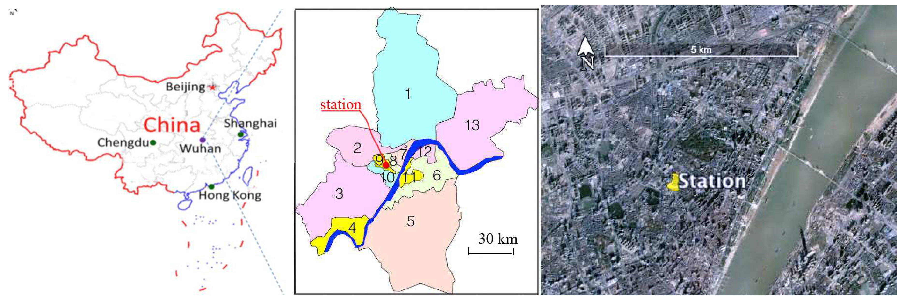
2.1. Measurement Site and Instrumentations

Wuhan city, situated in the Eastern part of the Jianghan Plain and at the intersection of the Yangtze and Hanjiang Rivers, is the largest metropolis in central China with an area of about 8500 km2 and a population of approximately 10.2 million [34]. The economic growth of Wuhan in recent years is dramatic. In 2017, Wuhan’s gross domestic product amounted to 1340 billion yuan, ranking eighth in the country, where automobile, electronic information, equipment manufacturing, food and tobacco, and energy and environmental protection are the pillar industries with economic product over one-hundred-billion Yuan (RMB). The number of vehicles in Wuhan exceeded 1,000,000 in 2010, and increased by 399,500, 414,000, and 362,000 vehicles from 2015 to 2017 respectively, and reached 2,830,000 vehicles in 2018 [36].
A typical subtropical humid monsoon climate occurs in this region with habitual climate characteristics of a hot summer and cold-humid winter. The measurement site is located at the super monitoring station of Wuhan (30°36′ N, 114°17′ E), in a typical residential area in the urban area (Figure 1). The measurement period was from 10 May to 31 May 2014. Given the springtime period, the average temperature was 25 °C within the range of 17 to 34 °C, so that there are very few usages of domestic heating and cooling with air conditioning compared to winter and summer. The average wind speed was 1.3 m/s, with north/northwest as the prevailing wind direction. Low wind speeds occurred for 24% of the recorded hours of the measurement period.
The environmental monitoring center (EMC) of Wuhan municipality has started an investigation of VOC emission inventory. However, quantitative emission inventory data is currently lacking and only the number of companies active in different industrial sectors and located in the 13 districts of Wuhan is available. This piece of information can only provide an idea of the spatial distribution of industrial sources related to VOC emission. As reported in Table 1, 562 companies have been registered, mostly for packaging and printing (165), automotive (92), and equipment and furniture manufacturing (68). The districts of Huangpi, Dongxihu, and Jingkai (numbered 1, 2, and 4 in the right graph of Figure 1, respectively) are located north, northwest, and southwest of the monitoring site, respectively, and have the largest numbers of companies. However, a rather high number of companies are also located in the districts of Jianghan and Hanyang (numbered 8 and 10 in Figure 1), much closer to the monitoring site.
VOC concentrations in ambient air have been measured by the online monitor TH-PKU 300B [37], which obtained continuous and more intensive concentrations compared to passive samplers [38]. The capture and concentration of all kinds of VOC in air is elucidated by an ultra-low temperature (−160 °C) air tube capture and concentration technology. Sampling was performed under 10 min/h, using a metal tube with a 1μm filter. Gas chromatography/mass spectrometry (GC/MS) analysis was performed using Agilent 7820 and Agilent 5975 devices. The flame ionization detector (FID) was used, and the columns were PLOT and DB-624 for MS. The temperature increased from 35 °C to 180 °C at a rate of 6 °C/min. The calibration of sampling flow rate, mass spectrometer tuning, blank experiment, and instrument calibration was conducted regularly to validate the data quality acquired by the TH-PKU 300B system. The measurement was operated by specialists from Wuhan EMC. The main calibration methods were internal standard and external standard. The internal standard at 4 ppb for each hour was inserted into the sample and analyzed together with the samples. The external standard at 4 ppb was tested once a day for all 103 species. The detection limit of 97% of the species was less than 0.05 ppb, and the detection limit of 70% of the species was less than 0.01 ppb. The measurement accuracy of 80% of the species was less than 10%, and the measurement accuracy of 45% of the species was less than 5%. The precision of 80% of the species was within ±20%, and of 60% of the species was within ±10%. Overall, 57 non-methane hydrocarbons (NMHCs), 33 halocarbons, and 13 carbonyls have been analyzed at one hour time resolution (Table 2).

2.2. Positive Matrix Factorization

Positive matrix factorization (PMF) is a multivariate factor analysis technique used for source identification and source apportionment of atmospheric pollutants. The PMF model is one of the multivariate receptor models developed by the US environmental protection agency (US-EPA). The PMF receptor model is most preferred [39] and has been widely used for source apportionment [40,41] since it simply requires measured concentration data other than a detailed and prior knowledge of sources.
In the PMF model, any data matrix X (n × m) can be factorized in two matrices G (n × p) and F (p × m); the residual matrix E as described in Equation (1).
X = G F + E      or      x i , j = k = 1 p g i , k f k , i + e i , j
where n and m are the number of samples and the number of species and p is the number of factors extracted. Equation (1) explains the case of source apportionment of atmospheric pollutants, where xi,j is the concentration of species j measured in sample i, p is the number of the factors contributing to the samples, gi,k the relative contribution of factor k to sample i, fk,j is the concentration of species j in factor profile k, and ei,j is the error of the PMF model for the j species measured in sample i. The goal is to find the gi,k, fk,j, and p values that best reproduce the observations xi,j. In the computational process the values of gi,k and fk,j are adjusted until a minimum value of the objective function Q for a given p is found, where Q is defined in Equation (2):
Q = j = 1 m i = 1 n e i , j s i , j 2
where si,j is the uncertainty of the concentration of species j in sample i, n is the number of samples and m the number of species.
Different from other receptor models (i.e., chemical mass balance), the PMF solves Equation (1) without requiring prior knowledge of the number and type of sources that contribute to the chemical characteristics of the samples. Simply relying on two input files, sample species’ concentration data and sample species’ uncertainty data, the PMF solves the equation for each factor p, concurrently estimating the factor contributions (G) and the factor profiles (F). Sample species uncertainty can be derived from actual uncertainty data of analytical determination or be estimated through an equation-based approach from specific parameters, such as the detection limit (DL) of the measurement method [42,43,44].
In this study, 63 significant species of the measured 103 VOCs were selected for the PMF 5.0 model runs (Table 2). Following the recommendations of the PMF user guide [45], the missing concentration data in the time series of selected species have been replaced with the median values of the data distributions, while the related value of the uncertainty was set as equal to four times the median. The uncertainty determination was followed the description by Polissar et al. [42] and Yuan et al. [46]. Outliers (values higher than 5% of all samples) were excluded from the dataset and flagged as a missing value. Concentrations less than or equal to the instrumental detection limit have been substituted by half the DL and the corresponding uncertainty was set as two times the DL. The uncertainty of each species is determined using Equation (3):
U i , j = 0.05 c i , j + 0.05 i c i , j / i
where Ui,j is the uncertainty for the sample i and species j, while ci,j is the concentration of the species j in the sample i.

Method for Selection of Factor Number

The final goal of the PMF runs is the determination of the number of factors, where factors refer to the sources of emission, the chemical composition of each factor, and the contribution of each factor to the sample minimizing the residuals. In general, source apportionment techniques do not recognize a single source but rather source categories, for instance traffic exhaust, biomass burning, whose emissions are characterized by specific markers in their chemical composition profiles.
As the PMF solution depends on the number of factors used to initialize the model run, this choice strongly affects source apportionment analysis. Additionally, the factors resulting from PMF have to be associated with emission sources characterized by the related chemical compositions. In general, increasing the number of factors would decrease the error of estimated concentrations, thus the higher the number of factors the better the explanation of observed concentration data but, at the same time, the more difficulty for the association of each factor to a corresponding proper source. Emission inventory data may be useful to address the choice of the number of factors. In our case, however, quantitative estimation of VOC emissions was not available and the suggestion about the wide variety of industrial activities potentially responsible for VOC emissions was the only available information. Thus, in order to make the choice of the number of factors as less arbitrarily as possible, we developed a multiple-indicator approach based on the values of three different statistical indicators for PMF model performance: (i) the correlation coefficients between observed and model reconstructed concentrations for a single VOC; (ii) an overall correlation coefficient for all the VOCs considered in PMF runs; and (iii) the normalized absolute error between observed and reconstructed concentrations for the entire VOCs dataset.
The first indicator is intended to assess the PMF performance by properly reconstructing the observed time trend of a single VOC species. Practically, we set a minimum threshold value (r2min = 0.8) for the correlation coefficient between observed and reconstructed concentrations and counted the number of species (Np) with an actual coefficient (r2act,p) greater than that for each model run. An increasing number Np of species with r2act,p > r2min is expected as PMF model runs are initialized with an increasing number or factors p.
The second indicator, instead of considering r2act,p values for a single VOC, relies on a weighted average correlation coefficient r2avg,p calculated with Equation (4):
r avg , p 2 = j ( r act , p , j 2 C a v g , i j C a v g , i )
where r2act,p,j is the coefficient of correlation between observed and reconstructed concentrations for species j resulting from a PMF run with p factors, Cavg,j the average concentration of the species j, and N the number of species considered in PMF runs (N = 63 in this study). This indicator is intended to assess overall PMF performance in reconstructing the time patterns of the entire VOC dataset, giving larger relative importance to the most abundant species through concentration-based weight. As for the first indicator, larger values of r2avg,p are expected in PMF runs initialized with larger number of factors.
The third indicator, intended to assess the accuracy in the model reconstruction of the observed concentration values for the entire dataset, is the normalized absolute error (NAEp) calculated according to Equation (5):
N A E p = i | C o b s , i C p r e d , i , p | C o b s , i
where Cobs,i is the observed concentration of specie i and Cpred,i is the corresponding reconstructed concentrations by PMF model with p factors. Contrary to the two previous indicators, NAEp is expected to decrease as p increases because of the enhanced ability of the model in data reconstruction.
Performing different PMF simulations, initialized with increasing number of factors p (in our case we considered p = 4, 5, 6, 7, and 8) leads to a set of p-dependent indicators (Np, r2avg,p, and NAEp) that account for both the time pattern reproduction and modeled concentration accuracy. The comparative analysis of the behavior of the indicator sets in relation to the number of factors and, in particular, a marginal improvement in data reconstruction for increasing number of factors, addresses the selection of a proper number of factors (i.e., of sources), is acceptable both as a mathematical solution but, most of all, is reasonable for the environmental interpretation of the results (i.e., source identification).

3. Results and Discussions

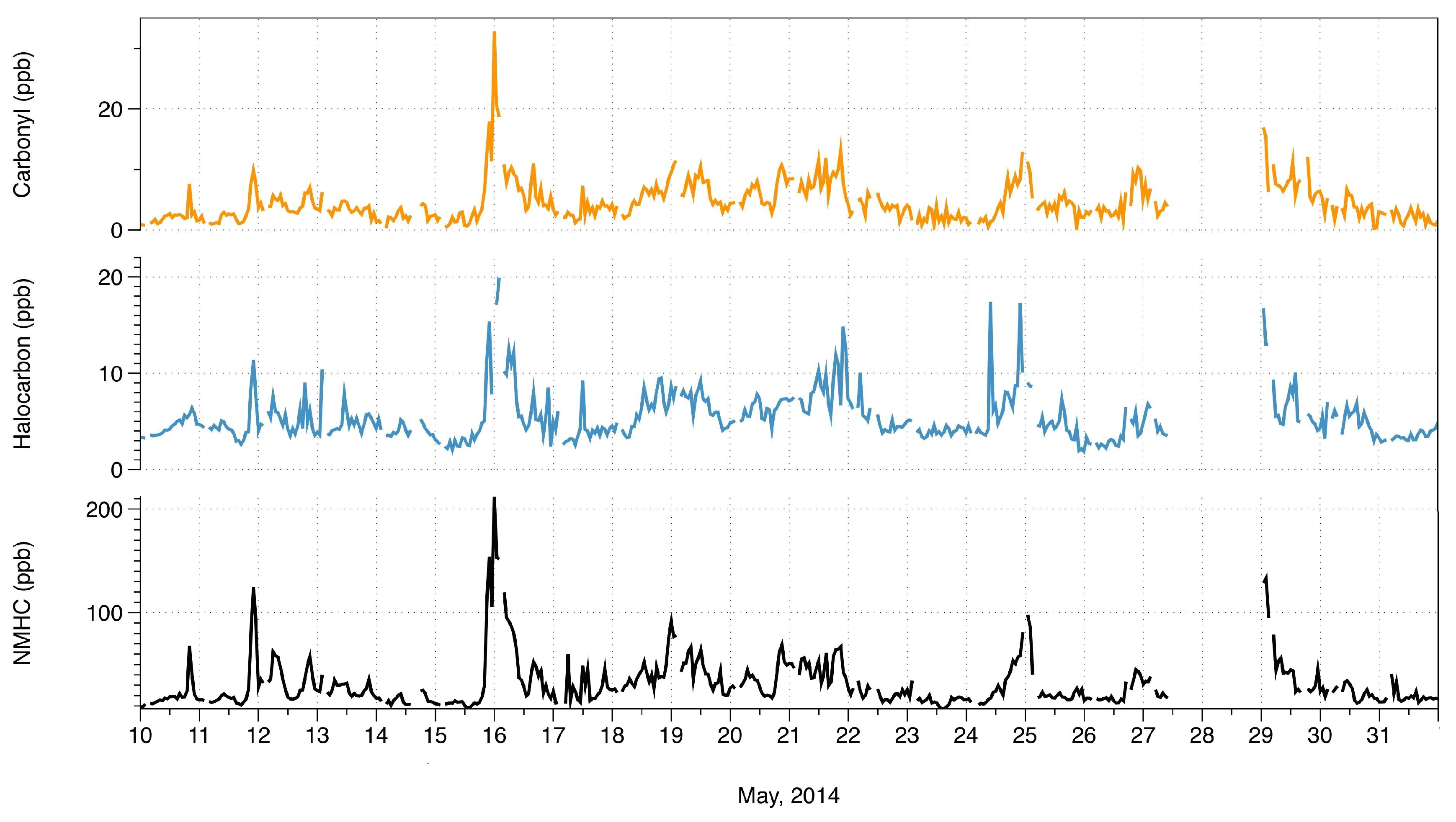
3.1. General Pattern of VOC Concentrations

The time pattern of NMHC, halocarbon, and carbonyl concentrations observed during the monitoring period in Wuhan is presented in Figure 2.
In general, the concentration of NMHCs is about one order of magnitude higher than the halocarbons and carbonyls. The average concentration of NMHCs was 31 ppb. Halocarbons and carbonyls concentrations were in the order of a few tenths of ppb but mostly below 20 ppb. The average concentration of the halocarbons was 5.4 ppb. The average concentration of carbonyls was 4.5 ppb. Concentrations of NMHCs, halocarbons, and carbonyls show peaks around the 16th and 25th, these are influenced by local weather type and more pronounced than the diurnal effect (see Figure 2). During the period of 16 to 25 May, the atmosphere was controlled by subtropical high pressure and, at local scale there appeared strong straight air [47], thus local emissions accumulated which resulted in a notable increase of all three groups.
The most abundant VOCs during the monitoring period were the lightest alkanes and alkenes (ethane, propane, n-butane, and ethylene) together with acetylene and the lightest, single-ring aromatics (benzene and toluene), which had period-averaged concentrations in the 1–5 ppb range. Table 3 reports the comparison of these VOCs from Wuhan with literature data reported in other works from urban areas in China or other countries. Even though the reported concentration levels depend on several factors (i.e., monitoring season, monitoring site location, and exposure to emission sources and analytical methods) [48], they allow for contextualization of Wuhan data, showing substantial agreement with those from other Chinese cities. In particular, the comparison shows that the concentration levels of benzene and toluene in Wuhan are similar to those concurrently measured in Beijing in the same period of May 2014.

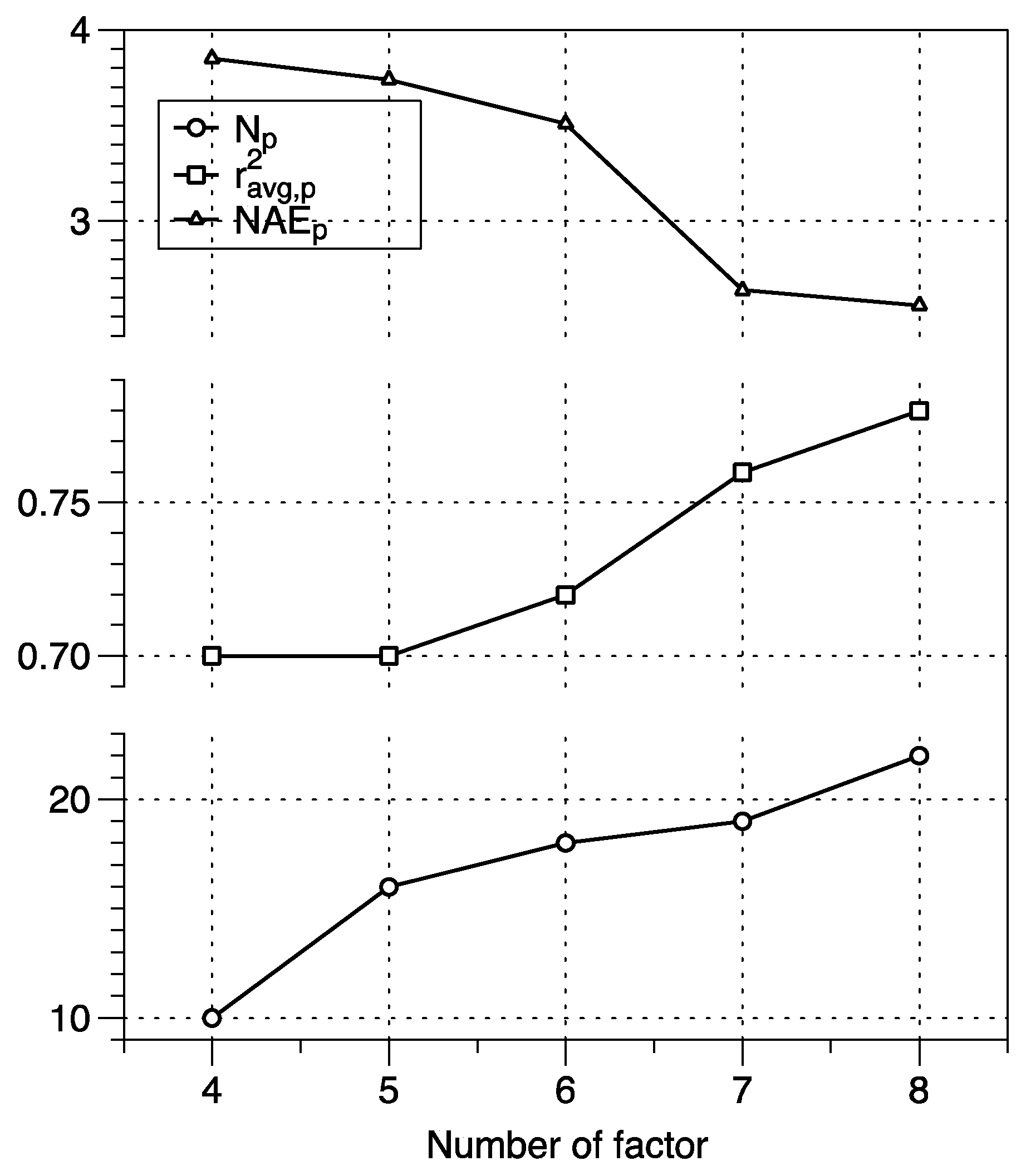
3.2. Factor Selection for PMF Runs

Figure 3 shows the results for the sets of the three statistical indicators obtained by PMF simulations initialized with four, five, six, seven, and eight factors, respectively.
The minimum of Np with correlation coefficients greater than the threshold (r2min = 0.8) is N4 = 10, which is obtained with a 4-factor simulation; the maximum number of Np is N8 =22, which is obtained with an 8-factor simulation (Figure 3, bottom panel). As expected, Np becomes larger as p increases but the trend is not linear. The transition from four to five factors leads to a sharp increase in Np (from 10 to 16), whereas, further increase of the number of factors results is a more regular increase of the Np. Actually, passing from six to seven factors we have an increase of one unit for Np (18 to 19), while going from 7 up to 8 factors Np varies from 19 to 22.
The weighted average correlation coefficient r2avg,p ranges between 0.70 and 0.78 (Figure 4, middle panel) with an increasing trend for Np. However, the transition from 4 to 5 factors does not imply any significant change in the indicator (r2avg,4 ≈ r2avg,5), whose notable increase occurs only when shifting from 6 (r2avg,6 = 0.72) to 7 (r2avg,7 = 0.76) factors. One additional factor included in PMF simulation leads to a small increase for the indicator value (from 0.76 up to 0.78).
Contrary to the previous indicators, the NAEp shows a declining trend for increasing number of factors (Figure 3, top panel) down from NAE4 = 3.85 to NAE8 = 2.56. However, while PMF-increased accuracy is rather limited from four to six factors, a clear improvement is obtained when shifting from six to seven factors, with NAEp passing from NAE6 = 3.51 to NAE7 = 2.64 (−25%); conversely, shifting from seven up to eight factors does not involve important improvement (NAE8 = 2.56, that is only 3% less than NAE7).
The comparative analysis of the behavior of the indicators in relation to the number of factors supports that the 7-factor solution is mathematically reasonable. Too few factors may lead to an underestimation of the emission in spring in the area, additionally, if there are too many factors, this can prevent correct identification of sources, so our final choice fell on the 7-factor solution.

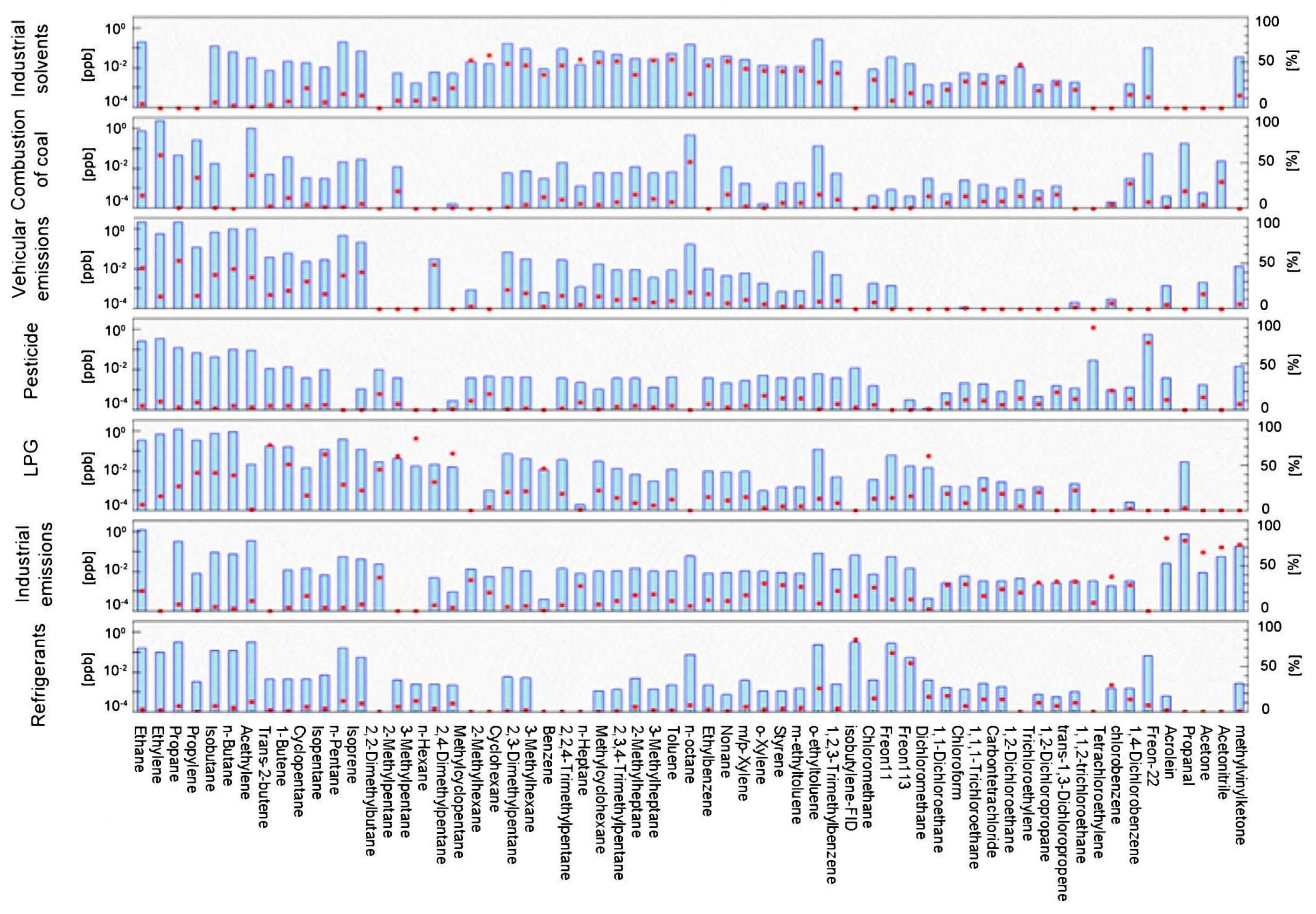
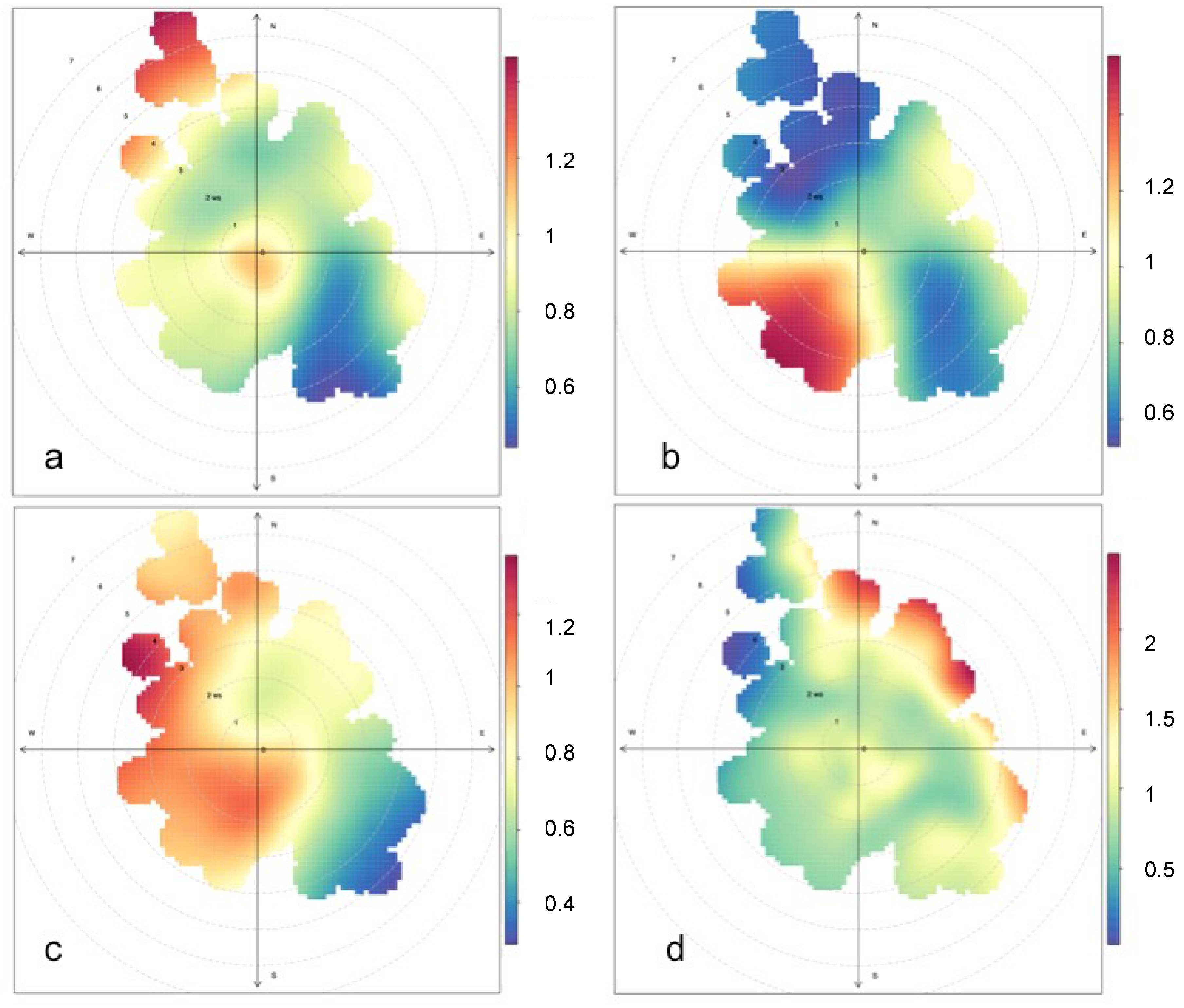
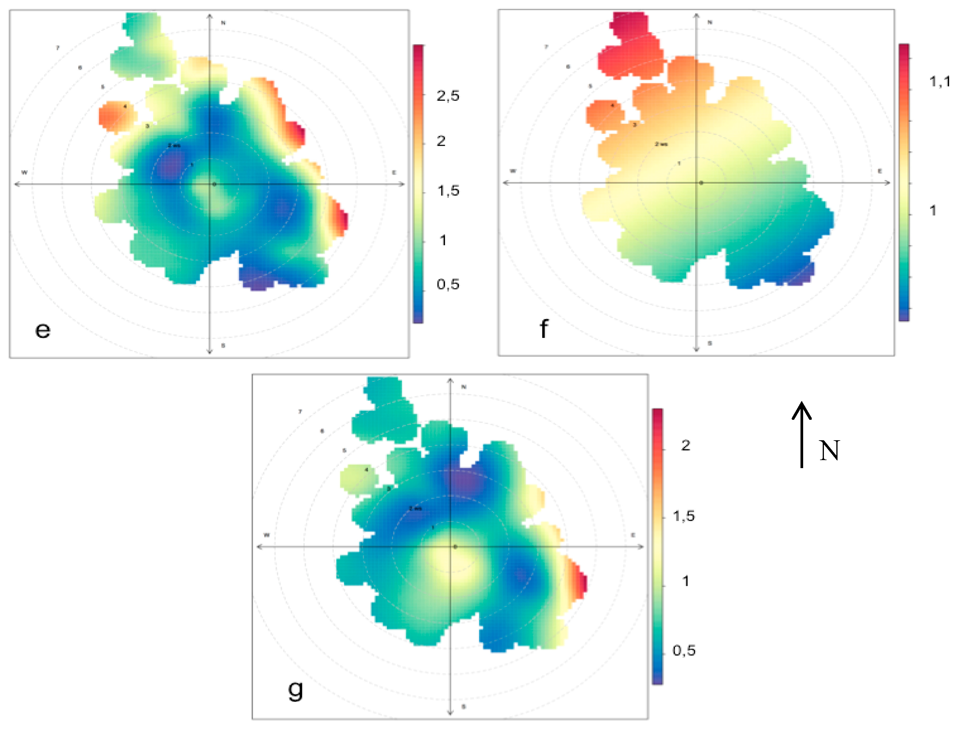
3.3. Source Identification by PMF

The profiles of the factors resulting from the 7-factor solution are shown in Figure 4. The concentration of each species is divided into each factor and indicated by a blue color, and the percentage that each species is explained by the factor is indicated by a red square. The concentrations corresponding to the y axis on the left are expressed in the logarithmic scale and the percentage of species explained by the factor must be sought in the y axis on the right. The seven factors have been identified as sources of VOCs on the basis of the resulting emission profile markers explained below.
The first factor is assigned to industrial use of solvents. This factor explains the presence of TEX (toluene 15.4%, ethylbenzene 51.6%, and xylene 40.2%) as well as C6 and C7 alkanes (cyclohexane 49%, methylcyclopentane 51.7%, 2-methylpentane 51.9%, and 3-methylpentane 53.3%). All these organic compounds are commonly used as solvents in industrial processes [32,46]. The main industrial sources of VOCs present in Wuhan are from the manufacture of cars, press, production of furniture, and production of shoes and toys. VOCs explained by this factor are mainly related to paints and use of adhesives in the production processes [46].
The second factor explains mainly ethylene (58.6%) and toluene (52.0%), which are associated with the combustion of coal [32,46,53]. In China, coal is the dominant source of energy [54]. Coal combustion is also an important VOCs source [55].
The third factor is associated with the exhaust gases of motor vehicles, identified by specific tracers such as ethylene, toluene, benzene, acetylene, and other aromatics and alkanes (propane, n-butane etc.) [56]. This source, identified as vehicular emissions, explains 14.1% of ethylene, 53.7% of propane, and 35.4% of acetylene. These VOCs, indicated as tracers of emissions from vehicles, are consistent with other PMF-based studies for Los Angeles [53], Shanghai [57], Tianjin [58], Houston [59], and other receptor models, such as in Turkey reported by Dumanoglu et al. [25].
The fourth factor is characterized by the dominant presence of two specific VOCs, trans-1,3-dichloropropane (90.8%) and 1,4-dichlorobenzene (73.7%). These two species are part of the family of chlorinated VOCs and are commonly used as pesticides.
The fifth factor explains n-butane (39.4%), trans-2-butene (72.5%), and 1-butene (50.7%). The combination of these species is typically found in the combustion gas of liquefied petroleum gas (LPG) [59], as also reported in other works in China [46,57]. Actually, in Wuhan there are no vehicles using LPG, but LPG is used in catering for domestic use is very popular in urban areas [32].
The sixth factor is associated with industrial emissions, because it explains the high attendance of Freon 22 (81.0%), acrolein (77.7%), acetonitrile (70.5%), and methylvinylketone (73.3%). Freon 22 has been commonly used as a fuel, coolant, and as a versatile intermediate in the chemical industries. Acrolein is used in manufacturing plastics and synthetic rubber, and is an important and versatile intermediate for the chemical industry [49]. Acetonitrile is an important solvent in the chemical industries [60], and with the increase of its wide use in the industrial sector such as pharmaceuticals, solvents, and chromatography, the public is paying more and more attention to its environmental presence [61]. Methylvinylketone is used as a chemical reagent.
The seventh factor is associated with the use of refrigerants as it explains the presence of Freon 11 (53.9%), the first cooling fluid of wide use, and of chloromethane (64.8%) that, in the past, has been used widely as a coolant. Given the risks related to its contribution to climate change and ozone depletion, its use was reduced in most countries but it is still determinable in Wuhan as a source contributor. There could be some emission and it might not be due to the residual of its long-life time.
The contributions of the emission sources to the observed VOC concentrations were also calculated. The primary source is vehicular emissions (45.4%), which is comparable to that in PRD (~50%) [13] and Beijing (57.7%) [62], and was over 40% in a French urban area ten years ago [30]. Other dominating sources are industrial emissions (22.5%) and the combustion of coal (14.7%). Other sources that contribute less than 10% include LPG combustion (9.7%), industrial solvents (4.4%), and pesticide use (3.3%). The contribution from the use of refrigerants is less than 0.05%, but it is worth noting because of the high toxicity risks associated with compounds emitted by this source. Lyu et al. [32] conducted measurement for all four seasons (February 2013 to October 2014) and found that vehicular exhausts (27.8 ± 0.9%), coal burning (21.8 ± 0.8%) and LPG had (19.8 ± 0.9%) were the main contributors to VOCs in Wuhan; industrial solvents and pesticide use were not reported.
The results of the source apportionment were represented using polar plots that show the association between the contribution of the sources generated by PMF and the origin of the air masses [63]. The results are graphically displayed in the panels of Figure 5, with computed source contributions in color scale as a function of wind speed and wind direction on an hourly basis.
The sources identified as being associated with the industrial use of solvents and industrial emissions gave their largest contributions when winds blow from the north northwest and northwest with respect to the location of data collection, with wind speeds ranging from 5 to 7 m/s (Figure 5a,f). The source associated with the combustion of coal (Figure 5b) occurs in a confined zone of wind directions between west southwest and south southwest and is associated with lower wind speeds.
The source identified as vehicular emissions (Figure 5c) is associated with westerly winds and is spread around the monitoring station mainly from south to west northwest, but also up to the north. In the area west of the monitoring site we can find a dense road system accounting for a high mileage of the Wuhan road network, including two high-capacity ring roads. The association of the largest contributions of this source with rather low wind speeds confirms the very local origin of the traffic source.
Figure 5d shows that the area in which the source of pesticides has a greater contribution is located to the northeast of the monitoring site, particularly where the wind is approximately 4 m/s. There is the same origin as the LPG source (Figure 5e). The cooling source (Figure 5g) provides the lowest contribution among those sources to Wuhan; it is more pronounced in west south.

4. Conclusions

In this study, a multiple-indicator method, based on the marginal improvement in data reconstruction for an increasing number of factors initializing PMF runs, has been developed to select the proper number of factors. The emission sources of VOCs in the biggest city in Central China, Wuhan, have been investigated using the positive matrix factorization (PMF) model.
This method suggested a 7-factor PMF solution; seven sources could be associated with emission sources based on the results of VOC source profiles. The identified seven sources are vehicular emissions (45.4%), industrial emissions (22.5%), combustion of coal (14.7%), LPG combustion (9.7%), industrial use of solvents (4.4%), pesticides (3.3%), and use of refrigerants. The vehicular emissions source profile shows high attendance of ethylene, toluene, benzene, acetylene and other aromatics, and alkanes, which are typical VOCs emitted from the exhaust gases of motor vehicles. The industrial emissions source profile shows high contribution of Freon 22, acrolein, acetonitrile, and methylvinylketone, all typical intermediate products and process materials in the chemical industry. The profile of the combustion of coal source is characterized by the strong presence of ethylene and toluene, whereas butane and butene characterize the profile of the LPG combustion source, mainly related to catering for domestic use, which is very popular in Wuhan city.
The origins of the sources identified by PMF are conducted in PolarPlot. The results indicate that the sources identified as industrial solvents and industrial emissions dominate in the area between the north northwest and northwest. The source associated with the combustion of coal is very limited in the zone between west southwest and south southwest of the monitoring station. The source associated with the vehicular emission is spread around the point contribution monitoring but with a predominant component of the sources of pesticides and liquefied petroleum gas more associated with winds from east of the monitoring site. These findings can be used to track the source origins for the development of an emission reduction strategy in Wuhan and can implement this method in other cities suffering from air pollution.
The new developed multiple-indicator method is independent from the type and number of species put in PMF model. Each of the indicators provides robust values to compare, which will minimize the influence caused by experience on source apportionment of users. The method was developed specially for the increased demand of VOC source identification in China, but it can be used for any kind of species source apportionment analysis by PMF model.

Author Contributions

F.W. and G.L. conceived and designed the experiments; Z.Z. (Zhangxiong Zhong) and C.A. performed the experiments; C.A., Z.Z. (Zhenyi Zhang) and F.W. analyzed the data; Z.H. contributed materials; F.W., C.A. and Z.Z. (Zhenyi Zhang) wrote the paper. G.L. contributed analysis tools and provided discussion and comments on the paper.

Funding

We would like to thank the National Key Research and Development Program (2017YFA0605002) for their financial support as well as the Politecnico di Milano international fellowship grant.

Acknowledgments

We acknowledge the authors of the open source R program (R Core Team, 2015).

Conflicts of Interest

The authors declare no conflict of interest.

References

  1. Aikin, A.C.; Herman, J.R.; Maier, F.J.; McQuillan, C.J. Atmospheric chemistry of ethane and ethylene. J. Geophys. Res. Oceans Atmos. 1982, 87, 3105–3118. [Google Scholar] [CrossRef]
  2. Tancrede, M.; Wilson, R.; Zeise, L.; Crouch, E.A.C. The carcinogenic risk of some organic vapours indoors: A theoretical survey. Atmos. Environ. 1987, 21, 2187–2193. [Google Scholar] [CrossRef]
  3. Son, Y.S.; Kim, J.C. Decomposition of sulfur compounds by radiolysis: I. Influential factors. Chem. Eng. J. 2015, 262, 217–223. [Google Scholar] [CrossRef]
  4. Massolo, L.; Rehwagen, M.; Porta, A.; Ronco, A.; Herbarth, O.; Mueller, A. Indoor-outdoor distribution and risk assesment of volatile organic compounds in the atmosphere of industrial and urban areas. Environ. Toxicol. 2010, 25, 339–349. [Google Scholar] [CrossRef] [PubMed]
  5. Sweet, C.W.; Vermette, S.J. Toxic volatile organic compounds in urban air Illinois. Environ. Sci. Technol. 1992, 26, 165–173. [Google Scholar] [CrossRef]
  6. Bari, M.A.; Kindziersk, W.B. Ambient volatile organic compounds (VOCs) in Calgary, Alberta: Sources and screening health risk assessment. Sci. Total Environ. 2018, 631–632, 627–640. [Google Scholar] [CrossRef] [PubMed]
  7. He, J.; Gong, S.; Yu, Y.; Yu, L.; Wu, L.; Mao, H.; Song, C.; Zhao, S.; Liu, H.; Li, X.; Li, R. Air pollution characteristics and their relation to meteorological conditions during 2014–2015 in major Chinese cities. Environ. Pollut. 2017, 223, 484–496. [Google Scholar] [CrossRef] [PubMed]
  8. Zhang, Y.; Hong, R.; Fu, H.; Zhou, D.; Chen, J. Observation and analysis of atmospheric volatile organic compounds in a typical petrochemical area in Yangtze River Delta, China. J. Environ. Sci. 2018, in press. [Google Scholar] [CrossRef] [PubMed]
  9. Liu, B.; Liang, D.; Yang, J.; Dai, Q.; Bi, X.; Feng, Y.; Yuan, J.; Xiao, Z.; Zhang, Y.; Xu, H. Characterization and source apportionment of volatile organic compounds based on 1-year of observational data in Tianjin, China. Environ. Pollut. 2016, 218, 757–769. [Google Scholar] [CrossRef] [PubMed]
  10. Li, L.; Xie, S.; Zeng, L.; Wu, R.; Li, J. Characteristics of volatile organic compounds and their role in ground-level ozone formation in the Beijing-Tianjin-Hebei region,China. Atmos. Environ. 2015, 113, 247–254. [Google Scholar] [CrossRef]
  11. Li, J.; Xie, S.; Zeng, L.; Li, L.; Li, Y.; Wu, R. Characterization of ambient volatile organic compounds and their sources in Beijing, before, during, and after Asia-Pacific Economic Cooperation China 2014. Atmos. Chem. Phys. 2015, 15, 7945–7959. [Google Scholar] [CrossRef]
  12. An, J.; Zhu, B.; Wang, H.; Li, Y.; Lin, X.; Yang, H. Characteristics and source apportionment of VOCs measured in an industrial area of Nanjing, Yangtze River Delta, China. Atmos. Environ. 2014, 97, 206–214. [Google Scholar] [CrossRef]
  13. Liu, Y.; Shao, M.; Lu, S.; Chang, C.; Wang, J.; Chen, G. Volatile organic compound (VOC) measurements in the Pearl River Delta (PRD) region, China. Atmos. Phys. Chem. 2008, 8, 1531–1545. [Google Scholar] [CrossRef]
  14. Guo, H.; Ling, Z.H.; Cheng, H.; Simpson, I.; Lyu, X.; Wang, X.; Shao, M.; Lu, H.; Blake, D. Tropospheric volatile organic compounds in China. Sci. Total Environ. 2017, 574, 1021–1043. [Google Scholar] [CrossRef] [PubMed]
  15. Klimont, Z.; Streets, D.G.; Gupta, S.; Cofala, J.; Fu, L.X.; Ichikawa, Y. Anthropogenic emissions of non-methane volatile organic compounds in China. Atmos. Environ. 2002, 36, 1309–1322. [Google Scholar] [CrossRef]
  16. Saeaw, N.; Thepanondh, S. Source apportionment analysis of airborne VOCs using positive matrix factorization in industrial and urban areas in Thailand. Atmos. Pollut. Res. 2015, 6, 644–650. [Google Scholar] [CrossRef]
  17. Li, B.; Sai, S.; Yong, H.; Xue, G.; Huang, Y.; Wang, L.; Cheng, Y.; Dai, W.; Zhong, H.; Cao, J.; Lee, S. Characterizations of volatile organic compounds (VOCs) from vehicular emissions at roadside environment: The first comprehensive study in Northwestern China. Atmos. Environ. 2017, 161, 1–12. [Google Scholar] [CrossRef]
  18. Wang, H.; Jing, S.; Lou, S.; Hu, Q.; Li, T.; Shi, K.; Cheng, Q.; Li, P.; Chen, C. Volatile organic compounds (VOCs) source profiles of on-road vehicle emissions in China. Sci. Total Environ. 2017, 607–608, 253–261. [Google Scholar]
  19. MEP, China. The Technical Guide for the Compilation of Emission Inventory of Volatile Organic Compounds. 2014; (in Chinese). Available online: http://hbj.neijiang.gov.cn/2016/12/1282079.html (accessed on 10 July 2018).
  20. Wang, Q.; Li, S.; Dong, M.; Li, W.; Gao, X.; Ye, R.; Zhang, D. VOCs emission characteristics and priority control analysis based on VOCs emission inventories and ozone formation potentials in Zhoushan. Atmos. Environ. 2018, 182, 234–241. [Google Scholar] [CrossRef]
  21. Shen, L.; Xiang, P.; Liang, S.; Chen, W.; Wang, M.; Lu, S.; Wang, Z. Sources Profiles of Volatile Organic Compounds (VOCs) Measured in a Typical Industrial Process in Wuhan, Central China. Atmosphere 2018, 9, 297. [Google Scholar] [CrossRef]
  22. Ou, J.; Zheng, J.; Yuan, Z.; Guan, D.; Huang, Z.; Yu, F.; Shao, M.; Louie, P. Reconciling discrepancies in the source characterization of VOCs between emission inventories and receptor modeling. Sci. Total Environ. 2018, 628-629, 697–706. [Google Scholar] [CrossRef] [PubMed]
  23. Leuchener, M.; Rappengluck, B. VOC source-receptor relationships in Houston during TexAQS-II. Atmos. Environ. 2010, 44, 4056–4067. [Google Scholar] [CrossRef]
  24. Song, Y.; Dai, W.; Shao, M.; Liu, S.; Lu, W.; Kuster, P. Goldan Comparison of receptor models for source apportionment of volatile organic compounds in Beijing, China. Environ. Pollut. 2008, 156, 174–183. [Google Scholar] [CrossRef] [PubMed]
  25. Dumanoglu, Y.; Kara, M.; Altiok, H.; Odabasi, M.; Elbir, T.; Bayram, A. Spatial and seasonal variation and source apportionment of volatile organic compounds (VOCs) in a heavily industrialized region. Atmos. Environ. 2014, 98, 168–178. [Google Scholar] [CrossRef]
  26. Li, J.; Zhai, C.; Yu, J.; Liu, R.; Li, Y.; Zeng, L.; Xie, S. Spatiotemporal variations of ambient volatile organic compounds and their sources in Chongqing, a mountainous megacity in China. Sci. Total Environ. 2018, 627, 1442–1452. [Google Scholar] [CrossRef]
  27. Zhu, H.; Wang, H.; Jiang, S.; Wang, Y.; Cheng, T.; Tao, S.; Lou, S.; Qiao, L.; Chen, J. Characteristics and sources of atmospheric volatile organic compounds (VOCs) along the mid-lower Yangtze River in China. Atmos. Environ. 2018, 190, 232–240. [Google Scholar] [CrossRef]
  28. Paatero, P.; Tapper, U. Positive matrix factorization: A non-negative factor model with optimal utilization of error estimates of data values. Environmetrics 1994, 5, 111–126. [Google Scholar] [CrossRef]
  29. Badol, C.; Locoge, N.; Galloo, J. Using a source-receptor approach to characterise VOC behaviour in a French urban area influenced by industrial emissions: Part II: Source contribution assessment using the Chemical Mass Balance (CMB) model. Sci. Total Environ. 2008, 389, 429–440. [Google Scholar] [CrossRef] [PubMed]
  30. Zheng, J.; Shao, M.; Che, W.; Zhang, L.; Zhong, L.; Zhang, Y.; Streets, D. Speciated VOC emission inventory and spatial patterns of ozone formation potential in the Pearl River Delta, China. Environ. Sci. Technol. 2009, 43, 8580–8586. [Google Scholar] [CrossRef] [PubMed]
  31. Wang, G.; Chen, S.; Wei, W.; Zhou, Y.; Yao, S.; Zhang, H. Characteristics and source apportionment of VOCs in the suburban area of Beijing, China. Atmos. Pollut. Res. 2016, 4, 711–724. [Google Scholar] [CrossRef]
  32. Lyu, X.P.; Chen, N.; Guo, H.; Zhang, W.H.; Wang, N.; Wang, Y.; Liu, M. Ambient volatile organic compounds and their effect on ozone production in Wuhan, central. Sci. Total Environ. 2016, 541, 200–209. [Google Scholar] [CrossRef] [PubMed]
  33. Cheng, H.; Gong, W.; Wang, Z.; Zhang, F.; Wang, X.; Lv, X.; Liu, J.; Fu, X.; Zhang, G. Ionic composition of submicron particles (PM1.0) during the long-lasting haze period in January 2013 in Wuhan, central China. J. Environ. Sci. 2014, 26, 810–817. [Google Scholar] [CrossRef]
  34. Zhang, F.; Wang, Z.; Cheng, H.; Lv, X.; Gong, W.; Wang, X.; Zhang, G. Seasonal variations and chemical characteristics of PM2.5 in Wuhan, central China. Sci. Total Environ. 2015, 518–519, 97–105. [Google Scholar] [CrossRef] [PubMed]
  35. Zeng, P.; Lyu, X.P.; Guo, H.; Zhang, W.; Wang, N.; Wang, Y.; Liu, M. Causes of ozone pollution in summer in Wuhan, Central China. Environ. Pollut. 2018, 241, 852–861. [Google Scholar] [CrossRef] [PubMed]
  36. Hubei statistical bureau, 2017 Hubei statistical yearbook. 2018. Available online: http://www.yearbookchina.com (accessed on 23 September 2018).
  37. Tianhong Instrument Group. TH-300B Atmosphere Volatile Organic Compounds (VOC) Rapid and Continuous Automatic Monitoring System. 2012. Available online: https://www.instrument.com.cn/netshow/SH101607/C164305.htm (accessed on 10 July 2018).
  38. Huang, C.; Shan, W.; Xiao, H. Recent Advances in Passive Air Sampling of Volatile Organic Compounds. Aerosol Air Qual. Res. 2018, 18, 602–622. [Google Scholar] [CrossRef] [Green Version]
  39. Khan, M.; Latif, M.; Lim, C.; Amil, N.; Jaafar, S.; Dominick, D.; Nadzir, M.; Sahan, M.; Tahir, N. Saesonal effect and source apportionment of polycyclic aromatic hydrocarbons in PM2.5. Atmos. Environ. 2015, 106, 178–190. [Google Scholar] [CrossRef]
  40. Yu, L.; Wang, G.; Zhang, R.; Zhang, L.; Song, Y.; Wu, B.; Wu, X. Characterization and Source Apportionment of PM2.5 in a urban environment in Beijing. Aerosol Air Qual. Res. 2013, 574–583. [Google Scholar] [CrossRef]
  41. Gao, J.; Tian, H.; Cheng, K. Seasonal and spatial variation of trace elements in multisize airborne particulate matters of Beijing, China: Mass concentration, enrichment characterization and source apportionment of volatile organic compounds (VOCs)in a heavily industrialized region. Atmos. Environ. 2014, 257–265. [Google Scholar] [CrossRef]
  42. Polissar, A.V.; Hopke, P.K.; Paatero, P.; Malm, W.C.; Sisler, J.F. Atmospheric aerosol over Alaska: 2. Elemental composition and sources. J. Geophys. Res. Atmos. 1998, 103, 19045–19057. [Google Scholar] [CrossRef] [Green Version]
  43. Reff, A.; Eberly, S.I.; Bhave, P.V. Receptor modeling of ambient particulate matter data using positive matrix factorization: Review of existing methods. J. Air Waste Manag. Assoc. 2007, 57, 146–154. [Google Scholar] [CrossRef]
  44. Kara, M.; Hopke, P.K.; Dumanoglu, Y.; Altiok, H.; Elbir, T.; Odabasi, M.; Bayram, A. Characterization of PM Using Multiple Site Data in a Heavily Industrialized Region of Turkey. Aerosol Air Qual. Res. 2015, 15, 11–27. [Google Scholar] [CrossRef]
  45. US-Environmental Protection Agency. EPA Positive Matrix Factorization (PMF) 5.0 Fundamentals and User Guide, EPA/600/R-14/108. 2014. Available online: www.epa.gov (accessed on 10 September 2015).
  46. Yuan, Z.; Zhong, L.; Lau, A.; Yu, J.Z.; Louie, P. Volatile organic compounds in the Pearl River Delta: Identification of source regions and recommendations for emission-oriented monitoring strategies. Atmos. Environ. 2013, 76, 162–172. [Google Scholar] [CrossRef]
  47. Wang, F.; Zhong, Z.; Wu, S.; Zhang, W.; Li, Q.; Hu, S.; Wang, J. Case study of Wuhan dust pollution in May 2014. Acta Sci. Nat. Univ. Pekinensis 2015, 51, 1132–1140. [Google Scholar]
  48. Li, L.; Chen, Y.; Zeng, L.; Shao, M.; Xie, S.; Chen, W.; Liu, S.; Wu, Y.; Cao, W. Biomass burning contribution to ambient volatile organic compounds in the Chengdu-Chongqing Region, China. Atmos. Environ. 2014, 99, 403–410. [Google Scholar] [CrossRef]
  49. Liu, L.; Ye, X.; Bozell, J. A comparative review of petroleum-based and bio-based acrolein production. ChemSusChem 2012, 6, 1162–1180. [Google Scholar] [CrossRef] [PubMed]
  50. Guo, H.; Wang, T.; Simpson, I.J.; Blake, D.R.; Yu, X.M.; Kwok, Y.H.; Li, Y.S. Source contributions to ambient VOCs and CO at a rural site in eastern China. Atmos. Environ. 2004, 38, 4551–4560. [Google Scholar] [CrossRef]
  51. Guo, H.; Wang, T.; Blake, D.; Simpson, I.; Kwok, Y.; Li, Y. Regional and local contributions to ambient non-methane volatile organic compounds at a polluted rural/coastal site in Pearl River Delta, China. Atmos. Environ. 2006, 40, 2345–2359. [Google Scholar] [CrossRef]
  52. Schneidemesser, E.; Monks, P.; Duelmer, C. Global comparison of VOC and CO observations in urban areas. Atmos. Environ. 2010, 44, 5053–5064. [Google Scholar] [CrossRef]
  53. Brown, S.G.; Frankel, A.; Hafner, H. Source Apportionment of VOCs in the Los Angeles area using positive matrix factorization. Atmos. Environ. 2007, 41, 227–237. [Google Scholar] [CrossRef]
  54. Quan, J.; Tie, X.; Zhang, Q.; liu, Q.; Li, X.; Gao, Y.; Zhao, D. Characteristics of haevy aerosol pollution during the 2012-2013 winter in Beijing, China. Atmos. Environ. 2014, 88, 83–89. [Google Scholar] [CrossRef]
  55. Wang, M.; Shao, M.; Lu, S.; Yang, Y.; Chen, W. Evidence of coal combustion contribution to ambient VOCs during winter in Beijing. Chin. Chem. Lett. 2013, 24, 829–832. [Google Scholar] [CrossRef]
  56. Watson, J.G.; Chow, J.; Fujita, E. Review of volatile organic compound source apportionment by chemical mass balance. Atmos. Environ. 2001, 35, 1567–1584. [Google Scholar] [CrossRef]
  57. Cai, C.; Geng, F.; Tie, X.; Yu, Q.; An, J. Characteristics and spource apportionment of VOCs measured in Shanghai, China. Atmos. Environ. 2010, 44, 5005–5014. [Google Scholar] [CrossRef]
  58. Han, M.; lu, X.; Zhao, C.; Ran, L.; Han, S. Characterization and Source Apportionment of Volatile Organic Compounds in urban and suburban Tianjin, China. Adv. Atmos. Sci. 2015, 32, 439–444. [Google Scholar] [CrossRef]
  59. Leuchner, M.; Gubo, S.; Schunk, C.; Wastl, C.; Kirchner, M.; Menzel, A.; Plass-Dülmer, C. Can positive matrix factorization help to understand patterns of organic trace gases at the continental global atmosphere watch site Hohenpeissenberg. Atmos. Chem. Phys. 2015, 15, 1221–1236. [Google Scholar] [CrossRef]
  60. Bittencourt, S.S.; Torres, R.B. Volumetrics properties of binary mixtures of (acetonitrile and amines) at several temperatures with application of the ERAS model. J. Chem. Thermodyn. 2016, 93, 222–241. [Google Scholar] [CrossRef]
  61. Hu, L.; Yin, C.; Zeng, Z. Detection of adulteration in acetonitrile using near infrared spectroscopy coupled with pattern recognition techniques. Spectrochim. Acta A Mol. Biomol. Spettrosc. 2015, 151, 34–39. [Google Scholar] [CrossRef] [PubMed]
  62. Liu, Y.; Shao, M.; Zhang, J.; Fu, L.L.; Lu, S.H. Distributions and source apportionment of ambient volatile organic compounds in Beijing city, China. J. Environ. Sci. Health 2005, 40, 1843–1860. [Google Scholar] [CrossRef] [PubMed]
  63. Carslaw, D.C.; Ropkins, K. openair—An R package for air quality data analysis. Environ. Model. Softw. 2012, 27–28, 52–61. [Google Scholar] [CrossRef]
Figure 1. Location of Wuhan (left panel) and monitoring station in the Wuhan district map (middle panel), and aerial photograph around the station (right panel) (source: google.com).
Atmosphere 09 00390 g001
Figure 2. Time series of the total concentrations of NMHC, halocarbons, and carbonyls. Data is missing from 27 to 28 May due to instrument calibration.
Atmosphere 09 00390 g002
Figure 3. Statistical indicators used for factor selection: number of species with correlation coefficient greater than the threshold, Np (bottom panel); weighted average correlation coefficient, r2avg,p (middle panel); and normalized absolute error, NAEp (top panel).
Atmosphere 09 00390 g003
Figure 4. Source profiles. The blue bars represent the concentration and red dots represent the percentage that each species is explained by the factor.
Atmosphere 09 00390 g004
Figure 5. Contribution of the seven sources depending on wind: (a) industrial solvents, (b) combustion of coal, (c) vehicular emissions, (d) pesticides, (e) liquefied petroleum gas, (f) industrial emissions, and (g) refrigerants. The graphs were generated using Openair in R programming (Carslaw and Ropkins, 2012).
Atmosphere 09 00390 g005aAtmosphere 09 00390 g005b
Table 1. Volatile organic compounds (VOCs) source categories and number of companies for different districts of Wuhan.
Industrial SectorsDistrict (District Number in Figure 1)Total
Huangpi (1)Dongxihu (2)Caidian (3)Jingkai (Hannan) (4)Jiangxia (5)Hongshan (6)Jiang’an (7)Jianghan (8)Qiaokou (9)Hanyang (10)Wuchang (11)Qingshan (12)Xinzhou (13)
Automotive21 10120 16101410 92
Food and beverage22 1 13 10
Pharmaceutical16 53 26
Electric and electronics 115 1 3 23
Waste/wastewater treatment plants3415341 421540
Chemical and plastic367111 1 2 2344
Oil industry21 1 3 1 3220
Metals and nonmetals industry251335 1 3243
Equipment and furniture85796 2 13110568
Packaging and printing industry540111743937810735165
Shipping industry6 1 11110
Thermal power plants 2 1217
Other sectors 1 13 12 13
Total57683071262816532242222627562
Other sectors include: Papermaking industry, cement manufacturing, textile printing and dyeing industry, fertilizer manufacturing industry, battery manufacturing, cooking industry, and tobacco products industry.
Table 2. VOC species analyzed by the gas chromatography–mass spectroscopy (GC–MS) system (species considered for positive matrix factorization (PMF) analysis are in bold).
Alkanes (28) Alkenes (13)Aromatics (16)
Ethane2,2-DimethylbutaneEthyleneBenzene
Propane2,3-DimethylbutanePropyleneToluene
Isobutane2,3-DimethylpentaneTrans-2-buteneEthylbenzene
n-Butane2,4-Dimethylpentane1-Butenem/p-Xylene
Isopentane2,2,4-TrimethylpentaneCis-2-buteneo-Xylene
n-Pentane2,3,4-Trimethylpentane1,3-ButadieneIsopropylbenzene
n-HexaneMethylcyclopentane1-Pentenen-Propylbenzene
Nonane2-Methylpentanetrans-2-Pentenem-ethyltoluene
n-Heptane3-MethylpentaneIsoprenep-ethyltoluene
n-octaneMethylcyclohexanecis-2-Pentene1,3,5-Trimethylbenzene
n-Decane2-Methylhexane1-Hexeneo-ethyltoluene
n-Undecane3-Methylhexaneisobutylene-FID1,2,4-Trimethylbenzene
Cyclopentane2-MethylheptaneStyrene1,2,3-Trimethylbenzene
Cyclohexane3-MethylheptaneAlkynes (1)m-diethylbenzene
Acethylenep-diethylbenzene
Others (1)
Acetonitrile
Carbonyls (12)Halocarbons (33)
AcroleinFreon 114Trichloroethylene
PropanalFreon 111,2-Dichloropropane
AcetoneFreon 113Bromodichloromethane
MTBEFreon 12trans-1,3-Dichloropropene
MethacroleinFreon 22Iodomethane
n-ButanalChloromethanecis-1,3-Dichloropropene
MethylvinylketoneVinylchloride1,1,2-Trichloroethane
MethylethylketoneBromomethaneTetrachloroethylene
2-PentanoneChloroethane1,2-Dibromoethane
Pentanal1,1-Dichloroethenechlorobenzene
3-PentanoneDichloromethane1,3-Dichlorobenzene
Hexanal1,1-Dichloroethane1,4-Dichlorobenzene
cis-1,2-DichloroetheneBenzylchloride
Chloroform1,2-Dichlorobenzene
1,1,1-TrichloroethaneBromoform
Carbontetrachloride1,1,2,2-Tetrachloroethane
1,2-Dichloroethane
Table 3. The average concentrations of most abundant VOCs (in ppb) in Wuhan and comparison with other studies.
WuhanZiyang aGuangzhou bHangzhou cBeijing dHong Kong eLondon (UK) fHouston (USA) g
Ethane5.3617.25.63.44.372.17.112.41
Ethylene3.9496.83.1 1.7 4.2
Propane4.325.710.71.62.442.12.716.18
Aceylene2.915.67.32.62.172.8 1.33
n-Butane2.291.85.20.61.431.629.22
Benzene0.961.82.41.30.820.90.322.01
Toluene1.070.872.51.335.715.57
a Ziyang measured from 6 December 2012 to 4 January 2013, Li et al. (2014) [48]; b Guangzhou measured from 4 October to 3 November 2004, Liu et al. (2005) [49]; c Huangzhou measured in autumn in 1999, Guo et al. (2004) [50]; d Beijing measured in May 2014, Li et al. (2015) [10]; e Hong Kong measured in autumn 1999, Guo et al. (2006) [51]; f London measured in 2008 (whole-year), Schneidemesser et al. (2010) [52]; g Houston measured from August to September 2006, Leuchner et al. (2010) [23].

