Airborne Vertical Profiling of Mercury Speciation near Tullahoma, TN, USA

Abstract
:1. Introduction
2. Results and Discussion
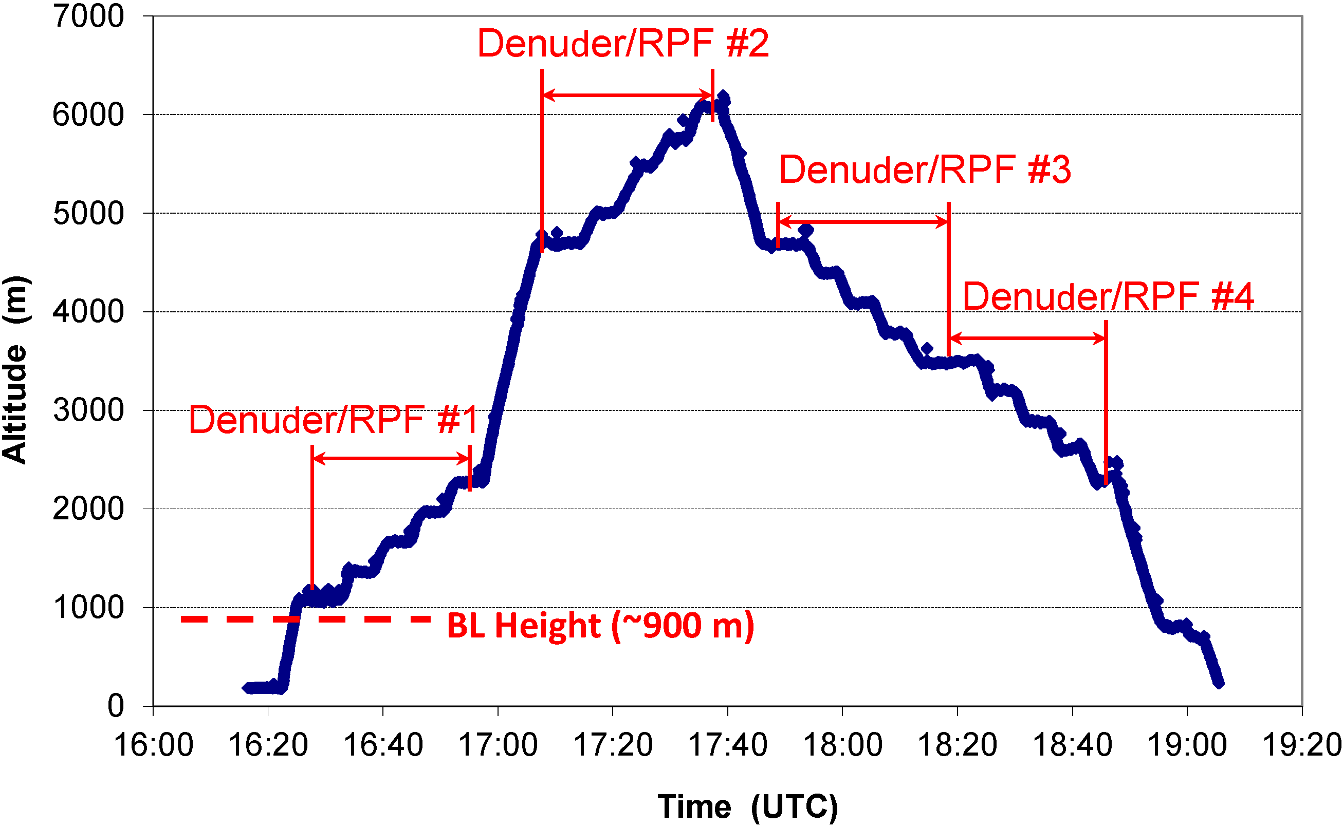
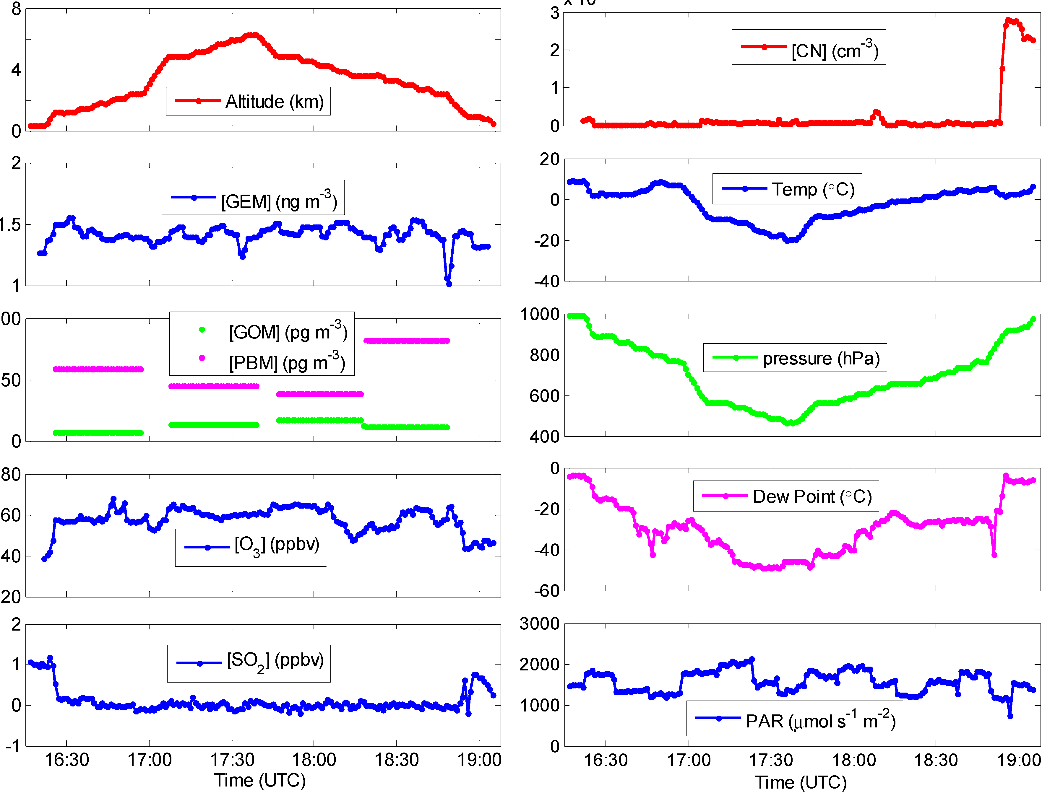
2.1. A Typical Flight
2.2. Overall Hg Speciation


| Species | Sample # | Max (pg∙m−3) | Min (pg∙m−3) | Mean ± SD (pg∙m−3) | Median (pg∙m−3) |
|---|---|---|---|---|---|
| GEM_air * | 1813 | 2050 | 750 | 1380 ± 174 | 1400 |
| GOM_air * | 106 | 125.6 | 3.1 | 34.3 ± 28.9 | 22.5 |
| PBM_air * | 53 | 194.9 | 4.4 | 29.6 ± 29.5 | 25.3 |
| GEM_gnd ** | 26 | 1610 | 1170 | 1350 ± 109 | 1320 |
| GOM_gnd ** | 27 | 12.3 | 0.6 | 2.3±2.4 | 1.80 |
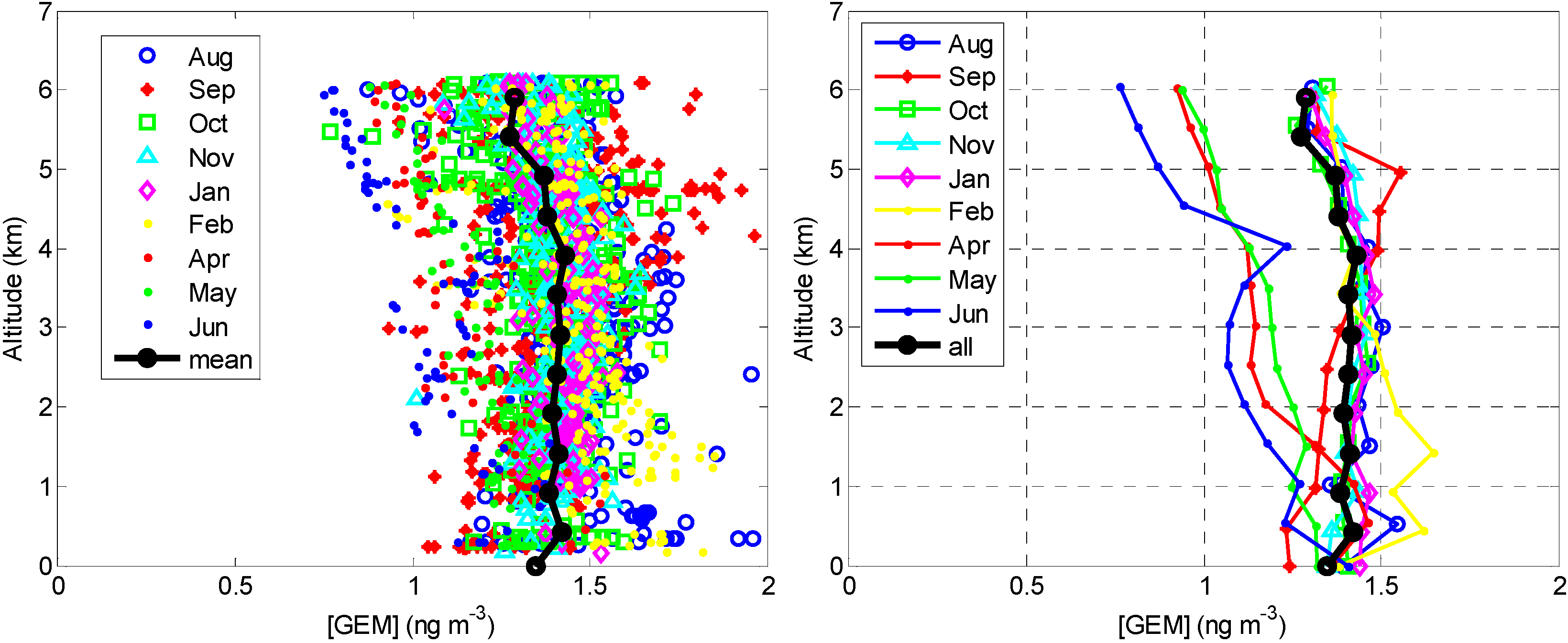
2.2.1. GEM

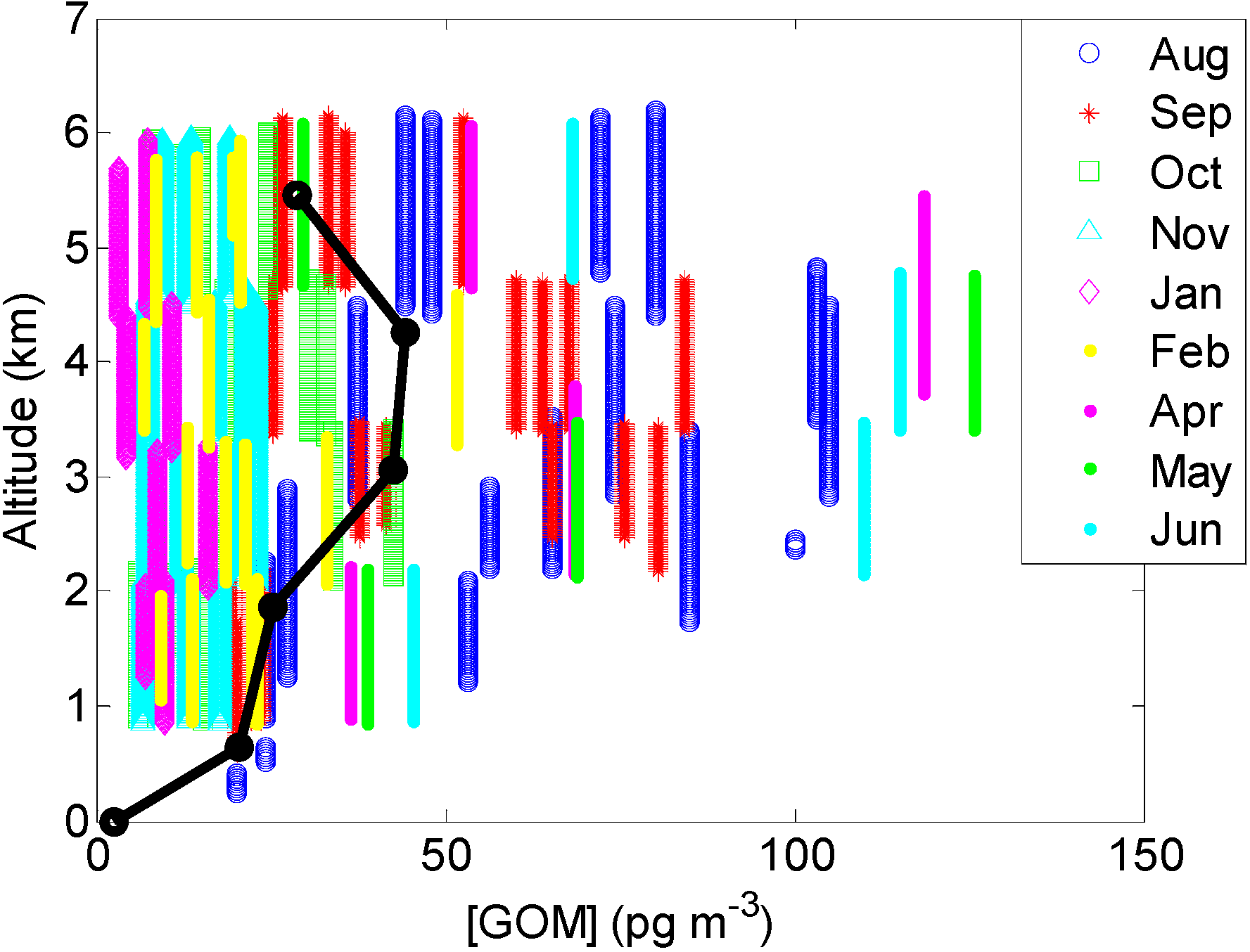
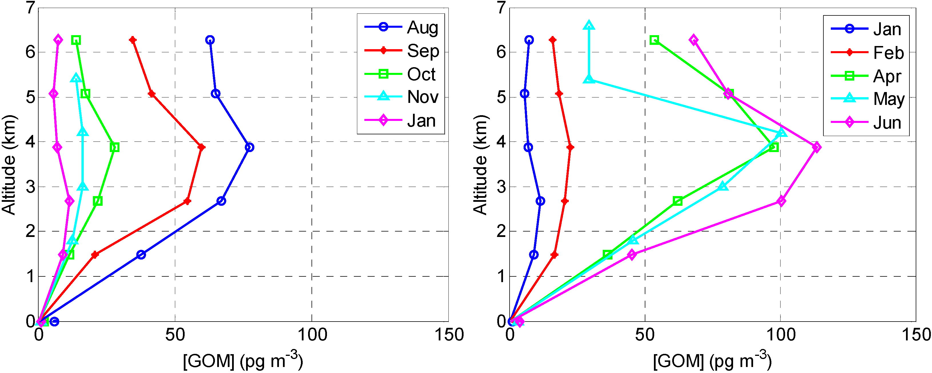
2.2.2. GOM


2.2.3. PBM

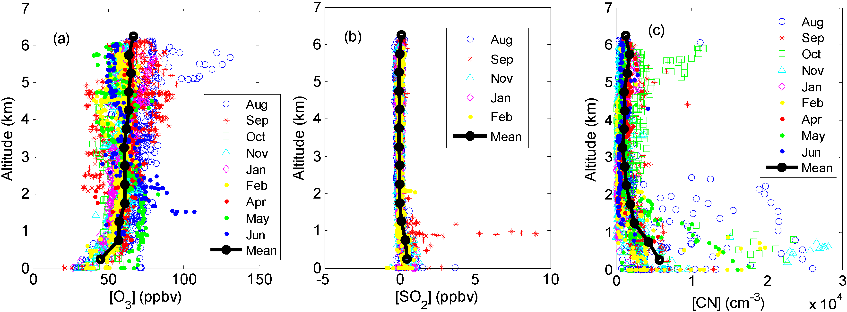
2.3. Other Supporting Measurements

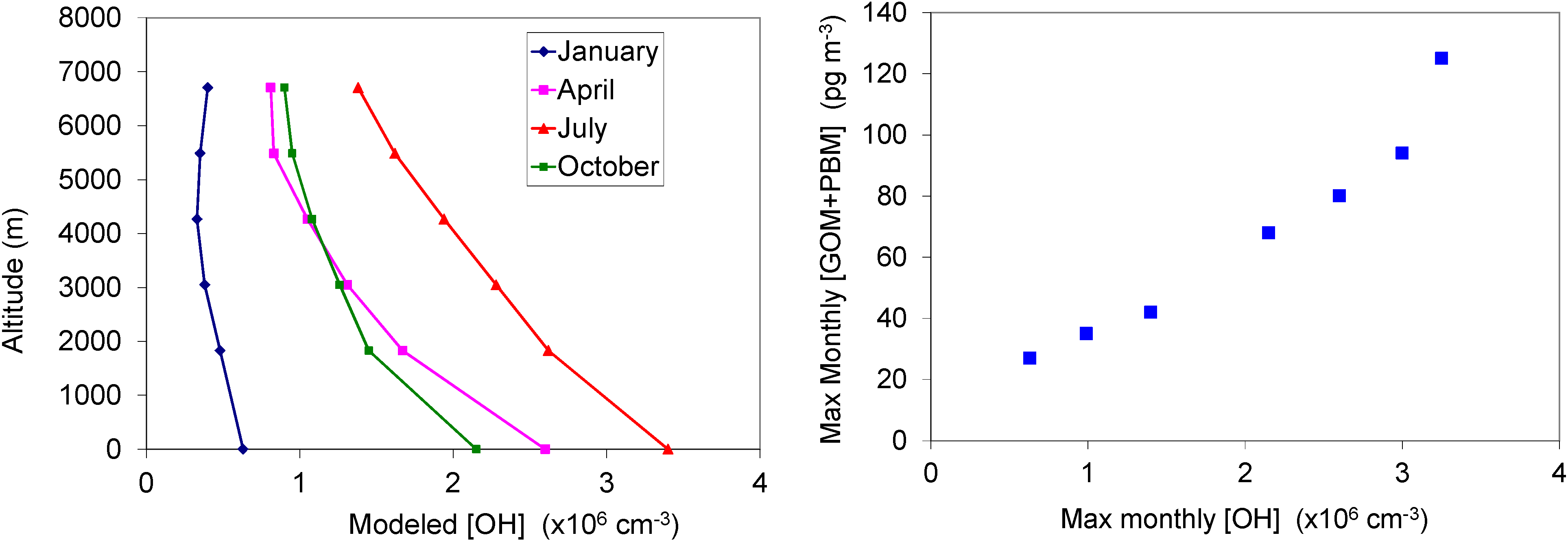
2.4. Oxidation of GEM via Hydroxyl Radical

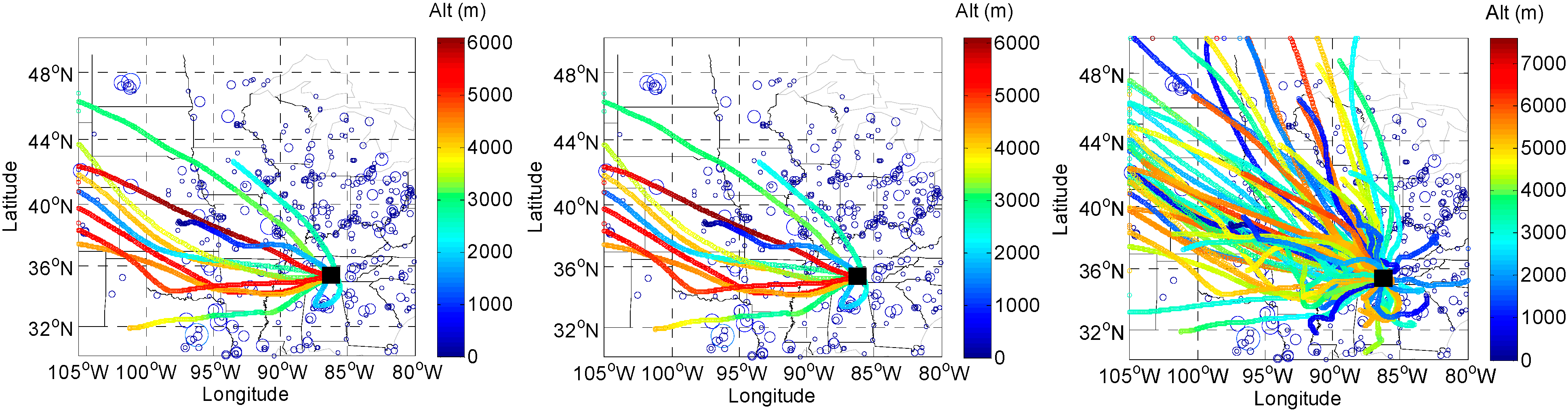
2.5. HYSPLIT back Trajectory Analysis

3. Experimental Section
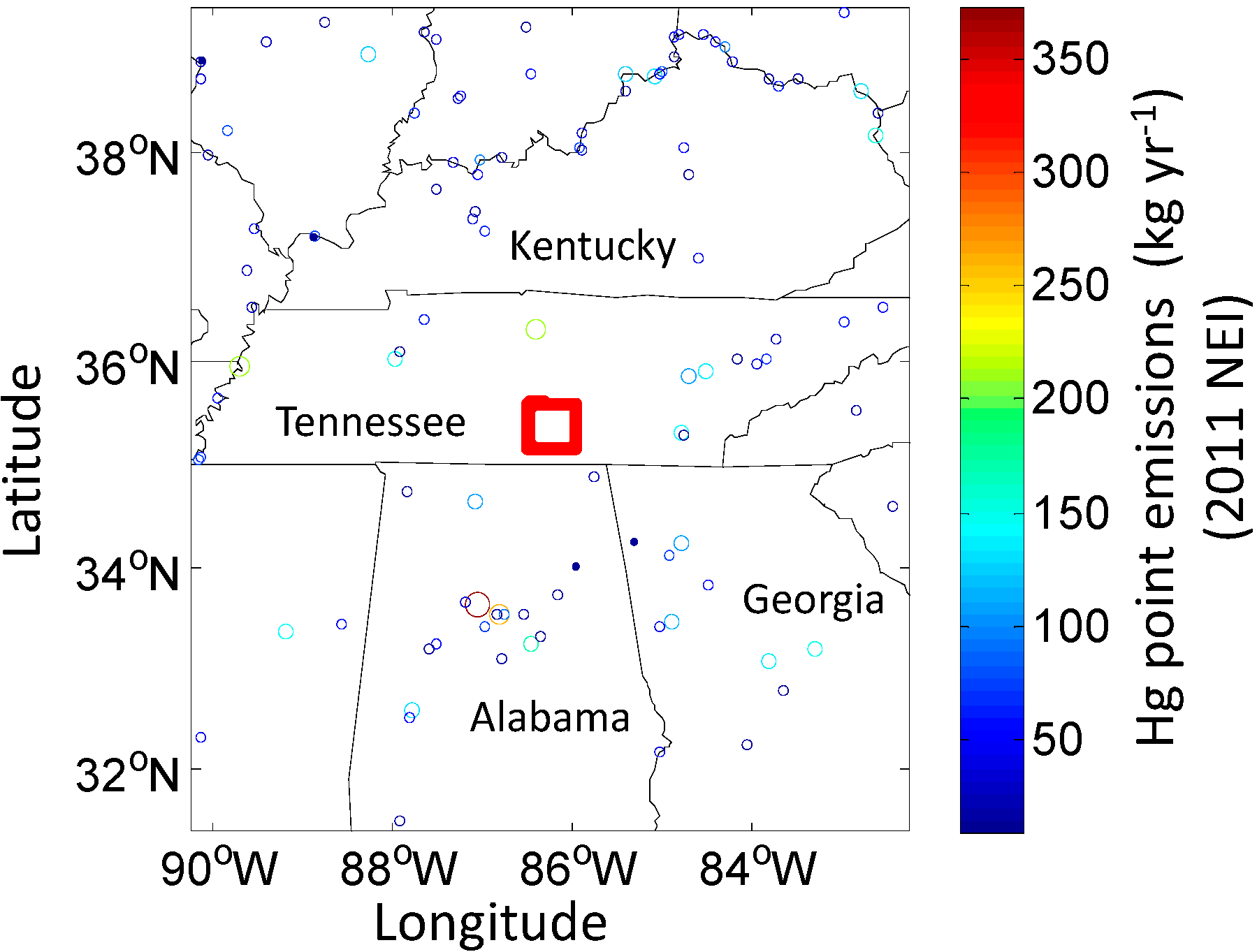
3.1. Study Area

3.2. Measurements
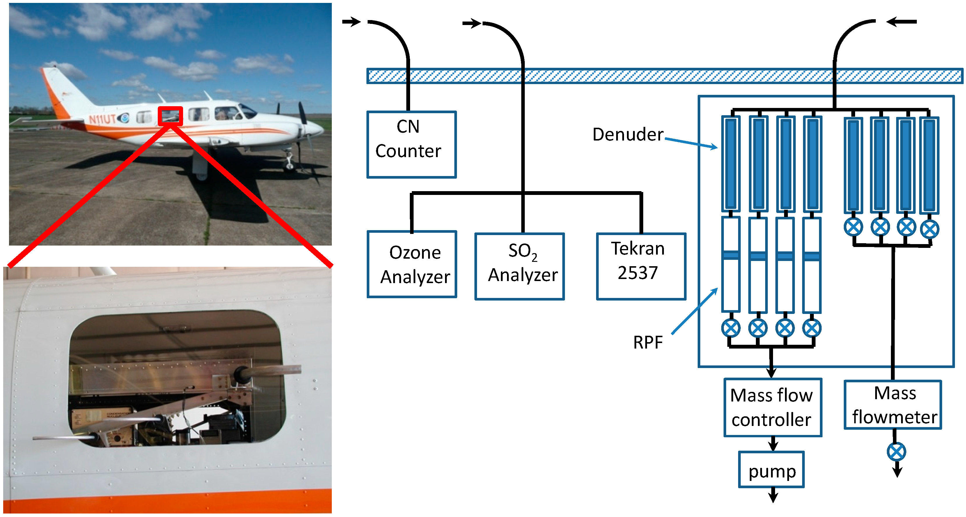
3.2.1. Aircraft Measurements

| Month | # of Flights | Dates |
|---|---|---|
| August, 2012 | 5 | 3,6,7,8 and 9 August |
| September, 2012 | 5 | 10,11,12,13 and 14 September |
| October, 2012 | 5 | 15,16,17,18 (day), 18 (night) October |
| November, 2012 | 4 | 13,14, 15 and 16 November |
| January, 2013 | 2 | 18 and 31 January |
| February, 2013 | 4 | 1,4,5 and 6 February |
| April, 2013 | 1 | 10 April |
| May, 2013 | 1 | 14 May |
| June, 2013 | 1 | 4 June |
| Total | 28 Flights |
3.2.2. Ground-Based Measurements
3.3. HYSPLIT Trajectory Model
4. Conclusions
Acknowledgments
Author Contributions
Conflicts of Interest
References
- Swartzendruber, P.C.; Jaffe, D.A.; Finley, B. Development and first results of an aircraft-based, high time resolution technique for gaseous elemental and reactive (oxidized) gaseous mercury. Environ. Sci. Technol. 2009, 43, 7484–7489. [Google Scholar] [CrossRef]
- Murphy, D.M.; Hudson, P.K.; Thomson, D.S.; Sheridan, P.J.; Wilson, J.C. Observations of mercury-containing aerosols. Environ. Sci. Technol. 2006, 40, 3163–3167. [Google Scholar] [CrossRef]
- Lyman, S.N.; Jaffe, D.A. Formation and fate of oxidized mercury in the upper troposphere and lower stratosphere. Nat. Geosci. 2012, 5, 114–117. [Google Scholar] [CrossRef]
- Fain, X.; Obrist, D.; Hallar, A.G.; Mccubbin, I.; Rahn, T. High levels of reactive gaseous mercury observed at a high elevation research laboratory in the Rocky Mountains. Atmos. Chem. Phys. 2009, 9, 8049–8060. [Google Scholar]
- Swartzendruber, P.C.; Jaffe, D.A.; Prestbo, E.M.; Weiss-Penzias, P.; Selin, N.E.; Park, R.; Jacob, D.J.; Strode, S.; Jaegle, L. Observations of reactive gaseous mercury in the free troposphere at the Mount Bachelor Observatory. J. Geophys. Res.: Atmos. 2006. [Google Scholar] [CrossRef]
- Gay, D.A.; Schmeltz, D.; Prestbo, E.; Olson, M.; Sharac, T.; Tordon, R. The atmospheric mercury network: Measurement and initial examination of an ongoing atmospheric mercury record across North America. Atmos. Chem. Phys. 2013, 13, 11339–11349. [Google Scholar]
- Bullock, O.R.; Atkinson, D.; Braverman, T.; Civerolo, K.; Dastoor, A.; Davignon, D.; Ku, J.Y.; Lohman, K.; Myers, T.C.; Park, R.J.; et al. The North American Mercury Model Intercomparison Study (NAMMIS): Study description and model-to-model comparisons. J. Geophys. Res.: Atmos. 2008. [Google Scholar] [CrossRef]
- Seigneur, C.; Karamchandani, P.; Lohman, K.; Vijayaraghavan, K.; Shia, R.L. Multiscale modeling of the atmospheric fate and transport of mercury. J. Geophys. Res.: Atmos. 2001, 106, 27795–27809. [Google Scholar] [CrossRef]
- Selin, N.E.; Jacob, D.J.; Yantosca, R.M.; Strode, S.; Jaegle, L.; Sunderland, E.M. Global 3-D land-ocean-atmosphere model for mercury: Present-day versus preindustrial cycles and anthropogenic enrichment factors for deposition. Glob. Biogeochem. Cycles 2008. [Google Scholar] [CrossRef]
- Dastoor, A.P.; Larocque, Y. Global circulation of atmospheric mercury: A modelling study. Atmos. Environ. 2004, 38, 147–161. [Google Scholar] [CrossRef]
- Holmes, C.D.; Jacob, D.J.; Corbitt, E.S.; Mao, J.; Yang, X.; Talbot, R.; Slemr, F. Global atmospheric model for mercury including oxidation by bromine atoms. Atmos. Chem. Phys. 2010, 10, 12037–12057. [Google Scholar]
- Nair, U.S.; Wu, Y.; Justin, W.; Jansen, J.; Edgerton, E.S. Diurnal and seasonal variation of mercury species at coastal-suburban, urban, and rural sites in the southeastern United States. Atmos. Environ. 2012, 47, 499–508. [Google Scholar] [CrossRef]
- Holmes, C.D.; Jacob, D.J.; Yang, X. Global lifetime of elemental mercury against oxidation by atomic bromine in the free troposphere. Geophys. Res. Lett. 2006. [Google Scholar] [CrossRef]
- Lin, C.J.; Pongprueksa, P.; Lindberg, S.E.; Pehkonen, S.O.; Byun, D.; Jang, C. Scientific uncertainties in atmospheric mercury models I: Model science evaluation. Atmos. Environ. 2006, 40, 2911–2928. [Google Scholar]
- Sommar, J.; Gardfeldt, K.; Stromberg, D.; Feng, X.B. A kinetic study of the gas-phase reaction between the hydroxyl radical and atomic mercury. Atmos. Environ. 2001, 35, 3049–3054. [Google Scholar] [CrossRef]
- Pal, B.; Ariya, P.A. Gas-phase HO center dot-Initiated reactions of elemental mercury: Kinetics, product studies, and atmospheric implications. Environ. Sci. Technol. 2004, 38, 5555–5566. [Google Scholar] [CrossRef]
- Tossell, J.A. Calculation of the energetics for oxidation of gas-phase elemental Hg by Br and BrO. J. Phys. Chem. A 2003, 107, 7804–7808. [Google Scholar]
- Goodsite, M.E.; Plane, J.M.C.; Skov, H. A theoretical study of the oxidation of Hg0 to HgBr2 in the troposphere. Environ. Sci. Technol. 2004, 38, 1772–1776. [Google Scholar] [CrossRef]
- Goodsite, M.E.; Plane, J.M.C.; Skov, H. Correction to a theoretical study of the oxidation of Hg0 to HgBr2 in the troposphere. Environ. Sci. Technol. 2012, 46, 5262–5262. [Google Scholar] [CrossRef]
- Calvert, J.G.; Lindberg, S.E. Mechanisms of mercury removal by O-3 and OH in the atmosphere. Atmos. Environ. 2005, 39, 3355–3367. [Google Scholar] [CrossRef]
- Hynes, A.J.; Donohoue, D.L.; Goodsite, M.E.; Hedgecock, I.M. Our current understanding of major chemical and physical processes affecting mercury dynamics in the atmosphere and at the air-water/terrestrial interfaces. In Mercury Fate and Transport in the Global Atmosphere: Emissions, Measurements and Models; Pirrone, N., Mason, R.P., Eds.; Springer: Berlin, Germany, 2009; pp. 427–457. [Google Scholar]
- Seigneur, C.; Lohman, K. Effect of bromine chemistry on the atmospheric mercury cycle. J. Geophys. Res.: Atmos. 2008. [Google Scholar] [CrossRef]
- Dastoor, A.P.; Davignon, D.; Theys, N.; Van Roozendael, M.; Steffen, A.; Ariya, P.A. Modeling dynamic exchange of gaseous elemental mercury at polar sunrise. Environ. Sci. Technol. 2008, 42, 5183–5188. [Google Scholar] [CrossRef]
- Fishman, J.; Crutzen, P. The Distribution of the Hydroxyl Radical in the Troposphere; Department of Atmospheric Science. Colorado State University: Fort Collins, CO, USA, 1978. [Google Scholar]
- Berresheim, H.; Plass-Dulmer, C.; Elste, T.; Mihalopoulos, N.; Rohrer, F. OH in the coastal boundary layer of Crete during MINOS: Measurements and relationship with ozone photolysis. Atmos. Chem. Phys. 2003, 3, 639–649. [Google Scholar]
- Luke, W.T.; Arnold, J.R.; Watson, T.B.; Dasgupta, P.K.; Li, J.Z.; Kronmiller, K.; Hartsell, B.E.; Tamanini, T.; Lopez, C.; King, C. The NOAA Twin Otter and its role in BRACE: A comparison of aircraft and surface trace gas measurements. Atmos. Environ. 2007, 41, 4190–4209. [Google Scholar] [CrossRef]
- Luke, W.T.; Kelley, P.; Lefer, B.L.; Flynn, J.; Rappengluck, B.; Leuchner, M.; Dibb, J.E.; Ziemba, L.D.; Anderson, C.H.; Buhr, M. Measurements of primary trace gases and NOy composition in Houston, Texas. Atmos. Environ. 2010, 44, 4068–4080. [Google Scholar] [CrossRef]
- Luke, W.T. Evaluation of a commercial pulsed fluorescence detector for the measurement of low-level SO2 concentrations during the gas-phase sulfur intercomparison experiment. J. Geophys. Res.: Atmos. 1997, 102, 16255–16265. [Google Scholar] [CrossRef]
- Lyman, S.N.; Jaffe, D.A.; Gustin, M.S. Release of mercury halides from KCl denuders in the presence of ozone. Atmos. Chem. Phys. 2010, 10, 8197–8204. [Google Scholar] [Green Version]
- Gustin, M.S.; Huang, J.Y.; Miller, M.B.; Peterson, C.; Jaffe, D.A.; Ambrose, J.; Finley, B.D.; Lyman, S.N.; Call, K.; Talbot, R.; et al. Do we understand what the mercury speciation instruments are actually measuring? Results of RAMIX. Environ. Sci. Technol. 2013, 47, 7295–7306. [Google Scholar]
- Ren, X.; Luke, W.T.; Kelley, P.; Cohen, M.; Ngan, F.; Artz, R.; Walker, J.; Brooks, S.; Moore, C.; Swartzendruber, P.; et al. Mercury speciation at a coastal site in the northern Gulf of Mexico: Results from the Grand Bay intensive studies in summer 2010 and spring 2011. Atmosphere 2014, 5, 230–251. [Google Scholar] [CrossRef]
- Draxler, R.R.; Rolph, G.D. HYSPLIT (HYbrid Single-Particle Lagrangian Integrated Trajectory) Model; NOAA Air Resources Laboratory: College Park, MD, USA, 2014. [Google Scholar]
- Steffen, A.; Scherz, T.; Olson, M.; Gay, D.; Blanchard, P. A comparison of data quality control protocols for atmospheric mercury speciation measurements. J. Environ. Monit. 2012, 14, 752–765. [Google Scholar] [CrossRef]
© 2014 by the authors; licensee MDPI, Basel, Switzerland. This article is an open access article distributed under the terms and conditions of the Creative Commons Attribution license (http://creativecommons.org/licenses/by/3.0/).
Share and Cite
Brooks, S.; Ren, X.; Cohen, M.; Luke, W.T.; Kelley, P.; Artz, R.; Hynes, A.; Landing, W.; Martos, B. Airborne Vertical Profiling of Mercury Speciation near Tullahoma, TN, USA. Atmosphere 2014, 5, 557-574. https://doi.org/10.3390/atmos5030557
Brooks S, Ren X, Cohen M, Luke WT, Kelley P, Artz R, Hynes A, Landing W, Martos B. Airborne Vertical Profiling of Mercury Speciation near Tullahoma, TN, USA. Atmosphere. 2014; 5(3):557-574. https://doi.org/10.3390/atmos5030557
Chicago/Turabian StyleBrooks, Steve, Xinrong Ren, Mark Cohen, Winston T. Luke, Paul Kelley, Richard Artz, Anthony Hynes, William Landing, and Borja Martos. 2014. "Airborne Vertical Profiling of Mercury Speciation near Tullahoma, TN, USA" Atmosphere 5, no. 3: 557-574. https://doi.org/10.3390/atmos5030557