
New Laboratory Experiments to Study the Large-Scale Circulation and Climate Dynamics
 , , , , , , and
Abstract
:1. Introduction
2. Experimental Setup
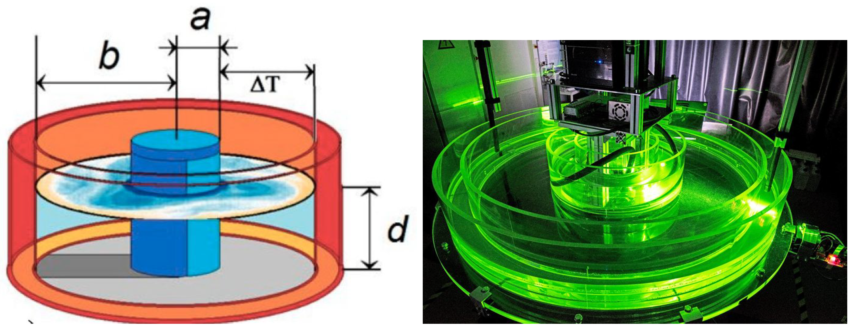
2.1. The BTU Experiment

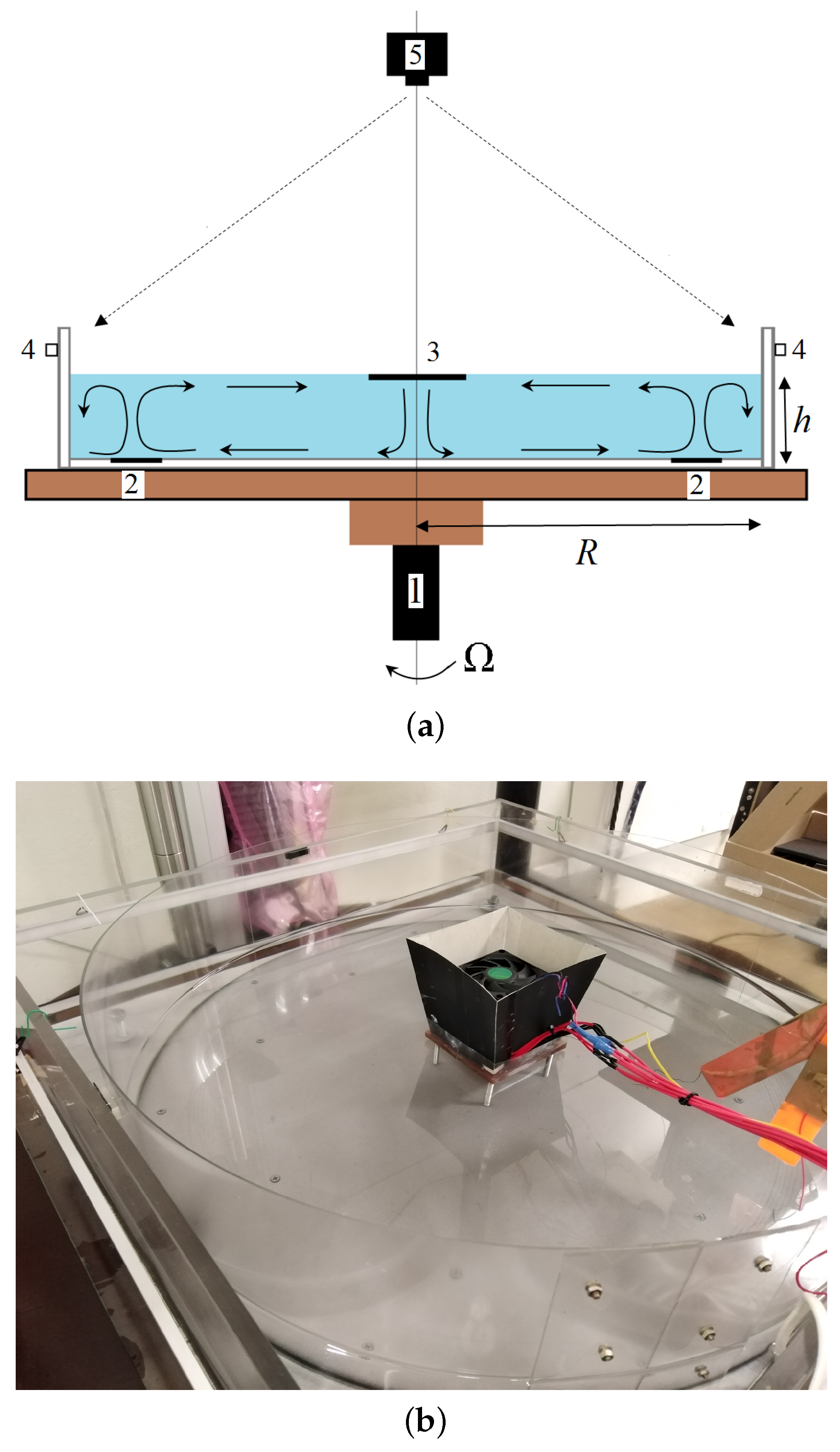
2.2. The ICMM Experiment
2.3. Specifics of the Different Experimental Models
3. Results
3.1. BTU Configuration
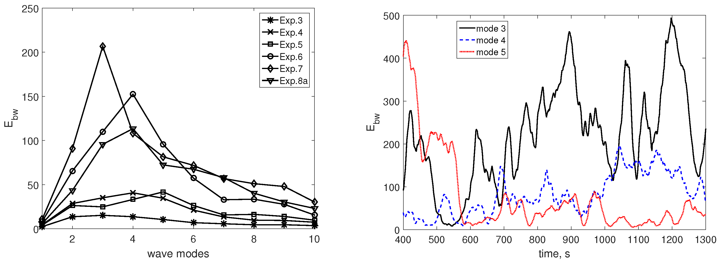
3.1.1. Spectra
3.1.2. Extreme Event Distributions
3.1.3. Local Instabilities as Rare Events
3.2. Numerical Simulation
3.3. The ICMM Configuration
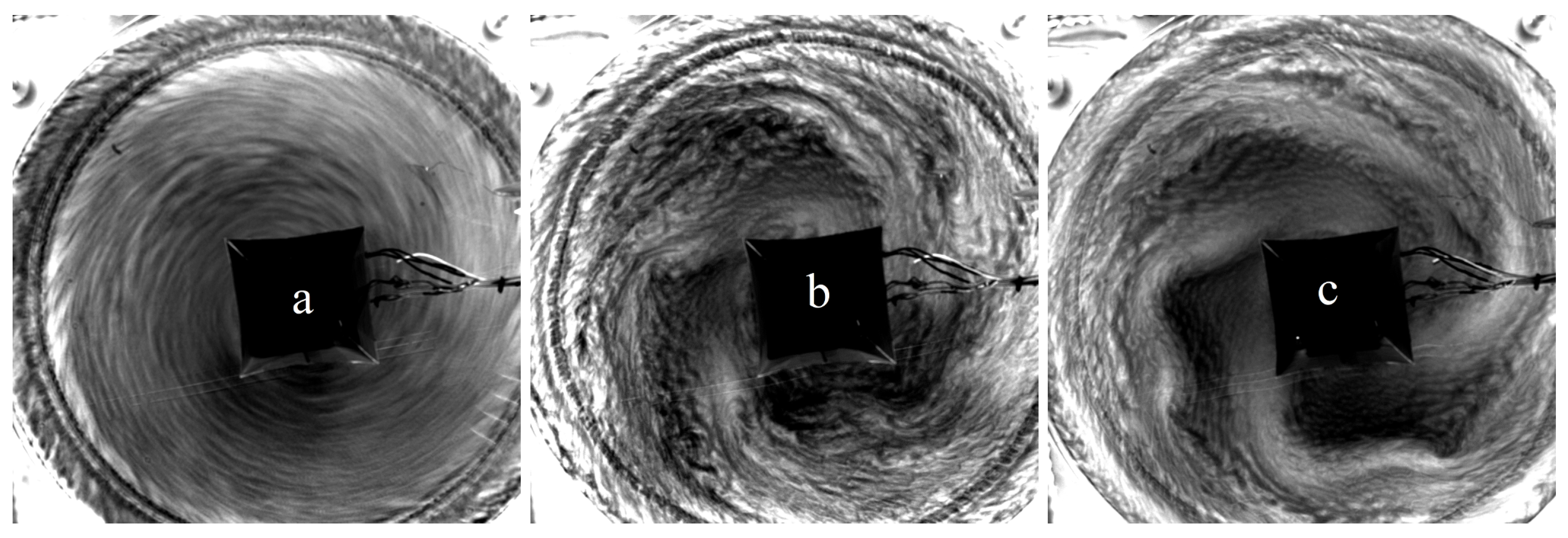
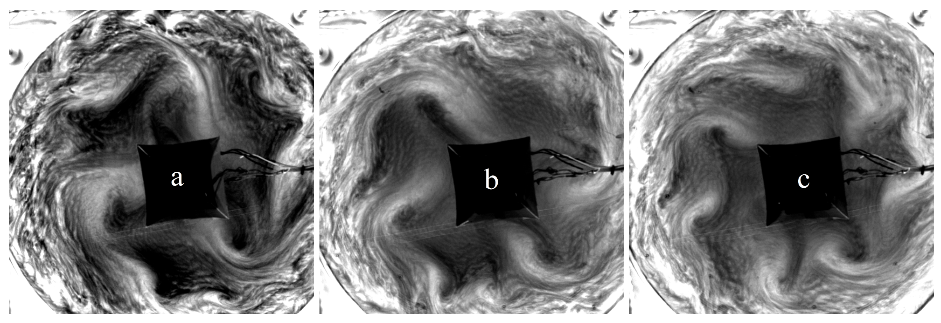
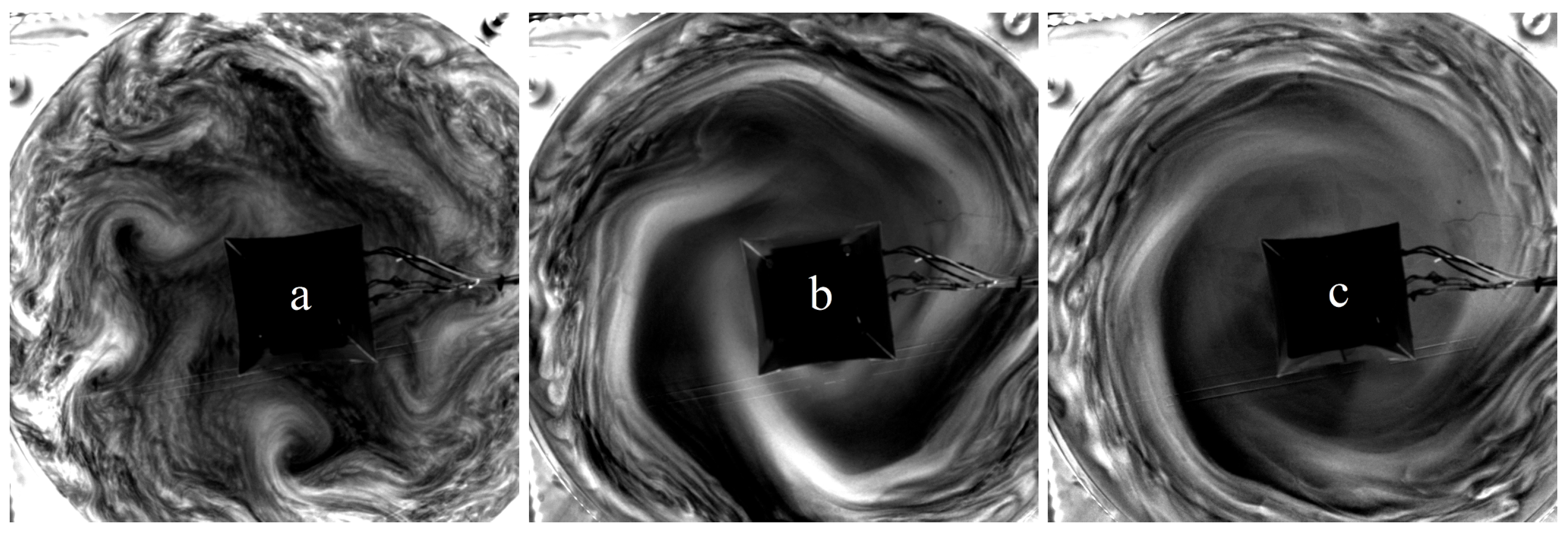
3.3.1. Experiment
3.3.2. Numerical Simulation
4. Discussion
5. Conclusions
Author Contributions
Funding
Institutional Review Board Statement
Informed Consent Statement
Data Availability Statement
Acknowledgments
Conflicts of Interest
References
- Vallis, G.K. Atmospheric and Oceanic Fluid Dynamics: Fundamentals and Large-Scale Circulation, 2nd ed.; Cambridge University Press: Cambridge, UK, 2017. [Google Scholar] [CrossRef]
- Rossby, C.G. On the solution of problems of atmospheric motion by means of model experiments. Mon. Weather Rev. 1926, 54, 237–241. [Google Scholar] [CrossRef]
- Hughes, G.O.; Griffiths, R.W. Horizontal convection. Annu. Rev. Fluid Mech. 2008, 40, 185–208. [Google Scholar] [CrossRef]
- Passaggia, P.Y.; Hurley, M.W.; White, B.; Scotti, A. Turbulent horizontal convection at high Schmidt numbers. Rev. Phys. Fluids 2017, 2, 090506. [Google Scholar] [CrossRef]
- Baker, D.J.; Robinson, A.R. A laboratory model for the general ocean circulation. Philos. Trans. R. Soc. 1969, 265, 533–566. [Google Scholar]
- McEwan, A.D. Angular momentum diffusion and the initiation of cyclones. Nature 1976, 260, 126–128. [Google Scholar] [CrossRef]
- Sukhanovskii, A.; Popova, E. The importance of horizontal rolls in the rapid intensification of tropical cyclones. Bound. Layer Meteorol. 2020, 175, 259–276. [Google Scholar] [CrossRef]
- Fultz, D.; Long, R.R.; Owens, G.V.; Weil, J. Two-dimensional flow around a circular barrier in a rotating shell. AMS Meteorol. Monogr. 1959, 4, 21. [Google Scholar]
- Hide, R.; Mason, P.J. Sloping convection in a rotating fluid. Adv. Phys. 1975, 24, 47–100. [Google Scholar] [CrossRef]
- Read, P.L. Chapter 4.3—Rotating annulus flows and baroclinic waves. In Rotating Fluids in Geophysical and Industrial Applications; Hopfinger, E.J., Ed.; Springer: Wien, Austria, 1992; pp. 185–216. [Google Scholar]
- Read, P.L.; Perez, E.P.; Moraz, I.M.; Young, R.M.B. Chapter 1—Circulation of planetary atmospheres: Insights from rotating annulus and related experiments. In Modeling Atmospheric and Oceanic Flows: Insight from Laboratory Experiments and Numerical Simulations; von Larcher, T., Williams, P.D., Eds.; Wiley: Hoboken, NJ, USA, 2014; pp. 9–45. [Google Scholar]
- Hide, R. A path of discovery in geo physical fluid dynamics. Astron. Geophys. 2010, 51, 4.16–4.23. [Google Scholar] [CrossRef]
- Ghil, M.; Read, P.L.; Smith, L. Geophysical flows as dynamical systems: The influence of Hide’s experiments. Astron. Geophys. 2010, 51, 4.28–4.35. [Google Scholar] [CrossRef]
- Exner, F.M. Über die Bildung von Windhosen und Zyklonen. Sitzungsberichte der Akademie der Wiss. Wien, Abt. Ha 1923, 132, 1–16. [Google Scholar]
- Fultz, D. Experimental analogies to atmospheric motions. In Compendium of Meteorology; Malone, T.F., Ed.; American Meteorological Society: Boulder, CO, USA, 1951. [Google Scholar]
- Osman, M.B.; Coats, S.; Das, S.B.; Chellman, N. North Atlantic jet stream projections in the context of the past 1250 years. PNAS 2021, 118, e2104105118. [Google Scholar] [CrossRef] [PubMed]
- Stendel, M.; Francis, J.; White, R.; Williams, P.D.; Woollings, T. Chapter 15—The jet stream and climate change. In Climate Change (Third Edition); Letcher, T.M., Ed.; Elsevier: Amsterdam, The Netherlands, 2021; pp. 327–357. [Google Scholar] [CrossRef]
- Alizadeh, O.; Lin, Z. Rapid Arctic warming and its link to the waviness and strength of the westerly jet stream over West Asia. Glob. Planet. Chang. 2021, 199, 103447. [Google Scholar] [CrossRef]
- Francis, J.A.; Vavrus, S.J. Evidence for a wavier jet stream in response to rapid Arctic warming. Environ. Res. Lett. 2015, 10, 014005. [Google Scholar] [CrossRef]
- Rodda, C.; Harlander, U.; Vincze, M. Jet stream variability in a polar warming scenario–a laboratory perspective. Weather Clim. Dynam. 2022, 3, 937–950. [Google Scholar] [CrossRef]
- Moon, W.; Kim, B.M.; Yang, G.H.; Wettlaufer, J.S. Wavier jet streams driven by zonally asymmetric surface thermal forcing. Proc. Natl. Acad. Sci. USA 2022, 119, e2200890119. [Google Scholar] [CrossRef] [PubMed]
- Borchert, S.; Achatz, U.; Fruman, M.D. Gravity wave emission in an atmosphere-like configuration of the differentially heated rotating annulus experiment. J. Fluid Mech. 2014, 758, 287–311. [Google Scholar] [CrossRef]
- Rodda, C.; Hien, S.; Achatz, U.; Harlander, U. A new atmospheric-like differentially heated rotating annulus configuration to study gravity wave emission from jets and fronts. Exp. Fluids 2019, 62, 2. [Google Scholar] [CrossRef]
- Scolan, H.; Read, P.L. A rotating annulus driven by localized convective forcing: A new atmosphere-like experiment. Exp. Fluids 2017, 58, 75. [Google Scholar] [CrossRef]
- Sukhanovskii, A.; Popova, E. A shallow layer laboratory model of large-scale atmospheric circulation. arXiv 2022, arXiv:2210.15266. [Google Scholar]
- Banerjee, A.K.; Bhattacharyaa, A.; Balasubramaniana, S. Experimental study of rotating convection in the presence of bi-directional thermal gradients with localized heating. AIP Adv. 2018, 8, 115324. [Google Scholar] [CrossRef]
- Vincze, M.; Borcia, I.D.; Harlander, U. Temperature fluctuations in a changing climate: An ensemble based experimental approach. Sci. Rep. 2017, 7, 254. [Google Scholar] [CrossRef] [PubMed]
- Vincze, M.; Bozóki, T.; Herein, M.; Borcia, I.D.; Harlander, U.; Horicsányi, A.; Nyerges, A.; Rodda, C.; Pál, A.; Pálfy, J. The Drake Passage opening from an experimental fluid dynamics point of view. Sci. Rep. 2021, 11, 19951. [Google Scholar] [CrossRef] [PubMed]
- Rodda, C.; Harlander, U. Transition from geostrophic flows to inertia-gravity waves in the spectrum of a differentially heated rotating annulus experiment. J. Atmos. Sci. 2020, 77, 2793–2806. [Google Scholar] [CrossRef]
- Read, P.L. Dynamics and circulation regimes of terrestrial planets. Planet. Space Sci. 2011, 59, 900–914. [Google Scholar] [CrossRef]
- Folis, W.W.; Hide, R. Thermal convection in a rotating annulus of liquid: Effect of viscosity on the transition between axisymmetric and non-axisymmetric flow regimes. J. Atmos. Sci. 1965, 22, 541–558. [Google Scholar]
- Rodda, C. Gravity Wave Emission from Jet Systems in the Differentially Heated Rotating Annulus Experiment; Cuvillier Verlag: Göttingen, Germany, 2019; p. 200. [Google Scholar]
- Fultz, D.; Long, R.R.; Owens, G.V.; Bohan, W.; Kaylor, R.; Weil, J. Studies of Thermal Convection in a Rotating Cylinder with Some Implications for Large-Scale Atmospheric Motions; American Met. Soc.: Boston, MA, USA, 1959; pp. 1–104. [Google Scholar] [CrossRef]
- Fein, J.S.; Pfeffer, R.L. An experimental study of the effects of Prandtl number on thermal convection in a rotating, differentially heated cylindrical annulus of fluid. J. Fluid Mech. 1976, 75, 81–112. [Google Scholar] [CrossRef]
- Manikantan, H.; Squires, T.M. Surfactant dynamics: Hidden variables controlling fluid flows. J. Fluid Mech. 2020, 892, 1. [Google Scholar] [CrossRef]
- Harlander, U.; Borcia, I.D.; Vincze, M.; Rodda, C. Probability Distribution of Extreme Events in a Baroclinic Wave Laboratory Experiment. Fluids 2022, 7, 274. [Google Scholar] [CrossRef]
- Nastrom, G.D.; Gage, K.S. A Climatology of Atmospheric Wavenumber Spectra of Wind and Temperature Observed by Commercial Aircraft. J. Atmos. Sci. 1985, 42, 950–960. [Google Scholar] [CrossRef]
- Lindborg, E. A Helmholtz decomposition of structure functions and spectra calculated from aircraft data. J. Fluid Mech. 2015, 762, R4. [Google Scholar] [CrossRef]
- Terasaki, K.; Tanaka, H.L.; Žagar, N. Energy spectra of Rossby and gravity waves. SOLA 2011, 7, 45–48. [Google Scholar] [CrossRef]
- Callies, J.; Ferrari, R.; Bühler, O. Transition from geostrophic turbulence to inertia–gravity waves in the atmospheric energy spectrum. Proc. Natl. Acad. Sci. USA 2014, 111, 17033–17038. [Google Scholar] [CrossRef]
- de Bruyn Kops, S.M.; Riley, J.J.; Winters, K.B. Chapter 2—Reynolds and Froude number scaling in stably-stratified flow. In IUTAM Symposium on Reynolds Number Scaling in Turbulent Flow; Smits, A.J., Ed.; Springer Science + Business Media: Dordrecht, The Netherlands, 2004; pp. 71–76. [Google Scholar]
- Vincze, M.; Borchert, S.; Achatz, U.; von Larcher, T.; Baumann, M.; Liersch, C.; Remmler, S.; Beck, T.; Alexandrov, K.D.; Egbers, C.; et al. Benchmarking in a rotating annulus: A comparative experimental and numerical study of baroclinic wave dynamics. Meteorol. Z. 2015, 23, 611–635. [Google Scholar] [CrossRef]
- Wright, S.; Su, S.; Scolan, H.; Young, R.M.B.; Read, P.L. Regimes of Axisymmetric Flow and Scaling Laws in a Rotating Annulus with Local Convective Forcing. Fluids 2017, 2, 41. [Google Scholar] [CrossRef]
- Abide, S.; Viazzo, S.; Raspo, I.; Randriamampianina, A. Higher-order compact scheme for high-performance computing of stratified rotating flows. Comput. Fluids 2018, 174, 300–310. [Google Scholar] [CrossRef]
- Meletti, G.; Abide, S.; Viazzo, S.; Harlander, U. A parameter study of strato-rotational low-frequency modulations: Impacts on momentum transfer and energy distribution. In Taylor-Couette and Related Flows on the Centennial of Taylor’s Seminal Philosophical Transactions Paper (Part 2); Lueptow, R., Hollerbach, R., Serre, E., Eds.; Philosophical Transactions A: London, UK, 2023; pp. 1–22. [Google Scholar]
- Williams, G.P. Baroclinic annulus waves. J. Fluid Mech. 1971, 49, 417–449. [Google Scholar] [CrossRef]
- Vasiliev, A.; Popova, E.; Sukhanovskii, A. The flow structure in a laboratory model of general atmosphere circulation. Comput. Contin. Mech. 2023, accepted. [Google Scholar]
- Batalov, V.; Sukhanovsky, A.; Frick, P. Laboratory study of differential rotation in a convective rotating layer. Geophys. Astrophys. Fluid Dyn. 2010, 104, 349–368. [Google Scholar] [CrossRef]
- Hide, R.; Mason, P.J. Baroclinic waves in a rotating fluid subject to internal heating. Philos. Trans. R. Soc. Lond. Ser. Math. Phys. Sci. 1970, 268, 201–232. [Google Scholar] [CrossRef]
- Tajima, T.; Nakamura, T. Meridional Flow Field of Axisymmetric Flows in a Rotating Annulus. J. Atmos. Sci. 2000, 57, 3109–3121. [Google Scholar] [CrossRef]


| Geometry | BTU | ICMM | ||
|---|---|---|---|---|
| inner radius | a (mm) | 350 | - | |
| outer radius | b (mm) | 700 | 345 | |
| gap width | (mm) | 350 | 345 | |
| fluid depth | d (mm) | 60 | 30 | |
| fluid properties | ||||
| density | () | 997 | 911 | |
| kin. viscosity | () | 1.004 | 5.2 | |
| therm. diffusivity | () | 0.1434 | 0.083 | |
| exp. coefficient | (1/K) | 0.207 | 0.9 | |
| 7.0 | 62.7 |
| Heater Properties | |||
|---|---|---|---|
| BTU | |||
| thickness perspex walls | 10 | mm | |
| radius cooling chamber | 340 | mm | |
| width heating chamber | 85 | mm | |
| ICMM | |||
| heater width | l | 25 | mm |
| heater radius | 293 | mm | |
| cooler radius | 28 | mm | |
| heating power | 123 | Wt | |
| cooling power | ≈3 | Wt |
| Exp. | , rad | E | |||
|---|---|---|---|---|---|
| BTU | |||||
| 1 | 0.21 | 4 | 0.0091 | 15.2 | 0.0013 |
| 2 | 0.073 | 2.5 | 0.046 | 1.87 | 0.0038 |
| ICMM | |||||
| 1 | 0.08 | 25.1 | 8.4 | 1.7 | 0.068 |
| 2 | 0.09 | 25.7 | 6.5 | 2.3 | 0.061 |
| 3 | 0.11 | 26.9 | 4.9 | 3.2 | 0.05 |
| 4 | 0.13 | 24.5 | 3.1 | 4.7 | 0.042 |
| 5 | 0.17 | 25.1 | 1.9 | 7.5 | 0.033 |
| 6 | 0.23 | 23.9 | 1.0 | 1.4 | 0.024 |
| 7 | 0.37 | 23.9 | 0.4 | 3.6 | 0.015 |
| 8a | 0.48 | 24.5 | 0.2 | 6 | 0.012 |
| 8b | 0.48 | 10.2 | 0.1 | 6 | 0.012 |
| 8c | 0.48 | 7.2 | 0.06 | 6 | 0.012 |
| cm | |||||
|---|---|---|---|---|---|
| 5 | 4 | 3 | 2 | 1 | |
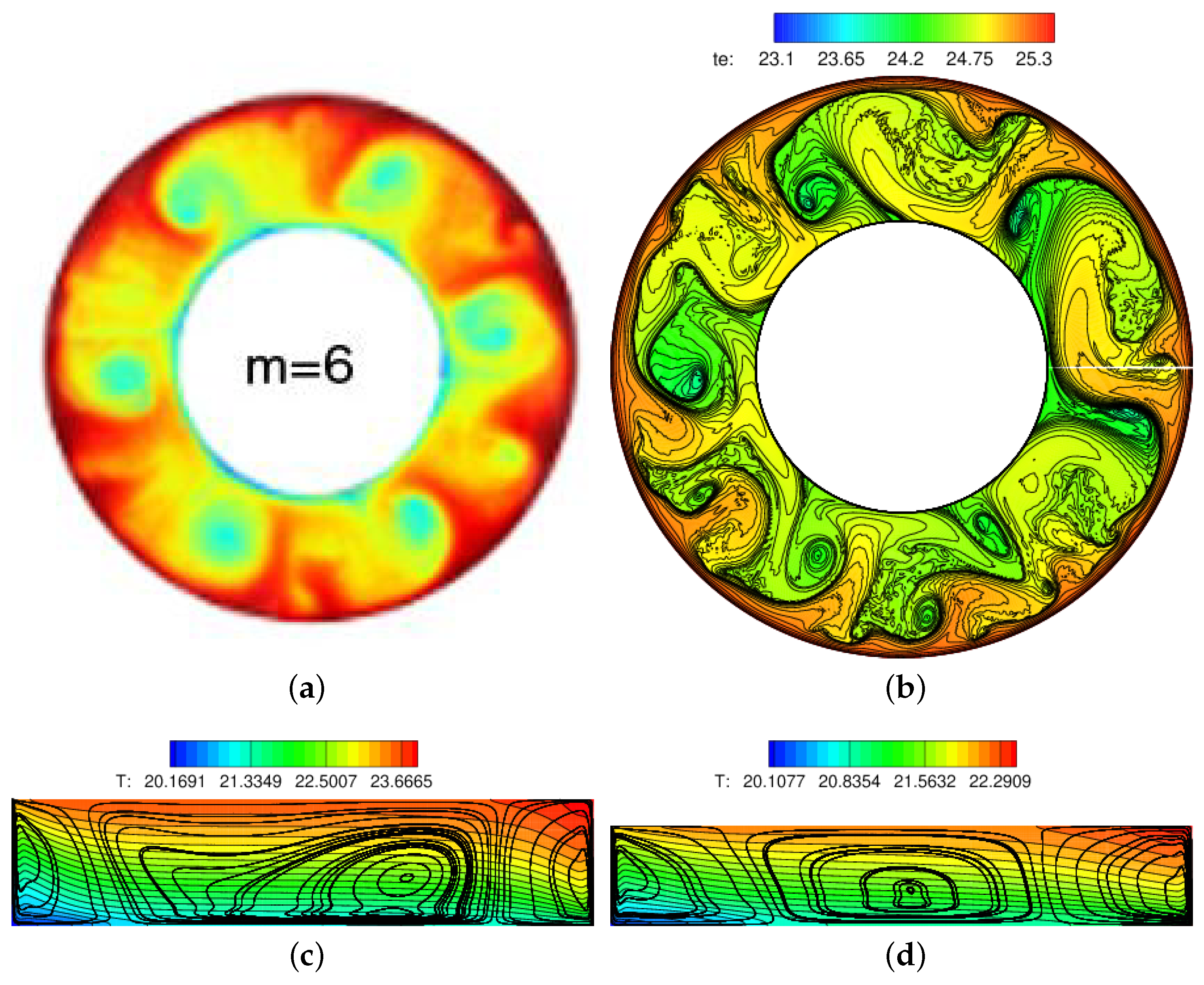
| - | - | 6 | - | - | |
| - | - | 7 | - | - | |
| - | - | 8 | - | - |
Disclaimer/Publisher’s Note: The statements, opinions and data contained in all publications are solely those of the individual author(s) and contributor(s) and not of MDPI and/or the editor(s). MDPI and/or the editor(s) disclaim responsibility for any injury to people or property resulting from any ideas, methods, instructions or products referred to in the content. |
© 2023 by the authors. Licensee MDPI, Basel, Switzerland. This article is an open access article distributed under the terms and conditions of the Creative Commons Attribution (CC BY) license (https://creativecommons.org/licenses/by/4.0/).
Share and Cite
Harlander, U.; Sukhanovskii, A.; Abide, S.; Borcia, I.D.; Popova, E.; Rodda, C.; Vasiliev, A.; Vincze, M. New Laboratory Experiments to Study the Large-Scale Circulation and Climate Dynamics. Atmosphere 2023, 14, 836. https://doi.org/10.3390/atmos14050836
Harlander U, Sukhanovskii A, Abide S, Borcia ID, Popova E, Rodda C, Vasiliev A, Vincze M. New Laboratory Experiments to Study the Large-Scale Circulation and Climate Dynamics. Atmosphere. 2023; 14(5):836. https://doi.org/10.3390/atmos14050836
Chicago/Turabian StyleHarlander, Uwe, Andrei Sukhanovskii, Stéphane Abide, Ion Dan Borcia, Elena Popova, Costanza Rodda, Andrei Vasiliev, and Miklos Vincze. 2023. "New Laboratory Experiments to Study the Large-Scale Circulation and Climate Dynamics" Atmosphere 14, no. 5: 836. https://doi.org/10.3390/atmos14050836