
Evaluation of Air–Sea Flux Parameterization for Typhoon Mangkhut Simulation during Intensification Period

1
Collaborative Innovation Center on Forecast and Evaluation of Meteorological Disasters, Key Laboratory for Aerosol-Cloud-Precipitation of China Meteorological Administration, School of Atmospheric Physics, Nanjing University of Information Science and Technology, Nanjing 210044, China
2
Southern Marine Science and Engineering Guangdong Laboratory (Zhuhai), Zhuhai 519000, China
3
State Key Laboratory of Atmospheric Boundary Layer Physics and Atmospheric Chemistry, Institute of Atmospheric Physics, Chinese Academy of Sciences, Beijing 100029, China
*
Author to whom correspondence should be addressed.
Atmosphere 2022, 13(12), 2133; https://doi.org/10.3390/atmos13122133
Submission received: 30 November 2022
/
Revised: 8 December 2022
/
Accepted: 16 December 2022
/
Published: 19 December 2022
(This article belongs to the Special Issue Atmospheric Boundary Layer Processes, Characteristics and Parameterization)
Abstract
:Using the Advanced Research Weather Research and Forecasting (WRF) model, a series of numerical experiments are conducted to examine the sensitivity of the Typhoon Mangkhut intensification simulation to different air–sea flux parameterization schemes (isftcflx option), including option 0 (OPT0), option 1 (OPT1), and option 2 (OPT2). The results show that three schemes basically reproduce tropical cyclone (TC) track and intensity of observation, and the simulated exchange coefficient of three schemes is consistent with theoretical results. Using the same upper limit of as OPT0 and OPT2, OPT1 has much larger than the other two options, which leads to larger latent heat (and sensible heat) flux and produces stronger inflow (within boundary layer) and updrafts (around eyewall), and thus stronger TC intensity. Meanwhile, the results that larger corresponds with stronger TC in the mature stage are consistent with Emanuel’s potential intensity theory. The fact that in OPT1 is evidently larger than the from previous studies leads to produce a better TC intensity simulation. Generally, we should use more reasonable air–sea flux parameterization based on observation to improve TC intensity simulation.
1. Introduction
As one of the most destructive weather systems, a tropical cyclone (TC) causes severe loss of lives and property damage around the world [1]. Over the past decades, with the development of numerical weather prediction models, TC track prediction has steadily improved, however, TC intensity forecast, especially accurate prediction of the TC intensification period, remains a challenge and problem [2].
The exchange of heat, moisture, and momentum at the air–sea interface is believed to be one of the most important physical processes determining TC intensity change [3,4,5]. The air–sea surface flux exchanges of moist enthalpy (the sum of latent and sensible heat fluxes) act as the primary energy source of TC, whereas the surface momentum flux is the sink of TC development [6]. An accurate description of the air–sea interaction processes is important to improve the forecast of TC evolution [7].
In current numerical weather prediction models, air–sea fluxes cannot be resolved directly, and therefore must be accounted for through subgrid-scale parameterizations of surface exchange coefficients [4,5]. The surface fluxes of momentum τ, sensible heat SH, and latent heat LH are expressed as
where ρ is the air density, is the specific heat capacity of air at constant pressure, is the latent heat of vaporization, is the friction velocity, and and are the surface layer temperature and moisture scales, respectively; Δ(U, θ, q) are the differences in wind speed, temperature, and water vapor between a reference height (often 10 m) and the bottom of the surface layer (U = 0), respectively. , , and are the bulk exchange coefficients for drag, sensible heat, and latent heat, respectively.
Based on the Monin–Obukhov similarity theory and observations indicating a neutrally stable surface layer within the TC eyewall (e.g., [8]), , , and in neutral stability are given as follows:
The drag coefficient , sensible heat exchange coefficient , and latent heat exchange coefficient under neutral stability conditions are calculated from
where k is the von Karman constant, is the reference height (often 10 m), the subscript n represents neutrally stable conditions, and , , and are the roughness lengths for momentum, sensible heat, and latent heat (moisture), respectively. Additionally, the enthalpy exchange coefficient is defined as the combination of the latent and sensible heat exchange [9].
Emanuel’s well-known potential intensity (PI) theory states that the potential intensity for a steady-state (or mature) TC is proportional to the ratio of surface bulk transfer coefficients for enthalpy and momentum, , and suggested the ratio in real hurricanes lies in the range 0.75–1.5 [10,11]. Clearly, the ratio is an important factor in the TC intensity of a mature storm.
Using numerical simulations, many studies have shown that TC intensity simulation is affected by the choice of air–sea flux (or surface roughness) parameterization schemes. Green and Zhang [5] examined the impact of surface flux on the intensity and structure of tropical cyclones using different air–sea flux parameterization schemes available in Weather Research and Forecasting (WRF) version 3.4 through simulations of Hurricane Katrina (2005). Chen et al. [12] focused on Hurricane Katrina (2005) through a coupled atmosphere–ocean modeling system and examined the combined impacts of air–sea flux parameterizations and ocean cooling on TC evolution. Additionally, Kueh et al. [6] investigated the effects of horizontal resolution and surface flux formulas on typhoon intensity and structure simulations through the case study of Super Typhoon Haiyan (2013). Additionally, Greeshma et al. [13] and Alimohammadi et al. [14] investigated the impact of air–sea flux parametrization schemes on the simulation of TC over the North Indian Ocean and the Arabian Sea, respectively. Furthermore, Green and Zhang [5] and Nystrom et al. [15,16] focused on the impact of surface exchange coefficient uncertainty on TC simulation through varying parameters in the surface exchange coefficient formulas.
Based on previous studies and the update of the air–sea flux parameterization scheme in the numerical model, in this study, we further evaluate and analyze the difference of air–sea flux parameterization schemes and their impacts on TC intensification simulation with WRF version 4.0 in order to understand the impact of air–sea flux on TC intensification, which can be beneficial to improve TC intensity forecast. This study takes Typhoon Mangkhut in 2018 as an example and compares different air–sea flux parameterization schemes. Their different TC simulation results are analyzed, and the associated mechanisms are investigated.
2. Numerical Simulations of Typhoon Mangkhut
2.1. Overview of Typhoon Mangkhut
Mangkhut was the 22nd named Tropical Cyclone of the 2018 Pacific typhoon season [17]. It was an extremely powerful and catastrophic tropical cyclone that caused extensive damage [18].
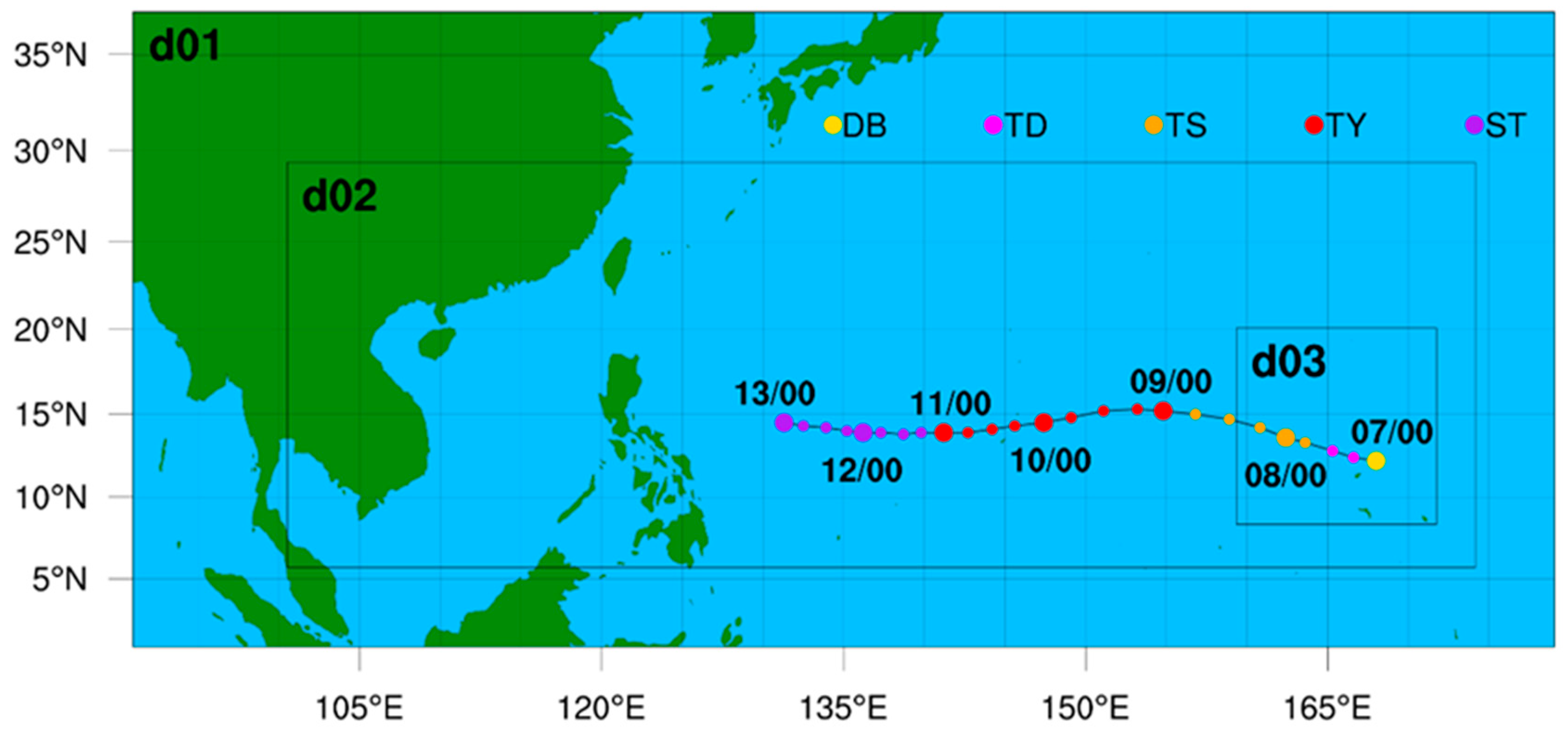
Mangkhut formed over the western North Pacific about 2330 km east of Guam on 7 September, moved westwards quickly, and intensified gradually in the following few days [17,19]. Mangkhut developed into a super typhoon on 11 September. It turned to the northwest on 14 September, reaching its peak intensity before making landfall over Luzon with an estimated maximum sustained wind of 250 km h−1 near the center. Mangkhut weakened after crossing the northern part of Luzon and continued to track northwestwards quickly across the northern part of the South China Sea towards the coast of Guangdong. Mangkhut weakened into a severe typhoon on the morning of 16 September and made landfall in the vicinity of Taishan in Guangdong before dusk. It then moved into the western part of Guangdong and weakened further. Mangkhut degenerated into an area of low pressure over Guangxi the next night. In this study, we focus on the intensification period: from 0000 UTC (Universal Time Coordinated) 7 September to 0000 UTC 13 September 2018, and the track and intensity in this period can be found in Figure 1.
2.2. Experimental Design
The Advanced Research WRF model version 4.0 developed by the US National Center of Atmospheric Research (NCAR) was used for Typhoon Mangkhut simulation. A two-way interactive, three-level nested grid configuration with a track-following moving-nest option was employed. Figure 1 shows the setting of model domains.
The domains have 27, 9, and 3 km horizontal resolution and 342 × 153, 856 × 292, and 433 × 424 grid points, respectively. A total of 33 vertical levels were configured, and the pressure at the uppermost layer was 50 hPa. The initial and lateral boundary conditions were obtained from the fifth-generation European Centre for Medium-Range Weather Forecasts (ECMWF) atmospheric reanalysis of the global climate (ERA5) dataset at a resolution of 0.25° × 0.25°. ERA5 is a widely used dataset for the initial and boundary condition in numerical simulation because of its high resolution of 0.25° × 0.25°, which can provide ideal initial and boundary conditions for numerical simulations [20,21,22]. Additionally, ERA5’s 0.25° resolution is close to the 27 km resolution of the outermost domain in our simulation, which minimizes the error during the reguiding of the initial and boundary condition preparation. Therefore, ERA5 is used in this study. The ERA5 reanalysis data of wind, specific humidity, temperature, and surface flux were also used to assess the model performance. The TC best track from the Joint Typhoon Warning Center (JTWC) was used for evaluating the simulated TC track and intensity.
All the experiments started at 0000 UTC 7 September and ended at 0000 UTC 13 September 2018, covering the intensification period of Typhoon Mangkhut. The first 6 h of integration (i.e., from 0000 UTC to 0006 UTC 7th September 2018) served as the spin-up period, and the results in this period are not investigated.
The model’s physics options were the same for all three domains, except that cumulus parameterization was only used in the 27 km horizontal resolution domain. Physical parameterization options included the Eta (Ferrier) microphysics scheme [23] and the Kain–Fritsch cumulus parameterization scheme [24], the Unified Noah land surface model [25], the Rapid Radiative Transfer longwave radiation scheme (RRTM) [26], the Dudhia shortwave radiation scheme [27], the Mellor–Yamada–Nakanishi–Niino Level 2.5 (MYNN2) [28,29], and the Revised MM5 surface layer scheme [30].
It is noted that the choice of the planetary boundary layer (PBL) and surface layer parameterization scheme is based on our recent work (Ye et al., in preparation), where we found that among the 7 most widely used PBL parameterization schemes, the MYNN2 produced better simulation for the distribution and variation of PBL eddy diffusivity, which is closer to observation, and here, the MYNN2 PBL scheme is coupled to the Revised MM5 surface layer scheme.
2.3. Description of Air–Sea Flux Parameterization in WRF Version 4.0
In Advanced Research WRF, it allows users to change air–sea fluxes formulation through the “namelist” option isftcflx. The revised MM5 surface layer scheme in WRF version 4.0 uses three options for calculating the roughness lengths and air–sea flux. In this study, we conducted a series of sensitivity experiments with 3 different air–sea flux parameterization schemes, respectively. The description is considered comprehensively in WRF version 4.0 code and detailed description is in Green and Zhang [4], Kueh et al. [6], and Alimohammadi et al. [14].
2.3.1. Option 0 (Isftcflx = 0)
Option 0 (isftcflx = 0) is the default option for air–sea flux (or surface roughness) parameterization in WRF Version 4.0. In this option, the momentum roughness length over water is based upon Charnock [31] and adds an upper limit, as in option 1 and 2.
where α = 0.0185 is the Charnock coefficient, is the frictional velocity, and g is the gravitational acceleration. Additionally, the constant value of 1.5 × 10⁻⁵ is used for the kinematic viscosity of air. The Charnock expression relates the aerodynamic roughness length to friction velocity for describing the gross effect of wavy sea surface induced by wind stress, and the viscous term describes roughness behavior under smooth flow conditions [6]. In the case of the momentum roughness length monotonic increasing with wind speed, option 0 adds an upper limit as in options 1 and 2 from WRF version 3.9.
The heat and moisture roughness lengths for option 0 over water are based upon Fairall et al. [32] and expressed as a function of the roughness Reynolds number, with a lower limit of 2.0 × 10⁻⁹ and an upper limit of 1.0 × 10⁻⁴:
where is the roughness Reynolds number, and is the kinematic viscosity of air as a function of air temperature for the calculation [6]. The heat roughness length is set to equal to moisture roughness length . The upper limit of 1.0 × 10⁻⁴ keeps the heat and moisture roughness length constant at extreme wind speeds, whereas the lower limit of 2.0 × 10⁻⁹ is implemented to prevent the model from blowing up.
2.3.2. Option 1 (Isftcflx = 1)
Recent field observations and laboratory experiments showed that is saturated at hurricane wind speed [8,33]. For option 1 (isftcflx = 1), the momentum roughness length is given by a blend of two roughness length formulas [4]:
where is again the Charnock [31] expression plus a viscous term, with Charnock coefficient α = 0.011. is the exponential expression from Davis et al. [9] plus a viscous term, with a constant kinematic viscosity = 1.5 × 10⁻⁵. The two roughness length formulas are combined using a weight function , with a lower limit of 2.0 × 10⁻⁹ and an upper limit of 1.0 × 10⁻⁴ on . The lower and upper limits on are adapted from Davis et al. [9], with a slightly different value of the lower limit. The upper limit is used to prevent a monotonic increase in and at high wind conditions. Additionally, leveling-off of at high wind speed suggests a decline in the efficiency of the exchange of momentum across the air–sea interface.
For the heat and moisture roughness lengths, based on Large and Pond [34], option 1 sets and as constants of 10−4 m for all wind speeds, as:
2.3.3. Option 2 (Isftcflx = 2)
For the momentum roughness length, option 2 (isftcflx = 2) uses the same formulation as option 1. Additionally, the heat and moisture roughness lengths are expressed based on the formula proposed by Brutsaert [35]:
where is the roughness Reynolds number, and is the kinematic viscosity of air. k is the von Karman constant, Pr is the Prandtl number, and Sc is the Schmidt number, and Garratt [36] is used with values of k = 0.40, Pr = 0.71, and Sc = 0.60.
A brief description of the sensitivity experiments is in Table 1, and the relationship between roughness length (or exchange coefficient) and wind speed for different options is in Figure 2. Additionally, these 3 air–sea flux parameterization schemes in revised MM5 stay unchanged from WRF version 3.9 to 4.3, released in 2022.
Figure 2 compared the theoretical results of the roughness length and surface exchange coefficient from 3 surface flux parameterization schemes in the WRF version 4.0 model. For the roughness length in Figure 2a, specifically for the momentum roughness length (thick solid line), OPT1 is the same as OPT2, and all of three have the same upper limit; for the thermal roughness length (thin solid line) and the vapor roughness length (dashed line), OPT1 is greater than OPT0 and OPT2. The surface exchange coefficient is calculated from the roughness length, and for the surface exchange coefficient in Figure 2b, OPT1 is the same as OPT2 for the drag coefficient (thick solid line), and the 3 all have the same upper limit. For the heat exchange coefficient (thin solid line) and water vapor exchange coefficient (dashed line), OPT1 is greater than OPT0 and OPT2. Thus, for the exchange coefficient ratio in Figure 2c, OPT1 is greater than OPT0 and OPT2 for the ratio of (thin solid line) and (dashed line), and in the high wind speed, OPT0 is greater than OPT2.
3. Results
3.1. TC Track and Intensity
In this subsection, we focused on the results of the simulated TC track and intensity for three different air–sea flux schemes for Typhoon Mangkhut during the TC intensification to verify the simulation.
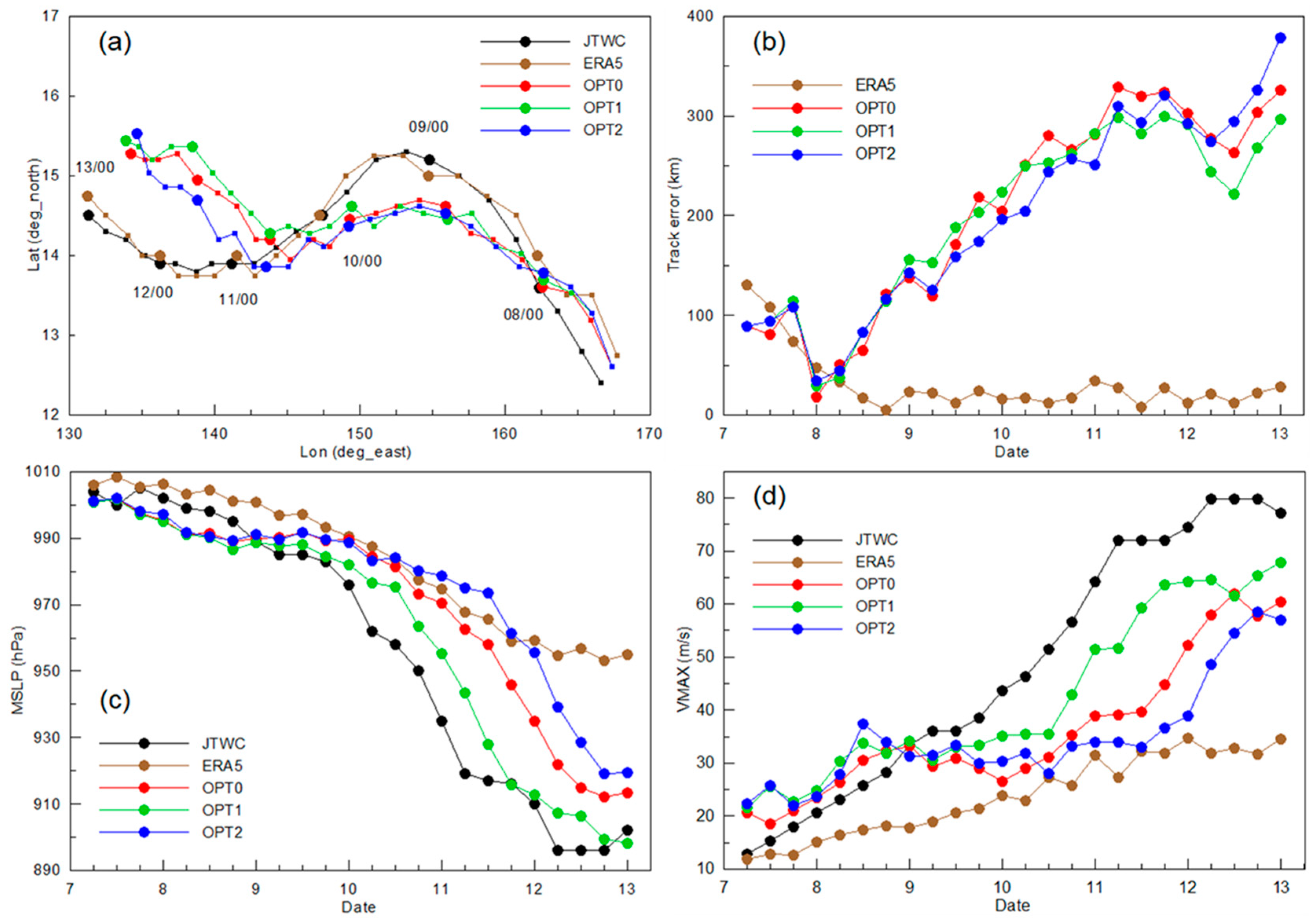
Figure 3a,b shows that the simulated tracks of the three air–sea flux schemes are similar and generally reproduce the westward movement of Typhoon Mangkhut from the JTWC best track. Specifically, from the 7th to 9th September, the simulated tracks of the three schemes were very close, and then the track errors of the three schemes began to gradually increase. Overall, the simulated track was very close. It indicates that the simulated track is not very sensitive to the different air–sea flux scheme, which is consistent with the results in Green and Zhang [4]. It might be related to using the same PBL scheme and surface layer scheme.
For simulated TC intensity, Figure 3c,d further compares the time series of the minimum central sea level pressure (MSLP) and the maximum sustained wind speed (VMAX) of 3 schemes. Compared with the JTWC best track data, the three numerical simulations captured the variation trends of MSLP and VMAX, although an underestimation and difference were found in simulated TC intensity for the three schemes. In the first 3 days until 0000 UTC 10 September, the simulation difference of MSLP and VMAX in the experiments was very small. After that, differences started to show. Seen from the parameter of MSLP, it can be found that OPT1 generally captured the rapid intensification processes from 1800 UTC 9 September to 0600 UTC 11 September, followed by OPT1, while OPT2 showed weaker intensification rates. While looking at the parameter of VMAX, a similar pattern can be found. During the rapid intensification processes at the end of the simulation, among the three simulations, OPT1 had the largest VMAX, followed by OPT0, whereas OPT2 was smaller than the JTWC’s VMAX. The simulated results of TC intensity demonstrate the evident sensitivity of intensity to the air–sea flux scheme, which is consistent with the conclusion in Green and Zhang [4]. According to theoretical results of exchange coefficient in Figure 2, at high wind speed, OPT1 has the larger and with the same and larger and . The ratio of and correspond to the TC intensity. In the next subsection, we further study the relationship between TC intensity and exchange coefficient based on the simulated results in the three simulations.
3.2. Surface Exchange Coefficient
The intensity variations among different air–sea flux (or surface roughness) schemes become evident in the TC intensification stage because of the dependence of wind speed on surface exchanges of momentum and moisture enthalpy [37]. In this subsection, we analyze the variation of the simulated surface exchange coefficient with the 10 m wind speed among the three schemes at the TC peak intensity of 1200 UTC 12th September, at which TC reached mature stage.
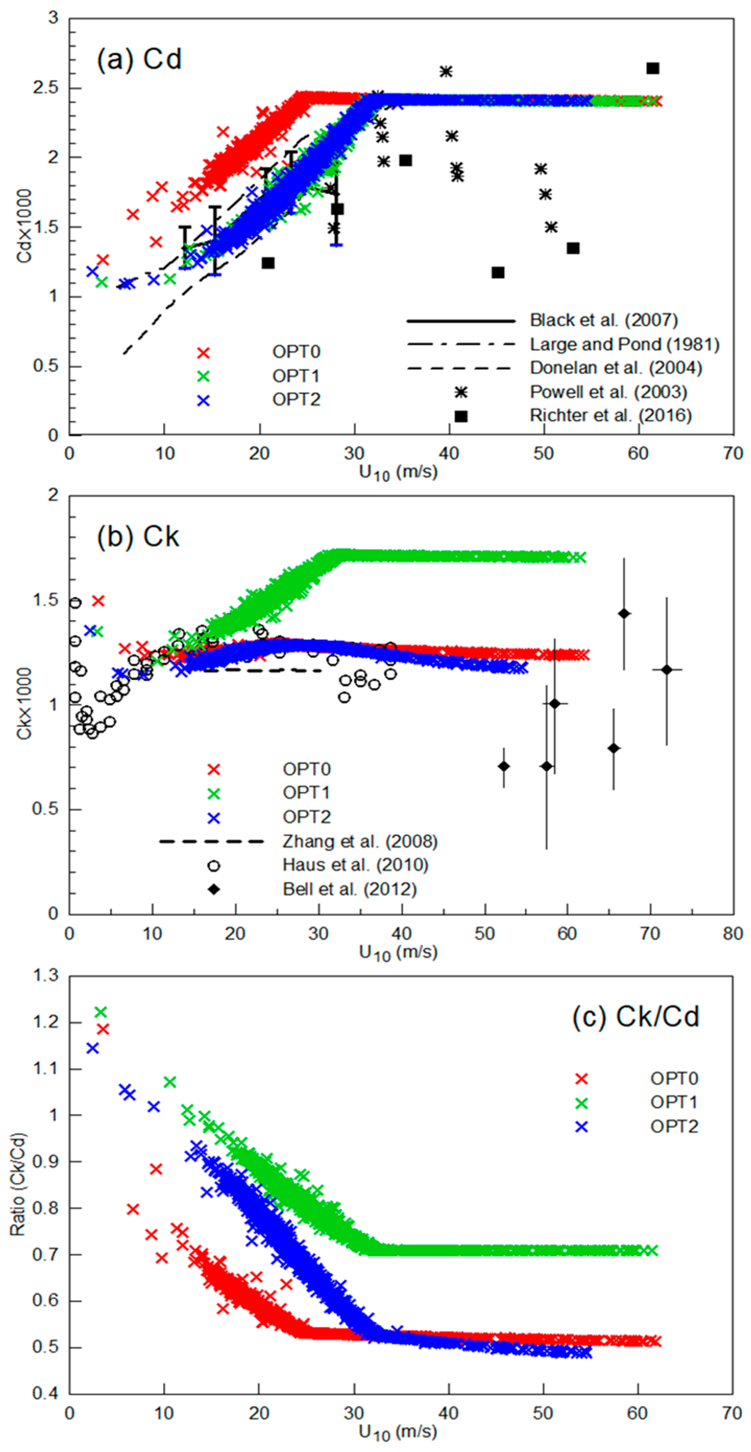
In Figure 4, the simulated values for and are similar with the theoretical values in Figure 2. In Figure 4a, the of the three schemes all increased initially with increasing wind speed until high wind, and the of OPT0 reached saturation slightly earlier than the of OPT1 and OPT2. Additionally, the of the three schemes share the same upper limit (about 2.4 × 10⁻³) under high wind speed (beyond about 33 m s−1).
In Figure 4b, the of OPT0 is nearly unchanged with increasing wind speed. Similar to , the of OPT1 increased initially with increasing wind speed below 33 m s−1 and saturated thereafter. Additionally, the of OPT2 increased slowly with increasing wind speed below 33 m s−1 and thereafter tended to decrease slightly. Among the three simulations, the of OPT1 is significantly larger than the of OPT0 and OPT2, and in high wind speed, the of OPT0 is slightly larger than the of OPT2.
Due to the same upper limit in for all three schemes, the difference in affects the differences in . In Figure 4c, the of OPT1 is the largest, and the of OPT0 is slightly larger than the of OPT2 when wind speed exceeds 33 m s−1. Emanuel [11] suggested that in real hurricanes lies in the range 0.75–1.5. Among the three schemes, only OPT1 follows this rule (Figure 4c). It is noted that the of OPT1 is significantly larger than observation results from previous studies [38,39,40].
Since maximum wind speed is strongly sensitive to [11], the decrease in (generally tends to reduce the energy loss) and increase in (thus more energy gain) have greater potential to yield a stronger storm [6]. Correspondingly, in this study, the magnitude of is consistent with the simulated TC intensity relationship for the three schemes because differences in and affect surface energy transport and influence the storm intensification by WISHE type of feedback [4,13,37].
3.3. Surface Flux
As mentioned above, different air–sea flux (or surface roughness) schemes produce different and values, and and determine the surface enthalpy flux and momentum flux, respectively [43]. The surface enthalpy flux is the main source of energy for TC development, while surface momentum flux is the main sink of TC energy. In this subsection, we look into the simulated result of surface fluxes in numerical experiments.
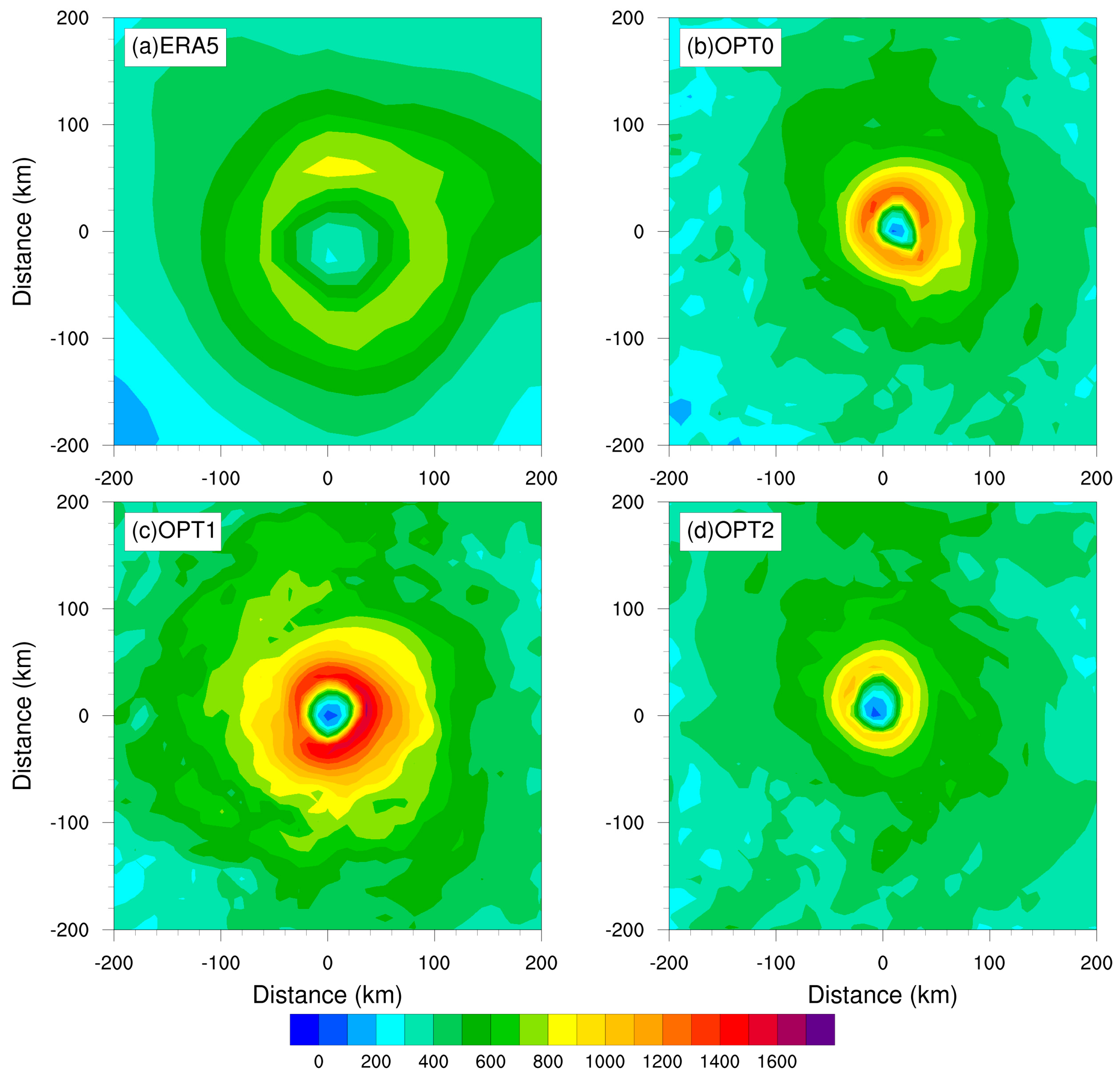
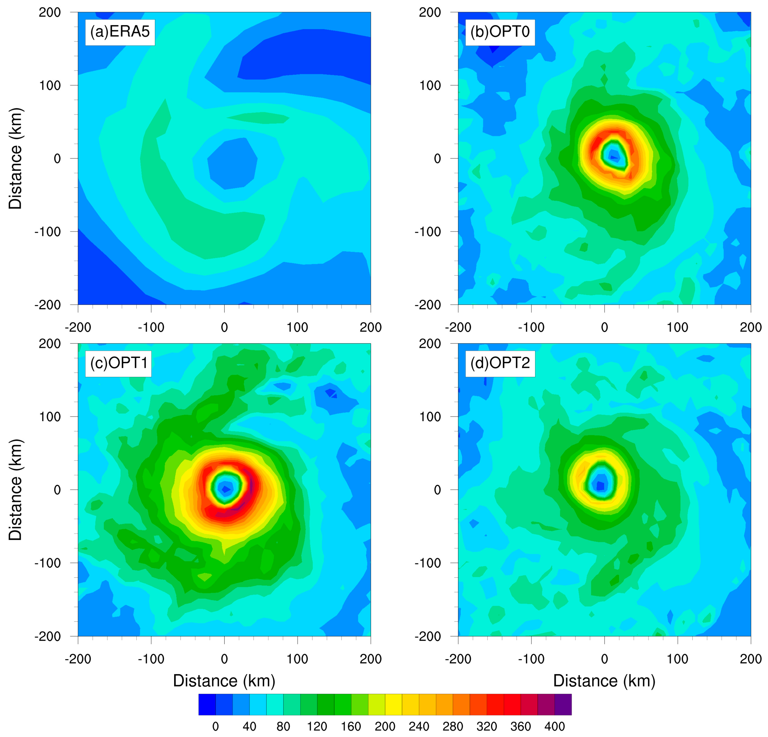
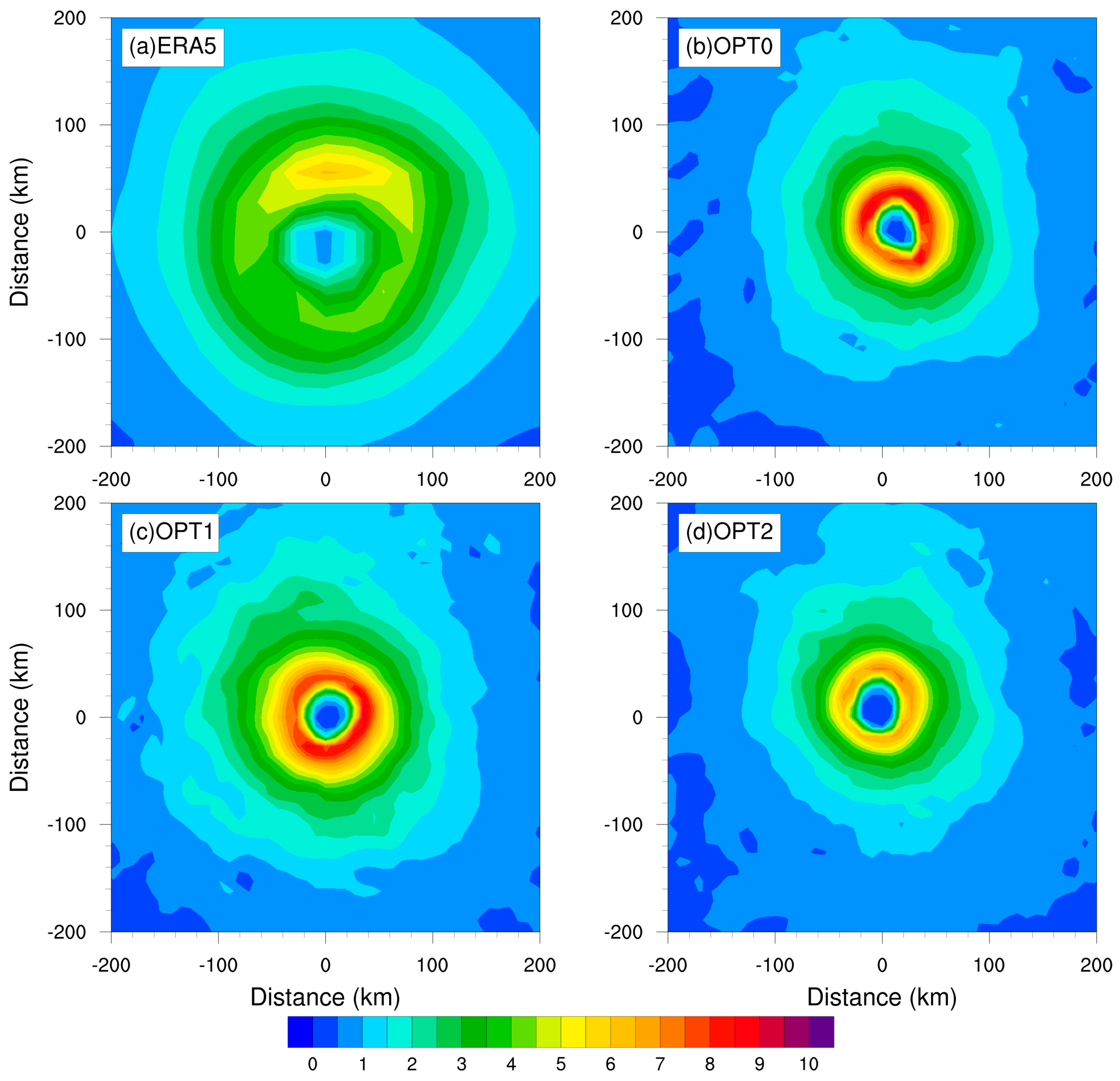
Figure 5, Figure 6 and Figure 7 plot the distribution of surface latent heat, sensible heat, and momentum flux simulated by different sea–air flux schemes within a radius of 500 km at 1200 UTC 12, September 2018, which represents mature TC. Additionally, ERA5 reanalysis data are used here for comparison. Consistent with TC intensity results in Figure 3, surface fluxes of ERA5 are significantly smaller than simulated surface fluxes from three options, although the distributions of surface fluxes from ERA5 and simulations are similar. Figure 5 and Figure 6 show that sensible heat fluxes are smaller than latent heat fluxes, which is consistent with those derived from field measurements (e.g., [4,38]). Additionally, whether latent and sensible heat flux or momentum flux, surface flux is the weakest in the TC center and gradually increases outward from the TC eye, reaching its maximum near the eyewall.
Consistent with the magnitude relationship of TC intensity, OPT1 produced the largest latent flux and sensibility, followed by OPT0 and OPT2. This better simulation of TC intensity by OPT0 can be attributed to the steady increase in latent flux for high wind speed. The larger latent heat flux transfer results in stronger moist convection, thereby leading to stronger TC intensity for simulation through thermo-dynamical interactions [37]. Similarly, OPT1 produced larger momentum flux than OPT0 and OPT2, since momentum flux is influenced by wind speed. Overall, the difference in momentum is relatively small due to the same peak for the three schemes.
In general, although sharing the same upper limit in as OPT0 and OPT2, OPT1 has much larger than the other two options, which leads to larger enthalpy flux, and especially latent heat flux, and thus stronger TC intensity.
3.4. TC Wind Field
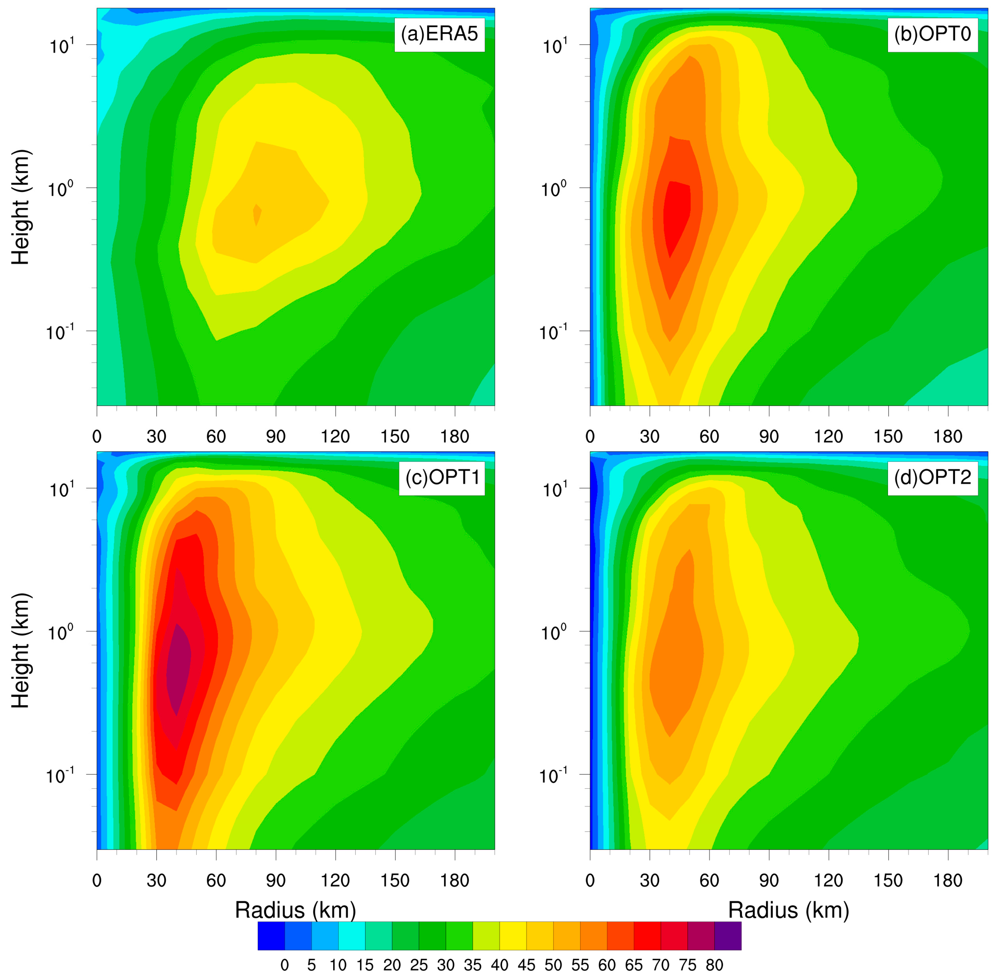
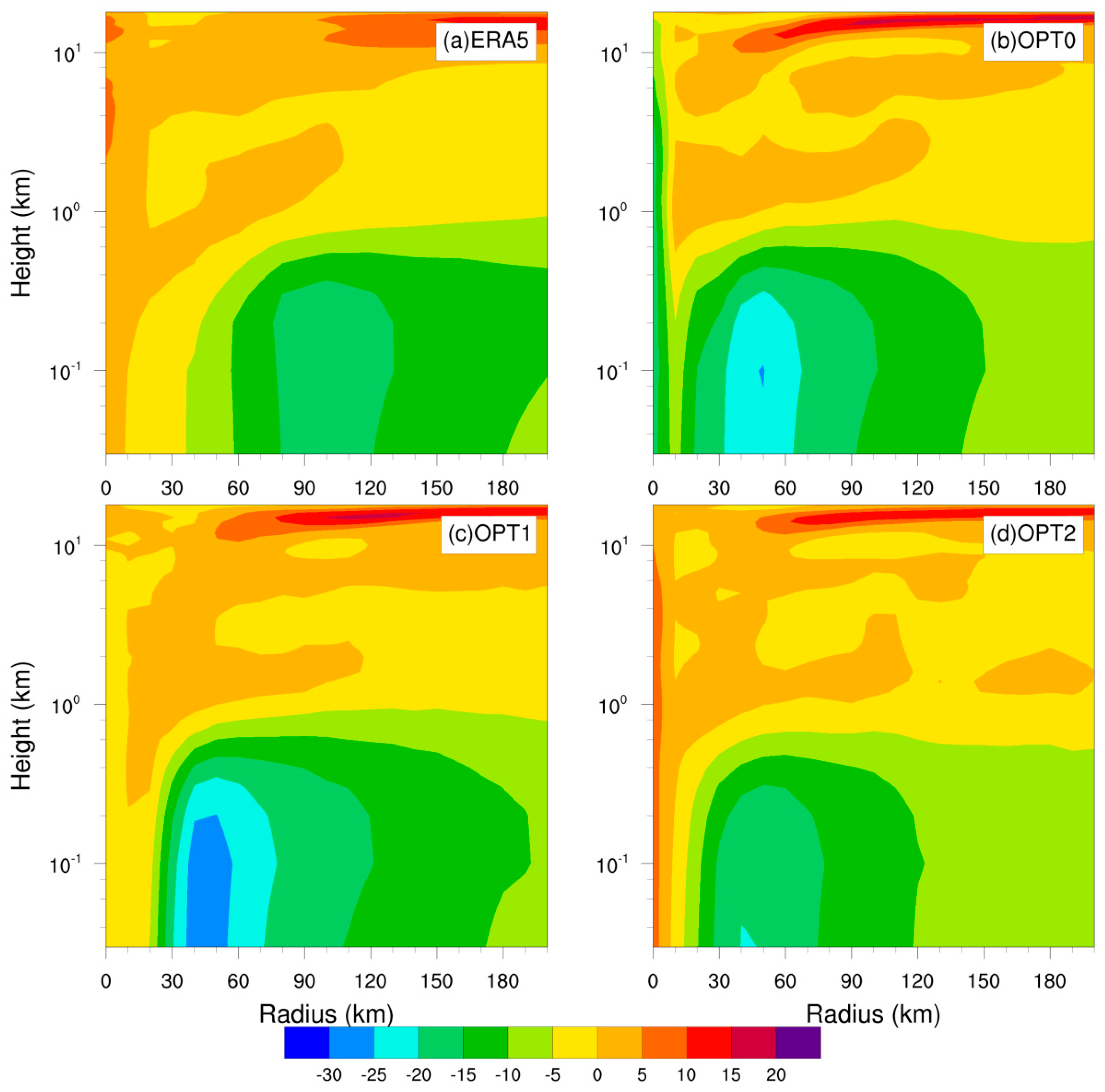
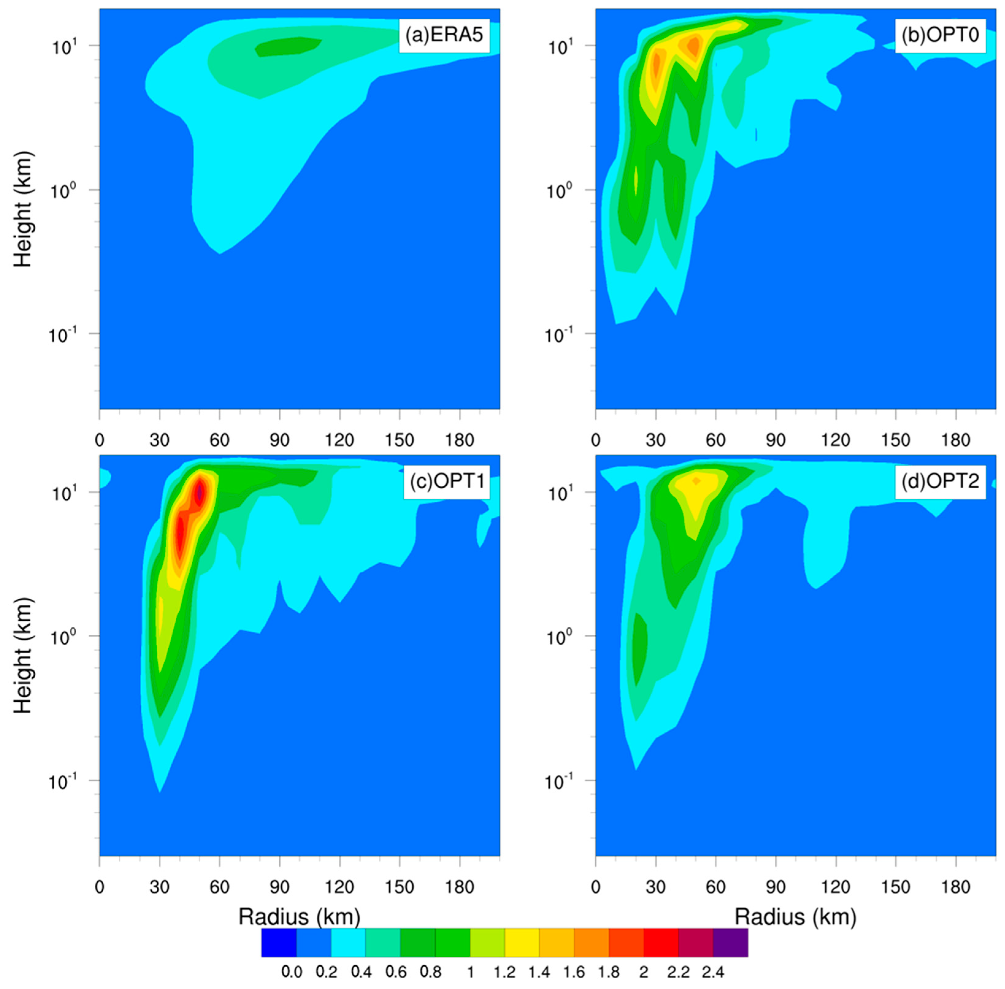
In this subsection, the height–radius distribution of azimuthally averaged tangential wind, radial wind, and upward vertical wind within 200 km from the TC center 1200 UTC 12 September simulated by the three schemes are analyzed. Similar with the last subsection, 1200 UTC 12 September is chosen to represent the TC mature stage when the simulated TC reached its peak intensity. Additionally, ERA5 reanalysis data are used as a reference to compare the simulation results. Although ERA5 generally underestimates the TC intensity, it provides an effective reference for TC size [44]. Consistent with TC intensity results in Figure 3, the wind speed of ERA5 is significantly weaker than the simulated wind speed from the three options. For TC size (i.e., radius of maximum tangential wind speed) in Figure 8, the three options simulate a similar TC size, which is smaller than ERA5’s TC size.
Radius–height plots of the tangential, radial, and vertical winds at 1200 UTC 12 September (Figure 8, Figure 9 and Figure 10) indicate that the different air–sea flux schemes yield the same general wind structure, which is consistent with results in Green and Zhang [4], albeit with some differences in the magnitude of peak wind speed.
OPT1 has the strongest wind speed, including a peak tangential wind speed greater than 75 m s−1, peak radial inflow velocity (within boundary layer) greater than 25 m s−1, and peak upward velocity (along eyewall) greater than 2.2 m s−1. Next, OPT0 has stronger wind than OPT2, with peak tangential wind speed greater than 65 m s−1, peak radial inflow velocity (within boundary layer) about 25 m s−1, and peak upward velocity (along eyewall) about 1.6 m s−1. Greater tangential wind corresponds to stronger TC, whereas stronger inflow within the boundary layer and updrafts around the eyewall lead to stronger TC. The magnitude relationship of peak wind speed corresponds to the TC intensity, , and surface latent flux.
For better TC intensification simulation by OPT1, although sharing the same upper limit for , the larger of OPT1 produces greater latent flux (and sensible flux) and stronger wind field, including stronger radial inflow (boundary layer) and updrafts (around eyewall), which leads to stronger storms.
4. Conclusions
In this study, using the Advanced Research WRF version 4.0 model, a series of numerical experiments for Typhoon Mangkhut are performed to examine the sensitivity of TC intensification simulation with three different air–sea flux (or surface roughness) parameterization schemes (isftcflx options), including OPT0, OPT1, and OPT2. The major findings can be summarized as follows:
(1) 3 Air–sea schemes simulate and basically reproduce the TC track and intensity of observation, and simulated exchange coefficients are consistent with theoretical results.
(2) Although using the same upper limit of as OPT0 and OPT2, OPT1 has much larger than the other two options, which leads to larger latent heat (and sensible heat) flux and produces stronger inflow (within boundary layer) and updrafts (around eyewall), and thus stronger TC intensity. Meanwhile, the results that larger corresponds with stronger TC in the mature stage are consistent with Emanuel’s PI theory.
(3) Although producing the better TC intensity simulation, as a matter of fact, the in OPT1 is evidently larger than the from previous studies. In brief, more reasonable air–sea flux parameterization can improve TC intensity simulation to a certain extent.
In future, we need to conduct further work on air–sea flux parameterization and observation of TC intensification, in order to produce more accurate intensity forecasts and accurate exchange coefficient simulation under TC condition.
Author Contributions
Conceptualization, L.Y. and Y.L.; methodology, L.Y.; software, L.Y.; validation, L.Y.; formal analysis, L.Y. and Y.L.; investigation, L.Y. and Y.L.; resources, L.Y.; data curation, L.Y.; writing—original draft preparation, L.Y.; writing—review and editing, L.Y., Y.L. and Z.G.; visualization, L.Y.; supervision, Y.L. and Z.G.; project administration, Y.L. and Z.G.; funding acquisition, Y.L. All authors have read and agreed to the published version of the manuscript.
Funding
This study was supported by the National Natural Science Foundation of China (42075072), the Innovation Group Project of Southern Marine Science and Engineering Guangdong Laboratory (Zhuhai) (311021008), and Postgraduate Research and Practice Innovation Program of Jiangsu Province (KYCX22_1152).
Institutional Review Board Statement
Not applicable.
Informed Consent Statement
Not applicable.
Acknowledgments
The numerical calculations in this paper have been done on the supercomputing system in the Supercomputing Center of Nanjing University of Information Science & technology.
Conflicts of Interest
The authors declare no conflict of interest.
References
- Glenn, S.M.; Miles, T.N.; Seroka, G.N.; Xu, Y.; Forney, R.K.; Yu, F.; Roarty, H.; Schofield, O.; Kohut, J. Stratified coastal ocean interactions with tropical cyclones. Nat. Commun. 2016, 7, 10887. [Google Scholar] [CrossRef] [PubMed] [Green Version]
- Seroka, G.; Miles, T.; Xu, Y.; Kohut, J.; Schofield, O.; Glenn, S. Hurricane Irene Sensitivity to Stratified Coastal Ocean Cooling. Mon. Weather Rev. 2016, 144, 3507–3530. [Google Scholar] [CrossRef]
- Black, P.G.; D’Asaro, E.A.; Drennan, W.M.; French, J.R.; Niiler, P.P.; Sanford, T.B.; Terrill, E.J.; Walsh, E.J.; Zhang, J.A. Air–sea exchange in hurricanes: Synthesis of observations from the Coupled Boundary Layer Air–Sea Transfer experiment. Bull. Am. Meteorol. Soc. 2007, 88, 357–374. [Google Scholar] [CrossRef] [Green Version]
- Green, B.W.; Zhang, F. Impacts of air–sea flux parameterizations on the intensity and structure of tropical cyclones. Mon. Weather Rev. 2013, 141, 2308–2324. [Google Scholar] [CrossRef] [Green Version]
- Green, B.W.; Zhang, F. Sensitivity of tropical cyclone simulations to parametric uncertainties in air–sea fluxes and implications for parameter estimation. Mon. Weather Rev. 2014, 142, 2290–2308. [Google Scholar] [CrossRef]
- Kueh, M.T.; Chen, W.M.; Sheng, Y.F.; Lin, S.C.; Wu, T.R.; Yen, E.; Tsai, Y.L.; Lin, C.Y. Effects of horizontal resolution and air-sea flux parameterization on the intensity and structure of simulated Typhoon Haiyan. Nat. Hazards Earth Syst. Sci. 2019, 19, 1509–1539. [Google Scholar] [CrossRef] [Green Version]
- Rizza, U.; Canepa, E.; Miglietta, M.M.; Passerini, G.; Morichetti, M.; Mancinelli, E.; Virgili, S.; Besio, G.; De Leo, F.; Mazzino, A. Evaluation of drag coefficients under medicane conditions: Coupling waves, sea spray and surface friction. Atmos. Res. 2021, 247, 105207. [Google Scholar] [CrossRef]
- Powell, M.D.; Vickery, P.J.; Reinhold, T. Reduced drag coefficient for high wind speeds in tropical cyclones. Nature 2003, 422, 279–283. [Google Scholar] [CrossRef]
- Davis, C.; Wang, W.; Chen, S.S.; Chen, Y.; Corbosiero, K.; DeMaria, M.; Dudhia, J.; Holland, G.; Klemp, J.; Michalakes, J.; et al. Prediction of landfalling hurricanes with the Advanced Hurricane WRF model. Mon. Weather Rev. 2008, 136, 1990–2005. [Google Scholar] [CrossRef] [Green Version]
- Emanuel, K.A. An air–sea interaction theory for tropical cyclones. Part I: Steady-state maintenance. J. Atmos. Sci. 1986, 43, 585–604. [Google Scholar] [CrossRef]
- Emanuel, K.A. Sensitivity of tropical cyclones to surface exchange coefficients and a revised steady-state model incorporating eye dynamics. J. Atmos. Sci. 1995, 52, 3969–3976. [Google Scholar] [CrossRef]
- Chen, Y.; Zhang, F.; Green, B.W.; Yu, X. Impacts of ocean cooling and reduced wind drag on hurricane Katrina (2005) based on numerical simulations. Mon. Weather Rev. 2018, 146, 287–306. [Google Scholar] [CrossRef]
- Greeshma, M.; Srinivas, C.V.; Hari Prasad, K.B.R.R.; Baskaran, R.; Venkatraman, B. Sensitivity of tropical cyclone predictions in the coupled atmosphere–ocean model WRF-3DPWP to surface roughness schemes. Meteorol. Appl. 2019, 26, 324–346. [Google Scholar] [CrossRef] [Green Version]
- Alimohammadi, M.; Malakooti, H.; Rahbani, M. Comparison of momentum roughness lengths of the WRF-SWAN online coupling and WRF model in simulation of tropical cyclone Gonu. Ocean Dyn. 2020, 70, 1531–1545. [Google Scholar] [CrossRef]
- Nystrom, R.G.; Chen, X.; Zhang, F.; Davis, C.A. Nonlinear impacts of surface exchange coefficient uncertainty on tropical cyclone intensity and air-sea interactions. Geophys. Res. Lett. 2020, 47, e2019GL085783. [Google Scholar] [CrossRef]
- Nystrom, R.G.; Rotunno, R.; Davis, C.A.; Zhang, F. Consistent impacts of surface enthalpy and drag coefficient uncertainty between an analytical model and simulated tropical cyclone maximum intensity and storm structure. J. Atmos. Sci. 2020, 77, 3059–3080. [Google Scholar] [CrossRef]
- He, Y.C.; He, J.Y.; Chen, W.C.; Chan, P.W.; Fu, J.Y.; Li, Q. Insights from Super Typhoon Mangkhut (1822) for wind engineering practices. J. Wind Eng. Ind. Aerodyn. 2020, 203, 104238. [Google Scholar] [CrossRef]
- Yang, J.; Li, L.; Zhao, K.; Wang, P.; Wang, D.; Sou, I.M.; Yang, Z.; Hu, J.; Tang, X.; Mok, K.M.; et al. A Comparative Study of Typhoon Hato (2017) and Typhoon Mangkhut (2018)–Their Impacts on Coastal Inundation in Macau. J. Geophys. Res. Oceans 2019, 124, 9590–9619. [Google Scholar] [CrossRef]
- He, Q.; Zhang, K.; Wu, S.; Zhao, Q.; Wang, X.; Shen, Z.; Li, L.; Wan, M.; Liu, X. Real-Time GNSS-Derived PWV for Typhoon Characterizations: A Case Study for Super Typhoon Mangkhut in Hong Kong. Remote Sens. 2020, 12, 104. [Google Scholar] [CrossRef] [Green Version]
- Li, D.; Staneva, J.; Bidlot, J.R.; Grayek, S.; Zhu, Y.; Yin, B. Improving Regional Model Skills During Typhoon Events: A Case Study for Super Typhoon Lingling Over the Northwest Pacific Ocean. Front. Mar. Sci. 2021, 8, 613913. [Google Scholar] [CrossRef]
- Gevorgyan, A. Convection-permitting simulation of a heavy rainfall event in Armenia using the WRF model. J. Geophys. Res. Atmos. 2018, 123, 11,008–11,029. [Google Scholar] [CrossRef]
- Wu, J.F.; Xue, X.H.; Hoffmann, L.; Dou, X.K.; Li, H.M.; Chen, T.D. A case study oftyphoon-induced gravity wavesand the orographic impactsrelated to Typhoon Mindulle (2004) over Taiwan. J. Geophys. Res. Atmos. 2015, 120, 9193–9207. [Google Scholar] [CrossRef] [Green Version]
- Rogers, E.; Black, T.; Ferrier, B.; Lin, Y.; Parrish, D.; DiMego, G. Changes to the NCEP Meso Eta analysis and forecast system: Increase in resolution, new cloud microphysics, modified precipitation assimilation, and modified 3DVAR analysis. NWS Tech. Proced. Bull. 2001, 488, 15. [Google Scholar]
- Kain, J.S. The Kain–Fritsch convective parameterization: An update. J. Appl. Meteorol. 2004, 43, 170–181. [Google Scholar] [CrossRef]
- Tewari, M.; Chen, F.; Wang, W.; Dudhia, J.; LeMone, M.A.; Mitchell, K.; Ek, M.; Gayno, G.; Wegiel, J.; Cuenca, R.H. Implementation and verification of the unified NOAH land surface model in the WRF model. In Proceedings of the 20th Conference on Weather Analysis and Forecasting/16th Conference on Numerical Weather Prediction, Seattle, WA, USA, 14 January 2004; pp. 11–15. [Google Scholar]
- Mlawer, E.J.; Taubman, S.J.; Brown, P.D.; Iacono, M.J.; Clough, S.A. Radiative transfer for inhomogeneous atmospheres: RRTM, a validated correlated–k model for the longwave. J. Geophys. Res. 1997, 102, 16663–16682. [Google Scholar] [CrossRef] [Green Version]
- Dudhia, J. Numerical study of convection observed during the Winter Monsoon Experiment using a mesoscale two–dimensional model. J. Atmos. Sci. 1989, 46, 3077–3107. [Google Scholar] [CrossRef]
- Nakanishi, M.; Niino, H. An improved Mellor–Yamada level 3 model: Its numerical stability and application to a regional prediction of advecting fog. Bound. -Layer Meteorol. 2006, 119, 397–407. [Google Scholar] [CrossRef]
- Nakanishi, M.; Niino, H. Development of an improved turbulence closure model for the atmospheric boundary layer. J. Meteorol. Soc. Jpn. 2009, 87, 895–912. [Google Scholar] [CrossRef] [Green Version]
- Jimenez, P.A.; Dudhia, J.; Gonzalez-Rouco, J.F.; Navarro, J.; Montavez, J.P.; Garcia-Bustamante, E. A revised scheme for the WRF surface layer formulation. Mon. Weather Rev. 2012, 140, 898–918. [Google Scholar] [CrossRef] [Green Version]
- Charnock, H. Wind stress on a water surface. Q. J. R. Meteor. Soc. 1955, 81, 639–640. [Google Scholar] [CrossRef]
- Fairall, C.W.; Bradley, E.F.; Hare, J.E.; Grachev, A.A.; Edson, J.B. Bulk parameterization of air–sea fluxes: Updates and verification for the COARE algorithm. J. Clim. 2003, 16, 571–591. [Google Scholar] [CrossRef]
- Donelan, M.A.; Haus, B.K.; Reul, N.; Plant, W.J.; Stiassnie, M.; Graber, H.C.; Brown, O.B.; Saltzman, E.S. On the limiting aerodynamic roughness of the ocean in very strong winds. Geophys. Res. Lett. 2004, 31, L18306. [Google Scholar] [CrossRef] [Green Version]
- Large, W.G.; Pond, S. Sensible and latent heat flux measurements over the ocean. J. Phys. Oceanogr. 1982, 12, 464–482. [Google Scholar] [CrossRef]
- Brutsaert, W. A theory for local evaporation (or heat transfer) from rough and smooth surfaces at ground level. Water Resour. Res. 1975, 11, 543–550. [Google Scholar] [CrossRef]
- Garratt, J.R. The Atmospheric Boundary Layer; Cambridge University Press: Cambridge, UK, 1992; p. 316. [Google Scholar]
- Nellipudi, N.R.; Yesubabu, V.; Srinivas, C.V.; Vissa, N.K.; Sabique, L. Impact of surface roughness parameterizations on tropical cyclone simulations over the Bay of Bengal using WRF-OML model. Atmos. Res. 2021, 262, 105779. [Google Scholar] [CrossRef]
- Large, W.G.; Pond, S. Open Ocean momentum flux measurements in moderate to strong winds. J. Phys. Oceanogr. 1981, 11, 324–336. [Google Scholar] [CrossRef]
- Zhang, J.A.; Black, P.G.; French, J.R.; Drennan, W.M. First direct measurements of enthalpy flux in the hurricane boundary layer: The CBLAST results. Geophys. Res. Lett. 2008, 35, L14813. [Google Scholar] [CrossRef] [Green Version]
- Haus, B.K.; Jeong, D.; Donelan, M.A.; Zhang, J.A.; Savelyev, I. Relative rates of sea-air heat transfer and frictional drag in very high winds. Geophys. Res. Lett. 2010, 37, L07802. [Google Scholar] [CrossRef]
- Bell, M.M.; Montgomery, M.T.; Emanuel, K.A. Air–sea enthalpy and momentum exchange at major hurricane wind speeds observed during CBLAST. J. Atmos. Sci. 2012, 69, 3197–3222. [Google Scholar] [CrossRef]
- Richter, D.H.; Bohac, R.; Stern, D.P. An Assessment of the Flux Profile Method for Determining Air-Sea Momentum and Enthalpy Fluxes from Dropsonde Data in Tropical Cyclones. J. Atmos. Sci. 2016, 73, 2665–2682. [Google Scholar] [CrossRef]
- Gopalakrishnan, S.G.; Marks, F.; Zhang, J.A.; Zhang, X.; Bao, M.J.W.; Tallapragada, V. A study of the impacts of vertical diffusion on the structure and intensity of the tropical cyclones using the high-resolution HWRF system. J. Atmos. Sci. 2013, 70, 524–541. [Google Scholar] [CrossRef]
- Bian, G.F.; Nie, G.Z.; Qiu, X. How well is outer tropical cyclone size represented in the era5 reanalysis dataset? Atmos. Res. 2021, 249, 105339. [Google Scholar] [CrossRef]
Figure 1.
The location of model-simulated domains and the best track of Mangkhut from JTWC during the simulated period from 0000 UTC 7 to 0000 UTC 13 September 2018. Colored dots are the TC track, and colors indicate the categories of TC intensity (DB: disturbance; TD: tropical depression; TS: tropical storm; TY: typhoon; ST: super typhoon).

Figure 2.
Plots as functions of 10 m wind speed of (a) roughness lengths (thick solid), (thin solid), and (dashed); (b) exchange coefficients (thick solid), (thin solid), and (dashed); (c) exchange coefficient ratios (thin solid) and (dashed), for neutral stability condition. Air–sea flux schemes option 0, option 1, and option 2, colored red, green, and blue, respectively. As stated in the text, some curves are identical: for option 0, and ; for option 1, and ; and between option 1 and option 2, (and thus ) is the same.

Figure 3.
(a) TC track, (b) time series of track error (unit: km), (c) minimum central sea level pressure (MSLP) (unit: hPa), and (d) maximum sustained wind speed (VMAX) (unit: m s−1) from the JTWC best track data; ERA5 reanalysis data and the numerical simulations from 0600 UTC 7 to 0000 UTC 13 September 2018.

Figure 4.
The variation of surface exchange coefficient for (a) , (b) , and (c) ratio of with 10 m wind speed at 1200 UTC 12 September 2018; numerical simulations by OPT0 (in red), OPT1 (in green), and OPT2 (in blue) compared with data from Large and Pond [38], Powell et al. [8], Donelan et al. [33], Black et al. [3], Zhang et al. [39], Haus et al. [40], Bell et al. [41], and Richter et al. [42] (in different black marks).

Figure 5.
Surface latent heat flux (unit: W m−2) of Typhoon Mangkhut from (a) ERA5, (b) OPT0, (c) OPT1, and (d) OPT2 at 1200 UTC 12 September 2018.
Figure 5.
Surface latent heat flux (unit: W m−2) of Typhoon Mangkhut from (a) ERA5, (b) OPT0, (c) OPT1, and (d) OPT2 at 1200 UTC 12 September 2018.

Figure 6.
As in Figure 5 but for surface sensible heat flux (unit: W m−2).
Figure 6.
As in Figure 5 but for surface sensible heat flux (unit: W m−2).

Figure 7.
As in Figure 5 but for surface momentum flux (unit: kg m−1 s−2).
Figure 7.
As in Figure 5 but for surface momentum flux (unit: kg m−1 s−2).

Figure 8.
Height–radius distribution of azimuthally averaged tangential wind (unit: m s−1) from (a) ERA5, (b) OPT0, (c) OPT1, and (d) OPT2 at 1200 UTC 12 September 2018.
Figure 8.
Height–radius distribution of azimuthally averaged tangential wind (unit: m s−1) from (a) ERA5, (b) OPT0, (c) OPT1, and (d) OPT2 at 1200 UTC 12 September 2018.

Figure 9.
As in Figure 8 but for radial wind (unit: m s−1).
Figure 9.
As in Figure 8 but for radial wind (unit: m s−1).

Figure 10.
As in Figure 8 but for upward vertical wind (unit: m s−1).
Figure 10.
As in Figure 8 but for upward vertical wind (unit: m s−1).


Table 1.
Brief description of the sensitivity numerical experiments.
| Experiment Name | Surface Layer Scheme | Air–Sea Flux Scheme | ||
|---|---|---|---|---|
| OPT0 | Revised MM5 | isftcflx = 0 | Charnock [31], Donelan et al. [33] | Fairall et al. [32] |
| OPT1 | Revised MM5 | isftcflx = 1 | Donelan et al. [33] | Large and Pond [34] |
| OPT2 | Revised MM5 | isftcflx = 2 | Donelan et al. [33] | Garratt [36] |
Publisher’s Note: MDPI stays neutral with regard to jurisdictional claims in published maps and institutional affiliations. |
© 2022 by the authors. Licensee MDPI, Basel, Switzerland. This article is an open access article distributed under the terms and conditions of the Creative Commons Attribution (CC BY) license (https://creativecommons.org/licenses/by/4.0/).
Share and Cite
MDPI and ACS Style
Ye, L.; Li, Y.; Gao, Z. Evaluation of Air–Sea Flux Parameterization for Typhoon Mangkhut Simulation during Intensification Period. Atmosphere 2022, 13, 2133. https://doi.org/10.3390/atmos13122133
AMA Style
Ye L, Li Y, Gao Z. Evaluation of Air–Sea Flux Parameterization for Typhoon Mangkhut Simulation during Intensification Period. Atmosphere. 2022; 13(12):2133. https://doi.org/10.3390/atmos13122133
Chicago/Turabian StyleYe, Lei, Yubin Li, and Zhiqiu Gao. 2022. "Evaluation of Air–Sea Flux Parameterization for Typhoon Mangkhut Simulation during Intensification Period" Atmosphere 13, no. 12: 2133. https://doi.org/10.3390/atmos13122133
Note that from the first issue of 2016, this journal uses article numbers instead of page numbers. See further details here.