
Analysis of the Sporadic-E Layer Behavior in Different American Stations during the Days around the September 2017 Geomagnetic Storm

 , , , ,
Abstract
:1. Introduction
2. Data Analysis and Methodology
2.1. The Es Layer Parameters Obtained in Ionograms
2.2. MIRE Mode8
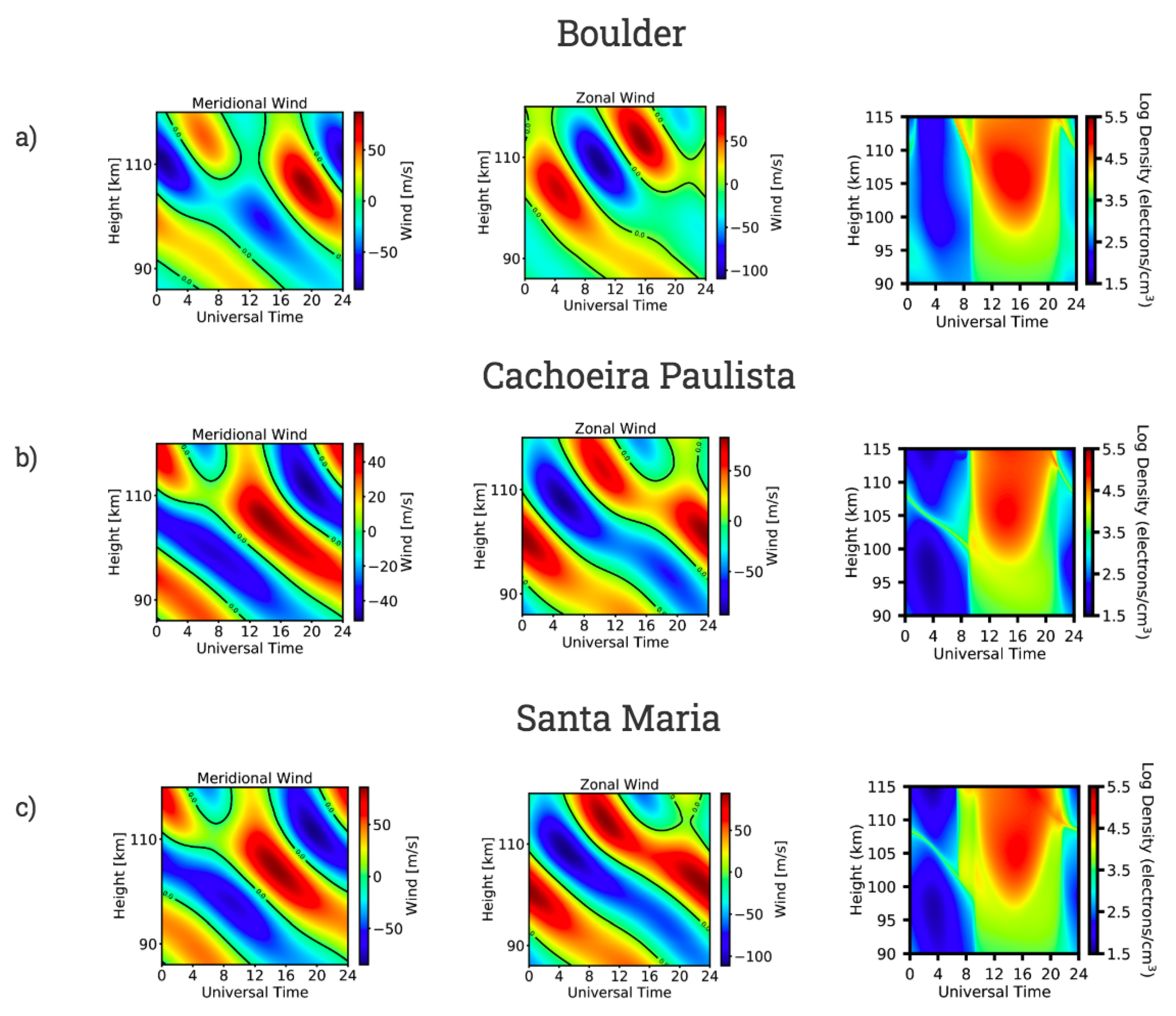
2.3. The Winds Profile
2.4. The Es Layer Detection by Radio Occultation (RO) Technique
3. Results
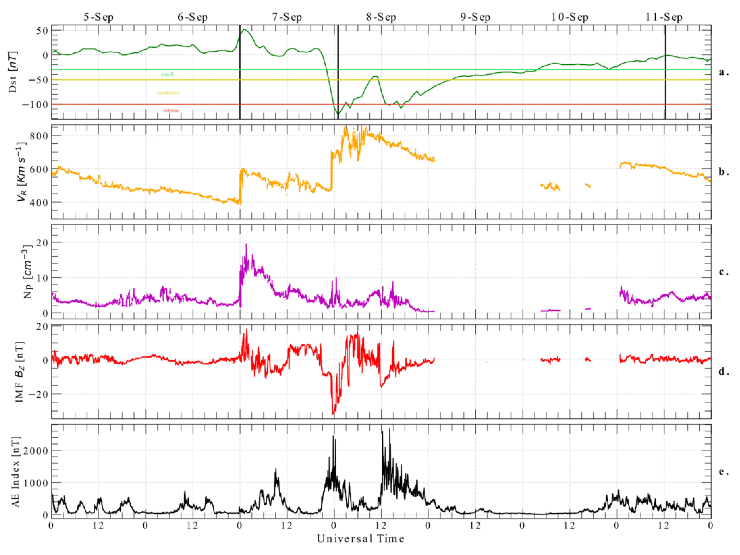
3.1. The 8 September 2017, Geomagnetic Storm
3.2. The Behaviour of the Es Layer Parameters over the American Sector
- (1)
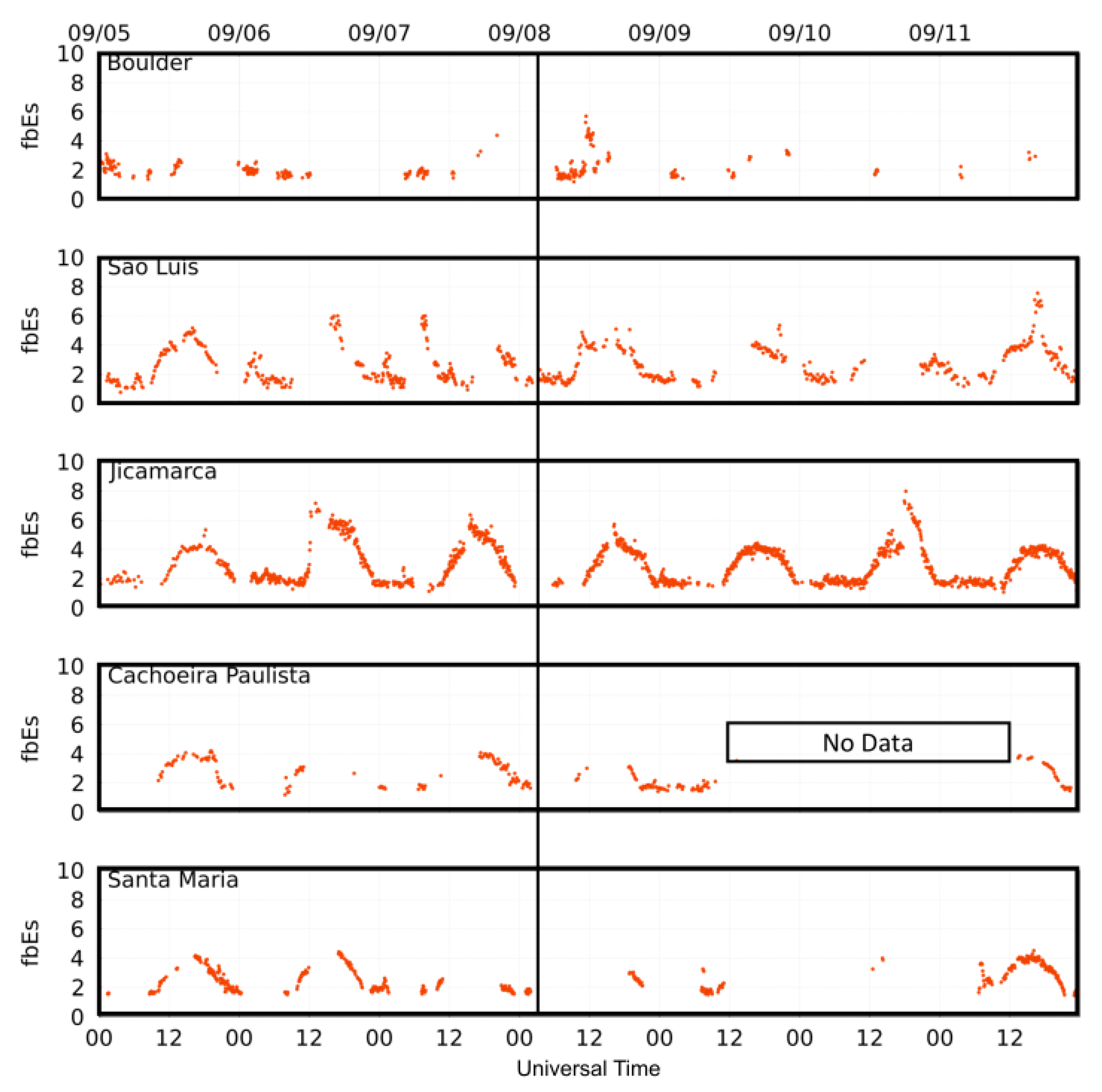
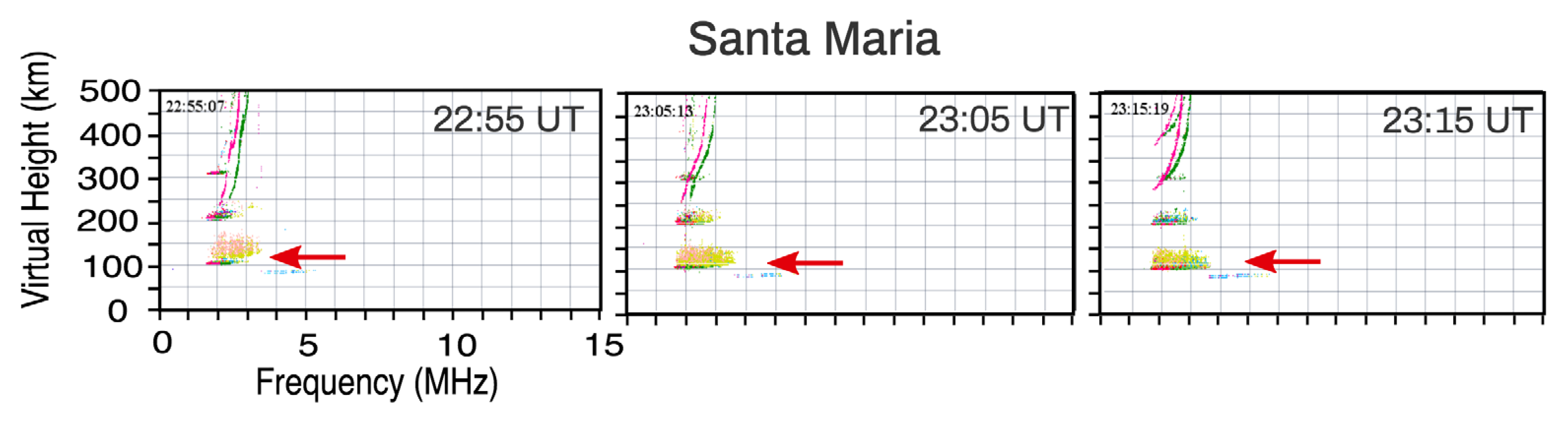
- In general, the Es layer development had no significant changes over Cachoeira Paulista and Santa Maria in the days that preceded and during the geomagnetic storms;
- (2)
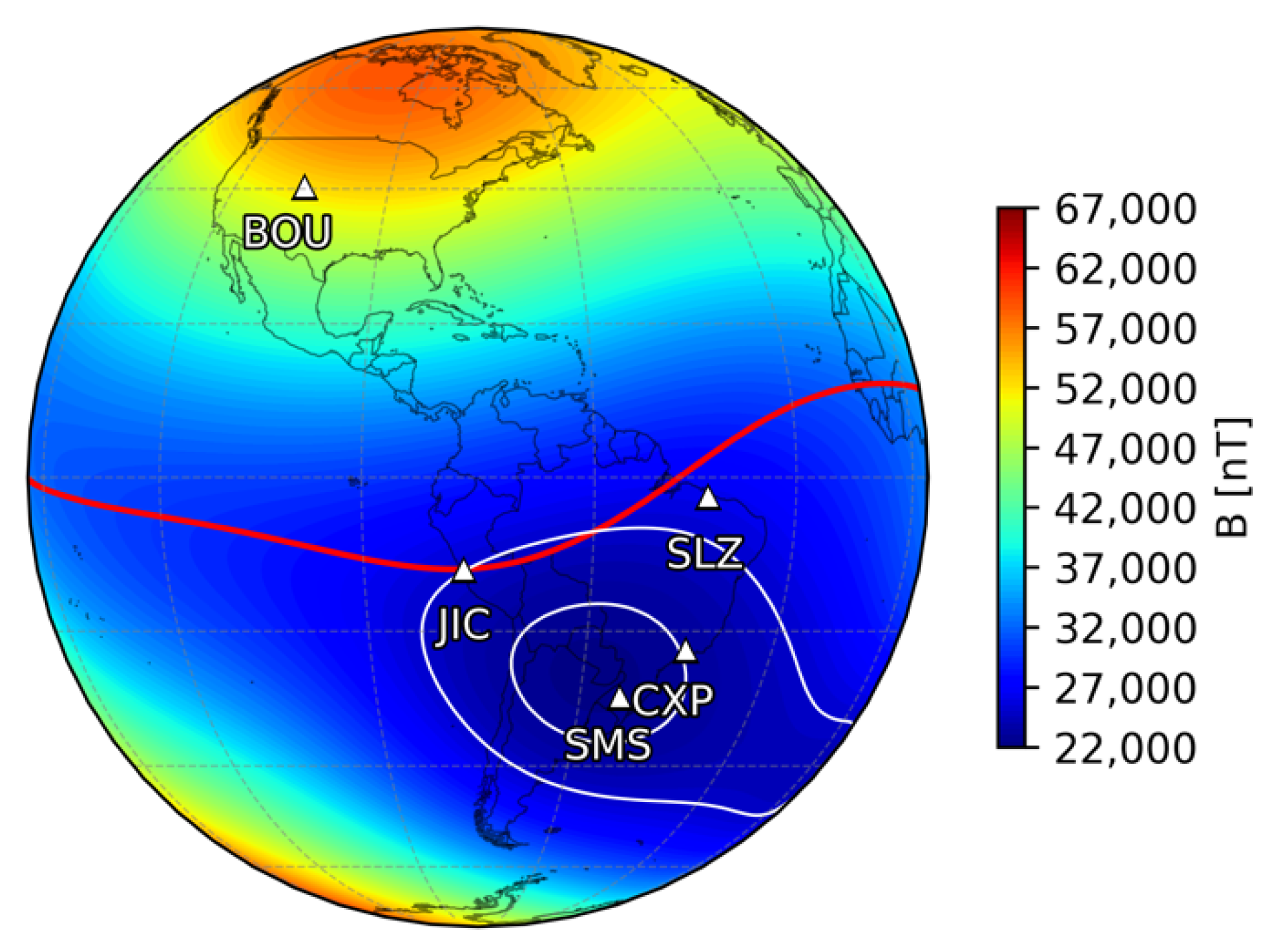
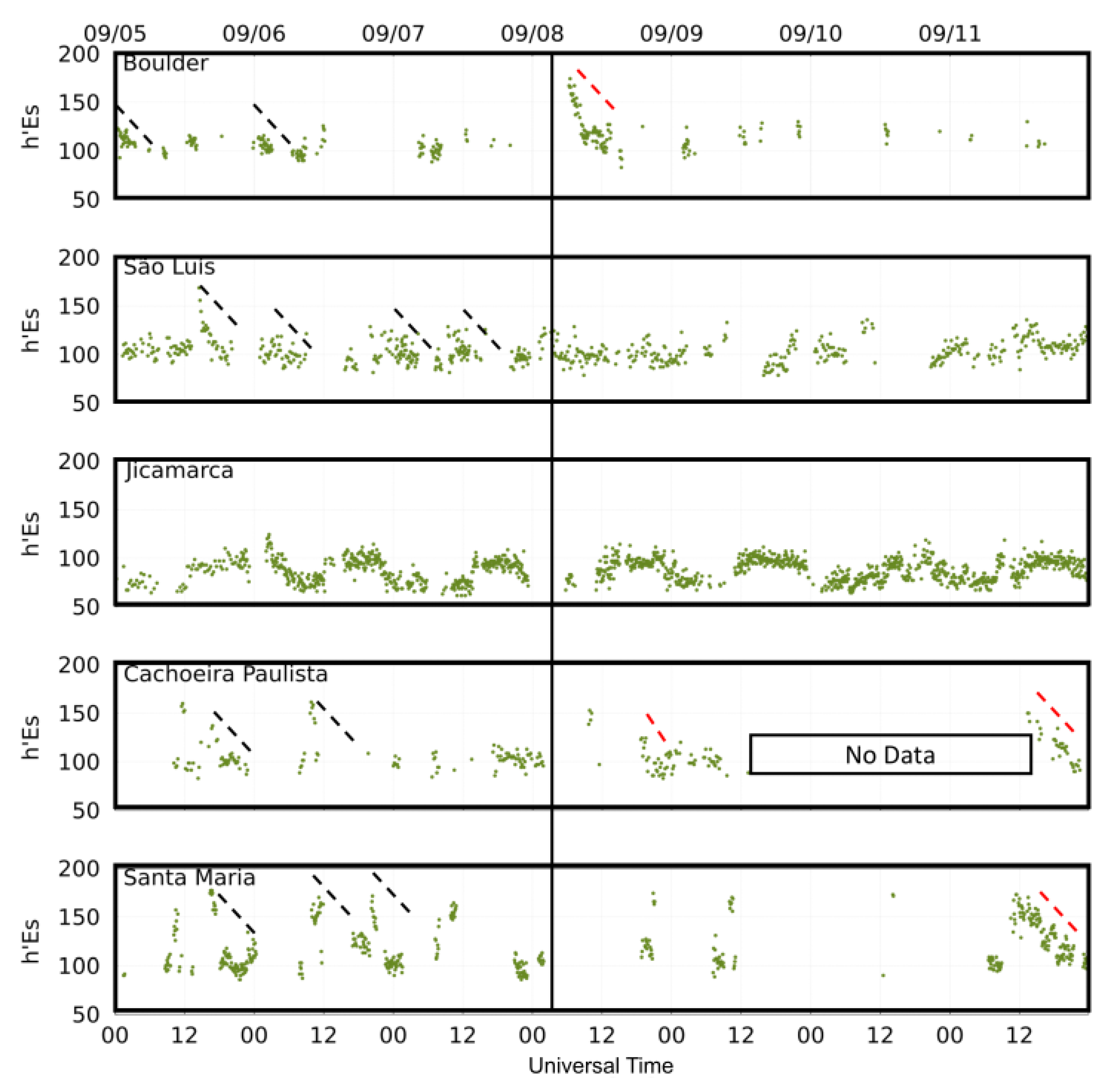
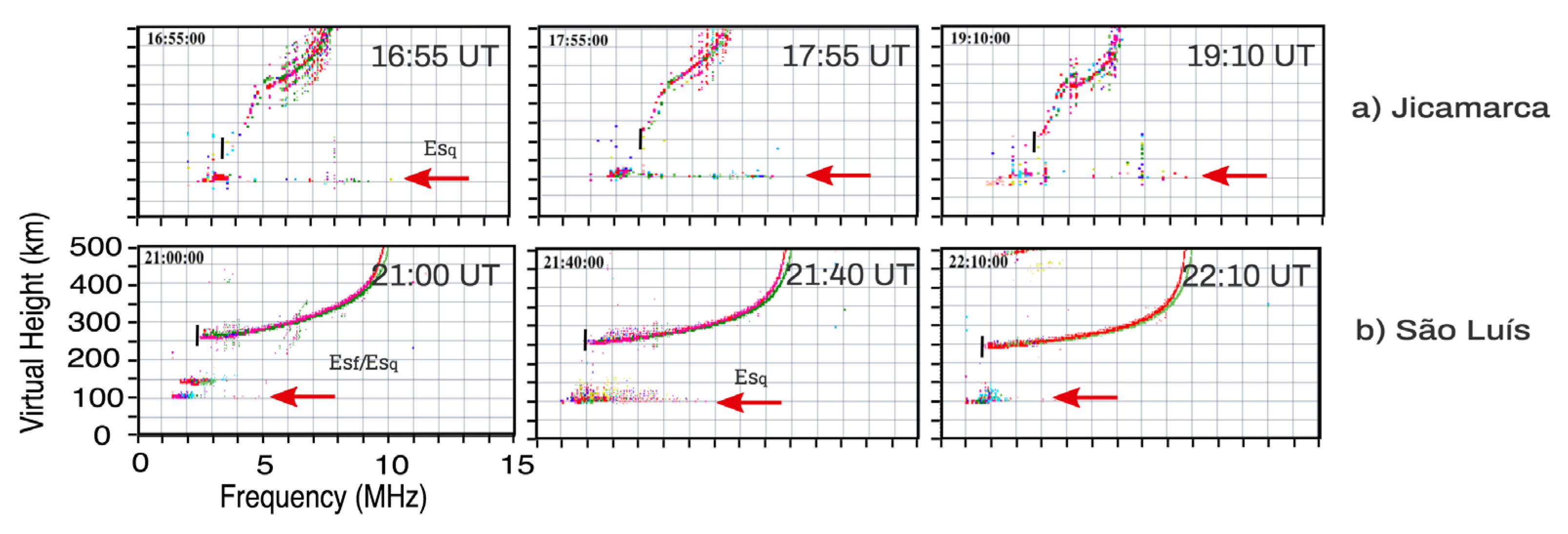
- In São Luís, we observed steady Es layers located around 100 km. This pattern is the same as the Es layer behavior over Jicamarca;
- (3)
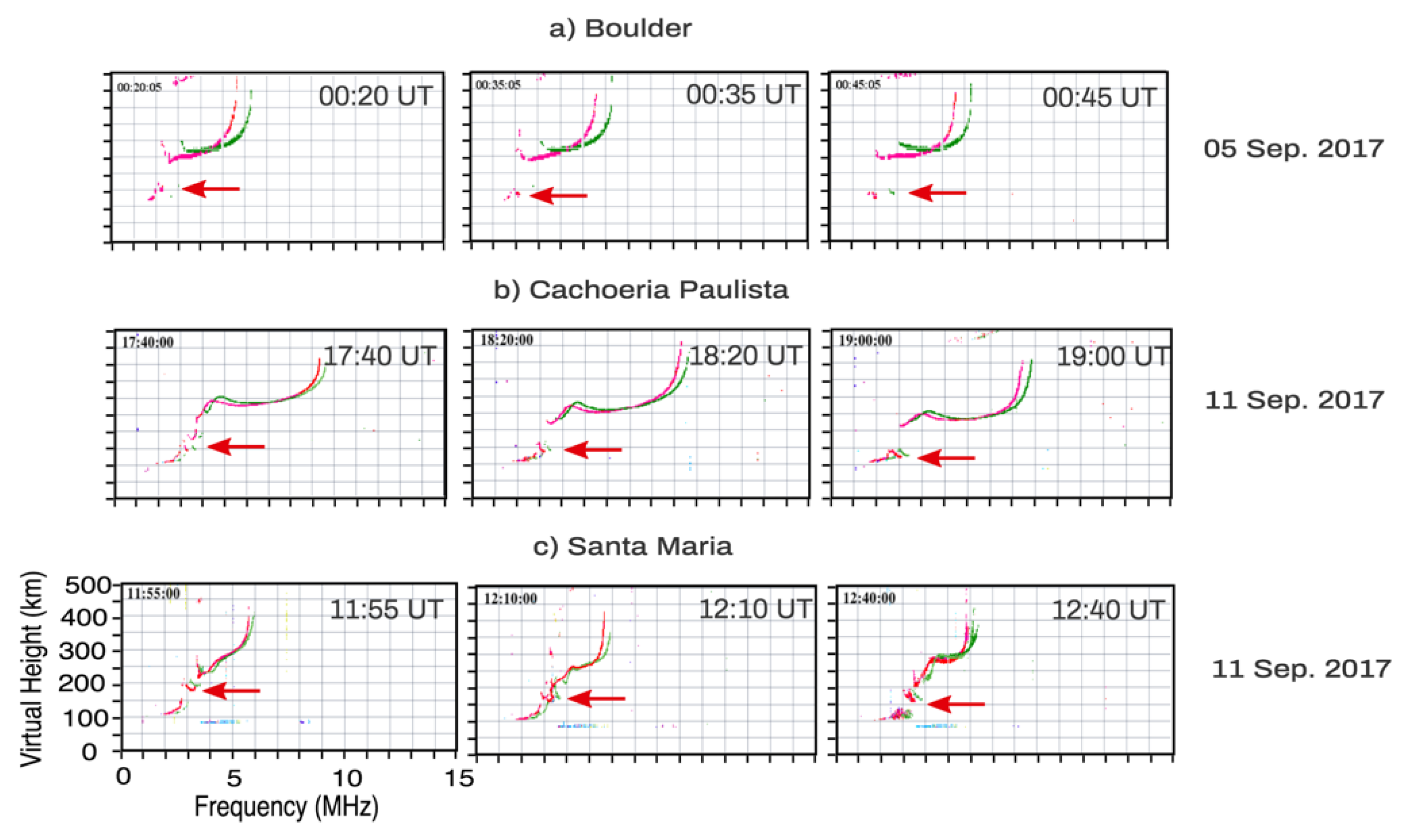
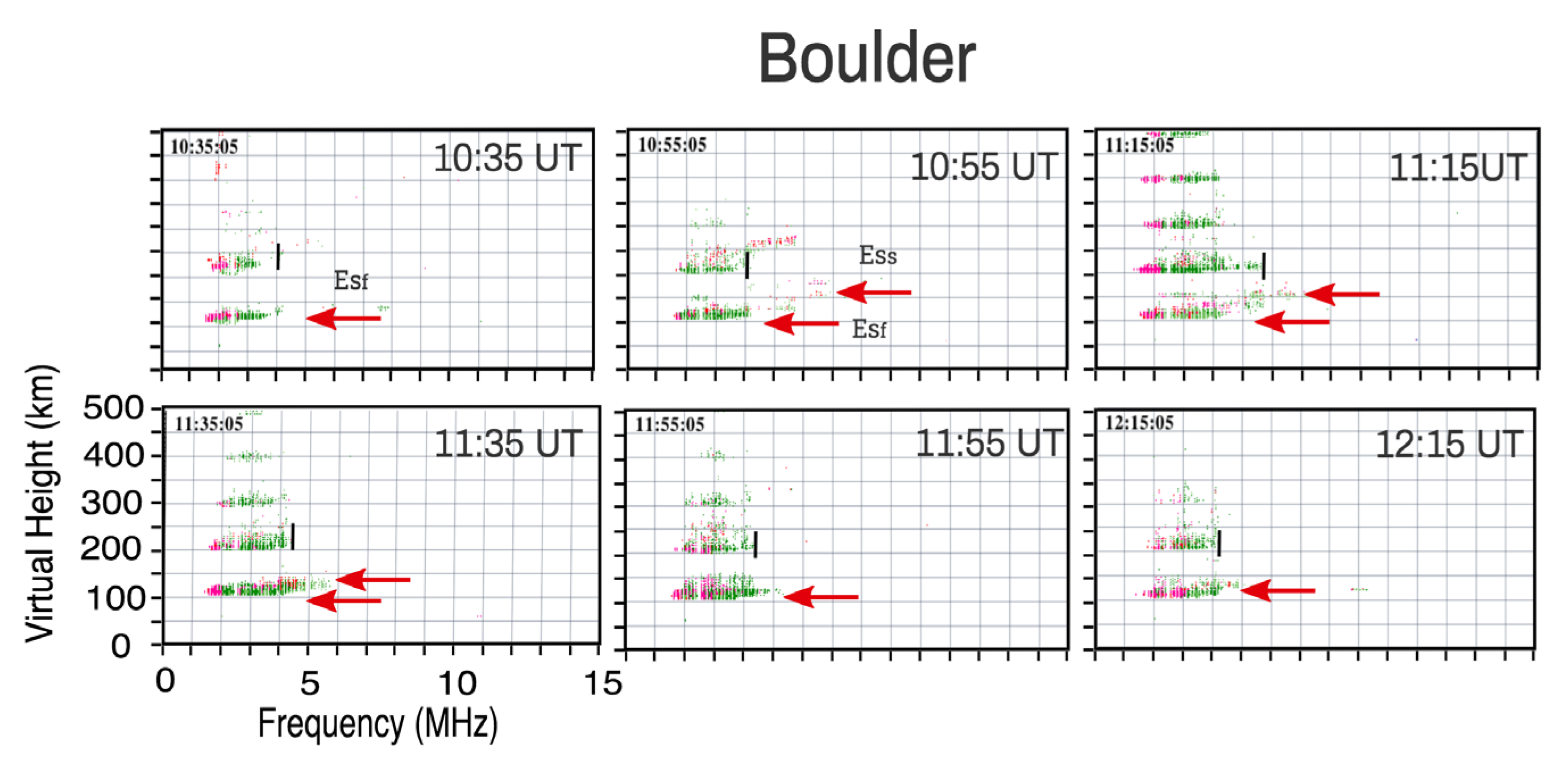
- The high Es layers occurred a few moments after the start of the magnetic storm over Boulder due to the presence of the “s” type (slant) (dashed red lines); and
- (4)
- The atypical spreading Es layer was observed over Boulder and Santa Maria.
4. Discussion
4.1. The Physical Dynamic in the Es Layer Development over the American Sector
4.2. The Gravity Wave Role in the Es Layer Development over Boulder during the Main Magnetic Storm Phase
5. Conclusions
Author Contributions
Funding
Institutional Review Board Statement
Informed Consent Statement
Data Availability Statement
Acknowledgments
Conflicts of Interest
References
- Haldoupis, C. A tutorial review on Sporadic E layers. Aeron. Earth’s Atmosph. Ionos. 2011, 29, 381–394. [Google Scholar]
- Resende, L.C.A.; Zhu, Y.; Denardini, C.; Batista, I.S.; Shi, J.; Moro, J.; Chen, S.S.; Conceição-Santos, F.; Da Silva, L.A.; Andrioli, V.F.; et al. New Findings of the Sporadic E (Es) Layer Development Around the Magnetic Equator During a High-Speed Solar (HSS) Wind Stream Event. J. Geophys. Res. 2021, 126, e2021JA029416. [Google Scholar] [CrossRef]
- Batista, I.S.; Abdu, M.A. Magnetic storm associated delayed sporadic E enhancements in the Brazilian Geomagnetic Anomaly. J. Geophys. Res. 1977, 82, 4777–4783. [Google Scholar] [CrossRef] [Green Version]
- Conceição-Santos, F.; Muella, M.T.A.H.; Resende, L.C.A.; Fagundes, P.R.; Andrioli, V.F.; Batista, P.P.; Carrasco, A.J. On the role of tidal winds in the descending of the high type of sporadic layer (Esh). Adv. Space Res. 2020, 65, 2131–2147. [Google Scholar] [CrossRef]
- Resende, L.C.A.; Denardini, C.M.; Batista, I.S. Abnormal fbEs enhancements in equatorial Es layers during magnetic storms of solar cycle 23. J. Atmos. Terr. Phys. 2013, 102, 228–234. [Google Scholar] [CrossRef]
- Resende, L.C.A.; Batista, I.S.; Denardini, C.M.; Carrasco, A.J.; Andrioli, V.F.; Moro, J.; Batista, P.P.; Chen, S.S. Competition between winds and electric fields in the formation of blanketing sporadic E layers at equatorial regions. Earth Space Sci. 2016, 68, 201. [Google Scholar] [CrossRef] [Green Version]
- Whitehead, J.D. Recent Work on Mid-Latitude and Equatorial Sporadic-E. J. Atmos. Terr. Phys. 1989, 51, 401–424. [Google Scholar] [CrossRef]
- Dagar, R.; Verma, P.; Napgal, O.; Setty, C.S.G.K. The relative effects of the electric fields and neutral winds on the formation of the equatorial sporadic layers. Ann. Geophys. 1977, 33, 333–340. [Google Scholar]
- Prasad, S.N.V.S.; Prasad, D.S.V.V.D.; Venkatesh, K.; Niranjan, K.; Rama Rao, P.V.S. Diurnal and seasonal variations in sporadic E-layer (Es layer) occurrences over equatorial, low and mid latitude stations—A comparative study. Indian J. Radio Space Phys. 2012, 41, 26–38. [Google Scholar]
- Resende, L.C.A.; Shi, J.; Denardini, C.M.; Batista, I.S.; Picanço, G.A.; Moro, J.; Chagas, R.A.J.; Barros, D.; Chen, S.S.; Nogueira, P.A.B.; et al. The Impact of the Disturbed Electric Field in the Sporadic E (Es) Layer Development Over Brazilian Region. J. Geophys. Res. 2021, 126, e2020JA028598. [Google Scholar] [CrossRef]
- Yamazaki, Y.; Richmond, A.; Maute, A.; Wu, Q.; Ortland, D.; Yoshikawa, A.; Adimula, I.; Rabiu, A.; Kunitake, M.; Tsugawa, T. Ground magnetic effects of the equatorial electrojet simulated by the TIE-GCM driven by TIMED satellite data. J. Geophys. Res. 2014, 118, 3150–3161. [Google Scholar] [CrossRef]
- Wang, J.; Zuo, X.; Sun, Y.-Y.; Yu, T.; Wang, Y.; Qiu, L.; Mao, T.; Yan, X.; Yang, N.; Yifan, Q.; et al. Multilayered sporadic-E response to the annular solar eclipse on June 21, 2020. Space Weather 2021, 19, e2020SW002643. [Google Scholar] [CrossRef]
- Manoj, C.S.M.; Maus, S.; Lühr, H.; Alken, P. Penetration characteristics of the interplanetary electric field to the daytime equatorial ionosphere. J. Geophys. Res. 2008, 113. [Google Scholar] [CrossRef]
- Zhang, K.; Wang, H.; Yamazaki, Y.; Xiong, C. Effects of Subauroral Polarization Streams on the Equatorial Electrojet During the Geomagnetic Storm on June 1, 2013. J. Geophys. Res. 2021, 126, e2021JA029681. [Google Scholar] [CrossRef]
- Ecklund, W.L.; Carter, D.A.; Balsley, B.B. Gradient drift irregularities in middle latitude sporadic E. J. Geophys. Res. 1981, 86, 8–862. [Google Scholar]
- Yan, C.; Chen, G.; Wang, Z.; Zhang, M.; Zhang, S.; Li, Y.; Huang, K.; Gong, W.; He, Z. Statistical characteristics of the low-latitude E-region irregularities observed by the HCOPAR in south China. J. Geophys. Res. 2021, 126, e2021JA029972. [Google Scholar] [CrossRef]
- Wakabayashi, M.; Ono, T. Multi-layer structure of mid-latitude sporadic-e observed during the SEEK-2 campaign. Ann. Geophys. 2005, 23, 2347–2355. [Google Scholar] [CrossRef] [Green Version]
- Reinisch, B.W.; Galkin, I.A.; Khmyrov, G.M.; Kozlov, A.V.; Bibl, K.; Lisysyan, I.A.; Cheney, G.P.; Huang, X.; Kitrosser, D.F.; Paznukhov, V.V.; et al. New Digisonde for research and monitoring applications. Rad. Sci. 2009, 44, 1 (RS0A24). [Google Scholar] [CrossRef]
- Reddy, C.A.; Rao, M. On the physical significance of the Es parameters ƒbEs, ƒEs, and ƒoEs. J. Geophys. Res. 1968, 73, 215–224. [Google Scholar] [CrossRef]
- Resende, L.C.A.; Batista, I.S.; Denardini, C.M.; Batista, P.P.; Carrasco, A.J.; Andrioli, V.F.; Moro, J. Simulations of blanketing sporadic E-layer over the Brazilian sector driven by tidal winds. J. Atmos. Terr. Phys. 2017, 154, 104–114. [Google Scholar] [CrossRef]
- Resende, L.C.A.; Batista, I.S.; Denardini, C.M.; Batista, P.P.; Carrasco, A.J.; Andrioli, V.F.; Moro, J. The influence of tidal winds in the formation of blanketing sporadic E-layer over equatorial Brazilian region. J. Atmos. Terr. Phys. 2017, 171, 64–67. [Google Scholar] [CrossRef]
- Carrasco, A.J.; Batista, I.S.; Abdu, M.A. Simulation of the sporadic E layer response to pre-reversal associated evening vertical electric field enhancement near dip equator. J. Geophys. Res. 2007, 112, 324–335. [Google Scholar]
- Hagan, M.E.; Forbes, J.M. Migrating and nonmigrating diurnal tides in the middle and upper atmosphere excited by tropospheric latent heat release. J. Geophys. Res. 2002, 107, 4754. [Google Scholar] [CrossRef]
- Hagan, M.E.; Forbes, J.M. Migrating and nonmigrating semidiurnal tides in the upper atmosphere excited by tropospheric latent heat release. J. Geophys. Res. 2003, 108, 1062. [Google Scholar] [CrossRef]
- Wickert, J.; Michalak, G.; Schmidt, T.; Beyerle, G.; Cheng, C.Z.; Healy, S.B.; Heise, S.; Huang, C.Y.; Jakowski, N.; Kohler, W.; et al. GPS radio occultation: Results from CHAMP, GRACE and FORMOSAT-3/COSMIC. Terr. Atmos. Ocean. Sci. 2009, 20, 35–50. [Google Scholar] [CrossRef]
- Arras, C.; Jacobi, C.; Wickert, J. Semidiurnal tidal signature in sporadic E occurrence rates derived from GPS radio occultation measurements at higher midlatitudes. Ann. Geophys. 2009, 27, 2555–2563. [Google Scholar] [CrossRef] [Green Version]
- Wu, D.L.; Ao, C.O.; Hajj, G.A.; de la Torre Juarez, M.; Mannucci, A.J. Sporadic E morphology from GPS CHAMP radio occultation. J. Geophys. Res. 2005, 110, A01306. [Google Scholar]
- Arras, C.; Wickert, J. Estimation of ionospheric sporadic E intensities from GPS radio occultation measurements. J. Atmos. Terr. Phys. 2017, 171, 60–63. [Google Scholar] [CrossRef]
- Stone, E.C.; Frandsen, A.M.; Mewaldt, R.A.; Christian, E.R.; Margolies, D.; Ormes, J.F.; Snow, F. The advanced Composition Explorer. Spa Sci. Rev. 1998, 86, 1–22. [Google Scholar] [CrossRef]
- Gonzalez, W.D.; Joselyn, J.A.; Kamide, Y.; Kroehl, H.W.; Rostoker, G.; Tsurutani, B.T.; Vasyliunas, V.M. What is a magnetic storm? J. Geophys. Res. 1994, 99 (A4), 5771–5792. [Google Scholar] [CrossRef] [Green Version]
- Guyer, S.; Can, Z. Solar Flare Effects on the Ionosphere. In Proceedings of the 2013 6th International Conference on Recent Advances in Space Technologies (RAST), Istanbul, Turkey, 12–14 June 2013; pp. 729–733. [Google Scholar]
- Tsurutani, B.T.; Verkhoglyadova, O.P.; Mannucci, A.J.; Lakhina, G.S.; Li, G.; Zank, G.P. A brief review of ‘‘solar flare effects’’ on the ionosphere. Radio Sci. 2009, 44, RS0A17. [Google Scholar] [CrossRef]
- Sahai, Y.; Becker-Guedes, F.; Fagundes, P.R.; Lima, W.L.C.; de Abreu, A.J.; Guarnieri, F.L.; Candido, C.M.N.; Pillat, V.G. Unusual ionospheric effects observed during the intense 28 October 2003 solar flare in the Brazilian sector. Ann. Geophys. 2006, 25, 2497. [Google Scholar] [CrossRef]
- Denardini, C.M.; Resende, L.C.A.; Moro, J.; Chen, S.S. Occurrence of the blanketing sporadic E layer during the recovery phase of the October 2003 superstorm. Earth Space Sci. 2016, 68, 80. [Google Scholar] [CrossRef] [Green Version]
- Santos, A.M.; Batista, I.S.; Abdu, M.A.; Sobral, J.H.; Souza, J.R.; Brum, C.G.M. Climatology of intermediate descending layers (or 150 km echoes) over the equatorial and low-latitude regions of Brazil during the deep solar minimum of 2009. Ann. Geophys. 2020, 37, 1005–1024. [Google Scholar] [CrossRef] [Green Version]
- Conceição-Santos, F.; Muella, M.T.A.H.; Resende, L.C.A.; Fagundes, P.R.; Andrioli, V.F.; Batista, P.P. Occurrence and Modeling Examination of Sporadic-E Layers in the Region of the South America (Atlantic) Magnetic Anomaly. J. Geophys. Res. 2019, 124, 9676–9694. [Google Scholar] [CrossRef]
- Jacobi, C.; Arras, C.; Geißler, C.; Lilienthal, F. Quarterdiurnal signature in sporadic E occurrence rates and comparison with neutral wind shear. Ann. Geophys. 2019, 37, 273–288. [Google Scholar] [CrossRef]
- Resende, L.C.A.; Shi, J.; Denardini, C.M.; Batista, I.S.; Nogueira, P.A.B.; Arras, C.; Andrioli, V.F.; Moro, J.; Da Silva, L.A.; Carrasco, A.J.; et al. The influence of disturbance dynamo electric field in the formation of strong sporadic E layers over Boa Vista, a low-latitude station in the American sector. J. Geophys. Res. 2020, 125, e2019JA027519. [Google Scholar] [CrossRef]
- Moro, J.; Xu, J.; Denardini, C.M.; Resende, L.C.A.; Da Silva, L.A.; Chen, S.S.; Carrasco, A.J.; Liu, Z.; Wang, C.; Schuch, N.J. Different Sporadic-E (Es) Layer Types Development During the August 2018 Geomagnetic Storm: Evidence of Auroral Type (Esa) over the SAMA Region. J. Geophys. Res. 2020, 127, e2021JA029701. [Google Scholar] [CrossRef]
- Piggott, W.; Rawer, K. Handbook of Ionogram Interpretation and Reduction; US Department of Commerce, Ed.; National Academy of Sciences: Washington, DC, USA, 1972; p. 352. [Google Scholar]
- Batista, I.S.; Diogo, E.M.; Souza, J.R.; Abdu, M.A.; Bailey, G.J. Equatorial Ionization Anomaly: The Role of Thermospheric Winds and the Effects of the Geomagnetic Field Secular Variation. In Aeronomy of the Earth’s Atmosphere and Ionosphere; Springer: Dordrecht, The Netherlands, 2011; pp. 317–328. [Google Scholar]
- Abdu, M.A.; Batista, I.S.; MacDougall, J.; Sobral, J.H.A.; Muralikrishna, P. Permanent changes in sporadic E layers over Fortaleza, Brazil. Adv. Spa. Res. 1997, 20, 2165–2168. [Google Scholar] [CrossRef] [Green Version]
- Bulusu, J.; Archana, R.; Arora, K.; Nelapatla, P.; Nagarajan, N. Effect of Disturbance Electric Fields on Equatorial Electrojet Over Indian Longitudes: Ionospheric Disturbance Electric Field. J. Geophys. Res. 2018, 123, 5894–5916. [Google Scholar] [CrossRef]
- Wang, H.; Hermann, L.; Zheng, Z.; Kedeng, Z. Dependence of the Equatorial Electrojet on Auroral Activity and In Situ Solar Insulation. J. Geophys. Res. 2019, 124, 10659–10673. [Google Scholar] [CrossRef]
- Cohen, R.; Calvert, W.; Bowles, K.L. On nature of equatorial slant sporadic E. J. Geophys. Res. 1962, 67, 965–975. [Google Scholar] [CrossRef]
- Didebulidze, G.G.; Dalakishvili, G.; Todua, M. Formation of Multilayered Sporadic E under an Influence of Atmospheric Gravity Waves (AGWs). Atmosphere 2020, 11, 653–675. [Google Scholar] [CrossRef]
- Fritts, D.C.; Alexander, J. Gravity wave dynamics and effects in the middle atmosphere, Rev. Geoph. 2003, 41, 1–68. [Google Scholar]


Publisher’s Note: MDPI stays neutral with regard to jurisdictional claims in published maps and institutional affiliations. |
© 2022 by the authors. Licensee MDPI, Basel, Switzerland. This article is an open access article distributed under the terms and conditions of the Creative Commons Attribution (CC BY) license (https://creativecommons.org/licenses/by/4.0/).
Share and Cite
Resende, L.C.A.; Zhu, Y.; Arras, C.; Denardini, C.M.; Chen, S.S.; Moro, J.; Barros, D.; Chagas, R.A.J.; Da Silva, L.A.; Andrioli, V.F.; et al. Analysis of the Sporadic-E Layer Behavior in Different American Stations during the Days around the September 2017 Geomagnetic Storm. Atmosphere 2022, 13, 1714. https://doi.org/10.3390/atmos13101714
Resende LCA, Zhu Y, Arras C, Denardini CM, Chen SS, Moro J, Barros D, Chagas RAJ, Da Silva LA, Andrioli VF, et al. Analysis of the Sporadic-E Layer Behavior in Different American Stations during the Days around the September 2017 Geomagnetic Storm. Atmosphere. 2022; 13(10):1714. https://doi.org/10.3390/atmos13101714
Chicago/Turabian StyleResende, Laysa C. A., Yajun Zhu, Christina Arras, Clezio M. Denardini, Sony S. Chen, Juliano Moro, Diego Barros, Ronan A. J. Chagas, Lígia A. Da Silva, Vânia F. Andrioli, and et al. 2022. "Analysis of the Sporadic-E Layer Behavior in Different American Stations during the Days around the September 2017 Geomagnetic Storm" Atmosphere 13, no. 10: 1714. https://doi.org/10.3390/atmos13101714