
Development and Application of the SmartAQ High-Resolution Air Quality and Source Apportionment Forecasting System for European Urban Areas

 ,
,  ,
, 
Abstract
:1. Introduction
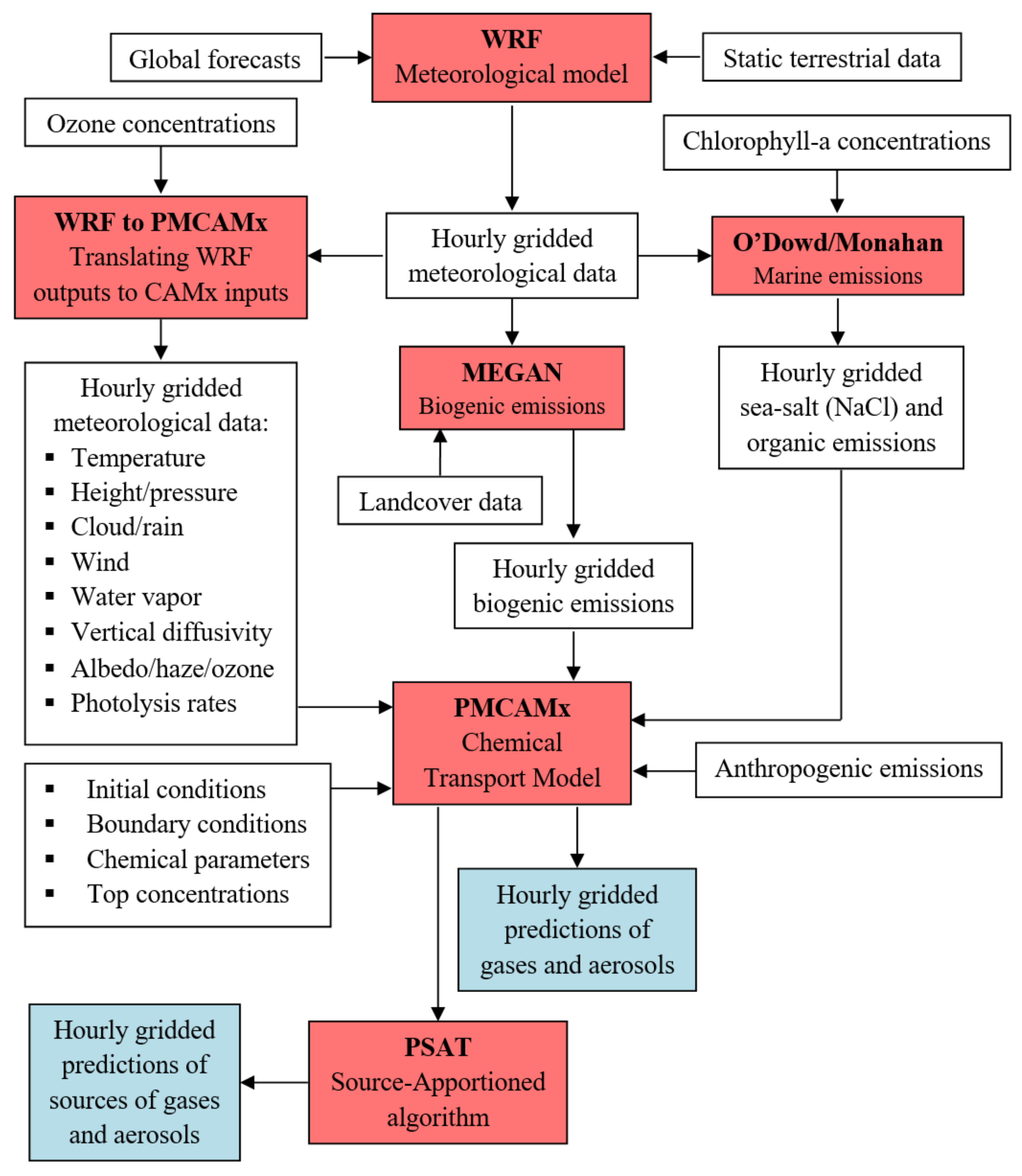
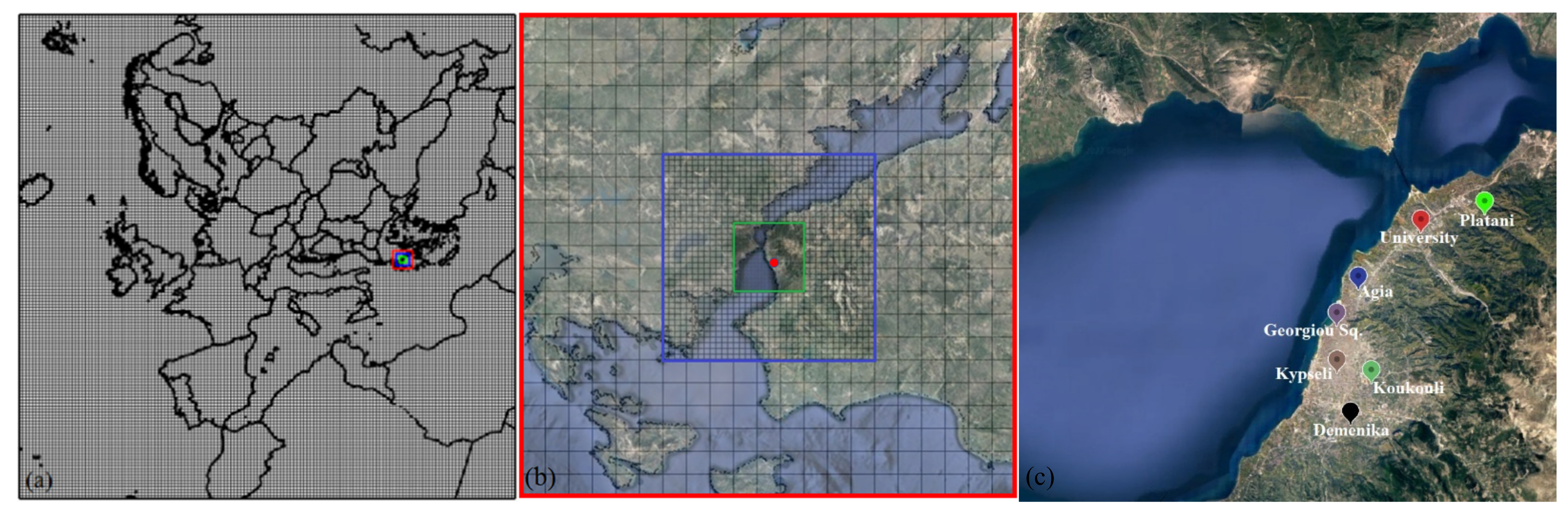
2. SmartAQ System
2.1. Meteorology
2.2. Air Quality Model
2.3. Biogenic Emissions
2.4. Marine Aerosol Emissions
2.5. Anthropogenic Emissions
2.5.1. Emissions for the European Domain
2.5.2. Emissions for the Urban Domain of Patras
2.6. Source Apportionment Algorithm
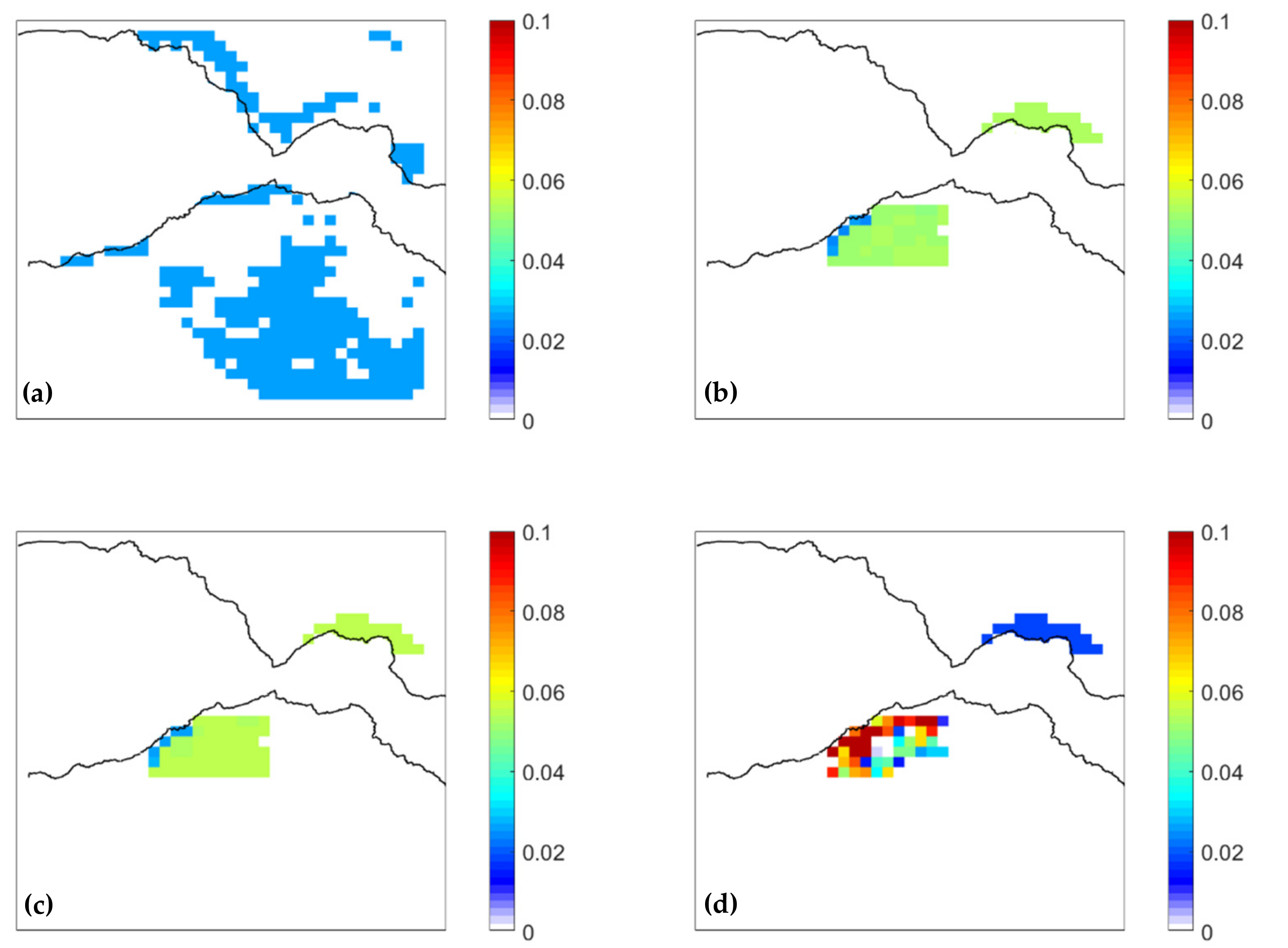
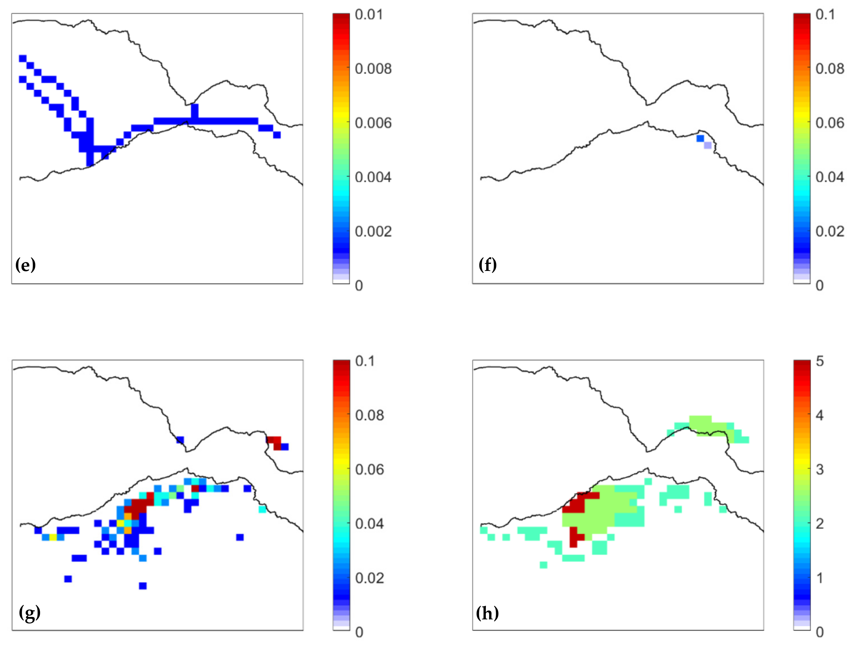
3. Results
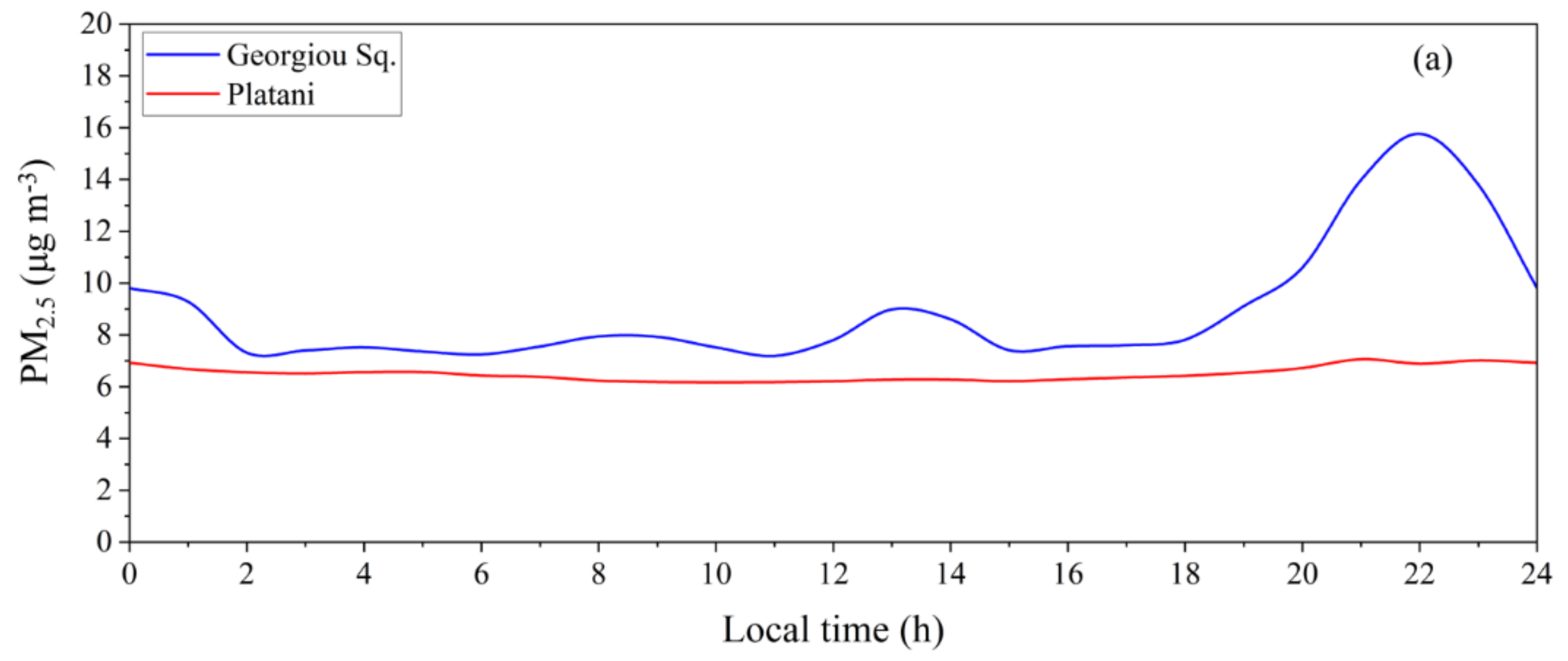
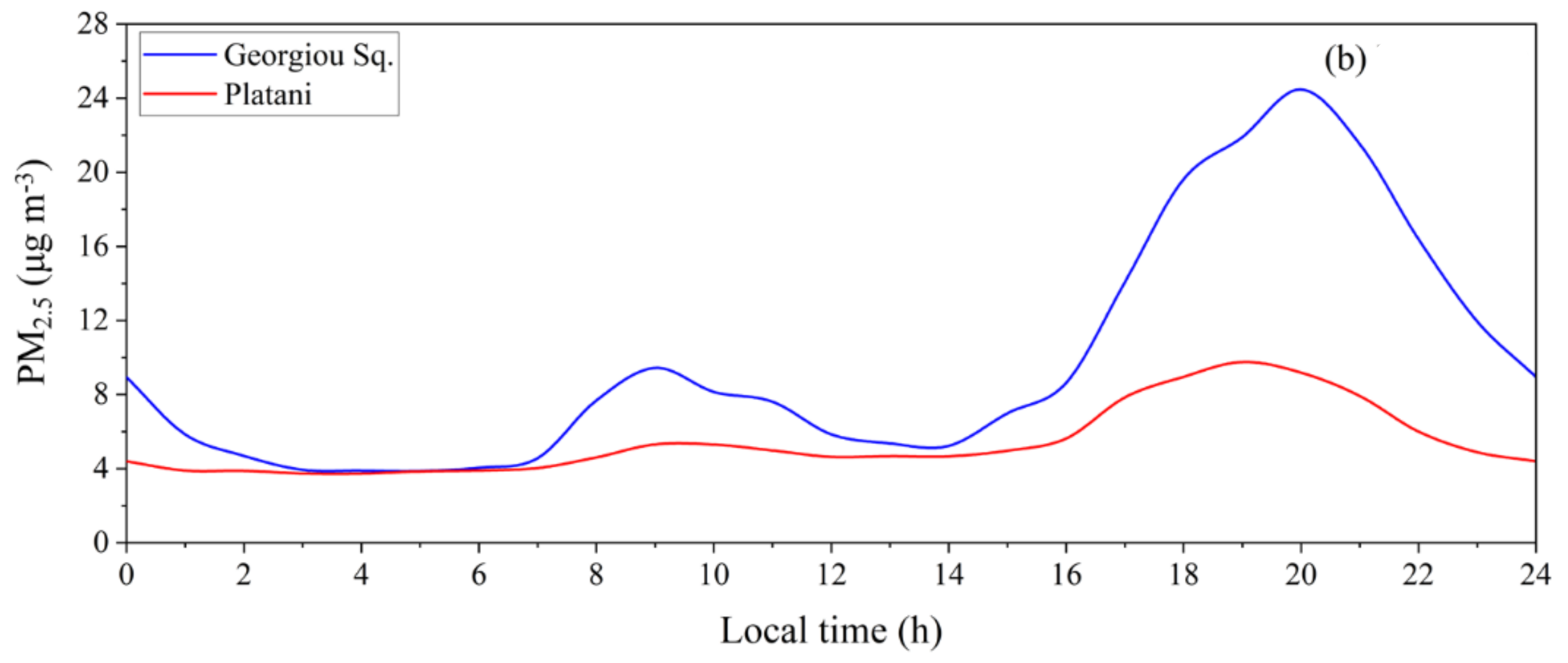
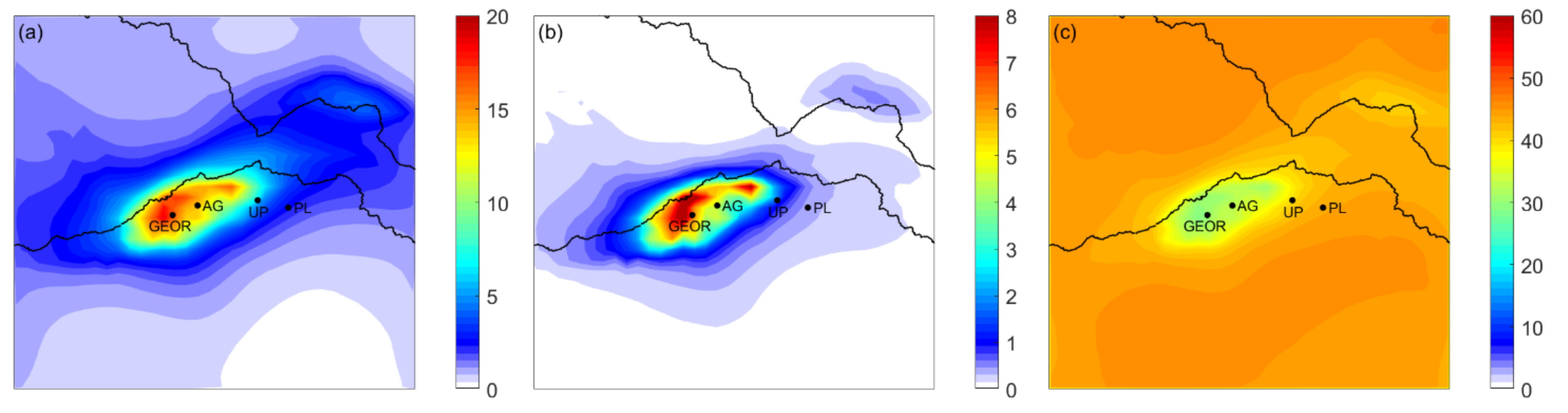
3.1. PM2.5 Predictions
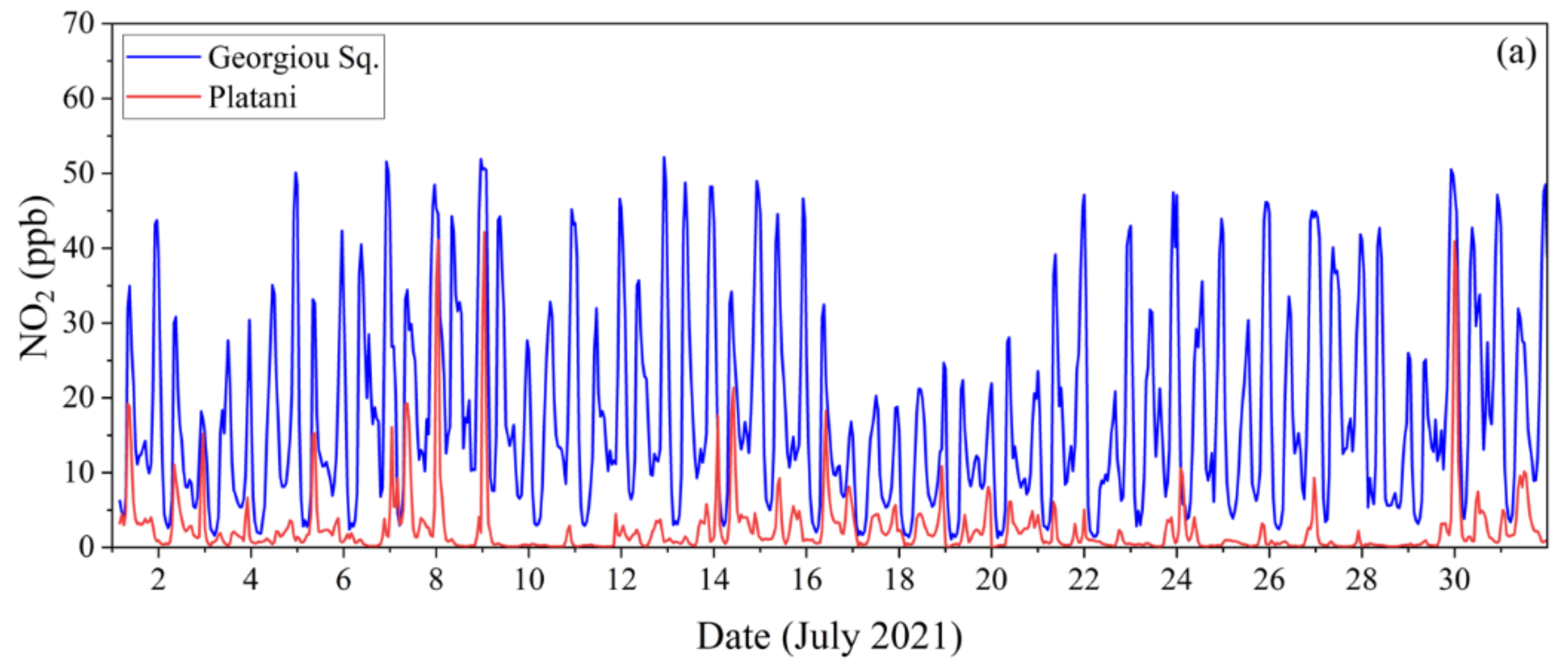
3.2. Predictions for Gas-Phase Pollutants
4. Discussion
5. Conclusions
Supplementary Materials
Author Contributions
Funding
Institutional Review Board Statement
Informed Consent Statement
Data Availability Statement
Conflicts of Interest
References
- Brugha, R.; Grigg, J. Urban air pollution and respiratory infections. Paediatr. Respir. Rev. 2014, 15, 194–199. [Google Scholar] [CrossRef] [PubMed]
- Du, Y.; Xu, X.; Chu, M.; Guo, Y.; Wang, J. Air particulate matter and cardiovascular disease: The epidemiological, biomedical and clinical evidence. J. Thorac. Dis. 2016, 8, 8–19. [Google Scholar]
- World Health Organization (WHO). Fact Sheet: Ambient (Outdoor) Air Pollution. 2021. Available online: https://www.who.int/news-room/fact-sheets/detail/ambient-(outdoor)-air-quality-and-health/ (accessed on 3 September 2022).
- Boningari, T.; Smirniotis, P.G. Impact of nitrogen oxides on the environment and human health: Mn-based materials for the NOx abatement. Curr. Opin. Chem. Eng. 2016, 13, 133–141. [Google Scholar] [CrossRef]
- Kukkonen, J.; Olsson, T.; Schultz, D.M.; Baklanov, A.; Klein, T.; Miranda, A.I.; Monteiro, A.; Hirtl, M.; Tarvainen, V.; Boy, M.; et al. A review of operational, regional-scale, chemical weather forecasting models in Europe. Atmos. Chem. Phys. 2012, 12, 1–87. [Google Scholar]
- Kaya, K.; Öğüdücü, S.G. Deep Flexible Sequential (DFS) model for air pollution forecasting. Sci. Rep. 2020, 10, 3346. [Google Scholar] [CrossRef] [Green Version]
- Delle Monache, L.; Alessandrini, S.; Djalalova, I.; Wilczak, J.; Knievel, J.C.; Kumar, R. Improving air quality predictions over the United States with an analog ensemble. Weather Forecast. 2020, 35, 2145–2162. [Google Scholar] [CrossRef] [Green Version]
- Hamill, T.M.; Whitaker, J.S. Probabilistic quantitative precipitation forecasts based on reforecast analogs: Theory and application. Mon. Weather Rev. 2006, 134, 3209–3229. [Google Scholar] [CrossRef]
- Pappa, A.; Kioutsioukis, I. Forecasting particulate pollution in an urban area: From Copernicus to sub-km scale. Atmosphere 2021, 12, 881. [Google Scholar] [CrossRef]
- Zhang, Y.; Bocquet, M.; Mallet, V.; Seigneur, C.; Baklanov, A. Real-time air quality forecasting, part I: History, techniques, and current status. Atmos. Environ. 2012, 60, 632–655. [Google Scholar] [CrossRef]
- Marécal, V.; Peuch, V.-H.; Andersson, C.; Andersson, S.; Arteta, J.; Beekmann, M.; Benedictow, A.; Bergström, R.; Bessagnet, B.; Cansado, A.; et al. A regional air quality forecasting system over Europe: The MACC-II daily ensemble production. Geosci. Model Dev. 2015, 8, 2777–2813. [Google Scholar] [CrossRef] [Green Version]
- CAMS. Regional Production, Updated Documentation Covering All Regional Operational Systems and the ENSEMBLE. ECMWF Copernicus Report. 2020. Available online: https://atmosphere.copernicus.eu/sites/default/files/2020-09/CAMS50_2018SC2_D2.0.2-U2_Models_documentation_202003_v2.pdf (accessed on 3 September 2022).
- Rouil, L.; Honoré, C.; Vautard, R.; Beekmann, M.; Bessagnet, B.; Malherbe, L.; Meleux, F.; Dufour, A.; Elichegaray, C.; Flaud, J.M.; et al. PREV’AIR: An operational forecasting and mapping system for air quality in Europe. Bull. Am. Meteorol. Soc. 2009, 90, 73–83. [Google Scholar] [CrossRef] [Green Version]
- Lee, K.; Yu, J.; Lee, S.; Park, M.; Hong, H.; Park, S.Y.; Choi, M.; Kim, J.; Kim, Y.; Woo, J.-H.; et al. Development of Korean Air Quality Prediction System version 1 (KAQPS v1) with focuses on practical issues. Geosci. Model Dev. 2020, 13, 1055–1073. [Google Scholar] [CrossRef]
- Brasseur, G.P.; Xie, Y.; Petersen, A.K.; Bouarar, I.; Flemming, J.; Gauss, M.; Jiang, F.; Kouznetsov, R.; Kranenburg, R.; Mijling, B.; et al. Ensemble forecasts of air quality in eastern China–Part 1: Model description and implementation of the MarcoPolo-Panda prediction system, version 1. Geosci. Model Dev. 2019, 12, 33–67. [Google Scholar] [CrossRef] [Green Version]
- Katragkou, E.; Kioutsioukis, I.; Poupkou, A.; Lisaridis, I.; Markakis, K.; Karathanasis, S.; Melas, D.; Balis, D. An air quality study for Greece with the MM5/CAMx modelling system. In Proceedings of the Electronic ‘Envisat Symposium 2007′, Montreux, Switzerland, 23–27 April 2007. [Google Scholar]
- Donahue, N.M.; Robinson, A.L.; Stanier, C.O.; Pandis, S.N. Coupled partitioning, dilution, and chemical aging of semivolatile organics. Environ. Sci. Technol. 2006, 40, 2635–2643. [Google Scholar] [CrossRef]
- Robinson, A.L.; Donahue, N.M.; Shrivastava, M.K.; Weitkamp, E.A.; Sage, A.M.; Grieshop, A.P.; Lane, T.E.; Pierce, J.R.; Pandis, S.N. Rethinking organic aerosols: Semivolatile emissions and photochemical aging. Science 2007, 315, 1259–1262. [Google Scholar] [CrossRef]
- Murphy, B.N.; Donahue, N.M.; Robinson, A.L.; Pandis, S.N. A naming convention for atmospheric organic aerosol. Atmos. Chem. Phys. 2014, 14, 5825–5839. [Google Scholar] [CrossRef] [Green Version]
- Bergström, R.; Denier van der Gon, H.A.C.; Prévôt, A.S.H.; Yttri, K.E.; Simpson, D. Modelling of organic aerosols over Europe (2002–2007) using a volatility basis set (VBS) framework: Application of different assumptions regarding the formation of secondary organic aerosol. Atmos. Chem. Phys. 2012, 12, 8499–8527. [Google Scholar] [CrossRef] [Green Version]
- Li, Y.P.; Elbern, H.; Lu, K.D.; Friese, E.; Kiendler-Scharr, A.; Mentel, T.F.; Wang, X.S.; Wahner, A.; Zhang, Y.H. Updated aerosol module and its application to simulate secondary organic aerosols during IMPACT campaign May 2008. Atmos. Chem. Phys. 2013, 13, 6289–6304. [Google Scholar] [CrossRef] [Green Version]
- Simpson, D.; Benedictow, A.; Berge, H.; Bergström, R.; Emberson, L.D.; Fagerli, H.; Flechard, C.R.; Hayman, G.D.; Gauss, M.; Jonson, J.E.; et al. The EMEP MSC-W chemical transport model–technical description. Atmos. Chem. Phys. 2012, 12, 7825–7865. [Google Scholar] [CrossRef] [Green Version]
- Hodzic, A.; Kasibhatla, P.S.; Jo, D.S.; Cappa, C.D.; Jimenez, J.L.; Madronich, S.; Park, R.J. Rethinking the global secondary organic aerosol (SOA) budget: Stronger production, faster removal, shorter lifetime. Atmos. Chem. Phys. 2016, 16, 7917–7941. [Google Scholar] [CrossRef] [Green Version]
- Honoré, C.; Rouil, L.; Vautard, R.; Beekmann, M.; Bessagnet, B.; Dufour, A.; Elichegaray, C.; Flaud, J.-M.; Malherbe, L.; Meleux, F.; et al. Predictability of European air quality: Assessment of 3 years of operational forecasts and analyses by the PREV’AIR system. J. Geophys. Res. 2008, 113, D04301. [Google Scholar] [CrossRef]
- Woo, J.-H.; Choi, K.-C.; Kim, H.K.; Baek, B.H.; Jang, M.; Eum, J.-H.; Song, C.H.; Ma, Y.-I.; Sunwoo, Y.; Chang, L.-S.; et al. Development of an anthropogenic emissions processing system for Asia using SMOKE. Atmos. Environ. 2012, 58, 5–13. [Google Scholar] [CrossRef]
- Allan, J.D.; Williams, P.I.; Morgan, W.T.; Martin, C.L.; Flynn, M.J.; Lee, J.; Nemitz, E.; Phillips, G.J.; Gallagher, M.W.; Coe, H. Contributions from transports solid fuel burning, and cooking to primary organic aerosols in two UK cities. Atmos. Chem. Phys. 2010, 10, 647–668. [Google Scholar] [CrossRef] [Green Version]
- Mohr, C.; DeCarlo, P.F.; Heringa, M.F.; Chirico, R.; Slowik, J.G.; Richter, R.; Reche, C.; Alastuey, A.; Querol, X.; Seco, R.; et al. Identification and quantification of organic aerosol from cooking and other sources in Barcelona using aerosol mass spectrometer data. Atmos. Chem. Phys. 2012, 12, 1649–1665. [Google Scholar] [CrossRef] [Green Version]
- Crippa, M.; DeCarlo, P.F.; Slowik, J.G.; Mohr, C.; Heringa, M.F.; Chirico, R.; Poulain, L.; Freutel, F.; Sciare, J.; Cozic, J.; et al. Wintertime aerosol chemical composition and source apportionment of the organic fraction in the metropolitan area of Paris. Atmos. Chem. Phys. 2013, 13, 961–981. [Google Scholar] [CrossRef] [Green Version]
- Kostenidou, E.; Florou, K.; Kaltsonoudis, C.; Tsiflikiotou, M.; Vratolis, E.; Eleftheriadis, K.; Pandis, S.N. Sources and chemical characterization of organic aerosol during the summer in the eastern Mediterranean. Atmos. Chem. Phys. 2015, 15, 11355–11371. [Google Scholar] [CrossRef] [Green Version]
- Florou, K.; Papanastasiou, D.K.; Pikridas, M.; Kaltsonoudis, C.; Louvaris, E.; Gkatzelis, G.I.; Patoulias, D.; Mihalopoulos, N.; Pandis, S.N. The contribution of wood burning and other pollution sources to wintertime organic aerosol levels in two Greek cities. Atmos. Chem. Phys. 2017, 17, 3145–3163. [Google Scholar] [CrossRef] [Green Version]
- Skamarock, W.C.; Klemp, J.B.; Dudhia, J.; Gill, D.O.; Liu, Z.; Berner, J.; Wang, W.; Powers, J.G.; Duda, M.G.; Barker, D.M.; et al. A description of the Advanced Research WRF Model Version 4.1; No. NCAR/TN-556+STR; National Center for Atmospheric Research: Boulder, CO, USA, 20 July 2021. [Google Scholar] [CrossRef]
- Guenther, A.; Karl, T.; Harley, P.; Wiedinmyer, C.; Palmer, P.I.; Geron, C. Estimates of global terrestrial isoprene emissions using MEGAN (Model of Emissions of Gases and Aerosols from Nature). Atmos. Chem. Phys. 2006, 6, 3181–3210. [Google Scholar] [CrossRef] [Green Version]
- Guenther, A.B.; Jiang, X.; Heald, C.L.; Sakulyanontvittaya, T.; Duhl, T.; Emmons, L.K.; Wang, X. The Model of Emissions of Gases and Aerosols from Nature version 2.1 (MEGAN2.1): An extended and updated framework for modeling biogenic emissions. Geosci. Model Dev. 2012, 5, 1471–1492. [Google Scholar] [CrossRef] [Green Version]
- O’Dowd, C.D.; Langmann, B.; Varghese, S.; Scannell, C.; Ceburnis, D.; Facchini, M.C. A combined organic-inorganic sea-spray source function. Geophys. Res. Lett. 2008, 35, L01801. [Google Scholar] [CrossRef] [Green Version]
- Monahan, E.C.; Spiel, D.E.; Davidson, K.L. A model of marine aerosol generation via whitecaps and wave disruption. In Oceanic Whitecaps; Monahan, E.C., Niocaill, G.M., Eds.; Springer: Dordrecht, The Netherlands, 1986; Volume 2, pp. 167–174. [Google Scholar]
- Kuenen, J.J.P.; Visschedijk, A.J.H.; Jozwicka, M.; Denier van der Gon, H.A.C. TNO-MACC_II emission inventory; a multi-year (2003–2009) consistent high-resolution European emission inventory for air quality modelling. Atmos. Chem. Phys. 2014, 14, 10963–10976. [Google Scholar] [CrossRef]
- Gaydos, T.M.; Pinder, R.; Koo, B.; Fahey, K.M.; Yarwood, G.; Pandis, S.N. Development and application of a three-dimensional aerosol chemical transport model, PMCAMx. Atmos. Environ. 2007, 41, 2594–2611. [Google Scholar] [CrossRef]
- Wagstrom, K.M.; Pandis, S.N.; Yarwood, G.; Wilson, G.M.; Morris, R.E. Development and application of a computationally efficient particulate matter apportionment algorithm in a three-dimensional chemical transport model. Atmos. Environ. 2008, 42, 5650–5659. [Google Scholar] [CrossRef]
- Wagstrom, K.M.; Pandis, S.N. Source receptor relationships for fine particulate matter concentrations in the Eastern United States. Atmos. Environ. 2011, 45, 347–356. [Google Scholar] [CrossRef]
- Wagstrom, K.M.; Pandis, S.N. Contribution of long-range transport to local fine particulate matter concerns. Atmos. Environ. 2011, 45, 2730–2735. [Google Scholar] [CrossRef]
- Skyllakou, K.; Murphy, B.N.; Megaritis, A.G.; Fountoukis, C.; Pandis, S.N. Contributions of local and regional sources to fine PM in the megacity of Paris. Atmos. Chem. Phys. 2014, 14, 2343–2352. [Google Scholar] [CrossRef] [Green Version]
- Skyllakou, K.; Fountoukis, C.; Charalampidis, P.; Pandis, S.N. Volatility-resolved source apportionment of primary and secondary organic aerosol over Europe. Atmos. Environ. 2017, 167, 1–10. [Google Scholar] [CrossRef]
- Skyllakou, K.; Rivera, P.G.; Dinkelacker, B.; Karnezi, E.; Kioutsioukis, I.; Hernandez, C.; Adams, P.J.; Pandis, S.N. Changes in PM2.5 concentrations and their sources in the US from 1990 to 2010. Atmos. Chem. Phys. 2021, 21, 17115–17132. [Google Scholar] [CrossRef]
- Roukounakis, N.; Katsanos, D.; Briole, P.; Elias, P.; Kioutsioukis, I.; Argiriou, A.A.; Retalis, A. Use of GNSS tropospheric delay measurements for the parameterization and validation of WRF high-resolution re-analysis over the Western Gulf of Corinth, Greece: The PaTrop Experiment. Remote Sens. 2021, 13, 1898. [Google Scholar] [CrossRef]
- Roukounakis, N.; Elias, P.; Briole, P.; Katsanos, D.; Kioutsioukis, I.; Argiriou, A.A.; Retalis, A. Tropospheric correction of sentinel-1 synthetic aperture radar interferograms using a high-resolution weather model validated by GNSS measurements. Remote Sens. 2021, 13, 2258. [Google Scholar] [CrossRef]
- Iacono, M.J.; Delamere, J.S.; Mlawer, E.J.; Shephard, M.W.; Clough, S.A.; Collins, W.D. Radiative forcing by long-lived greenhouse gases: Calculations with the AER radiative transfer models. J. Geophys. Res. 2008, 113, D13103. [Google Scholar] [CrossRef]
- Kain, J.S. The Kain–Fritsch convective parameterization: An update. J. Appl. Meteorol. 2004, 43, 170–181. [Google Scholar] [CrossRef]
- Hong, S.; Dudhia, J.; Chen, S. A revised approach to ice microphysical processes for the bulk parameterization of clouds and precipitation. Mon. Weather Rev. 2004, 132, 103–120. [Google Scholar] [CrossRef]
- Hong, S.; Noh, Y.; Dudhia, J. A new vertical diffusion package with an explicit treatment of entrainment processes. Mon. Weather Rev. 2006, 134, 2318–2341. [Google Scholar] [CrossRef] [Green Version]
- Jiménez, P.A.; Dudhia, J.; González-Rouco, J.F.; Navarro, J.; Montávez, J.P.; García-Bustamante, E. A revised scheme for the WRF surface layer formulation. Mon. Weather Rev. 2012, 140, 898–918. [Google Scholar] [CrossRef] [Green Version]
- Chen, F.; Dudhia, J. Coupling an advanced land surface-hydrology model with the Penn State-NCAR MM5 modeling system. Part I: Model implementation and sensitivity. Mon. Weather Rev. 2001, 129, 569–585. [Google Scholar] [CrossRef]
- Environ. User’s Guide to the Comprehensive Air Quality Model with Extensions (CAMx). Version 6.0. ENVIRON International Corporation. 2013. Available online: https://camx-wp.azurewebsites.net/Files/CAMxUsersGuide_v6.00.pdf (accessed on 3 September 2022).
- Carter, W.P.L. 2000. Documentation of the SAPRC-99 Chemical Mechanism for VOC Reactivity Assessment. Report to California Air Resources Board. Available online: https://intra.engr.ucr.edu/~carter/absts.htm#saprc99 (accessed on 3 September 2022).
- Fahey, K.M.; Pandis, S.N. Optimizing model performance: Variable size resolution in cloud chemistry modeling. Atmos. Environ. 2001, 35, 4471–4478. [Google Scholar] [CrossRef]
- Capaldo, K.P.; Pilinis, C.; Pandis, S.N. A computationally efficient hybrid approach for dynamic gas/aerosol transfer in air quality models. Atmos. Environ. 2000, 34, 3617–3627. [Google Scholar] [CrossRef]
- Seinfeld, J.H.; Pandis, S.N. Atmospheric Chemistry and Physics: From Air Pollution to Climate Change, 3rd ed.; John Wiley & Sons: Hoboken, NJ, USA, 2016. [Google Scholar]
- Wesely, M.L. Parameterization of surface resistances to gaseous dry deposition in regional-scale numerical models. Atmos. Environ. 1989, 23, 1293–1304. [Google Scholar] [CrossRef]
- Slinn, S.A.; Slinn, W.G.N. Predictions for particle deposition on natural waters. Atmos. Environ. 1980, 14, 1013–1016. [Google Scholar] [CrossRef]
- Tsimpidi, A.P.; Karydis, V.A.; Zavala, M.; Lei, W.; Molina, L.; Ulbrich, I.M.; Jimenez, J.L.; Pandis, S.N. Evaluation of the volatility basis-set approach for the simulation of organic aerosol formation in the Mexico City metropolitan area. Atmos. Chem. Phys. 2010, 10, 525–546. [Google Scholar] [CrossRef]
- Gaydos, T.M.; Koo, B.; Pandis, S.N.; Chock, D.P. Development and application of an efficient moving sectional approach for the solution of the atmospheric aerosol condensation/evaporation equations. Atmos. Environ. 2003, 37, 3303–3316. [Google Scholar] [CrossRef]
- Koo, B.; Gaydos, T.M.; Pandis, S.N. Evaluation of the equilibrium, dynamic, and hybrid aerosol modeling approaches. Aerosol Sci. Technol. 2003, 37, 53–64. [Google Scholar] [CrossRef]
- Koo, B.Y.; Ansari, A.S.; Pandis, S.N. Integrated approaches to modeling the organic and inorganic atmospheric aerosol components. Atmos. Environ. 2003, 37, 4757–4768. [Google Scholar] [CrossRef]
- Greek Government Gazette. 2021. Available online: www.et.gr/api/DownloadFeksApi/?fek_pdf=20210200182 (accessed on 3 September 2022).
- Siouti, E.; Skyllakou, K.; Kioutsioukis, I.; Ciarelli, G.; Pandis, S.N. Simulation of the cooking organic aerosol concentration variability in an urban area. Atmos. Environ. 2021, 265, 118710. [Google Scholar] [CrossRef]
- Louvaris, E.E.; Karnezi, E.; Kostenidou, E.; Kaltsonoudis, C.; Pandis, S.N. Estimation of the volatility distribution of organic aerosol combining thermodenuder and isothermal dilution measurements. Atmos. Meas. Tech. 2017, 10, 3909–3918. [Google Scholar] [CrossRef] [Green Version]
- Pikridas, M.; Tasoglou, A.; Florou, K.; Pandis, S.N. Characterization of the origin of fine particulate matter in a medium size urban area in the Mediterranean. Atmos. Environ. 2013, 80, 264–274. [Google Scholar] [CrossRef]
- May, A.A.; Levin, E.J.T.; Hennigan, C.J.; Riipinen, I.; Lee, T.; Collett, J.L.; Jimenez, J.L.; Kreidenweis, S.M.; Robinson, A.L. Gas-particle partitioning of primary organic aerosol emissions: 3. Biomass burning. J. Geophys. Res. 2013, 118, 11327–11338. [Google Scholar] [CrossRef]
- Morris, R.E.; McNally, D.E.; Tesche, T.W.; Tonnesen, G.; Boylan, J.W.; Brewer, P. Preliminary Evaluation of the Community Multiscale Air Quality Model for 2002 over the Southeastern United States. J. Air Waste Manag. 2005, 55, 1694–1708. [Google Scholar] [CrossRef]


Publisher’s Note: MDPI stays neutral with regard to jurisdictional claims in published maps and institutional affiliations. |
© 2022 by the authors. Licensee MDPI, Basel, Switzerland. This article is an open access article distributed under the terms and conditions of the Creative Commons Attribution (CC BY) license (https://creativecommons.org/licenses/by/4.0/).
Share and Cite
Siouti, E.; Skyllakou, K.; Kioutsioukis, I.; Patoulias, D.; Fouskas, G.; Pandis, S.N. Development and Application of the SmartAQ High-Resolution Air Quality and Source Apportionment Forecasting System for European Urban Areas. Atmosphere 2022, 13, 1693. https://doi.org/10.3390/atmos13101693
Siouti E, Skyllakou K, Kioutsioukis I, Patoulias D, Fouskas G, Pandis SN. Development and Application of the SmartAQ High-Resolution Air Quality and Source Apportionment Forecasting System for European Urban Areas. Atmosphere. 2022; 13(10):1693. https://doi.org/10.3390/atmos13101693
Chicago/Turabian StyleSiouti, Evangelia, Ksakousti Skyllakou, Ioannis Kioutsioukis, David Patoulias, George Fouskas, and Spyros N. Pandis. 2022. "Development and Application of the SmartAQ High-Resolution Air Quality and Source Apportionment Forecasting System for European Urban Areas" Atmosphere 13, no. 10: 1693. https://doi.org/10.3390/atmos13101693