
Using Low-Cost Sensors to Assess PM2.5 Concentrations at Four South Texan Cities on the U.S.—Mexico Border


1
School of Earth, Environmental, and Marine Sciences, The University of Texas Rio Grande Valley, Brownsville, TX 78520, USA
2
Department of Sociology, The University of Texas Rio Grande Valley, Brownsville, TX 78520, USA
*
Author to whom correspondence should be addressed.
Atmosphere 2022, 13(10), 1554; https://doi.org/10.3390/atmos13101554
Submission received: 26 August 2022
/
Revised: 19 September 2022
/
Accepted: 21 September 2022
/
Published: 23 September 2022
(This article belongs to the Collection Measurement of Exposure to Air Pollution)
Abstract
:Low-cost sensors have been used considerably to characterize air pollution in the last few years. This study involves the usage of this technology for the first time to assess PM2.5 pollution at four cities on the U.S.–Mexico border. These cities in the Lower Rio Grande Valley Region of South Texas are Brownsville, Edinburg, Weslaco, and Port Isabel. A year-long sampling campaign was undertaken from 1 March 2021 to 31 March 2022. TSI BlueSky™ Air Quality Monitors were deployed concurrently at 11 different locations in these four cities. Twenty-four-hour PM2.5 concentrations from these sensors were then compared with ambient PM2.5 data available at the Texas Commission on Environmental Quality (TCEQ) Continuous Ambient Monitoring Station (CAMS) sites to elucidate spatial and temporal variability in the pollutant concentrations at the neighborhood level. The results indicate low to moderate spatial heterogeneity in the PM2.5 concentrations throughout the region. Our findings suggest that low-cost sensors in combination with CAMS sites have the potential to aid community monitoring for real-time spatiotemporal PM2.5 pollution patterns.
1. Introduction
Monitoring air pollution using low-cost air quality sensors has gained a huge momentum in the last few years [1,2,3,4,5,6]. The number of air quality studies using low-cost sensors have increased tremendously due to a variety of factors, chiefly sensors’ properties such as economical pricing, low-energy consumption, convenient size, lightweight properties, and accessible data logs of near-to-real-time data [1,7,8,9,10,11]. Local ambient monitoring with such low-cost sensors has the potential to increase the general awareness of the local citizenry towards pollution issues in their respective neighborhoods [12].
The United States Environmental Protection Agency (USEPA) standardizes two categories for particulate matter (PM) according to the particles’ aerodynamic diameter [13,14,15,16]. As such, PM2.5 are fine inhalable particles that are generally of a diameter of less than 2.5 μm, whereas PM10 consists of particles of a diameter of less than 10 μm [16,17]. PM2.5 particles have the potential to cause acute and chronic respiratory issues such as asthma, coughing, respiratory diseases, wheezing, overall lung damage, and premature mortality [14,18,19,20,21,22,23,24,25,26]. The Worlds Health Organization (WHO) reported a worldwide assessment of 4.2 million premature deaths caused by cancers and cardiovascular and respiratory diseases in urban and rural zones due to exposure to fine PM in 2016 [20].
Urban areas typically experience high PM pollution levels due to various natural and anthropogenic sources. Natural PM emissions are due to forest fires, dust storms, and volcanoes [14,17,27]. Traffic and vehicular emissions are one of the major sources of anthropogenic PM2.5 [14,28,29,30]. Residential areas located near major highways also experience elevated PM exposure levels [31,32,33,34,35]. Other anthropogenic PM sources emanate from biomass burning, industrial activities, construction sites, mining, and other related crustal material combustion [14,19,29,36,37,38,39,40,41].
The Lower Rio Grande Valley (RGV) region of South Texas is a semi-tropical floodplain terrain situated near the Gulf of Mexico [42,43,44]. This region is also located along the international U.S.–Mexican border—an area within 100 km from either side of the border [29,45]. This region experiences huge cross-border trading with Mexico [46]. The North American Free Trade Agreement (NAFTA) of 1994, utilized a trilateral free trade agreement for qualifying goods between the U.S., Canada, and Mexico. The U.S. and Mexico’s commercial trade in goods and services progressively grew ranking Mexico the third largest trading partner to the U.S. since 2018 [47]. Markedly, the bilateral commerce trading resulted in an increase in industrialization (establishment of mostly U.S. owned maquiladoras), cross-border heavy vehicular transportation, and population growth in these U.S.–Mexico border regions. Therefore, environmental issues pertaining to air, water, and soil have generated a lot of interest in the local community in the recent past. Heavy traffic and diesel emissions, biomass and agricultural burning, emissions from petroleum refineries, industrial boilers, electricity generating units, dust from unpaved roads and construction sites, sea and non-sea salt sulfates, and secondary nitrates are some of the anthropogenic and natural sources of PM2.5 in this region [45]. Additionally, the 1983 La Paz Agreement between United States and Mexico brought forth the importance of improving and protecting the environment along these border regions. More recently, the Border 2025 environmental program under the aegis of the La Paz Agreement focuses on the involvement of the local stakeholders and community to address these environmental concerns such as reducing air pollution [48].
This research paper presents findings from an air pollution study that utilizes low-cost sensors at multiple communities in the Lower RGV region. To the best of our knowledge, this is the first study involving low-cost sensors to characterize high-resolution spatial and temporal trends of fine particulate matter (PM2.5) at the neighborhood level over a one-year period. The deployment of low-cost sensors (LCSs) in intra- and inter-urban sites significantly provide an accurate assessment of fine PM exposures. Currently, there are only three functional Texas Commission on Environmental Quality (TCEQ) Continuous Ambient Monitoring Station (CAMS) sites that monitor PM2.5. in this entire region of approximately 12,620 km2. Therefore, studies such as the one presented here are paramount to accurately assess the PM2.5 exposure patterns in this border region.
2. Study Design and Methods
2.1. Site Selection and Study Period
As of 2022, the total population of the Lower RGV region consists of 1,402,340 persons [49]. The Hispanic/Latino community comprises approximately 94% of the population while 25% of families live below the poverty line. Additionally, the median household income is estimated at USD 45,599 with Hispanic/Latino households estimated at median of USD 44,001 [49]. Furthermore, the RGV landscape is interspersed with colonias—residential communities having substandard water and sewer services, poor infrastructure, lack of garbage disposal services, and mostly unpaved streets and roads [50]. These demographic and socio-economic factors accentuate the importance of conducting such an air pollution study in a low-resourced and majority-minority community on the U.S.–Mexico Border Region.
The Lower RGV region comprises four counties: Starr, Hidalgo, Cameron, and Willacy. Specifically, our study focuses on the Hidalgo and Cameron counties. As of 2021, the U.S. Census Bureau estimated that 880,356 people reside in Hidalgo County and 92.5% of persons being Hispanic/Latino and 23.9% of persons living in poverty. Cameron County has 423,029 persons, with 90% of persons being Hispanic/Latino and 24.4% of persons below the poverty line [51].
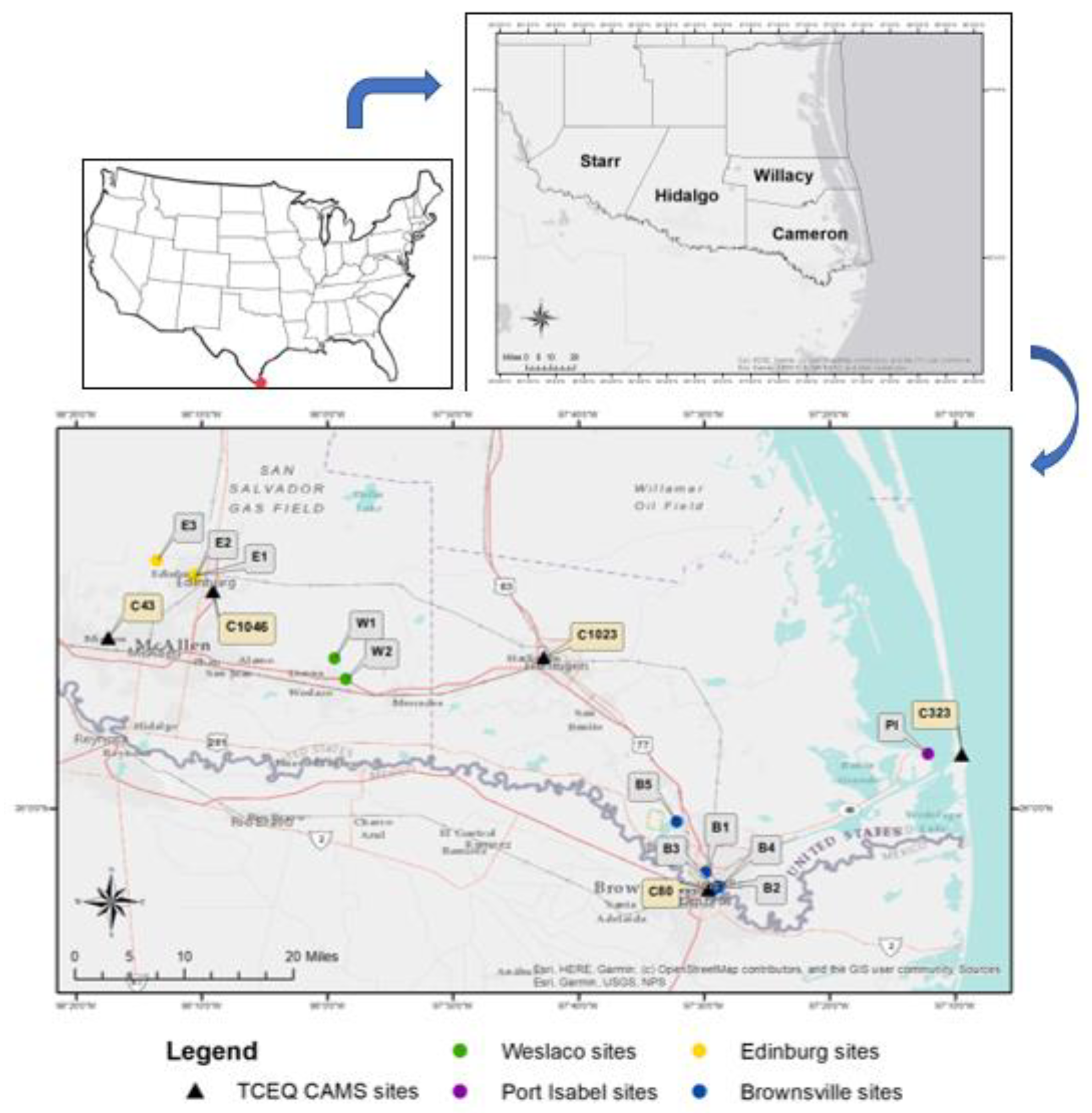
Eleven low-cost sensors (LCSs) were deployed at various sites across the Lower Rio Grande Valley region, i.e., the city of Brownsville, Edinburg, Weslaco, and Port Isabel. Figure 1 shows the Lower RGV region, with color-coordinated locale pinpoints to categorize the LCSs by city. Additionally, the LCSs were labeled based on the city and numbered chronologically. Therefore, the five sensors in the city of Brownsville were labeled B1, B2, B3, B4, and B5 and were shown with deep blue dots. The three LCSs in Edinburg were labeled E1, E2, and E3 with identifying gold-colored dots. In the city of Weslaco, the two LCSs (W1 and W2) were noted as green dots, and lastly, the one LCS in Port Isabel was displayed as a purple dot. The LCSs were placed strategically at various intra-urban locations, i.e., neighborhoods, police departments, and university centers to accurately represent PM exposure burdens. The sensors were installed at the various locations in a manner to not cause any inconvenience to the building or site owners. Additionally, protection from elements, prevention of theft, and availability of electricity outlet were some of the other considerations while choosing the sensors installation locations. The TCEQ CAMS sites were designated with a black triangle marker and labeled according to their identification number, i.e., C43, C80, C323, C1046, and C1023 assigned by the USEPA and TCEQ.
Sensor B1 was deployed in a semi-residential area adjacent to Brownsville’s Gladys Porter Zoo, Dean Porter Park, and the Town Resaca. The household was located on a road roughly 600 m east of the main Texas State Highway (69E). At the University of Texas Rio Grande Valley (UTRGV) Brownsville campus, sensor B2 was positioned outside the campus police department, adjacent to the student dormitories approximately 280 m from the Texas State Highway 69E. The sensor at site B3 was at the UTRGV Music and Science Learning Center Building approximately 22.7 m from a frequently used parking lot, the University Blvd., and the neighboring Lozano Banco Resaca. A resaca, unique geological feature of this area, is typically an ancient distributary channel of the Rio Grande River (the natural international boundary between United States and Mexico in the State of Texas). Lastly, sensor B4 was located at the UTRGV Brownsville campus Vaquero Plaza building about 60 m from the main crossroads where Texas State Highway 69E and University Boulevard intersect. The International Port of Entry (POE) between the United States and Mexico is located further south of Texas State Highway 69E. Site B5 was in a residential household neighborhood bordered by the Resaca del Rancho Viejo.
In the city of Edinburg, sensor E1 was located at the UTRGV-Edinburgh campus’s School of Medicine building approximately 9.8 m from the routinely used W. Schunior St. Similarly, site E2 was deployed at the same University campus at the Student Academic Center 70.3 m off the main intersection of State Highway 107 with Sugar Road. Sensor E3 was located at a gated and secured residential community encircling a resaca.
In the city of Weslaco, sensor W1 was located at a residential home around 164 m near the crossway of Farm to Market Road 88 (FM88). Site W2 was at the Weslaco Police Department building on the frontage of Texas State Expressway 83 adjacent to United States Department of Homeland Security’ s Border Patrol Station in Weslaco and Mid Valley Airport. The sensor PI at Port Isabel City was located at UTRGV’S Coastal Studies Laboratory. Site PI was positioned between two neighborhoods on the coast off the Laguna Madre near the draw bridge connecting Long Island. The study was conducted for a total of 396 days starting from 1 March 2021, and ending on 31 March 2022, to generate a complete year of real-time and continuous PM2.5 data at the eleven sites.
In the Lower RGV region, there were five TCEQ CAMSs active during the study duration. Site C43 is located at John H. Shary Elementary school near an urgent care facility and pediatric clinic in the city of Mission. Site C80 is located at 280 m from the U.S.–Mexican border at the UTRGV Brownsville campus. Site C323 is situated at the UTRGV Coastal labs at the famous resort town of South Padre Islands. This site is in a neighboring trailer park community. The South Padre Island acts as a barrier island against the Gulf of Mexico and connects to the city of Port Isabel via the Queen Isabella Causeway crossing the Laguna Madre. C1046 is stationed on the exterior of the UTRGV Edinburg CESS building off the frontage of Texas State Highway 69C. The C1046 is adjoining a doctor’s office, middle school, and park. Lastly, C1023 is in the city of Harlingen at a High School Freshman Academy. Out of these five CAMS sites, only C43, C80, and C323 monitored PM2.5 during the study period.
2.2. Topography and Meteorological Conditions
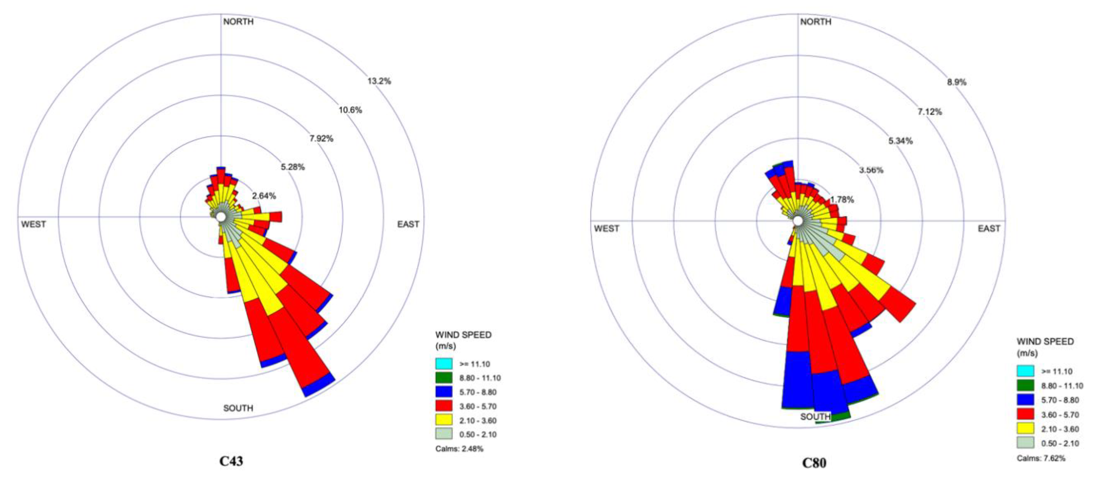
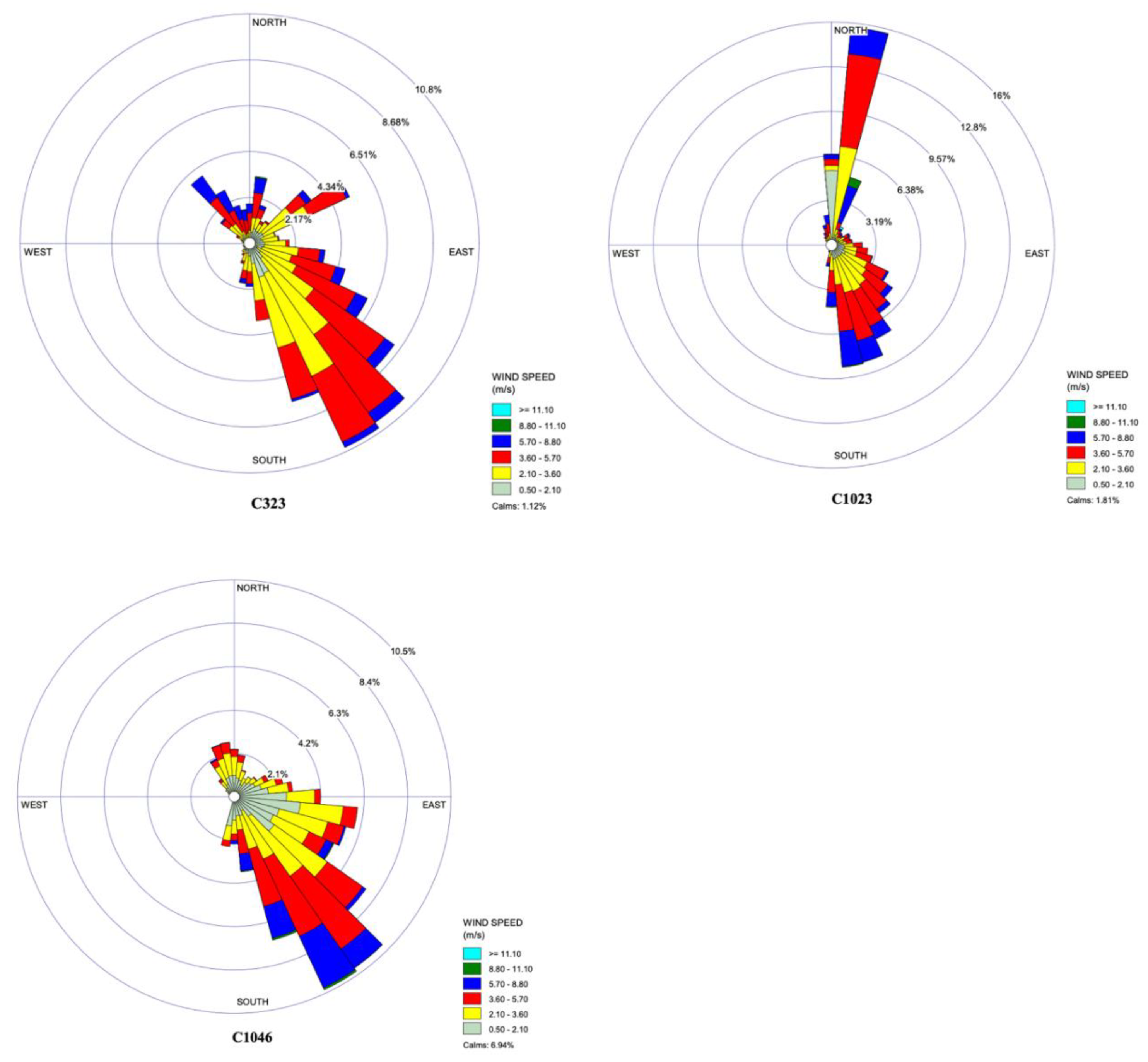
The RGV region’s proximity to the Gulf of Mexico’s warm waters causes a hurricane season ranging from 1 June to 30 November, with increased waters between August and September months [42,43]. Prevailing wind patterns during 1 March 2021, to 31 March 2022, are presented with the help of wind roses for each of the five TCEQ CAMSs, i.e., C43, C80, C323, C1023, and C1046 as shown in Figure 2. Averaged wind speeds were as follows: C43 (2.82 m/s), C80 (3.01 m/s), C323 (3.37 m/s), C1023 (3.55 m/s), and C1046 (2.73 m/s) and were primarily south-easterly for the study period.
Moreover, meteorological parameters from the five TCEQ CAMSs in the Lower RGV region (C43, C80, C323, C1023, and C1046) are summarized in Table 1 for the study period. In order to study the lower RGV weather conditions, meteorological data from all CAMSs were included in the analyses. The average temperature from CAMS was 23 °C for the study duration. The solar radiation expressed the total electromagnetic radiation at stations C43 (0.3) and C80 (0.3) in Langley’s per minute.
2.3. Instrumentation
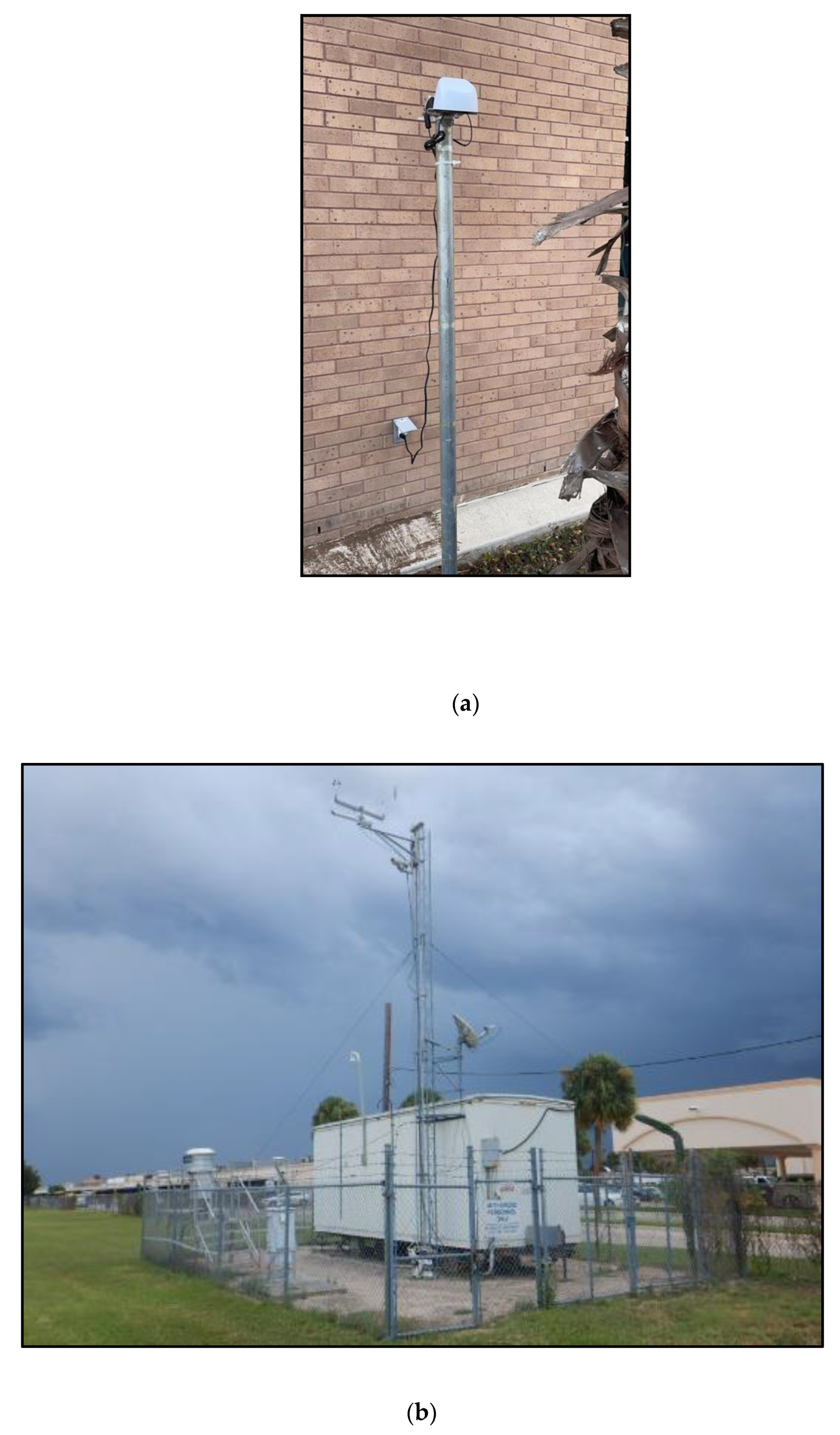
The LCSs used in this research study were BlueSky™ Air Quality Monitors, TSI Inc., Shoreview, MN, USA (Model: 8143). Figure 3a shows a picture of the BlueSky™ sensor at one of the study locations. For comparative assessment, Figure 3b shows the location of the TCEQ CAMS C43 site. These sensors include a six-channel particulate counter to measure particulate matter mass concentrations and additional parameters, i.e., temperature and relative humidity. The aerosol mass concentrations are depicted from 0 to 1000 μg/m3, with a measurement resolution of 1 μg/m3 [52]. Furthermore, the PM sensor is pre-calibrated with a self-diagnostic ability to attain performance with more than 95% up-time and acquire high-quality real-time data [53]. For the purposes of this paper, we have presented only PM2.5 data. PM2.5 (µg/m3) concentrations were collected at five-minute intervals and converted into hourly concentrations for the analyses.
2.4. Quality Assurance and Quality Control (QA/QC) of PM2.5 Data
Standard data quality assurance procedures from the USEPA [15,16,55] were implemented in this study. Completeness was calculated by dividing the observed samples by the targeted samples [29,30]. In this study, the targeted sample amount is 396 days or the complete study duration. PM2.5 24 h completeness values for all the LCSs were >89.4%, while the TCEQ CAMSs were C43 (99.2%), C80 (99.0%), and C323 (88.9%) as shown in Table 2. Few instances of data loss were attributed to a variety of reasons such as power outages and/or PM sensor errors or malfunctions.
QA/QC studies were conducted between a few samplers, both before and after the study period. Coefficient of determination (R2) values from a linear regression model between two sensors were computed along with their respective slope and intercepts [56]. R2 is the correlation between two sensor outputs and the slope provides information on their magnitudes.
Precision was also determined for the samplers. Typically, it represents the reproducibility of measurements as determined by collocated sampling using the same methods or by propagation of individual measurement errors determined by replicate analysis, blank analysis, and performance tests [56]. Precision for a set of repeated data, si, is defined as deviation from the average response to the same measurable quantity as follows:
where Ci,j is the jth measured concentration for the ith set of data; Ci,average is the average concentration for the ith set of data; and m is the number of repeated measurements for the selected sample set i.
For a particular set of paired duplicate samples, j = 2 and Ci,average = (Ci,1 + Ci,2)/2
where Δi is the difference between the two collocated samples for set i.
The absolute precision for a group of data that is composed of multiple sets of duplicate samples collected from different locations at different time, s, is defined as follows [57,58,59]:
The overall relative precision, p, can be expressed in percentage of the mean observations and the goal is set at ±10%:
Table 3 provides the details about the pre- and the post-study QA/AC analyses. The near unity R2 values indicate high reproducibility between the sensors, and they compare well amongst each other. Calculations were based on hourly averaged data. The Root Mean Squared Difference (RMSD) and relative precision values were as expected and in line with reported in literature for low-cost sensors [60]. RMSD values varied from 0.58 to 3.05 µg/m3 for this pre- and post-study QA/AC campaign. Laboratory and field studies conducted by the South Coast Air Quality Management District on BlueSky sensors have also shown a moderate to strong correlations (0.66 < R2 < 0.78) with other FEM instruments such as GRIMM and Teledyne API T640 [61]. Relative precision ranged from 4 to 30.5%. Typically, in air quality academic literature, a ±10% relative precision is aimed for. The higher relative precision percentage values are from the post-study session (sensors B3-W1 and E1-E3) whereas most of the pre-study session precision rates are within the recommended range. If all the four pre-study precision test sessions are combined (due to it being the same sensor pairs, W1-B5, and same test location), the relative precision is 8%. This instills a level of confidence in the overall quality of our study data.
We also computed the Spearman’s Rho (r) and Coefficient of Divergence (COD) values for the sensor pairs as shown in Figure 3. CODs are typically computed to characterize the spatial heterogeneity in pollutant concentrations between two simultaneously sampled sites or locations. The COD provides a degree of uniformity between two simultaneously sampled sites, j and k:
where Xij represents the ith concentration measured at site j over the study duration, and the number of observations is p [29,30,62,63,64]. A low COD value (r < 0.2) indicates similar pollutant concentrations between two sites, whereas a value approaching unity indicates substantial difference in the absolute concentrations and confirms spatial heterogeneity between the two sites or two collocated samplers at one specific location. As anticipated, the Spearman’s Rho values between the paired sensors, both pre-and post-study, were all above 0.986 suggesting consistency in the measurements. Similarly, the COD values between the paired sensors were well all below 0.2 (ranging from 0.032 to 0.177) demonstrating that sensor precision.
We did not incorporate any calibration factor to the PM2.5 database. The BlueSky™ sensors comes factory pre-calibrated and compares well the other high-quality Federal Equivalent Method TSI equipment such as the DustTrak™ series (TSI Incorporated, Shoreview, MN, USA). Self-diagnostic tests were configured to daily cleaning intervals to attain high-quality data during the study period. We would be remiss, however, if some of the limitations and challenges associated with the usage of low-cost sensors in the air quality field are not mentioned here. Currently, there is a smorgasbord of such low-cost sensors in the market. Issues associated with accuracy, missing data, baseline drift, effects of temperature and relative humidity are some, if not all, the parameters plaguing the efficacy of these sensors [65,66,67] Technological advancement in the field of low-cost sensors in the coming years will hopefully ameliorate some of these limitations.
“Furthermore, in an ideal scenario, comparison of the sensors used in this study should have been collocated with the three TCEQ CAMS sites at the beginning of the study. However, the study was conceived during the peak COVID-19 pandemic period and that presented many logistical challenges due to lockdowns etc. We recommend that future studies by ours as well as other research groups in this region should undertake the sensor comparisons with the TCEQ CAMS sites itself (i.e., installing the sensors in the vicinity or the premises of the TCEQ CAMS sites) pursuant to getting the requisite permission from the government authorities in the city and county and, perhaps, limiting the scope of the study in terms of area and duration. i.e., conducting a study with multiple low-cost sensors within a single city.”
2.5. Statistical Data Analysis
Fine particulate matter concentrations from the eleven LCSs were processed for spatial and temporal analyses along with the data obtained from the three TCEQ CAMS sites. Descriptive statistics were carried out in Microsoft Excel (v.16.06, Microsoft Inc., Redmond, WA, USA), R programming software (RStudio, Inc., Boston, MA, USA), and SPSS for MacOS (SPSS, Inc., Chicago, IL, USA). A conditional (TRUE and FALSE) IF statement was used in Excel to clean the raw data by flagging any inconsistencies with the automated 5 min interval settings. Hence, any missing data points were accounted for in the data set by the addition of blank rows. Subsequently, the cleaned 5 min data were converted to hourly and 24 h data. Box and whisker plots and time series were procured to demonstrate PM2.5 variability from both LCSs and TCEQ CAMS sites.
Site-specific temporal relationships were assessed with Spearman’s Rho correlations with a significance level set at 0.01. Spatial variation between the eleven sampled sites and the three TCEQ CAMS sites was analyzed by using the Coefficient of Divergence (COD) analyses.
3. Results and Discussion
3.1. PM2.5 Concentration Analyses
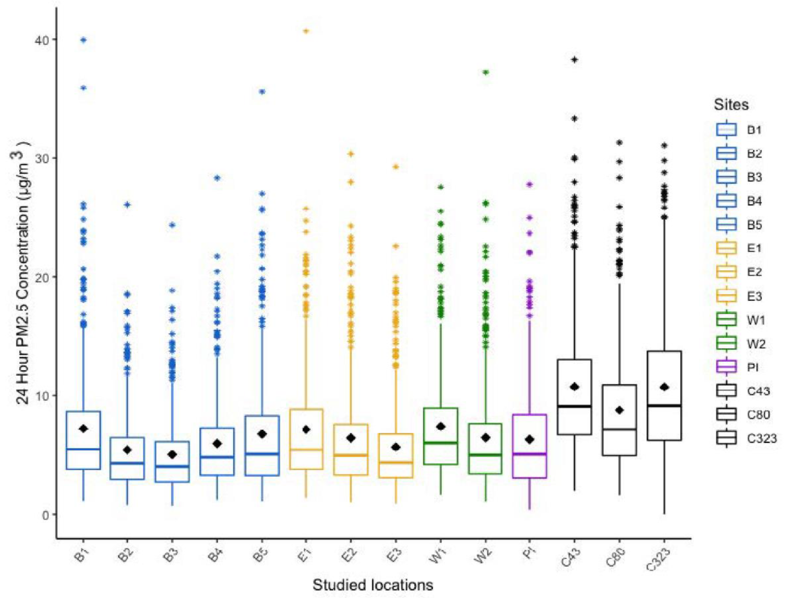
The box and Whisker plot for PM2.5 24 h concentrations (μg/m3) for the eleven LCSs and three CAMS sites for the entire study duration is shown in Figure 4. The Brownsville sites B1, B2, B3, B4, and B5 are shown in deep blue, E1, E2, and E3 are shown in gold for the city of Edinburg; sites W1 and W2 located in the city of Weslaco are shown in green; and lastly, site PI at Port Isabel is shown in purple. The three CAMS sites, C43, C80, and C323, are shown in black. Descriptive statistics of 24 h ambient PM2.5 concentrations (μg/m3) from the LCS sites and the three CAMSs (C43, C80, and C323) are presented in Table 4. Each LCS site was chosen to accurately represent daily intra- and inter-urban PM2.5 exposures at the neighborhood level.
Mean (SD) PM2.5 concentrations in the city of Brownsville varied with the highest mean value of 8.79 (5.39) µg/m3 at C80. Site B1 recorded an average of 7.24 (5.39) µg/m3 for the study period. The UTRGV Brownsville campus sites showed slightly lower concentrations: site B3, 5.05 (3.35) µg/m3 and site B4, 5.99 (4.01) µg/m3, when compared to the residential areas at site B5, 6.77 (5.17) µg/m3. The sensors at the city of Edinburg had concentrations ranging from 5.69 (4.08) µg/m3 in the gated residential community site, E3, to 7.16 (4.97) µg/m3 at the UTRGV medical building facing W Schunior St, E1, and 6.45 (4.78) µg/m3 at site E2. The two sites in Weslaco city recorded almost similar mean values for the study period: site W1, located right off FM Road 88, 7.43 (4.68) µg/m3 and site W2 off Texas State Highway 69, 6.47 (4.79) µg/m3.
The PM2.5 concentrations at CAMS site C43 located outside an elementary school was the highest for the study period: 10.76 (5.81) µg/m3. Similarly, CAMS site C323 at the UTRGV coastal labs in South Padre Island recorded an average of 10.74 (6.00) µg/m3, which was more than what was recorded at Site PI, 6.33 (4.54) µg/m3. The residential household near the crossroads of FM88, site W2, recorded average PM2.5 concentration of 7.43 (4.68) µg/m3.
The PM2.5 averages for all sites were less than 15 μg/m3, and the outliers were less than 45 μg/m3. According to the latest National Ambient Air Quality Standards (NAAQS), mandated under Sections 108 and 109 of the U.S. Clean Air Act of 1970, and amendments thereof in 1990, the average PM2.5 concentrations from this study did not exceed the 24 h mean threshold of 35 µg/m3 [15]. Similarly, the findings from this study did not surpass the PM2.5 daily concentration average threshold of 15 µg/m3 from the Worlds Health Organization’s (WHOs) global air quality guidelines of 2021 [20]. The eleven LCSs and the three CAMSs were just within these designated standards throughout the study duration. Thresholds for criteria pollutants such as fine particulate matter are designated for the protection of the community’s health and welfare.
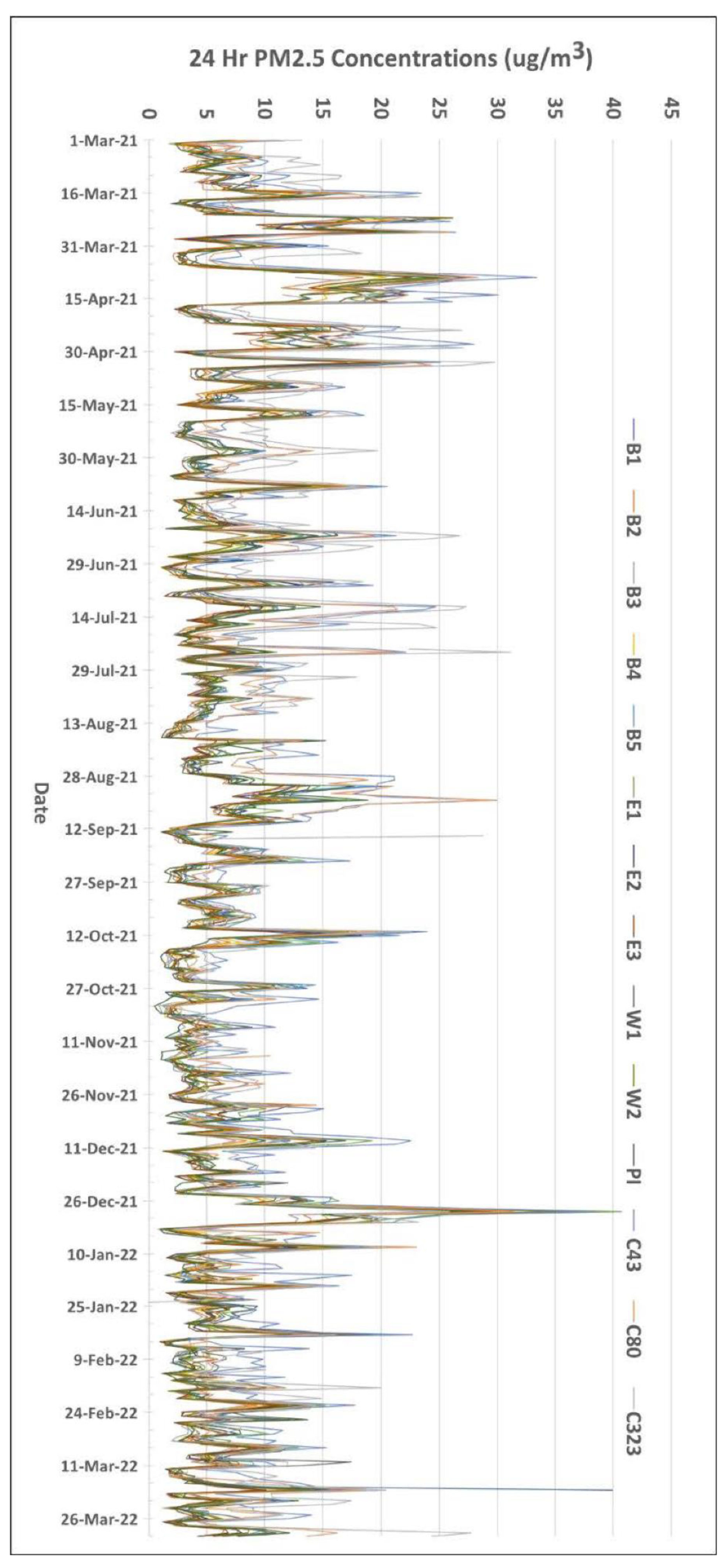
Figure 5 shows the time series for the 24 h PM2.5 concentrations for the study period from 1 March 2021, to 31 March 2022, at the eleven study sites and the three CAMS locations. These temporal patterns observed across the four cities reveal a similar pattern albeit with varying absolute concentrations. High peak levels were ubiquitous throughout the study landscape from 23 December 2021 to 3 January 2022. This could, perhaps, be attributed to Christmas and New Year festivities, which are typically celebrated with firework displays and outdoor cookouts—a trend also seen during the 4 July US Independence Day weekend.
3.2. Spatial Heterogeneity across the Four Cities
Spatial heterogeneity in PM2.5 concentrations across the eleven sampled sites and three CAMS sites in the four cities are shown as a COD matrix in Table 5. COD values illustrated in bold italics are greater than 0.20 suggesting spatial heterogeneity between the sites. CAMS sites C43, C80, and C323 confirm spatial non-uniformity, with the eleven LCSs with COD values ranging from 0.25 (C80-W2) to 0.58 (C323-B2). For CAMS site C323, spatial non-uniformity was also pronounced when paired with sites B3 (0.54), B4 (0.5), and E3 (0.5). Spatial variability was also observed between site B2 and CAMS sites with high COD values: C43-B2(0.49), and C80-B2(0.43). In the city of Edinburg, site E3 also exhibited variation in pollutant concentrations when paired with various CAMS sites: C43(0.38), C80(0.31), and C323(0.5). In the city of Weslaco (W1 and W2), the CAMSs indicated spatial non-homogeneity with COD values greater than 0.25. Additionally, at Port Isabel, absolute pollutant concentrations at site (PI) reflected spatial non-homogeneity when paired with the three CAMS sites with COD values ranging between 0.37 (C43), 0.28 (C80), and 0.47 (C323).
Intra-city spatial homogeneity, as indicated by COD values < 0.2, was also observed for site-pairings within Edinburg such as E2-E1 (0.16), E3-E2 (0.11), and (0.20) E3-E1. Similarly, spatial uniformity in PM2.5 absolute concentrations was observed for the following inter-city sites pairings: W2-E1 (0.17), W2-E2 (0.10), W2-E3 (0.14), and PI-W2 (0.19). All of the sites’ pairings between the cities of Brownsville and Edinburg also demonstrated a moderate degree of variation in pollutant concentrations with COD values ranging from 0.20 to 0.40. Overall, COD values from this study demonstrate that federal and state ambient monitoring sites may not accurately reflect the PM2.5 burden patterns of the population resulting in potential exposure misclassifications, thereby confirming the importance of neighborhood level monitoring as accomplished in this study using LCSs.
3.3. Inter-Site Correlation Analyses
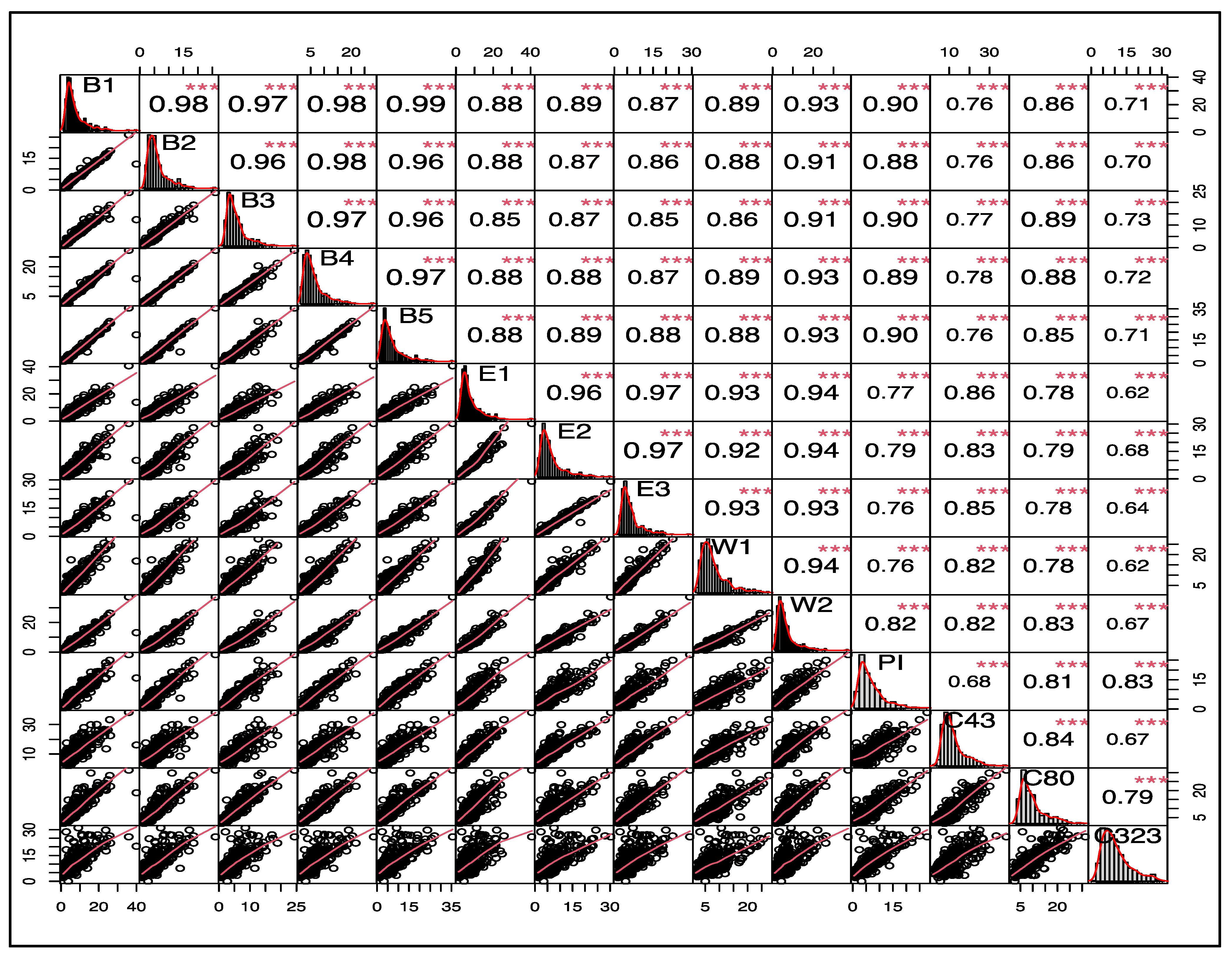
Inter-site correlation analyses were undertaken between the sampled and TCEQ CAMS sites to characterize the PM2.5 temporal patterns for the study duration. The correlation coefficient values computed as Spearman’s Rho are shown in a matrix in Figure 6. The Spearman’s Rho correlations plot also show the density functions, histograms, and smoothed regression analysis. Histogram curves and regression analyses corroborate the similarity in temporal relationships between all the sampled and TCEQ CAMS sites.
Statistical significance was set at 0.01 level (represented by **). Stronger relationships between the sites are indicated as coefficients approaching unity, whereas values near zero suggest weak to no correlations. Correlations were strong and statistically significant when the eleven sites were paired amongst each other (0.76 < r < 0.99). Correlations coefficients for the CAMS and eleven study sites pairing also yielded strong and significant correlations (0.62 < r < 0.89). Specifically, the five sites in Brownsville were very strongly correlated with each other (r > 0.96). C80 was also strongly correlated with these five Brownsville study locations (0.85 < r < 0.89). In the city of Edinburg, the three study sites (E1, E2, and E3) showed a robustly strong temporal relationship with r > 0.96. Similarly, a Spearman’s Rho value of 0.95 was obtained for the two Weslaco W1 and W2. The Port Isabel site, PI, yielded a moderately high temporality with C43 (r = 0.68). These correlation coefficients indicate that the pollutant concentrations across all the sites and the CAMS sites exhibited a strong temporal relationship.
Taken together, these temporal and spatial patterns observed between the various sites during the study duration between the various study locations and TCEQ Sites, as well as between the paired sensors during the pre-and post-study period confirm the differences in sites in terms of pollutant concentrations rather than the differences being attributable to the functioning of the sensors used in this study.
4. Conclusions
The findings from this study are the first of its type in the Lower Rio Grande Valley region in South Texas, characterizing PM2.5 exposures at the intra- and- inter- urban level for a year with low-cost sensors deployed in multiple towns and cities, i.e., Brownsville, Edinburg, Weslaco, and Port Isabel. This research work will contribute toward future air quality evaluations in this part of the U.S.–Mexico border region. The study assessed PM2.5; however, future air quality campaigns in this region could also involve other criteria air pollutants such as NO2, CO, and O3. This will help determine the different exposure burden patterns for these gaseous pollutants. The latest technological advances in the field of low-cost sampling of various pollutants would help achieve this goal. The rapid developments with the low-cost sensors combined with the central ambient monitoring sites will enhance community monitoring for real-time spatial and temporal pollutant patterns. The study findings from this air quality campaign and future such studies have the potential to provide vital air quality knowledge to the local citizenry. In this study, the daily averaged PM2.5 concentrations throughout this study were within the designated guidelines by the NAAQS and WHO. Short-term daily PM2.5 levels were, however, high at times potentially causing respiratory health issues attributed to this pollutant.
The findings from this study are important also due to the COVID-19 pandemic that primarily affected the human respiratory system. PM2.5 exposures result in acute and chronic health effects that would only intensify when paired with the pandemic health effects. Finally, future studies in this region should also explore the possibility of conducting similar air monitoring campaigns with low-cost sensors on the other side of the international border. This seems to be unfortunately unlikely for now due to high cartel violence plaguing cities and towns on the other side of the border in Mexican states such as Tamaulipas, Nueva Leon. However, once the security situation improves, a possibility should be forged by future research groups to conduct a binational air monitoring campaign to study criteria air pollutants using low-cost sensors. This will increase the air quality knowledge of the local population, contribute toward the various emissions inventories for this region, as well as demonstrate that issues such as air pollution recognize no human-made jurisdictions and issues pertaining to human exposures need to be addressed in a holistic manner by involving local and state stakeholders on both sides of the international border.
Author Contributions
A.U.R., D.W., K.S. and O.T. conceived and designed the study; E.M. implemented the study; A.U.R., O.T. and E.M. supervised the data collection; E.M. analyzed the data and wrote the initial draft of the manuscript; A.U.R. edited and prepared the final draft. D.W., K.S. and O.T. gave valuable comments on the initial draft. All authors provided valuable comments and ideas while drafting the manuscript. All authors have read and agreed to the published version of the manuscript.
Funding
Funding for this research work was kindly provided by the UTRGV under the new faculty startup funds given to A.U.R. Graduate assistantship for E.M. was generously provided by the School of Earth, Environment, and Marine Sciences, UTRGV.
Institutional Review Board Statement
Not applicable.
Informed Consent Statement
Not applicable.
Data Availability Statement
Data available upon request.
Acknowledgments
The authors express their appreciation to David Mendez for his help with this study’s fieldwork. The authors also thank the two anonymous reviewers for their insightful comments and constructive suggestions that helped improve our research manuscript. Additionally, this study neither promotes nor endorses the usage of TSI BlueSky™ sensors.
Conflicts of Interest
The authors declare no conflict of interest.
References
- Feenstra, B.J. Development of Methodologies for the Use and Application of Air Quality Sensors to Enable Community Air Monitoring. Ph.D. Thesis, University of California, Riverside, CA, USA, 2020. [Google Scholar]
- Gao, M.; Cao, J.; Seto, E. A distributed network of low-cost continuous reading sensors to measure spatiotemporal variations of PM2.5 in Xi’an, China. Environ. Pollut. 2015, 199, 56–65. [Google Scholar] [CrossRef] [PubMed]
- Lee, C.-H.; Wang, Y.-B.; Yu, H.-L. An efficient spatiotemporal data calibration approach for the low-cost PM2.5 sensing network: A case study in Taiwan. Environ. Int. 2019, 130, 104838. [Google Scholar] [CrossRef] [PubMed]
- Liu, X.; Jayaratne, R.; Thai, P.; Kuhn, T.; Zing, I.; Christensen, B.; Lamont, R.; Dunbabin, M.; Zhu, S.; Gao, J.; et al. Low-cost sensors as an alternative for long-term air quality monitoring. Environ. Res. 2020, 185, 109438. [Google Scholar] [CrossRef] [PubMed]
- Mukherjee, A.; Stanton, L.G.; Graham, A.R.; Roberts, P.T. Assessing the Utility of Low-Cost Particulate Matter Sensors over a 12-Week Period in the Cuyama Valley of California. Sensors 2017, 17, 1805. [Google Scholar] [CrossRef]
- Wang, Z. Long-Term Evaluation of Low-Cost Air Sensors in Monitoring Indoor Air Quality at a California Community. Master’s Thesis, University of California, Los Angeles, CA, USA, 2020. [Google Scholar]
- deSouza, P.N.; Nthusi, V.K.; Klopp, J.; Shaw, B.E.; Ho, W.O.; Saffell, J.; Jones, R.L.; Ratti, C. A Nairobi experiment in using low cost air quality monitors. Clean Air J. 2017, 27, 12. [Google Scholar] [CrossRef]
- Pang, X.; Chen, L.; Shi, K.; Wu, F.; Chen, J.; Fang, S.; Wang, J.; Xu, M. A lightweight low-cost and multipollutant sensor package for aerial observations of air pollutants in atmospheric boundary layer. Sci. Total Environ. 2021, 764, 142828. [Google Scholar] [CrossRef]
- Khreis, H.; Johnson, J.; Jack, K.; Dadashova, B.; Park, E.S. Evaluating the Performance of Low-Cost Air Quality Monitors in Dallas, Texas. Int. J. Environ. Res. Public Health 2022, 19, 1647. [Google Scholar] [CrossRef]
- Sun, L.; Wong, K.C.; Wei, P.; Ye, S.; Huang, H.; Yang, F.; Westerdahl, D.; Louie, P.K.K.; Luk, C.W.Y.; Ning, Z. Development and Application of a Next Generation Air Sensor Network for the Hong Kong Marathon 2015 Air Quality Monitoring. Sensors 2016, 16, 211. [Google Scholar] [CrossRef]
- Weissert, L.F.; Salmond, J.A.; Miskell, G.; Alavi-Shoshtari, M.; Grange, S.K.; Henshaw, G.S.; Williams, D.E. Use of a dense monitoring network of low-cost instruments to observe local changes in the diurnal ozone cycles as marine air passes over a geographically isolated urban centre. Sci. Total Environ. 2017, 575, 67–78. [Google Scholar] [CrossRef]
- Zamora, M.L.; Rice, J.; Koehler, K. One Year Evaluation of Three Low-Cost PM(2.5) Monitors. Atmos. Environ. 2020, 235, 117615. [Google Scholar] [CrossRef]
- Esworthy, R. Air Quality: EPA’S 2013 Changes to the Particulate Matter (PM) Standard; CreateSpace: Scotts Valley, CA, USA, 2014; pp. 157–208. [Google Scholar]
- Kim, K.-H.; Kabir, E.; Kabir, S. A review on the human health impact of airborne particulate matter. Environ. Int. 2015, 74, 136–143. [Google Scholar] [CrossRef] [PubMed]
- United States Environmental Protection. NAAQS Table. Available online: https://www.epa.gov/criteria-air-pollutants/naaqs-table (accessed on 14 May 2022).
- Particulate Matter (PM) Pollution. Available online: https://www.epa.gov/pm-pollution/particulate-matter-pm-basics (accessed on 14 May 2022).
- Burton, R.K. Analysis of Low-Cost Particulate Matter Shinyei Sensor for Asthma Research. Master’s Thesis, University of Maryland, Baltimore, MD, USA, 2017. [Google Scholar]
- Dausman, T.B.C. Low Cost Air Quality Monitors in Agriculture. Master’s Thesis, The University of Iowa, Iowa City, IA, USA, 2017. [Google Scholar]
- Srimuruganandam, B.; Shiva Nagendra, S.M. Source characterization of PM10 and PM2.5 mass using a chemical mass balance model at urban roadside. Sci. Total Environ. 2012, 433, 8–19. [Google Scholar] [CrossRef] [PubMed]
- Ambient (Outdoor) Air Pollution. Available online: https://www.who.int/news-room/fact-sheets/detail/ambient-(outdoor)-air-quality-and-health (accessed on 13 May 2022).
- Atkinson, R.W.; Fuller, G.W.; Anderson, H.R.; Harrison, R.M.; Armstrong, B. Urban Ambient Particle Metrics and Health: A Time-series Analysis. Epidemiology 2010, 21, 501–511. [Google Scholar] [CrossRef] [PubMed]
- Brunekreef, B.; Forsberg, B. Epidemiological evidence of effects of coarse airborne particles on health. Eur. Respir. J. 2005, 26, 309–318. [Google Scholar] [CrossRef] [PubMed]
- Cadelis, G.; Tourres, R.; Molinie, J. Short-Term Effects of the Particulate Pollutants Contained in Saharan Dust on the Visits of Children to the Emergency Department due to Asthmatic Conditions in Guadeloupe (French Archipelago of the Caribbean). PLoS ONE 2014, 9, e91136. [Google Scholar] [CrossRef]
- Correia, A.W.; Pope, C.A., 3rd; Dockery, D.W.; Wang, Y.; Ezzati, M.; Dominici, F. Effect of air pollution control on life expectancy in the United States: An analysis of 545 U.S. counties for the period from 2000 to 2007. Epidemiology 2013, 24, 23–31. [Google Scholar] [CrossRef]
- Fang, Y.; Naik, V.; Horowitz, L.W.; Mauzerall, D.L. Air pollution and associated human mortality: The role of air pollutant emissions, climate change and methane concentration increases from the preindustrial period to present. Atmos. Chem. Phys. 2013, 13, 1377–1394. [Google Scholar] [CrossRef]
- Meister, K.; Johansson, C.; Forsberg, B. Estimated short-term effects of coarse particles on daily mortality in Stockholm, Sweden. Environ. Health Perspect. 2012, 120, 431–436. [Google Scholar] [CrossRef]
- Misra, C.; Geller, M.; Shah, P.; Solomon, P. Development and evaluation of a continuous coarse (PM10-PM2.5) particle monitor. J. Air Waste Manag. Assoc. 2001, 51, 1309–1317. [Google Scholar] [CrossRef]
- de Kok, T.M.; Driece, H.A.; Hogervorst, J.G.; Briedé, J.J. Toxicological assessment of ambient and traffic-related particulate matter: A review of recent studies. Mutat. Res. 2006, 613, 103–122. [Google Scholar] [CrossRef]
- Raysoni, A.U.; Sarnat, J.A.; Sarnat, S.E.; Garcia, J.H.; Holguin, F.; Luèvano, S.F.; Li, W.-W. Binational school-based monitoring of traffic-related air pollutants in El Paso, Texas (USA) and Ciudad Juárez, Chihuahua (México). Environ. Pollut. 2011, 159, 2476–2486. [Google Scholar] [CrossRef] [PubMed]
- Raysoni, A.U.; Stock, T.H.; Sarnat, J.A.; Montoya Sosa, T.; Ebelt Sarnat, S.; Holguin, F.; Greenwald, R.; Johnson, B.; Li, W.-W. Characterization of traffic-related air pollutant metrics at four schools in El Paso, Texas, USA: Implications for exposure assessment and siting schools in urban areas. Atmos. Environ. 2013, 80, 140–151. [Google Scholar] [CrossRef]
- Askariyeh, M.H.; Venugopal, M.; Khreis, H.; Birt, A.; Zietsman, J. Near-Road Traffic-Related Air Pollution: Resuspended PM2.5 from Highways and Arterials. Int. J. Environ. Res. Public Health 2020, 17, 2851. [Google Scholar] [CrossRef] [PubMed]
- Girguis, M.S.; Strickland, M.J.; Hu, X.; Liu, Y.; Bartell, S.M.; Vieira, V.M. Maternal exposure to traffic-related air pollution and birth defects in Massachusetts. Environ. Res. 2016, 146, 1–9. [Google Scholar] [CrossRef] [PubMed]
- Kioumourtzoglou, M.A.; Schwartz, J.D.; Weisskopf, M.G.; Melly, S.J.; Wang, Y.; Dominici, F.; Zanobetti, A. Long-term PM2.5 Exposure and Neurological Hospital Admissions in the Northeastern United States. Environ. Health Perspect. 2016, 124, 23–29. [Google Scholar] [CrossRef] [PubMed]
- Vallamsundar, S.; Askariyeh, M.H.; Zietsman, J.; Ramani, T.L.; Johnson, N.M.; Pulczinski, J.; Koehler, K.A. Maternal Exposure to Traffic-Related Air Pollution Across Different Microenvironments. J. Transp. Health 2016, 3, S72. [Google Scholar] [CrossRef]
- Weinstock, L.; Watkins, N.; Wayland, R.; Baldauf, R. EPA’s Emerging Near-Road Ambient Monitoring Network: A Progress Report. EM Magazine. 2013. Available online: pubs.awma.org/gsearch/em/2013/7/weinstock.pdf (accessed on 20 May 2022).
- Bozlaker, A.; Buzcu-Güven, B.; Fraser, M.P.; Chellam, S. Insights into PM10 sources in Houston, Texas: Role of petroleum refineries in enriching lanthanoid metals during episodic emission events. Atmos. Environ. 2013, 69, 109–117. [Google Scholar] [CrossRef]
- Bozlaker, A.; Spada, N.J.; Fraser, M.P.; Chellam, S. Elemental characterization of PM2.5 and PM10 emitted from light duty vehicles in the Washburn Tunnel of Houston, Texas: Release of rhodium, palladium, and platinum. Environ. Sci. Technol. 2014, 48, 54–62. [Google Scholar] [CrossRef]
- Juda-Rezler, K.; Reizer, M.; Oudinet, J.-P. Determination and analysis of PM10 source apportionment during episodes of air pollution in Central Eastern European urban areas: The case of wintertime 2006. Atmos. Environ. 2011, 45, 6557–6566. [Google Scholar] [CrossRef]
- Kulkarni, P.; Chellam, S.; Fraser, M.P. Lanthanum and lanthanides in atmospheric fine particles and their apportionment to refinery and petrochemical operations in Houston, TX. Atmos. Environ. 2006, 40, 508–520. [Google Scholar] [CrossRef]
- Kulkarni, P.; Chellam, S.; Fraser, M.P. Tracking petroleum refinery emission events using lanthanum and lanthanides as elemental markers for PM2.5. Environ. Sci. Technol. 2007, 41, 6748–6754. [Google Scholar] [CrossRef]
- Williamson, K.; Das, S.; Ferro, A.R.; Chellam, S. Elemental composition of indoor and outdoor coarse particulate matter at an inner-city high school. Atmos. Environ. 2021, 261, 118559. [Google Scholar] [CrossRef]
- Mendez, E.; Rodriguez, J.; Luna, A.; Raysoni, A.U. Comparative Assessment of Pollutant Concentrations and Meteorological Parameters from TCEQ CAMS Sites at Houston and Rio Grande Valley Regions of Texas, USA in 2016. Open J. Air Pollut. 2022, 11, 13–27. [Google Scholar] [CrossRef]
- The Official South Texas Hurricane Guide. 2021. Available online: https://www.weather.gov/media/crp/2021_HG_English_Final.pdf (accessed on 14 May 2022).
- Rio Grande Valley, Texas Travel Guide. Available online: https://www.go-texas.com/Rio-Grande-Valley/ (accessed on 14 May 2022).
- Karnae, S.; John, K. Source apportionment of PM2.5 measured in South Texas near U.S.A—Mexico Border. Atmos. Pollut. Res. 2019, 10, 1663–1676. [Google Scholar] [CrossRef]
- Akland, G.G.; Schwab, M.; Zenick, H.; Pahl, D. An interagency partnership applied to the study of environmental health in the Lower Rio Grande Valley of Texas. Environ. Int. 1997, 23, 595–609. [Google Scholar] [CrossRef]
- North American Free Trade Agreement (NAFTA). Available online: https://www.trade.gov/north-american-free-trade-agreement-nafta (accessed on 14 May 2022).
- U.S.-Mexico Border Program. Available online: https://www.epa.gov/usmexicoborder/what-border-2025 (accessed on 14 May 2022).
- Population Data for Region: Rio Grande Valley. Available online: https://www.rgvhealthconnect.org/demographicdata?id=281259§ionId=935 (accessed on 14 May 2022).
- Lusk, M.; Staudt, K.; Moya, E.M. Chapter 1: Social Justice in the U.S.-Mexico Border Region 2012; Springer: Dordrecht, The Netherlands; Heidelberg, Germany; New York, NY, USA; London, UK, 2012; ISBN 978-94-007-4150-8. [Google Scholar] [CrossRef]
- QuickFacts Hidalgo County, Texas; Cameron County, Texas. Available online: https://www.census.gov/quickfacts/fact/table/hidalgocountytexas,cameroncountytexas/IPE120220#IPE120220 (accessed on 15 May 2022).
- BlueSky Air Quality Monitor. Available online: https://tsi.com/getmedia/4c72a030-4585-4df4-a7c8-596aa1994734/BlueSky-Air-Quality-Monitor_A4_5002492_RevB_Web?ext=.pdf (accessed on 15 May 2022).
- TSI-BlueSky. Available online: http://www.aqmd.gov/aq-spec/sensordetail/tsi---bluesky (accessed on 15 May 2022).
- TCEQ CAMS 43 Location. Available online: https://www17.tceq.texas.gov/tamis/index.cfm?fuseaction=report.view_site&siteID=97&siteOrderBy=name&showActiveOnly=0&showActMonOnly=1&formSub=1&tab=pics (accessed on 10 September 2022).
- United States Environmental Protection Agency. EPA Requirements for Quality Assurance Project Plans: EPA/240/B-01/003. Available online: https://www.epa.gov/sites/default/files/2016-06/documents/r5-final_0.pdf (accessed on 14 May 2022).
- Zou, Y.; Clark, J.D.; May, A.A. Laboratory evaluation of the effects of particle size and composition on the performance of integrated devices containing Plantower particle sensors. Aerosol Sci. Technol. 2021, 55, 848–858. [Google Scholar] [CrossRef]
- Hoek, G.; Brunekreef, B.; Goldbohm, S.; Fischer, P.; van den Brandt, P.A. Association between mortality and indicators of traffic-related air pollution in the Netherlands: A cohort study. Lancet 2002, 360, 1203–1209. [Google Scholar] [CrossRef]
- Lewne, M.; Cyrys, J.; Meliefste, K.; Hoek, G.; Brauer, M.; Fischer, P. Spatial variation in nitrogen dioxide in three European areas. Sci. Total Environ. 2004, 332, 217–230. [Google Scholar] [CrossRef]
- Sarnat, J.A.; Koutrakis, P.; Suh, H.H. Assessing the relationship between personal particulate and gaseous exposures of senior citizens living in Baltimore, MD. J. Air Waste Manag. Assoc. 2000, 50, 1184–1198. [Google Scholar] [CrossRef]
- Morawska, L.; Thai, P.K.; Liu, X.; Asumadu-Sakyi, A.; Ayoko, G.; Bartonova, A. Applications of low-cost sensing technologies for air quality monitoring and exposure assessment: How far have they gone? Environ. Int. 2018, 116, 286–299. [Google Scholar] [CrossRef]
- AQMD Air Quality Sensor Performance Evaluation Center. 2021. Available online: http://www.aqmd.gov/aq-spec/evaluations/summary-pm (accessed on 19 May 2022).
- Pinto, J.P.; Lefohn, A.S.; Shadwick, D.S. Spatial variability of PM2.5 in urban areas in the United States. J. Air Waste Manag. Assoc. 2004, 54, 440–449. [Google Scholar] [CrossRef]
- Krudysz, M.A.; Froines, J.R.; Fine, P.M.; Sioutas, C. Intra-community spatial variation of size-fractionated PM mass, OC, EC, and trace elements in the Long Beach, CA area. Atmos. Environ. 2008, 42, 5374–5389. [Google Scholar] [CrossRef]
- Raysoni, A.U.; Mendez, E.; Luna, A.; Collins, J. Characterization of Particulate Matter Species in an Area Impacted by Aggregate and Limestone Mining North of San Antonio, TX, USA. Sustainability 2022, 14, 4288. [Google Scholar] [CrossRef]
- Tanzer, R.; Malings, C.; Hauryliuk, A.; Subramanian, R.; Presto, A. Demonstration of a Low-Cost Multi-Pollutant Network to Quantify Intra -Urban Spatial Variations in Air Pollutant Source Impacts and to Evaluate Environmental Justice. Int. J. Environ. Res. Public Health 2019, 16, 2523. [Google Scholar] [CrossRef]
- Zikova, N.; Hopke, P.K.; Ferro, A.R. Evaluation of new low-cost particle monitors for PM2.5 concentrations measurements. J. Aerosol Sci. 2017, 105, 24–34. [Google Scholar] [CrossRef]
- Mukherjee, A.; Brown, S.G.; McCarthy, M.C.; Pavlovic, N.R.; Stanton, L.G.; Snyder, J.L.; D’Andrea, S.D.; Hafner, H.R. Measuring Spatial and Temporal PM2.5 Variations in Sacramento, California, Communities Using a Network of Low-Cost. Sensors 2019, 19, 4701. [Google Scholar] [CrossRef] [Green Version]
Figure 1.
Map of the study location showing the deployed LCSs and TCEQ CAMS sites.

Figure 2.
Wind rose diagrams for the RGV CAMSs C43, C80, C323, C1023, and C1046 during the study duration from 1 March 2021 to 31 March 2022.
Figure 2.
Wind rose diagrams for the RGV CAMSs C43, C80, C323, C1023, and C1046 during the study duration from 1 March 2021 to 31 March 2022.


Figure 3.
(a) A BlueSky™ Low-cost sensor at one of the study locations. (b) TCEQ CAMS C43 site location [54].
Figure 3.
(a) A BlueSky™ Low-cost sensor at one of the study locations. (b) TCEQ CAMS C43 site location [54].

Figure 4.
Boxplot of 24 h PM2.5 concentrations (μg/m3) from the LCSs and TCEQ CAMSs. Asterisks correspond to outliers and diamond corresponds to the mean.
Figure 4.
Boxplot of 24 h PM2.5 concentrations (μg/m3) from the LCSs and TCEQ CAMSs. Asterisks correspond to outliers and diamond corresponds to the mean.

Figure 5.
Time series of 24 h PM2.5 concentrations (μg/m3) from the LCSs and TCEQ CAMSs.

Figure 6.
Spearman’s correlation plot with histograms, regression lines, and density functions. Correlation is significant at the 0.01 level *** (2-tailed). N = 352 to 396 for all pairs.
Figure 6.
Spearman’s correlation plot with histograms, regression lines, and density functions. Correlation is significant at the 0.01 level *** (2-tailed). N = 352 to 396 for all pairs.


Table 1.
Summary statistics of 24 h meteorological parameters from CAMSs.
| Site | Mean | Median | Max | Min | StDev | N | |
|---|---|---|---|---|---|---|---|
| RWS | C43 | 2.8 | 2.7 | 6.1 | 1.0 | 1.0 | 396 |
| (m/s) | C80 | 3.0 | 2.8 | 8.3 | 0.1 | 1.4 | 393 |
| C323 | 3.4 | 3.7 | 6.7 | 1.1 | 1.1 | 396 | |
| C1023 | 3.6 | 3.3 | 8.7 | 1.4 | 1.3 | 396 | |
| C1046 | 2.7 | 2.4 | 8.2 | 0.8 | 1.3 | 394 | |
| T | C43 | 23.3 | 24.6 | 31.3 | 4.4 | 6.08 | 396 |
| (°C) | C80 | 23.2 | 24.1 | 30.6 | 2.8 | 5.73 | 396 |
| C323 | 23.5 | 24.5 | 30.9 | 3.3 | 6.02 | 395 | |
| C1023 | 23.2 | 24.3 | 31.1 | 3.1 | 6.04 | 396 | |
| C1046 | 23.4 | 24.6 | 31.3 | 4.1 | 6.10 | 396 | |
| SR | C43 | 0.3 | 0.3 | 0.5 | 0.03 | 0.1 | 396 |
| C80 | 0.3 | 0.3 | 0.5 | 0.02 | 0.1 | 396 |
StDev = standard deviation, RWS = resultant wind speed in m/s, T = temperature in (°C), SR = solar radiation measured in Langley’s per minute.
Table 2.
PM2.5 24 h samples calculated for completion.
| Site | Completeness |
|---|---|
| B1 | 384/396 (97.0%) |
| B2 | 354/396 (89.4%) |
| B3 | 379/396 (95.7%) |
| B4 | 373/396 (94.2%) |
| B5 | 385/396 (97.2%) |
| E1 | 390/396 (98.5%) |
| E2 | 396/396 (100.0%) |
| E3 | 394/396 (99.5%) |
| W1 | 383/396 (96.7%) |
| W2 | 396/396 (100.0%) |
| PI | 396/396 (100.0%) |
| C43 | 393/396 (99.2%) |
| C80 | 392/396 (99.0%) |
| C323 | 352/396 (88.9%) |
Table 3.
Estimates of Coefficient of Determination (R2), RMSD, Absolute and Relative Precision for the Study.
Table 3.
Estimates of Coefficient of Determination (R2), RMSD, Absolute and Relative Precision for the Study.
| Sampled Test | Sampler ID | Collocated Sampler ID | Start Date (0 to 23 h) | End Date (0 to 23 h) | Sampled Hours | R2 | Regression Equation | RMSD | Absolute Precision (µg/m3) | Relative Precision, p (%) | Spearman’s Rho | COD |
|---|---|---|---|---|---|---|---|---|---|---|---|---|
| Pre-Study | W1 | B5 | 12 February 2021 0:00 | 18 February 2021 23:00 | 168 | 0.99 | 0.86x − 0.09 | 1.57 | 1.11 | 13.7 | 0.997 | 0.092 |
| 19 February 2021 0:00 | 25 February 2021 23:00 | 168 | 0.99 | 0.84x + 0.91 | 2.81 | 1.98 | 22 | 0..994 | 0.043 | |||
| 26 February 2021 0:00 | 4 March 2021 23:00 | 168 | 0.99 | 1.06x − 0.33 | 0.66 | 0.47 | 5 | 0.997 | 0.044 | |||
| 5 March 2021 0:00 | 9 March 2021 23:00 | 120 | 0.99 | 0.94x + 0.11 | 0.49 | 0.35 | 5 | 0.995 | 0.038 | |||
| Post-Study | B4 | W1 | 15 April 2022 11:00 | 22 April 2022 12:00 | 169 | 0.98 | 0.88x − 0.21 | 1.41 | 0.99 | 12 | 0.987 | 0.084 |
| B3 | W1 | 22 April 2022 13:10 | 29 April 2022 14:00 | 169 | 0.95 | 0.67x + 0.21 | 1.93 | 1.37 | 28 | 0.986 | 0.177 | |
| W2 | W1 | 29 April 2022 17:00 | 6 May 2022 14:00 | 165 | 0.99 | 0.99x − 0.14 | 0.58 | 0.41 | 4 | 0.994 | 0.032 | |
| E1 | W1 | 6 May 2022 16:00 | 13 May 2022 9:00 | 162 | 0.99 | 1.13x − 0.08 | 1.95 | 1.38 | 10 | 0.995 | 0.062 | |
| E3 | E1 | 13 May 2022 11:00 | 20 May 2022 10:00 | 167 | 0.99 | 0.72x + 0.02 | 3.05 | 2.16 | 30.5 | 0.992 | 0.164 |
Table 4.
Descriptive statistics for 24 h PM2.5 concentrations (μg/m3) in the studied sites.
| Site | Mean | StDev | Median | Max | Min |
|---|---|---|---|---|---|
| B1 | 7.24 | 5.39 | 5.50 | 39.95 | 1.14 |
| B2 | 5.45 | 3.62 | 4.33 | 26.10 | 0.82 |
| B3 | 5.05 | 3.35 | 4.07 | 24.39 | 0.76 |
| B4 | 5.99 | 4.01 | 4.82 | 28.32 | 1.24 |
| B5 | 6.77 | 5.17 | 5.08 | 35.57 | 1.12 |
| E1 | 7.16 | 4.97 | 5.45 | 40.70 | 1.41 |
| E2 | 6.45 | 4.78 | 4.96 | 30.33 | 1.06 |
| E3 | 5.69 | 4.08 | 4.40 | 29.29 | 0.93 |
| W1 | 7.43 | 4.68 | 6.04 | 27.58 | 1.65 |
| W2 | 6.47 | 4.79 | 5.00 | 37.21 | 1.10 |
| PI | 6.33 | 4.54 | 5.08 | 27.81 | 0.45 |
| C43 | 10.76 | 5.81 | 9.13 | 38.29 | 1.96 |
| C80 | 8.79 | 5.39 | 7.17 | 31.33 | 1.61 |
| C323 | 10.74 | 6.00 | 9.19 | 31.09 | 0.00 |
StDev = standard deviation, N = 352 to 396 for all sites.
Table 5.
COD values from LCSs and TCEQ CAMSs with spatial heterogeneity are identified in bold italics.
Table 5.
COD values from LCSs and TCEQ CAMSs with spatial heterogeneity are identified in bold italics.
| PM2.5 | B2 | B3 | B4 | B5 | E1 | E2 | E3 | W1 | W2 | PI | C43 | C80 | C323 |
|---|---|---|---|---|---|---|---|---|---|---|---|---|---|
| B1 | 0.37 | 0.31 | 0.31 | 0.25 | 0.26 | 0.23 | 0.26 | 0.28 | 0.21 | 0.24 | 0.33 | 0.27 | 0.47 |
| B2 | 0.39 | 0.32 | 0.39 | 0.40 | 0.36 | 0.36 | 0.43 | 0.36 | 0.37 | 0.49 | 0.43 | 0.58 | |
| B3 | 0.33 | 0.30 | 0.31 | 0.27 | 0.27 | 0.35 | 0.26 | 0.26 | 0.45 | 0.36 | 0.54 | ||
| B4 | 0.31 | 0.31 | 0.28 | 0.29 | 0.34 | 0.27 | 0.29 | 0.42 | 0.34 | 0.50 | |||
| B5 | 0.25 | 0.22 | 0.24 | 0.29 | 0.20 | 0.22 | 0.37 | 0.29 | 0.48 | ||||
| E1 | 0.16 | 0.20 | 0.24 | 0.17 | 0.26 | 0.30 | 0.26 | 0.46 | |||||
| E2 | 0.11 | 0.24 | 0.10 | 0.21 | 0.33 | 0.27 | 0.47 | ||||||
| E3 | 0.27 | 0.14 | 0.23 | 0.38 | 0.31 | 0.50 | |||||||
| W1 | 0.22 | 0.29 | 0.31 | 0.28 | 0.46 | ||||||||
| W2 | 0.19 | 0.33 | 0.25 | 0.46 | |||||||||
| PI | 0.37 | 0.28 | 0.47 | ||||||||||
| C43 | 0.23 | 0.39 | |||||||||||
| C80 | 0.40 |
Publisher’s Note: MDPI stays neutral with regard to jurisdictional claims in published maps and institutional affiliations. |
© 2022 by the authors. Licensee MDPI, Basel, Switzerland. This article is an open access article distributed under the terms and conditions of the Creative Commons Attribution (CC BY) license (https://creativecommons.org/licenses/by/4.0/).
Share and Cite
MDPI and ACS Style
Mendez, E.; Temby, O.; Wladyka, D.; Sepielak, K.; Raysoni, A.U. Using Low-Cost Sensors to Assess PM2.5 Concentrations at Four South Texan Cities on the U.S.—Mexico Border. Atmosphere 2022, 13, 1554. https://doi.org/10.3390/atmos13101554
AMA Style
Mendez E, Temby O, Wladyka D, Sepielak K, Raysoni AU. Using Low-Cost Sensors to Assess PM2.5 Concentrations at Four South Texan Cities on the U.S.—Mexico Border. Atmosphere. 2022; 13(10):1554. https://doi.org/10.3390/atmos13101554
Chicago/Turabian StyleMendez, Esmeralda, Owen Temby, Dawid Wladyka, Katarzyna Sepielak, and Amit U. Raysoni. 2022. "Using Low-Cost Sensors to Assess PM2.5 Concentrations at Four South Texan Cities on the U.S.—Mexico Border" Atmosphere 13, no. 10: 1554. https://doi.org/10.3390/atmos13101554
Note that from the first issue of 2016, this journal uses article numbers instead of page numbers. See further details here.