
Impact of Collaborative Agglomeration of Manufacturing and Producer Services on Air Quality: Evidence from the Emission Reduction of PM2.5, NOx and SO2 in China


Abstract
:1. Introduction
1.1. Background
1.2. Literature Review
1.3. Hypotheses and Theoretical Mechanisms
1.3.1. Hypotheses
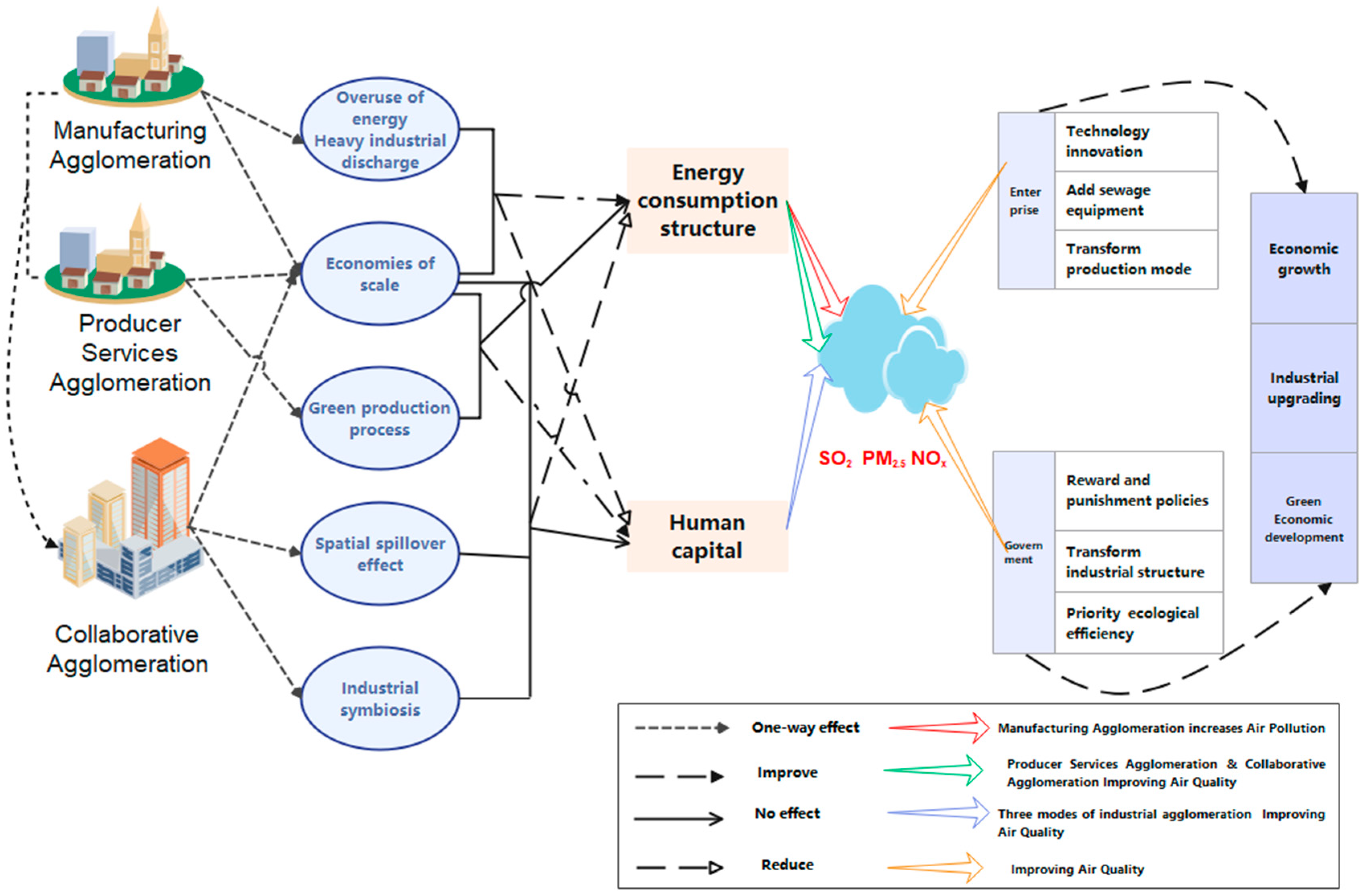
1.3.2. Theoretical Mechanisms
2. Data Sources
2.1. Setup of Econometric Model
2.2. Core variables
2.2.1. Explained Variables
2.2.2. Explanatory Variables
2.3. Mediating Variables and Control Variables
2.3.1. Mediating Variables
2.3.2. Control Variables
2.4. Data Sources
2.4.1. Data Sources
2.4.2. Descriptive Statistics of All Variables
3. Empirical Test
3.1. Baseline Regression
3.2. Heterogeneity Test
3.2.1. Regional Heterogeneity
3.2.2. Heterogeneity of Agglomeration
3.3. Robustness Test
3.3.1. First-Phase Lag
3.3.2. Spatial Correlation
- (1)
- Spatial correlation test
- (2)
- Regression results of spatial econometrics model
3.3.3. Instrumental Variables
3.4. Mechanism Test
3.4.1. Energy Consumption Structure
3.4.2. Human Capital
4. Result Discussion
4.1. Different Industrial Agglomeration Patterns
4.2. Heterogeneity
4.3. Mediating Mechanism Test
5. Conclusions and Suggestions
5.1. Research Summary
5.2. Policy Suggestions and Future Research
Author Contributions
Funding
Institutional Review Board Statement
Informed Consent Statement
Data Availability Statement
Conflicts of Interest
Abbreviation
| FGLS | Full Generalized Least Squares |
| OLS | Ordinary Least Square |
| GDP | Gross Domestic Product |
| R&D | Research and Development |
| QGIS | Quantum Geographic Information System |
| CPI | Consumer Price Index |
| FDI | Foreign Direct Investment |
| SDM | Spatial Dubin Model |
| 2SLS | Two-stage Least Squares |
Appendix A

| OLS+FE | FGLS | OLS+FE | FGLS | OLS+FE | FGLS | |
|---|---|---|---|---|---|---|
| PM2.5 | PM2.5 | NOx | NOx | SO2 | SO2 | |
| Magg | 6.663 * | 4.780 ** | 4.761 | 1.495 | 32.620 | 8.611 * |
| (3.408) | (1.982) | (9.551) | (4.061) | (19.587) | (4.699) | |
| ER | −3.108 | −1.688 | −16.746 | 9.114 | −2.979 | 1.016 |
| (13.368) | (7.409) | (52.828) | (15.500) | (61.016) | (22.041) | |
| RDintensity | −1.680 | −2.214 ** | −1.199 | −1.871 | −7.770 | −5.418 ** |
| (1.422) | (1.024) | (3.128) | (2.065) | (6.209) | (2.580) | |
| INS | −1.466 | 0.970 | 4.727 | −1.955 | 9.681 | 3.427 |
| (2.891) | (1.435) | (9.578) | (3.661) | (10.313) | (3.889) | |
| lnpergdp | 1.814 | 1.141 | 28.268 * | 15.128 *** | 44.008 * | 10.663 * |
| (4.265) | (2.261) | (15.566) | (5.739) | (21.700) | (6.238) | |
| fcp | −7.665 | −4.139 | −15.416 | −7.926 | −70.776 | −52.014 *** |
| (7.282) | (5.268) | (24.486) | (14.984) | (54.588) | (19.809) | |
| open | 0.623 | −1.122 | 29.499 ** | 16.009** | 2.031 | 5.308 |
| (4.800) | (2.641) | (13.831) | (7.067) | (21.618) | (7.636) | |
| city | −0.048 | −0.160 | −0.711 | 0.109 | −3.958*** | −1.832 *** |
| (0.360) | (0.149) | (0.610) | (0.344) | (0.800) | (0.406) | |
| _cons | 29.014 | 52.681** | −205.799 | −153.684 *** | −174.196 | 109.924 * |
| (32.894) | (20.885) | (132.732) | (53.896) | (193.941) | (60.640) | |
| N | 406 | 406 | 406 | 406 | 406 | 406.000 |
| R2 | 0.699 | 0.626 | 0.781 | |||
| time | Yes | Yes | Yes | Yes | Yes | Yes |
| ind | Yes | Yes | Yes |
References
- Qian, L.; Song, J.; Hao, H.; Wang, Y. Economic growth and pollutant emissions in China: A spatial econometric analysis. Stoch. Environ. Res. Risk Assess. 2014, 28, 429–442. [Google Scholar]
- He, C.; Huang, Z.; Ye, X. Spatial heterogeneity of economic development and industrial pollution in urban China. Stoch. Environ. Res. Risk Assess. 2014, 28, 767–781. [Google Scholar] [CrossRef]
- Zheng, X.; Yu, Y.; Wang, J.; Deng, H. Identifying the determinants and spatial nexus of provincial carbon intensity in china: A dynamic spatial panel approach. Reg. Environ. Change 2014, 14, 1651–1661. [Google Scholar] [CrossRef] [Green Version]
- Li, X.; Xu, Y.; Yao, X. Effects of industrial agglomeration on haze pollution: A Chinese city-level study. Energy Policy 2021, 148, 111928. [Google Scholar] [CrossRef]
- Cao, C.; Lee, X.; Liu, S.; Schultz, N.; Xiao, W.; Zhang, M.; Zhao, L. Urban heat islands in China enhanced by haze pollution. Nat. Commun. 2016, 7, 12509. [Google Scholar] [CrossRef]
- Yu, H.C.; Liu, Y.; Liu, C.L. Spatiotemporal variation and inequality in China’s economic resilience across cities and urban agglomerations. Sustainability 2018, 10, 4754. [Google Scholar] [CrossRef] [Green Version]
- Wang, S.; Jia, M.; Zhou, Y.; Fan, F. Impacts of changing urban form on ecological efficiency in China: A comparison between urban agglomerations and administrative areas. J. Environ. Plan. Manag 2019, 63, 1834–1856. [Google Scholar] [CrossRef]
- Fan, F.; Lian, H.; Liu, X.; Wang, X. Can environmental regulation promote urban green innovation efficiency? An empirical study based on Chinese cities. J. Clean. Prod 2020, 287, 125060. [Google Scholar] [CrossRef]
- Sun, C.Z.; Yan, X.D.; Zhao, L.S. Coupling efficiency measurement and spatial correlation characteristic of water-energy-food nexus in China. Resour. Conserv. Recycl. 2021, 164, 105151. [Google Scholar] [CrossRef]
- Chen, C.C.; Sun, Y.; Lan, Q.; Jiang, F. Impacts of industrial agglomeration on pollution and ecological efficiency-A spatial econometric analysis based on a big panel dataset of China’s 259 cities. J. Clean. Prod. 2020, 258, 120721. [Google Scholar] [CrossRef]
- Lu, W.; Tam, V.W.; Du, L.; Chen, H. Impact of industrial agglomeration on haze pollution: New evidence from Bohai Sea Economic Region in China. J. Clean. Prod. 2021, 280, 124414. [Google Scholar] [CrossRef]
- Liu, S.; Zhu, Y.; Du, K. The impact of industrial agglomeration on industrial pollutant emission: Evidence from China under New Normal. Clean Technol. Environ. Policy 2017, 19, 2327–2334. [Google Scholar] [CrossRef]
- Su, Y.; Yu, Y.Q. Spatial agglomeration of new energy industries on the performance of regional pollution control through spatial econometric analysis. Sci. Total Environ. 2020, 704, 135261. [Google Scholar] [CrossRef] [PubMed]
- Virkanen, J. Effect of urbanization on metal deposition in the bay of Töölönlahti, Southern Finland. Mar. Pollut. Bull 1998, 36, 729–738. [Google Scholar] [CrossRef]
- Frank, A. Urban air quality in larger conurbations in the European Union. Environ. Modell. Softw 2001, 16, 399–414. [Google Scholar]
- Markusen, J.R.; Venables, A.J. Foreign direct investment as a catalyst for industrial development. Eur. Econ. Rev 1999, 43, 335–356. [Google Scholar] [CrossRef] [Green Version]
- Shen, N.; Peng, H. Can industrial agglomeration achieve the emission-reduction effect? Socio-Econ. Plan. Sci. 2020, 75, 100867. [Google Scholar] [CrossRef]
- Peng, H.; Wang, Y.; Hu, Y.; Shen, H. Agglomeration production, industry association and carbon emission performance: Based on spatial analysis. Sustainability 2020, 12, 7234. [Google Scholar] [CrossRef]
- Li, X.; Zhu, X.; Li, J.; Gu, C. Influence of different industrial agglomeration modes on Eco-efficiency in China. Int. J. Environ. Res. Public Health 2021, 18, 13139. [Google Scholar] [CrossRef]
- Shen, N.; Zhao, Y.; Wang, Q. Diversified agglomeration, specialized agglomeration, and emission reduction effect—A Nonlinear Test Based on Chinese City Data. Sustainability 2018, 10, 2002. [Google Scholar] [CrossRef] [Green Version]
- Paci, R.; Usai, S. Externalities, knowledge spillovers and the spatial distribution of innovation. ERSA Conf. Pap. Eur. Reg. Sci. Assoc. 2000, 49, 381–390. [Google Scholar]
- Abdel-Rahman, H.; Fujita, M. Product variety, marshallian externalities, and city sizes. J. Reg. Sci. 1990, 30, 165–183. [Google Scholar] [CrossRef]
- Ma, R.; Wang, C.; Jin, Y.; Zhou, X. Estimating the effects of economic agglomeration on haze pollution in yangtze river delta china using an econometric analysis. Sustainability 2019, 11, 1893. [Google Scholar] [CrossRef] [Green Version]
- Hu, Z.; Cai, Y. Industrial agglomeration and industrial SO2 emissions in China’s 285 cities: Evidence from multiple agglomeration types. J. Clean. Prod. 2022, 353, 131675. [Google Scholar]
- Pei, Y.; Zhu, Y.; Liu, S.; Xie, M. Industrial agglomeration and environmental pollution: Based on the specialized and diversified agglomeration in the Yangtze River Delta. Environ. Dev. Sustain. 2020, 23, 4061–4085. [Google Scholar] [CrossRef]
- Cheng, Z. The spatial correlation and interaction between manufacturing agglomeration and environmental pollution. Ecol. Indic. 2016, 61, 1024–1032. [Google Scholar] [CrossRef]
- Zhu, Y.; Xia, Y. Industrial agglomeration and environmental pollution: Evidence from China under New Urbanization. Energy Environ. 2018, 30, 1010–1026. [Google Scholar] [CrossRef]
- Wu, J.; Xu, H.; Tang, K. Industrial agglomeration, CO2 emissions and regional development programs: A decomposition analysis based on 286 Chinese cities. Energy 2021, 225, 120239. [Google Scholar] [CrossRef]
- Selden, T.M.; Song, D. Environmental quality and development: Is there a Kuznets Curve for air pollution emissions? J. Environ. Econ. Manag. 1994, 27, 147–162. [Google Scholar] [CrossRef]
- Liu, J.; Qu, J.; Zhao, K. Is China’s development conforms to the Environmental Kuznets Curve hypothesis and the pollution haven hypothesis? J. Clean. Prod. 2019, 234, 787–796. [Google Scholar] [CrossRef]
- Cansino, J.M.; Román-Collado, R.; Molina, J.C. Quality of institutions, technological progress, and pollution havens in Latin America. An analysis of the Environmental Kuznets Curve hypothesis. Sustainability 2019, 11, 3708. [Google Scholar] [CrossRef] [Green Version]
- Sarkodie, S.A.; Strezov, V. Effect of foreign direct investments, economic development and energy consumption on greenhouse gas emissions in developing countries. Sci. Total Environ. 2019, 646, 862–871. [Google Scholar] [CrossRef] [PubMed]
- Gill, A.R.; Viswanathan, K.K.; Hassan, S. The Environmental Kuznets Curve (EKC) and the environmental problem of the day. Renew. Sust. Energ. Rev. 2018, 81, 1636–1642. [Google Scholar] [CrossRef]
- List, J.A.; Catherine, Y.C. The effects of environmental regulations on foreign direct investment. J. Environ. Econ. Manag. 2000, 40, 1–20. [Google Scholar] [CrossRef] [Green Version]
- AI-Mulali, U.; Weng-Wai, C.; Sheau-Ting, L.; Mohammed, A.H. Investigating the environmental Kuznets curve (EKC) hypothesis by utilizing the ecological footprint as an indicator of environmental degradation. Ecol. Indic 2015, 48, 315–323. [Google Scholar] [CrossRef]
- Jie, H. Pollution haven hypothesis and environmental impacts offoreign direct investment: The case of industrial emission of sulfur dioxide (SO2) in Chinese provinces. Ecol. Econ 2006, 60, 228–245. [Google Scholar]
- Baomin, D.; Jiong, G.; Xin, Z. FDI and environmental regulation: Pollution haven or a race to the top? J. Regul. Econ 2012, 41, 216–237. [Google Scholar]
- Kheder, S.B.; Zugravu, N. Environmental regulation and French firms location abroad: An economic geography model in an international comparative study. Ecol. Econ 2012, 77, 48–61. [Google Scholar] [CrossRef]
- Baldwin, J.R.; Brown, W.M.; Rigby, D.L. Agglomeration economics: Microdata panel estimates from Canadian manufacturing. J. Reg. Sci 2010, 50, 915–934. [Google Scholar] [CrossRef]
- Drucker, J.; Feser, E. Regional industrial structure and agglomeration economies: An analysis of productivity in three manufacturing industries. Reg. Sci. Urban Econ 2012, 42, 1–14. [Google Scholar] [CrossRef]
- Ye, P.; Xia, S.; Xiong, Y.; Liu, C.; Li, F.; Liang, J.; Zhang, H. Did an ultra-low emissions policy on coal-fueled thermal power reduce the harmful emissions? Evidence from three typical air pollutants abatement in China. Int. J. Environ. Res. Public Health 2020, 17, 8555. [Google Scholar] [CrossRef] [PubMed]
- Zhou, X.; Feng, C. The impact of environmental regulation on fossil energy consumption in China: Direct and indirect effects. J. Clean. Prod. 2017, 142, 3174–3183. [Google Scholar] [CrossRef]
- Hao, Y.; Song, J.; Shen, Z. Does industrial agglomeration affect the regional environment? Evidence from Chinese cities. Environ. Sci. Pollut. Res. 2021, 29, 7811–7826. [Google Scholar] [CrossRef] [PubMed]
- Verhoef, E.T.; Nijkamp, P. Externalities in urban sustainability: Environmental versus localization-type agglomeration externalities in a general spatial equilibrium model of a single-sector monocentric industrial city. Ecol. Econ 2002, 40, 157–179. [Google Scholar] [CrossRef] [Green Version]
- Zhu, Y.; Du, W.; Zhang, J. Does industrial collaborative agglomeration improve environmental efficiency? Insights from China’s population structure. Environ. Sci. Pollut. Res. 2021, 29, 5072–5091. [Google Scholar] [CrossRef]
- Thiel, C.; Nijs, W.; Simoes, S.; Schmidt, J.; Zyl, A.V.; Schmid, E. The impact of the EU car CO2 regulation on the energy system and the role of electro-mobility to achieve transport decarbonisation. Energy Policy 2016, 96, 153–166. [Google Scholar] [CrossRef]
- Ehrlich, P.R.; Holdren, J.R. Impact of population growth. Science 1971, 171, 1212–1217. [Google Scholar] [CrossRef]
- Dietz, T.; Rosa, E.A. Rethinking the environmental impacts of population, Afflfluence and technology. Hum. Ecol. Rev. 1994, 2, 277–300. [Google Scholar]
- Wooldridge, J.M. Introductory Econometrics: A Modern Approach; Cengage Learn: Boston, MA, USA, 2015. [Google Scholar]
- Meyer, D.; Riechert, M. Open source QGIS toolkit for the Advanced Research WRF modelling system. Environ. Modell. Softw 2019, 112, 166–178. [Google Scholar] [CrossRef] [Green Version]
- Gallardo-Salazar, J.L.; Rosas-Chavoya, M. Dissemination of free and open source geospatial software a case QGIS Mexico. Rev. Geogr. Venez. 2021, 62, 532–543. [Google Scholar]
- Graser, A.; Olaya, V. Processing: A Python Framework for the Seamless Integration of Geoprocessing Tools in QGIS. ISPRS Int. Geo-Inf. 2015, 4, 2219–2245. [Google Scholar] [CrossRef]
- Oxoli, D.; Prestifilippo, G.; Bertocchi, D.; Zurbaran, M. Enabling spatial autocorrelation mapping in QGIS: The Hotspot Analysis Plugin. Geam-Geoint. Ambient. Min. 2017, 45–50. [Google Scholar]
- Park, S.; Nielsen, A.; Bailey, R.T.; Trolle, D.; Bieger, K. A QGIS-based graphical user interface for application and evaluation of SWAT-MODFLOW models. Environ. Modell. Softw 2019, 111, 493–497. [Google Scholar] [CrossRef]
- Sebbah, B.; Alaoui, O.Y.; Wahbi, M.; Maatouk, M.; Ben Achhab, N. QGIS-Landsat Indices plugin (Q-LIP): Tool for environmental indices computing using Landsat data. Environ. Modell. Softw 2021, 137, 5. [Google Scholar] [CrossRef]
- Donoghue, D.; Gleave, B. A note on methods for measuring industrial agglomeration. Reg. Stud. 2004, 38, 419–427. [Google Scholar] [CrossRef]
- Glaesere. The spatial economy: Cities. regions. and international trade. J. Econ. 1962, 73, 111–123. [Google Scholar]
- Martin, P.; Mayer, T.; Mayneris, F. Spatial Concentration and Plant—Level Productivity in France. J. Urban Econ. 2011, 69, 182–195. [Google Scholar] [CrossRef] [Green Version]
- Li, G.; Fang, X.; Liu, M. Environmental governance effect of the transformation of export trade mode: Empirical evidence from 194 cities in China. Environ. Sci. Pollut. Res. 2022, 29, 22756–22770. [Google Scholar] [CrossRef]
- Zhao, Q. Does state-owned enterprise really ineffificient? Based on the perspective of regional innovation effificiency spillover effect. Sci. Sci. Manag. 2017, 38, 107–116. [Google Scholar]
- Anselin, L. Spatial Econometrics: Methods and Models; Springer Science & Business Media: Berlin/Heidelberg, Germany, 1988. [Google Scholar]
- Elhorst, J.P. Matlab software for spatial panels. Int. Reg. Sci. Rev. 2014, 37, 389–405. [Google Scholar] [CrossRef] [Green Version]
- Combes, P.P.; Overman, H.G. The spatial distribution of economic activities in the European Union. Handb. Reg. Urban Econ. 2004, 4, 2845–2909. [Google Scholar]
- Dell, M. The Persistent Effects of Peru’s Mining Mita. Econometrica 2010, 78, 1863–1903. [Google Scholar] [CrossRef] [Green Version]
- Baron, R.M.; Kenny, D.A. The moderator–mediator variable distinction in social psychological research: Conceptual, strategic, and statistical considerations. J. Pers. Soc. Psychol. 1986, 51, 1173. [Google Scholar] [CrossRef] [PubMed]
- Gonzalez, O.; Mackinnon, D.P. A Bifactor Approach to Model Multifaceted Constructs in Statistical Mediation Analysis. Educ. Psychol. Meas 2016, 78, 5–31. [Google Scholar] [CrossRef]
- Shao, W.; Yin, Y.; Bai, X.; Taghizadeh-Hesary, F. Analysis of the Upgrading Effect of the Industrial Structure of Environmental Regulation: Evidence From 113 Cities in China. Front. Environ. Sci. 2021, 9, 232. [Google Scholar] [CrossRef]
- Ellison, G.; Glaeser, E.L. The geographic concentration of industry: Does natural advantage explain agglomeration? Am. Econ. Rev. 1999, 89, 311–316. [Google Scholar] [CrossRef] [Green Version]
- Kyriakopoulou, E.; Xepapadeas, A. First nature advantage and the emergence of economic clusters. Reg. Sci. Urban. Econ. 2013, 43, 101–116. [Google Scholar] [CrossRef]
- Chen, H.X.; Li, G.P. Empirical study on effect of industrial structure change on regional economic growth of Beijing-Tianjin-Hebei Metropolitan Region. Chin. Geogr. Sci. 2011, 21, 708–714. [Google Scholar] [CrossRef]
- Liang, G.F.; Yu, D.J.; Ke, L.F. An Empirical Study on Dynamic Evolution of Industrial Structure and Green Economic Growth-Based on Data from China’s Underdeveloped Areas. Sustainability 2021, 13, 8154. [Google Scholar] [CrossRef]
- Chen, M.Q. A study of low-carbon development, urban innovation and industrial structure upgrading in China. Int. J. Low-Carbon Technol. 2022, 17, 185–195. [Google Scholar] [CrossRef]
- Khanum, F.; Chaudhry, M.N.; Kumar, P. Characterization of five-year observation data of fine particulate matter in the metropolitan area of Lahore. Air Qual. Atmos. Health 2017, 10, 725–736. [Google Scholar] [CrossRef] [PubMed] [Green Version]
- Li, J.; Reiffs, A.; Parchatka, U.; Fischer, H. In Situ Measurements of Atmospheric CO and Its Correlation with Nox And O3 at a Rural Mountain Site. Metrol. Meas. Syst. 2015, 22, 25–38. [Google Scholar] [CrossRef]


| Variable Type | Variable Name | Indicators | Data Source |
|---|---|---|---|
| Explained variables | PM2.5 | Annual average PM2.5 concentration | China Environmental Yearbook |
| SO2 | Average annual emissions (ten thousand tons) | ||
| NOx | Average annual emissions (ten thousand tons) | ||
| Core explanatory variables | Manufacturing agglomeration | % | Statistical Yearbook of Chinese Provinces |
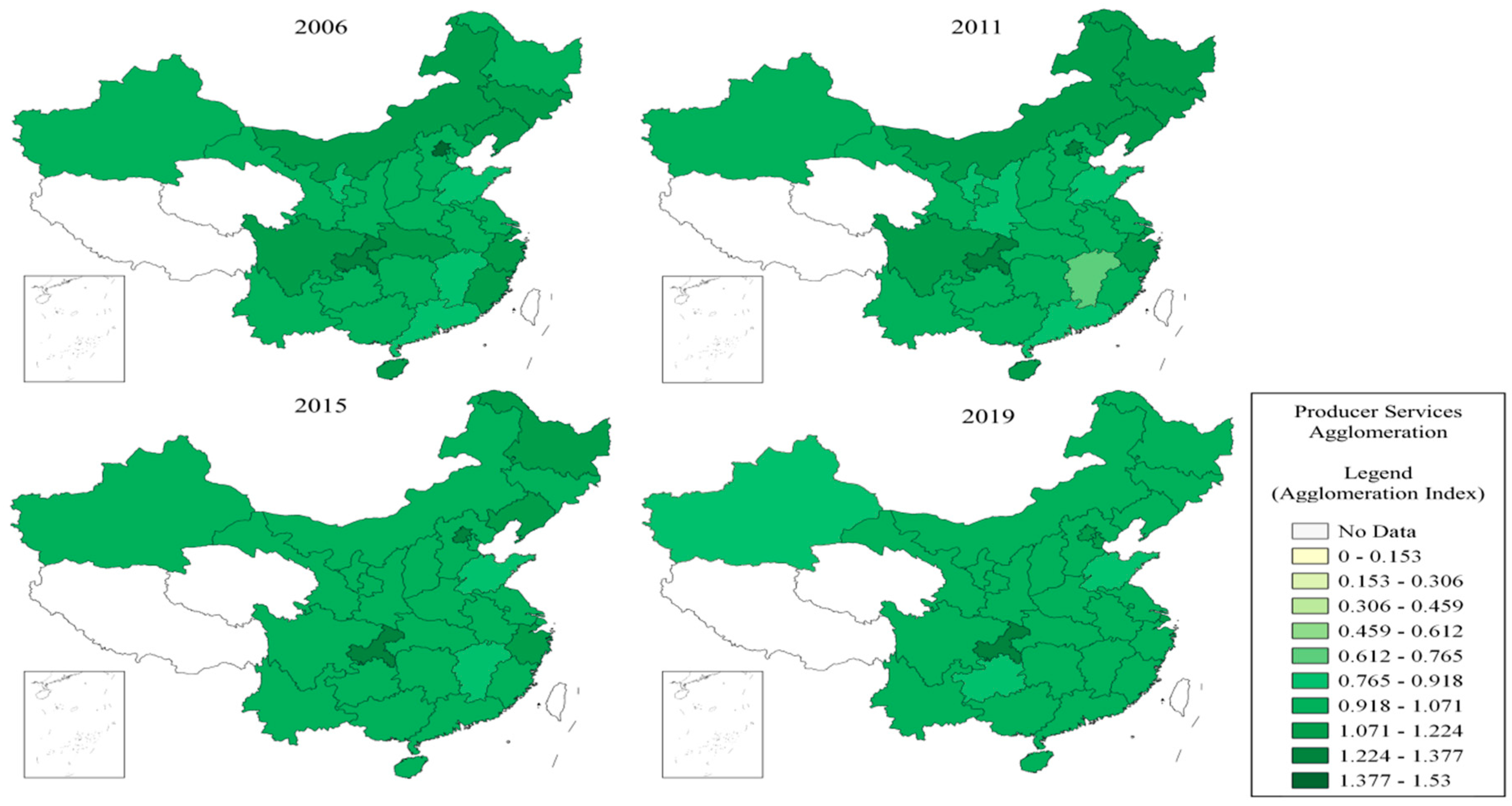
| Producer services agglomeration | % | ||
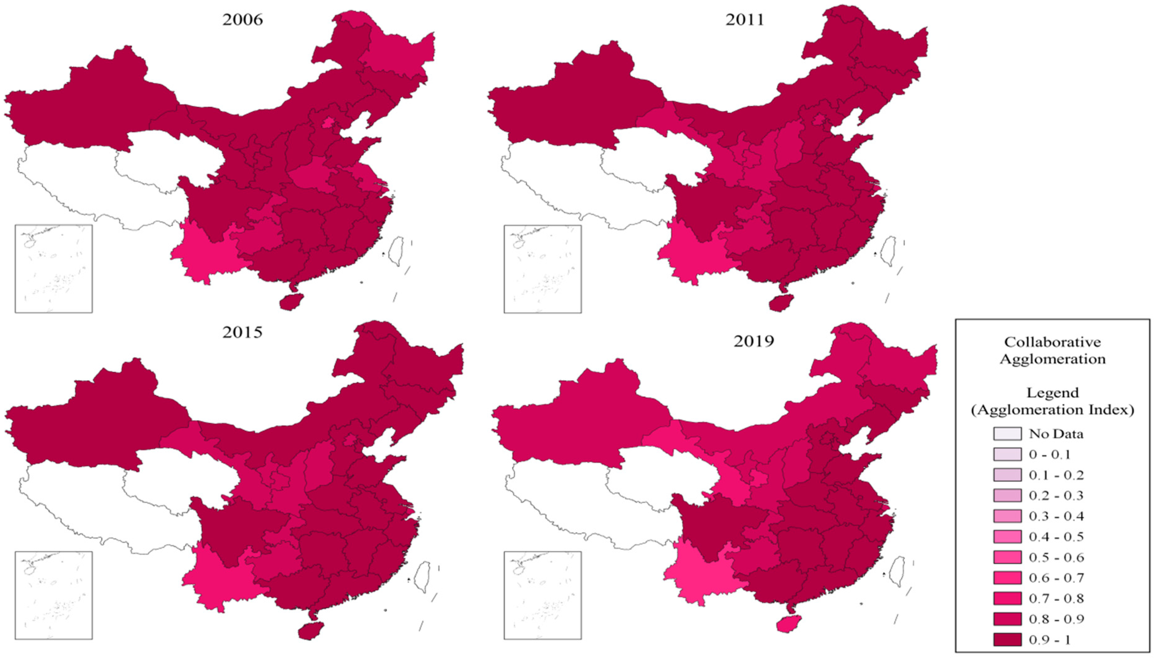
| Collaborative agglomeration | % | ||
| Intermediate variables | Energy consumption structure | Ratio of coal consumption to total energy consumption | China Energy Statistical Yearbook |
| Human capital | Ratio of R&D personnel to total employees | China Statistical Yearbook | |
| Control variables | Environmental regulation | Proportion of pollution control | China Environmental Statistics Yearbook & China Statistical Yearbook |
| R&D intensity | R&D investment intensity | China Statistical Yearbook of Science and Technology | |
| Industrial structure | Proportion of secondary industry in tertiary industry | CSMAR | |
| GDP per capita | Real GDP per capita | China Statistical Yearbook | |
| GDP per capita squared | Real GDP per capita squared | ||
| FDI stock | Share of FDI stock in GDP | ||
| Open | Foreign trade dependence | CSMAR | |
| City | Proportion of urban population | NOAA/NGDC |
| Variable | Obs | Mean | Std. Dev. | Min | Max | Unit |
|---|---|---|---|---|---|---|
| Magg | 406 | 1.104 | 0.213 | 0.723 | 2.040 | % |
| Sagg | 406 | 1.024 | 0.110 | 0.756 | 1.528 | % |
| Cagg | 406 | 0.916 | 0.071 | 0.637 | 0.999 | % |
| SO2 | 406 | 59.810 | 43.940 | 0.190 | 196.200 | ten thousand tons |
| NOx | 406 | 59.555 | 39.034 | 4.000 | 180.113 | ten thousand tons |
| PM2.5 | 406 | 42.522 | 13.807 | 16.090 | 85.628 | µg/m3 |
| ER | 406 | 0.011 | 0.014 | 0.001 | 0.224 | % |
| RDintensity | 406 | 1.575 | 1.093 | 0.200 | 6.310 | % |
| INS | 406 | 1.096 | 0.356 | 0.193 | 2.001 | % |
| lnpergdp | 406 | 10.314 | 0.557 | 8.646 | 11.685 | Yuan |
| lnpergdp2 | 406 | 106.708 | 11.487 | 74.760 | 136.540 | % |
| fcp | 406 | 0.178 | 0.136 | 0.005 | 0.672 | % |
| open | 406 | 0.295 | 0.324 | 0.028 | 1.668 | % |
| city | 406 | 54.863 | 13.724 | 27.460 | 89.600 | % |
| Energy | 406 | 0.963 | 0.421 | −0.591 | 2.460 | % |
| RDhuman | 406 | 0.012 | 0.008 | 0.000 | 0.054 | % |
| OLS+FE | FGLS | OLS+FE | FGLS | OLS+FE | FGLS | |
|---|---|---|---|---|---|---|
| PM2.5 | PM2.5 | NOx | NOx | SO2 | SO2 | |
| Magg | 6.985 ** | 4.588 ** | 4.899 | 1.384 | 33.033 * | 7.992 * |
| (3.106) | (1.984) | (9.608) | (4.035) | (19.226) | (4.680) | |
| ER | −0.624 | −1.860 | −15.680 | 9.303 | 0.208 | −0.589 |
| (13.147) | (7.507) | (52.543) | (15.663) | (57.342) | (22.277) | |
| RDintensity | −0.132 | −1.063 | −0.534 | −0.306 | −5.784 | −4.097 |
| (1.404) | (1.141) | (3.620) | (2.168) | (5.301) | (2.693) | |
| INS | −1.610 | 1.030 | 4.665 | −2.721 | 9.496 | 2.628 |
| (2.659) | (1.467) | (9.664) | (3.655) | (10.379) | (3.899) | |
| lnpergdp | 80.641 ** | 43.103 ** | 62.118 | 145.871 ** | 145.149 | 143.477 ** |
| (36.389) | (17.992) | (103.261) | (59.627) | (227.332) | (70.027) | |
| lnpergdp2 | −3.948 ** | −2.133 ** | −1.695 | −6.394 ** | −5.065 | −6.565 * |
| (1.855) | (0.897) | (4.972) | (2.899) | (10.842) | (3.435) | |
| fcp | −16.433 | −10.172* | −19.181 | −22.876 | −82.026 | −71.732 *** |
| (9.699) | (5.892) | (26.063) | (16.281) | (55.893) | (22.241) | |
| open | −2.849 | −2.806 | 28.008* | 9.245 | −2.425 | 0.160 |
| (4.526) | (2.767) | (14.797) | (7.698) | (27.561) | (8.119) | |
| city | −0.151 | −0.148 | −0.755 | −0.092 | −4.090 *** | −1.948 *** |
| (0.295) | (0.150) | (0.649) | (0.355) | (0.837) | (0.410) | |
| _cons | −357.061 * | −149.091 * | −371.588 | −785.371 *** | −669.565 | −530.539 |
| (179.709) | (87.636) | (526.066) | (291.978) | (1164.765) | (343.105) | |
| N | 406 | 406 | 406 | 406 | 406 | 406 |
| R2 | 0.714 | 0.626 | 0.782 | |||
| time | Yes | Yes | Yes | Yes | Yes | Yes |
| ind | Yes | Yes | Yes |
| OLS+FE | FGLS | OLS+FE | FGLS | OLS+FE | FGLS | |
|---|---|---|---|---|---|---|
| PM2.5 | PM2.5 | NOx | NOx | SO2 | SO2 | |
| Sagg | −5.632 | −9.140 ** | 27.469 | 14.527 * | 11.314 | −1.011 |
| (8.697) | (4.036) | (19.654) | (8.555) | (44.863) | (10.052) | |
| ER | 1.400 | −1.265 | −19.389 | 7.955 | 3.584 | −1.687 |
| (12.827) | (7.519) | (56.295) | (15.339) | (63.058) | (22.339) | |
| RDintensity | −0.387 | −0.891 | −2.681 | −0.602 | −9.366 | −3.783 |
| (1.783) | (1.146) | (4.070) | (2.137) | (6.241) | (2.694) | |
| INS | −1.514 | 1.179 | 7.108 | −2.331 | 12.821 | 2.715 |
| (2.651) | (1.478) | (9.652) | (3.577) | (11.385) | (3.922) | |
| lnpergdp | 81.902 ** | 46.780 ** | 37.861 | 139.458 ** | 120.747 | 147.614 ** |
| (38.966) | (18.469) | (102.611) | (59.143) | (240.403) | (70.425) | |
| lnpergdp2 | −4.082 ** | −2.359 ** | −0.582 | −6.080 ** | −4.241 | −6.855 ** |
| (1.948) | (0.920) | (5.026) | (2.877) | (11.486) | (3.452) | |
| fcp | −17.486 * | −10.144 * | −22.080 | −22.395 | −89.614 | −71.197 *** |
| (9.963) | (6.016) | (25.679) | (16.256) | (60.963) | (22.172) | |
| open | −2.788 | −3.096 | 28.806* | 9.346 | −1.222 | 0.237 |
| (4.690) | (2.820) | (15.143) | (7.627) | (28.468) | (8.118) | |
| city | −0.087 | −0.070 | −0.850 | −0.151 | −3.955 *** | −1.891 *** |
| (0.306) | (0.153) | (0.619) | (0.349) | (0.896) | (0.412) | |
| _cons | −346.198 * | −154.554 * | −260.854 | −763.354 *** | −493.653 | −539.332 |
| (197.327) | (89.571) | (510.347) | (288.618) | (1225.996) | (345.034) | |
| N | 406 | 406 | 406 | 406 | 406 | 406 |
| R2 | 0.709 | 0.630 | 0.776 | |||
| time | Yes | Yes | Yes | Yes | Yes | Yes |
| ind | Yes | Yes | Yes |
| OLS+FE | FGLS | OLS+FE | FGLS | OLS+FE | FGLS | |
|---|---|---|---|---|---|---|
| PM2.5 | PM2.5 | NOx | NOx | SO2 | SO2 | |
| Cagg | −14.455 * | −9.071** | 9.694 | −0.952 | −32.474 | −5.527 |
| (7.305) | (4.538) | (28.569) | (10.422) | (54.422) | (11.594) | |
| ER | −0.301 | −1.592 | −14.381 | 9.344 | 3.676 | −1.378 |
| (12.894) | (7.350) | (53.591) | (15.685) | (59.568) | (22.148) | |
| RDintensity | −0.623 | −1.138 | −1.039 | −0.333 | −8.395 | −3.657 |
| (1.377) | (1.139) | (3.845) | (2.184) | (6.763) | (2.675) | |
| INS | −0.784 | 1.294 | 4.827 | −2.728 | 12.649 | 2.722 |
| (2.797) | (1.478) | (9.566) | (3.657) | (11.345) | (3.946) | |
| lnpergdp | 62.974 * | 34.472 * | 69.513 | 144.021 ** | 97.403 | 143.424 ** |
| (33.439) | (18.272) | (102.361) | (60.584) | (241.959) | (71.386) | |
| lnpergdp2 | −3.124 * | −1.753 * | −2.135 | −6.312 ** | −3.010 | −6.669 * |
| (1.665) | (0.914) | (4.890) | (2.949) | (11.592) | (3.501) | |
| fcp | −14.466 | −10.166* | −22.476 | −23.192 | −81.182 | −70.156 *** |
| (9.298) | (5.991) | (28.146) | (16.431) | (60.544) | (22.300) | |
| open | −2.476 | −2.155 | 28.028* | 9.624 | −1.098 | −0.088 |
| (4.796) | (2.796) | (14.499) | (7.719) | (28.720) | (8.150) | |
| city | −0.150 | −0.103 | −0.702 | −0.075 | −3.990*** | −1.872 *** |
| (0.269) | (0.149) | (0.653) | (0.353) | (0.950) | (0.414) | |
| _cons | −243.949 | −92.953 | −407.181 | −774.714 *** | −342.603 | −514.180 |
| (169.460) | (89.177) | (523.263) | (298.283) | (1261.598) | (351.630) | |
| N | 406 | 406 | 406 | 406 | 406 | 406 |
| R2 | 0.714 | 0.626 | 0.777 | |||
| time | Yes | Yes | Yes | Yes | Yes | Yes |
| ind | Yes | Yes | Yes |
| Eastern China | Central and Western China | Eastern China | Central and Western China | Eastern China | Central and Western China | |
|---|---|---|---|---|---|---|
| PM2.5 | PM2.5 | NOx | NOx | SO2 | SO2 | |
| Magg | 1.352 | 6.208 *** | 1.683 | −0.369 | 22.176 ** | 6.461 |
| (3.290) | (2.269) | (5.525) | (6.670) | (9.396) | (5.964) | |
| Sagg | −9.249 | −12.662 *** | −13.010 | 21.519 ** | −38.008 * | 4.796 |
| (7.555) | (4.107) | (18.336) | (10.820) | (23.065) | (11.601) | |
| Cagg | −1.105 | −11.606 ** | 6.016 | 12.151 | 17.978 | −19.301 |
| (8.484) | (4.931) | (14.671) | (15.745) | (22.713) | (13.892) | |
| Control | Yes | Yes | Yes | Yes | Yes | Yes |
| time | Yes | Yes | Yes | Yes | Yes | Yes |
| ind | Yes | Yes | Yes | Yes | Yes | Yes |
| N | 168 | 238 | 168 | 238 | 168 | 238 |
| Eastern China | Central and Western China | Eastern China | Central and Western China | Eastern China | Central and Western China | |
|---|---|---|---|---|---|---|
| PM2.5 | PM2.5 | NOx | NOx | SO2 | SO2 | |
| Mrdi | 37.159 *** | 15.127 *** | 79.980 *** | 1.103 | 33.075 ** | −11.532 * |
| (5.687) | (3.463) | (14.082) | (7.377) | (15.768) | (6.516) | |
| Mcom | −14.525 *** | −5.198 *** | −31.503 *** | 1.637 | −13.976 ** | 2.712 |
| (2.388) | (1.425) | (6.134) | (3.096) | (6.774) | (2.808) | |
| Srdi | 17.280 ** | 3.166 | 6.873 | −1.157 | 9.418 | −0.903 |
| (7.705) | (4.111) | (19.117) | (7.142) | (13.550) | (6.787) | |
| Scom | −57.070 *** | −0.243 | −116.603 *** | 4.265 | −79.167 *** | −6.355 |
| (10.738) | (3.275) | (30.536) | (7.807) | (27.396) | (6.580) | |
| Control | Yes | Yes | Yes | Yes | Yes | Yes |
| time | Yes | Yes | Yes | Yes | Yes | Yes |
| ind | Yes | Yes | Yes | Yes | Yes | Yes |
| N | 168 | 238 | 168 | 238 | 168 | 238 |
| (1) | (2) | (3) | |
|---|---|---|---|
| SO2 | NOx | PM2.5 | |
| LMagg | 5.092 | 5.447 | 5.256 ** |
| (5.188) | (4.084) | (2.135) | |
| LSagg | −2.934 | 3.301 | −7.342 * |
| (10.706) | (8.960) | (4.111) | |
| LCagg | 3.364 | −2.642 | −9.517 ** |
| (12.817) | (10.719) | (4.750) | |
| Control | Yes | Yes | Yes |
| time | Yes | Yes | Yes |
| ind | Yes | Yes | Yes |
| N | 377 | 377 | 377 |
| Year | PM2.5 | NOx | SO2 | |||
|---|---|---|---|---|---|---|
| Moran’I | p-Value | Moran’I | p-Value | Moran’I | p-Value | |
| 2006 | 0.135 | 0.000 | 0.032 | 0.050 | −0.015 | 0.562 |
| 2007 | 0.128 | 0.000 | −0.015 | 0.565 | −0.016 | 0.581 |
| 2008 | 0.120 | 0.000 | 0.011 | 0.174 | −0.016 | 0.580 |
| 2009 | 0.135 | 0.000 | 0.010 | 0.181 | −0.017 | 0.590 |
| 2010 | 0.140 | 0.000 | 0.010 | 0.185 | −0.017 | 0.588 |
| 2011 | 0.118 | 0.000 | 0.029 | 0.059 | 0.011 | 0.167 |
| 2012 | 0.091 | 0.000 | 0.028 | 0.063 | 0.011 | 0.171 |
| 2013 | 0.121 | 0.000 | 0.026 | 0.070 | 0.012 | 0.158 |
| 2014 | 0.143 | 0.000 | 0.025 | 0.074 | 0.011 | 0.170 |
| 2015 | 0.155 | 0.000 | 0.023 | 0.084 | 0.011 | 0.169 |
| 2016 | 0.147 | 0.000 | −0.012 | 0.484 | −0.014 | 0.539 |
| 2017 | 0.134 | 0.000 | −0.009 | 0.427 | −0.032 | 0.915 |
| 2018 | 0.120 | 0.000 | 0.001 | 0.280 | −0.034 | 0.978 |
| 2019 | 0.112 | 0.000 | −0.001 | 0.313 | −0.035 | 0.991 |
| (1) | (2) | (3) | |
|---|---|---|---|
| SDM | SDM | SDM | |
| Magg | 6.445 ** | ||
| (3.036) | |||
| Sagg | −8.595 * | ||
| (5.010) | |||
| Cagg | −13.92 ** | ||
| (7.099) | |||
| ER | 2.256 | 4.332 | 1.196 |
| (15.10) | (9.726) | (14.73) | |
| RDintensity | 0.471 | −0.672 | −0.218 |
| (1.381) | (1.738) | (1.292) | |
| INS | −5.775 ** | −0.654 | −5.188 * |
| (2.550) | (2.238) | (2.914) | |
| lnpergdp | 124.9 *** | 75.70 ** | 112.3 *** |
| (36.77) | (35.71) | (35.40) | |
| lnpergdp2 | −6.064 *** | −3.832 ** | −5.458 *** |
| (1.771) | (1.749) | (1.678) | |
| fcp | −20.69 ** | −20.93 ** | −18.92 ** |
| (8.800) | (9.510) | (8.603) | |
| open | −9.397 * | −1.656 | −9.093 * |
| (4.802) | (4.628) | (5.106) | |
| city | −0.0431 | 0.0398 | −0.0432 |
| (0.221) | (0.241) | (0.206) |
| (1) | (2) | (3) | (4) | (5) | (6) | (7) | (8) | (9) | |
|---|---|---|---|---|---|---|---|---|---|
| PM2.5 | NOx | SO2 | PM2.5 | NOx | SO2 | PM2.5 | NOx | SO2 | |
| Magg | 152.499 * | 158.487 | −56.902 | ||||||
| (79.780) | (108.735) | (130.843) | |||||||
| Sagg | −188.565 ** | −195.969 | 70.360 | ||||||
| (74.064) | (122.180) | (161.078) | |||||||
| Cagg | −579.759 *** | −609.259 ** | −175.468 | ||||||
| (189.101) | (260.072) | (162.490) | |||||||
| Control | Yes | Yes | Yes | Yes | Yes | Yes | Yes | Yes | Yes |
| time | Yes | Yes | Yes | Yes | Yes | Yes | Yes | Yes | Yes |
| ind | Yes | Yes | Yes | Yes | Yes | Yes | Yes | Yes | Yes |
| N | 406 | 406 | 406 | 406 | 406 | 406 | 406 | 406 | 406 |
| (1) | (2) | (3) | (4) | |
|---|---|---|---|---|
| Energy | PM2.5 | NOx | SO2 | |
| Magg | 0.249 * | 5.805 * | 6.928 | 34.766 * |
| (0.128) | (2.968) | (9.771) | (18.511) | |
| Energy | 4.740* | −8.147 | −6.956 | |
| (2.563) | (6.426) | (13.944) | ||
| Control | Yes | Yes | Yes | Yes |
| time | Yes | Yes | Yes | Yes |
| ind | Yes | Yes | Yes | Yes |
| N | 406 | 406 | 406 | 406 |
| (1) | (2) | (3) | (4) | |
|---|---|---|---|---|
| Energy | PM2.5 | NOx | SO2 | |
| Sagg | 0.227 | −6.863 | 29.356 | 12.274 |
| (0.288) | (8.529) | (19.086) | (44.597) | |
| Energy | 5.434 * | −8.332 | −4.239 | |
| (2.673) | (6.039) | (14.744) | ||
| Control | Yes | Yes | Yes | Yes |
| time | Yes | Yes | Yes | Yes |
| ind | Yes | Yes | Yes | Yes |
| N | 406 | 406 | 406 | 406 |
| (1) | (2) | (3) | (4) | |
|---|---|---|---|---|
| Energy | PM2.5 | NOx | SO2 | |
| Cagg | −1.078 *** | −9.613 | 1.712 | −40.089 |
| (0.275) | (6.952) | (30.476) | (56.803) | |
| Energy | 4.492 * | −7.405 | −7.064 | |
| (2.583) | (6.764) | (15.187) | ||
| Control | Yes | Yes | Yes | Yes |
| time | Yes | Yes | Yes | Yes |
| ind | Yes | Yes | Yes | Yes |
| N | 406 | 406 | 406 | 406 |
| (1) | (2) | (3) | (4) | |
|---|---|---|---|---|
| RDhuman | PM2.5 | NOx | SO2 | |
| Magg | −0.002 * | 3.862 ** | 1.316 | 7.518 |
| (0.001) | (1.939) | (4.063) | (4.694) | |
| RDhuman | −170.193 *** | −193.257 | −65.690 | |
| (57.486) | (156.454) | (143.192) | ||
| Control | Yes | Yes | Yes | Yes |
| time | Yes | Yes | Yes | Yes |
| ind | Yes | Yes | Yes | Yes |
| N | 406 | 406 | 406 | 406 |
| (1) | (2) | (3) | (4) | |
|---|---|---|---|---|
| RDhuman | PM2.5 | NOx | SO2 | |
| Sagg | 0.005 ** | −8.478 ** | 15.267 * | −2.180 |
| (0.002) | (3.948) | (8.592) | (10.210) | |
| RDhuman | −176.616 *** | −202.163 | −64.309 | |
| (56.690) | (155.538) | (144.712) | ||
| Control | Yes | Yes | Yes | Yes |
| time | Yes | Yes | Yes | Yes |
| ind | Yes | Yes | Yes | Yes |
| N | 406 | 406 | 406 | 406 |
| (1) | (2) | (3) | (4) | |
|---|---|---|---|---|
| RDhuman | PM2.5 | NOx | SO2 | |
| Cagg | 0.004 | −8.843 ** | −0.402 | −4.277 |
| (0.003) | (4.438) | (10.494) | (11.607) | |
| RDhuman | −175.759 *** | −193.447 | −65.051 | |
| (57.768) | (156.631) | (143.488) | ||
| Control | Yes | Yes | Yes | Yes |
| time | Yes | Yes | Yes | Yes |
| ind | Yes | Yes | Yes | Yes |
| N | 406 | 406 | 406 | 406 |
Publisher’s Note: MDPI stays neutral with regard to jurisdictional claims in published maps and institutional affiliations. |
© 2022 by the authors. Licensee MDPI, Basel, Switzerland. This article is an open access article distributed under the terms and conditions of the Creative Commons Attribution (CC BY) license (https://creativecommons.org/licenses/by/4.0/).
Share and Cite
Ye, P.; Li, J.; Ma, W.; Zhang, H. Impact of Collaborative Agglomeration of Manufacturing and Producer Services on Air Quality: Evidence from the Emission Reduction of PM2.5, NOx and SO2 in China. Atmosphere 2022, 13, 966. https://doi.org/10.3390/atmos13060966
Ye P, Li J, Ma W, Zhang H. Impact of Collaborative Agglomeration of Manufacturing and Producer Services on Air Quality: Evidence from the Emission Reduction of PM2.5, NOx and SO2 in China. Atmosphere. 2022; 13(6):966. https://doi.org/10.3390/atmos13060966
Chicago/Turabian StyleYe, Penghao, Jin Li, Wenjing Ma, and Huarong Zhang. 2022. "Impact of Collaborative Agglomeration of Manufacturing and Producer Services on Air Quality: Evidence from the Emission Reduction of PM2.5, NOx and SO2 in China" Atmosphere 13, no. 6: 966. https://doi.org/10.3390/atmos13060966