
Climatological Study of Ozone over Saudi Arabia
by
 , , and
Saleha Al-Kallas
1, 
Motirh Al-Mutairi
1,
Heshmat Abdel Basset
2,
Abdallah Abdeldym
2,*,
Mostafa Morsy
2 and
Ayman Badawy
3 1
Faculty of Arts, Princess Nourah Bint Abdulrahman University, Riyadh 11671, Saudi Arabia
2
Department of Astronomy and Meteorology, Faculty of Science, Al-Azhar University, Cairo 11884, Egypt
3
Egyptian Meteorological Authority, Cairo 11784, Egypt
*
Author to whom correspondence should be addressed.
Atmosphere 2021, 12(10), 1275; https://doi.org/10.3390/atmos12101275
Submission received: 4 September 2021
/
Revised: 22 September 2021
/
Accepted: 28 September 2021
/
Published: 30 September 2021
(This article belongs to the Section Climatology)
Abstract
:In this work, analysis of the variability of total column ozone (TCO) over the Kingdom of Saudi Arabia (KSA) has been conducted during the 1979–2020 period based on the ECMWF-ERA5 dataset. It is found that the highest values of TCO appear in the spring and winter months especially over north KSA, while the lowest values of TCO occur in the autumn months. The highest values of the coefficient of variation (COV) for TCO occur in winter and spring as they gradually decrease southward, while the lowest COV values appear in summer and autumn. The Mann–Kendall test indicates that the positive trend values are dominant for the annual and seasonal TCO values over KSA, and they gradually increase southward. The study of long-term variability of annual TCO at KSA stations shows negative trend values are the dominant behavior during the 1979–2004 period, while positive trend values are the dominant behavior during the 2004–2020 period. The Mann–Whitney test assessed the abrupt change of the annual TCO time series at 28 stations in KSA and confirmed that there is an abrupt change towards increasing values around 2000, 2005, and 2014. The climatological monthly mean of the ozone mass mixing ratio (OMR) is studied at three stations representing the north, middle, and south of KSA. The highest values of OMR are found in the layer between 20 and 4 hPa with the maximum in summer and early autumn, while the lowest values are found below 100 hPa.
1. Introduction
High concentrations of ozone () at the surface of the Earth are among the most significant pollutants that cause great environmental problems and affect air quality, human and animal health, and agricultural crop production [1,2,3]. In the troposphere, represents one of the most significant greenhouse gases after carbon dioxide and methane [4,5]. It performs a crucial role in the radiative balance process in the atmosphere [6], although it represents only 0.0012% of the total atmospheric composition [7]. It is also one of the most important primary reactive gases that determine the chemical processes in the atmosphere considering the existence of hydroxyl (OH) radicals [3,8]. In the stratosphere, absorbs most of the energetic and dangerous ultraviolet radiation (UV) emitted by the sun [9,10,11]. So, it is not only of great importance to protecting the biosphere [12,13], but also represents the main source of heat and forms the structure of the stratospheric temperature [13]. This stratospheric heating, due to the absorption of UV, has a direct impact on atmospheric general circulation that affects the surface ecology and weather and climate of the globe [14,15]. Although most is produced and generated within the tropical stratosphere as a result of the abundance of UV radiation from the sun [12], the highest levels of are found at high and middle latitudes because is transported meridionally following the Brewer–Dobson circulation from the tropical region towards the polar regions [16]. Multiple factors including dynamical, physical, and chemical processes and meteorological variables have a potential influence on the vertical and spatio-temporal changes and variability of as well as its amplitude [3,17,18,19]. The region of North Africa and the Middle East that is associated with the upper-level Asian monsoon anticyclone system is a nexus region for pollution transport, particularly from Asia and Europe [20,21,22]. Moreover, pollution transport has considerable implications on ozone quantities, the environment, climate, and air quality [22,23,24].
Therefore, it is necessary to study and understand the climatology, trends, and spatio-temporal variations of in various global areas. Hence, the availability of both ground-based and satellite measurements at the vertical and spatio-temporal scales is extremely important for such studies [25]. In the high and middle latitude regions of both hemispheres, the total column ozone (TCO) has shown a negative trend since the 1980s [26] based on satellite measurements. The concentration of global TCO decreased slightly between the 1970s and the beginning of the twenty-first century [27]. Furthermore, Chandra et al. [28] analyzed ~14 years of TCO obtained from the Nimbus-7 TOMS satellite and showed that TCO in northern mid-latitudes has a negative trend corresponding to a decrease of 1 to 3% per decade. Based on seven satellite and ground instruments over Irene in South Africa, Ogunniyi and Sivakumar [29] studied the climatological characteristics of TCO and showed that there are alternating (decrease and increase) trends throughout the period from 1978 to 2013. Furthermore, a study on the long-term variability of TCO in Egypt based on the observations from four ground stations showed that the dominant features in TCO values are the negative trends during the 1990–2014 period [30]. Hence, this research aims to study and analyze the long-term trends and interannual variability of the total column ozone (TCO) over the Kingdom of Saudi Arabia (KSA) during the period from 1979 to 2020.
2. Data and Statistical Procedures
2.1. Data Acquisition
Reanalysis datasets are often used extensively in various fields of scientific research to stand in as observations in order to study and interpret atmospheric processes, past climate change, and for comparisons of climate model outputs [31]. Therefore, the monthly TCO (DU) and Ozone mass mixing ratio (OMR, kg kg−1) during the climate period of 1979–2020 from the European Centre for Medium-Range Weather Forecasts (ECMWF) fifth-generation reanalysis ERA5 dataset [32] with 0.5° × 0.5° grid spacing are used in this study. In the ERA5 dataset, the TCO measurements from Earth Probe TOMS (v8.0) and Nimbus-7 were used in combination with the observations from the earlier version of ADEOS-1 TOMS and METEOR-3 [32]. Moreover, the updated version of the ozone parameterization scheme [33] is used in ERA5 to produce OMR as illustrated by Cariolle and Teyssèdre [34]. Different satellite observations of different time scales and periods are used in the ERA5 data assimilation system as well as applying variational bias correction to ozone data [35].
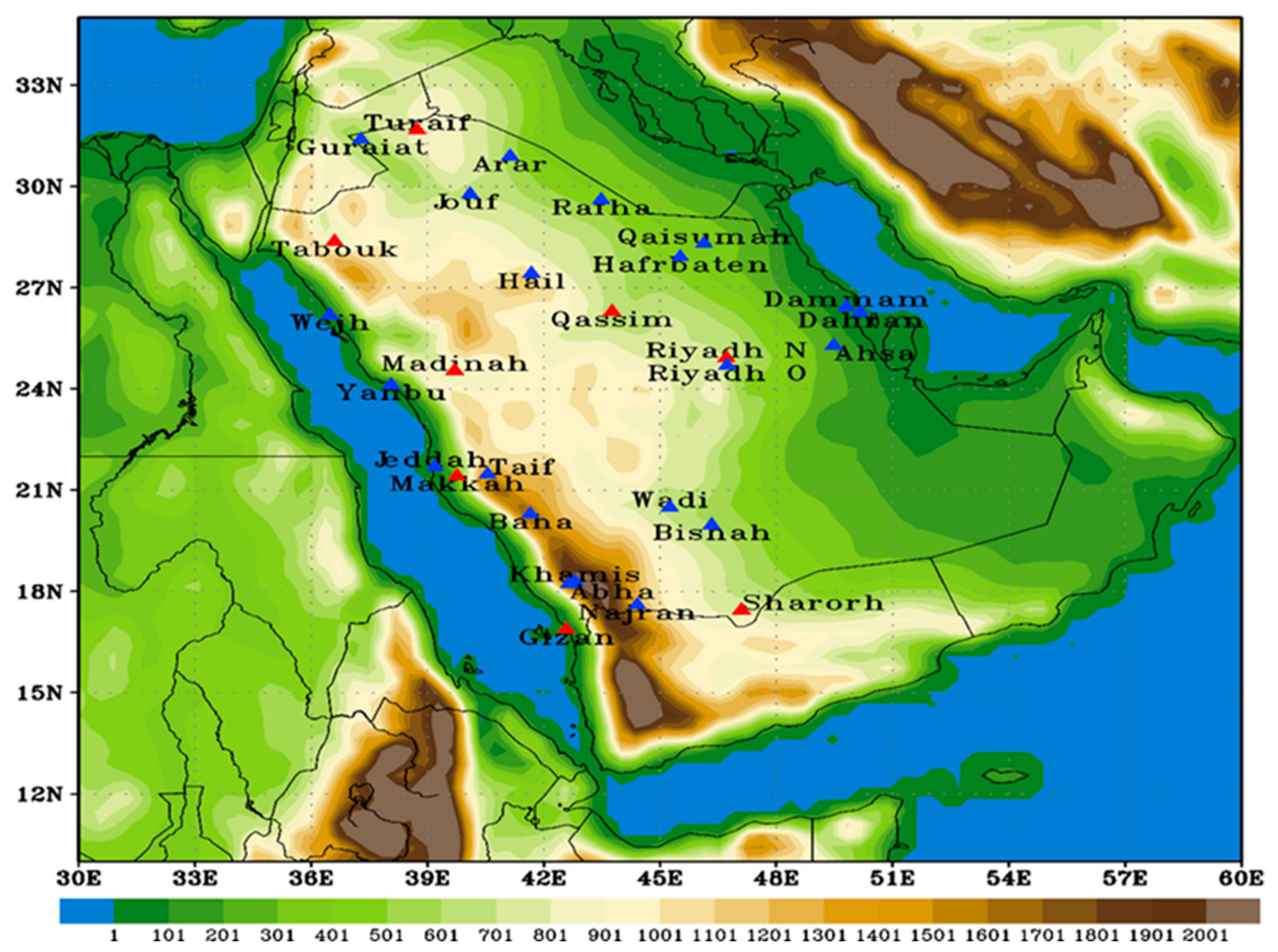
The monthly long-term mean and annual mean are calculated based on monthly TCO and OMR values, while the annual anomalies are calculated for OMR. TCO data at 28 sites (meteorological stations) distributed within the different climatic zones in KSA are extracted from the ERA5 gridded dataset for further statistical procedures and analysis, while, the OMR data are also extracted for three stations in the north (Turaif), middle (Makkah), and south (Sharura) of KSA. Figure 1 and Appendix A (Table A1) clarify the location, name, and altitude of the selected KSA stations.
2.2. Statistical Procedures
Several statistical procedures were employed to study and investigate the long-term climate changes, variability, trends, and the different characteristics of TCO over KSA. To study these climatic characteristics of TCO in a statistically accurate manner, the homogeneity of variances for the climatic TCO data is examined by applying Bartlett’s test [36] considering the normal (Gaussian) distribution of values. This procedure was achieved merely by dividing the TCO data over the considered climatic period into a number of samples (k) with equal subperiods (k ≥ 2). The variance of each k sample () is computed by applying the following formula [37]:
where Σ is the summation of TCO over the series number (n) for each sample K in the different subperiods, is the observed value, and is the temporal mean of observations. Due to dividing the considered study period into an equal sample size, we can define the F-ratio as the ratio between the maximum and minimum variances of samples as follows:
where and .
The obtained F-ratio value is compared to the values given in Table 31 of Pearson and Hartley [38] at the 0.95 confidence level with n − 1 degree of freedom. Based on the F-ratio value, one can examine whether the TCO values in the k samples have equal variances (homogeneous) or not (heterogeneous).
The coefficient of variation (COV) procedure is applied to show and describe the extent of TCO variability over KSA and is calculated as the ratio between the standard deviation (SD) and the temporal mean () as follows:
Gaussian and Binomial [39] low-pass filter techniques are employed to explain the underlying trends, variations, and fluctuations of TCO over the study area and period. These two procedures of low-pass filters are applied to reduce the high-frequency noise and obtain a smoothed TCO time series. Additionally, the Mann–Kendall (M-K) rank correlation non-parametric test [40,41] is employed to identify any possible trends and assess the trend significance in the TCO data series over KSA. The Mann–Kendall rank correlation test sequential steps applied in this study are described in detail by Kendall [42].
The cumulative annual means (CAM) procedure [43] is applied to delineate the annual and decadal fluctuations or “persistence” in the behavior of TCO as defined in Equation (4). The benefit of this method is that it reveals time-varying structures in time series. CAM starts with the first value for TCO () and calculates the second time step of CAM by taking the average of the first two values ( and ) and continues in this manner until it reaches the last CAM time step in which it takes the average of all TCO values () over the total number of years (N). Hence, the last CAM value is equal to the average of all TCO values.
Finally, to identify the abrupt change points and the significant variations of the TCO mean during the selected climate period, the non-parametric Mann–Whitney test for the step trend (rank-based) is employed [44,45,46,47]. According to this test, the time series of the TCO data vector can be divided into two series:
and where each series follows a different distribution function F(x). The non-parametric Mann–Whitney test statistics are given by
where represents the rank of the t observations in the complete series of m observation values. The H0 (null hypothesis) is taken when where α is the significance level of the test.
3. Results and Discussions
3.1. TCO Time Series Homogeneity Test
The homogeneity of total column ozone (TCO) across the selected period and stations in KSA is investigated by the Bartlett test. If the maximum and minimum variances are nearly the same, then the F-ratio will be close to 1; otherwise, the greater the difference between the two variances, the greater the F-ratio value. If the value of the F-ratio is very close to 1, it can be inferred that the data probably show equality of variance (homogeneous), but if the F-ratio is slightly greater than 1, then the tabulated F (Table 31 by Pearson and Hartley [38]) should be used to identify whether the data are homogeneous or heterogeneous [48], where if the F-ratio > tabulated F(k, n − 1), the data will be heterogeneous. The TCO data time series during the period of study (1979–2020) is divided into two samples or subperiods (k = 2) with n = 21 in each subperiod. Therefore, the tabulated critical value for the test at the level of significance of α = 0.05 (0.95 confidence level) and n–1 (20) degrees of freedom is 2.64. By comparing this tabulated critical value (2.64) with the calculated F-ratio for the chosen cities in KSA, it is found that the mean seasonal and annual TCO values at the distributed 28 cities across KSA are homogeneous, as shown in Appendix A (Table A1). These results of the homogeneity test for TCO revealed that the from the ERA5 dataset can be used for further statistical analysis over the different regions in KSA.
3.2. Spatial Distribution of Monthly, Seasonal, and Annual TCO
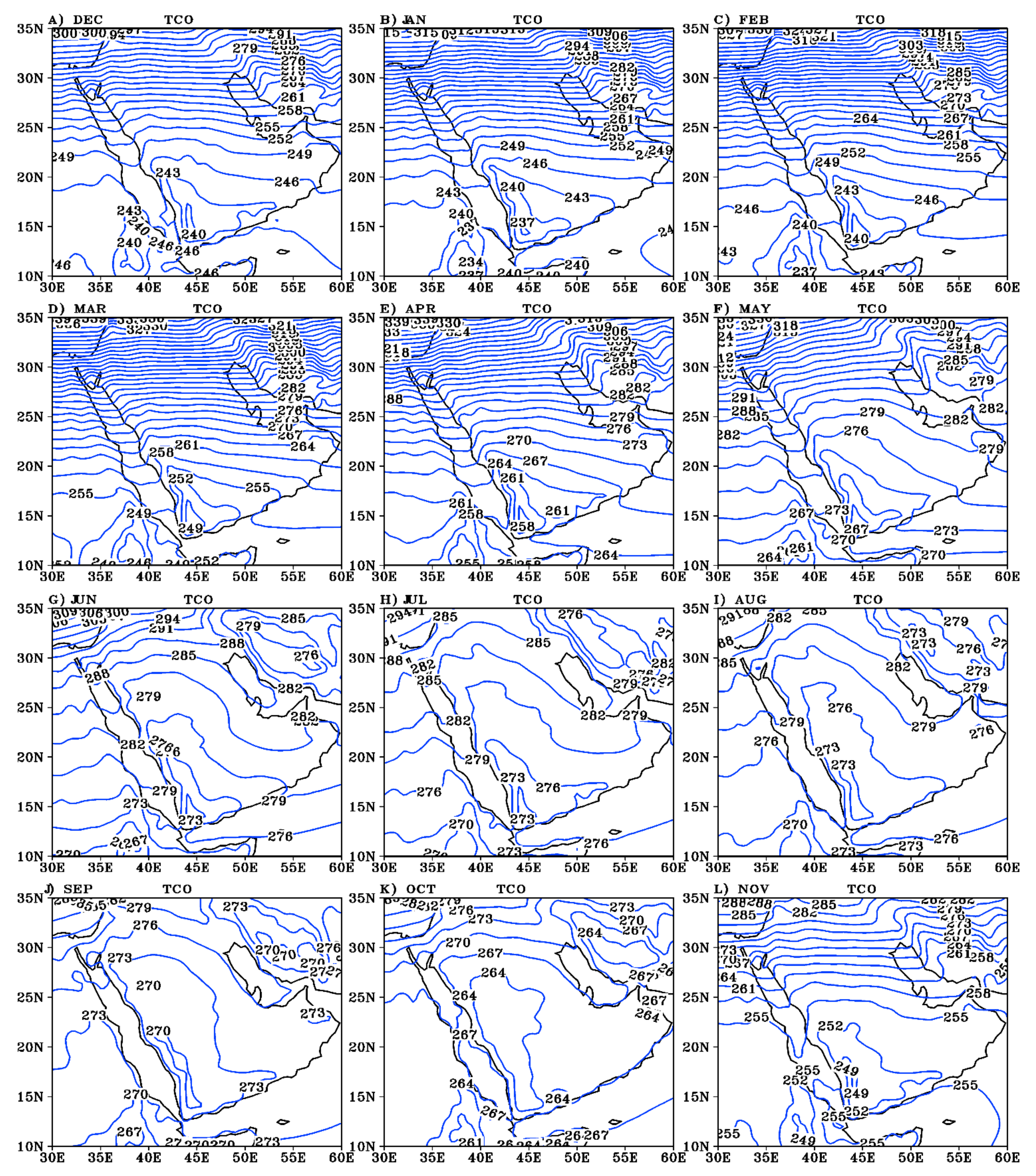
The horizontal distribution of the climatological monthly average of TCO during the 1979–2020 period for each month of the year is shown in Figure 2. It is clear that the monthly average of TCO is a function of latitude as it decreases gradually from northern to southern latitudes especially during the months of winter (December–February) and spring (March–May).
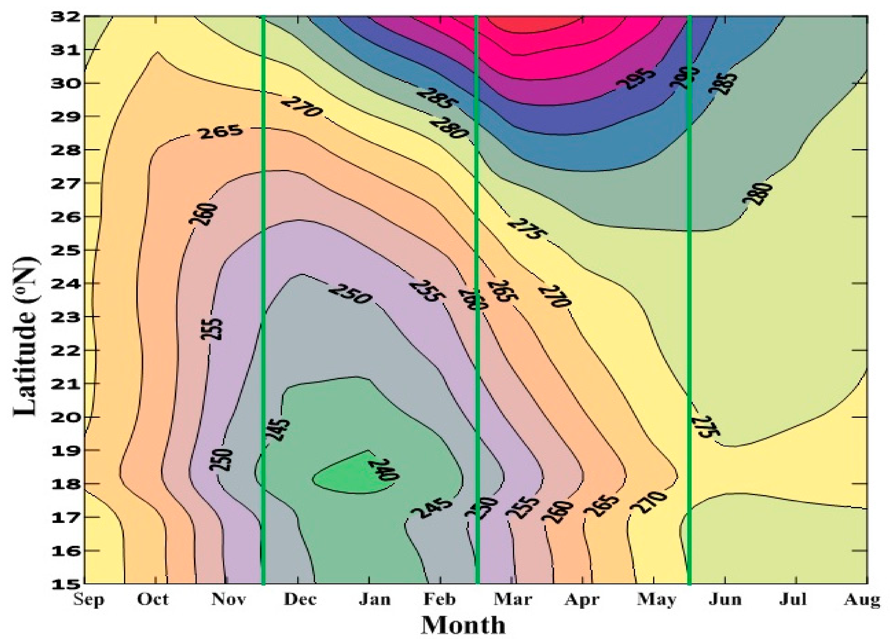
The higher values of TCO over KSA appear north of 20° N through winter and spring months, coinciding with a decrease in the tropopause. Moreover, it is obvious that the latitudinal gradients of TCO are very strong in winter and spring months, especially north of the latitude 20° N, and are nearly equal to three or four times larger than in the summer (June–August) and autumn (September–November) months. Despite the fact that the latitudinal gradient in TCO south of 20° N in winter and spring months is greater than that in summer and autumn months, the values of TCO are smallest in winter and spring months. The lowest values of TCO in the winter and spring months occur in the south, especially in the southwest of KSA. The difference between TCO values in the north and south of KSA reaches more than 50 DU in the winter and spring months. Across the months of the year, the climatological distribution of TCO reflects the significant influence of meteorological parameters and pressure systems on the weather and climate of KSA. The strong latitudinal gradient of TCO with the increase in its quantity at the northern latitudes of KSA in winter and spring months is a result of midlatitude cyclones traveling from west to east that affect the weather of KSA during these two seasons. Dobson and co-workers have established the relation (link) between the meteorological elements on the synoptic scale and TCO from the 1920s onward [49,50,51,52]. Their results revealed that TCO increases with the cold front passage and decreases with the warm front passage, and the maximum values of TCO are noticed near the center of mature surface cyclones and behind developing ones. Furthermore, the surface anticyclones are accompanied by the minimum values of TCO. These relationships between cyclonic/anticyclonic systems and the increasing/decreasing TCO occur as the synoptic weather systems perturb the flow below and above the tropopause and the vertical motion fields into the lower stratosphere, which is associated with trough and ridge patterns [53] and produces most of the short-term variance in TCO. Figure 3 shows the monthly latitudinal variation of TCO at the longitude of 45° E. It illustrates that the highest values of TCO occur during spring in northern latitudes and during summer in southern latitudes. In addition, the minimum TCO values were detected during winter in the southern latitudes and during autumn in the northern latitudes. Thus, a monthly backshift occurs in the highest TCO values as latitudes increase northward.
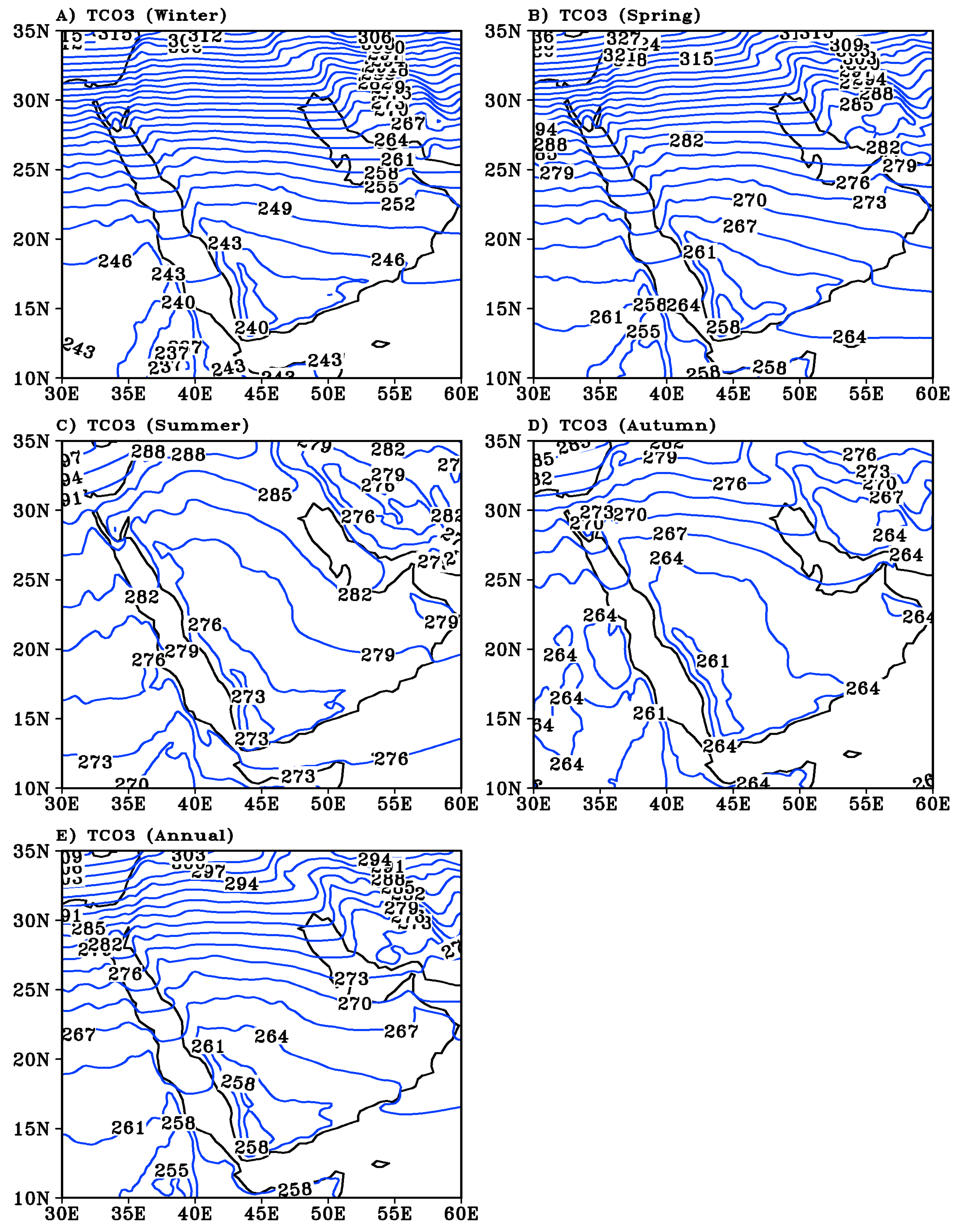
Figure 4A–E displays the average seasonal and annual TCO over KSA. It is obvious that the maximum values of TCO occur in the spring season (Figure 4B) while the lowest values of TCO exist in autumn (Figure 4D) and the second highest values occur in winter (Figure 4A). The winter, spring, and annual values of TCO are a function of its latitude where the maximum values appear in the north while the lower values appear in the south of KSA. The range between the northern and southern values of TCO in spring, winter, annually, autumn, and summer amounts to nearly 56, 53, 33, 15, and 9 DU, respectively. This difference in TCO values between north and south of KSA is what leads to the higher TCO gradient in winter, spring, and annual charts (Figure 4A,B,E). In addition, it is obvious that the values of TCO in the summer season over the middle and south of KSA (south of 25° N) are greater than those corresponding in winter and spring. Figure 4 also illustrates that the variability of TCO at low latitudes is acceptably small at a few DU, whereas it becomes large when extending outside the tropics. The seasonal variations in TCO concentrations can be attributed to both photochemical and dynamic processes [54], where both ozone formation and depletion rely on the incident solar radiation, therefore the photochemical process is affected by the intensity of solar radiation. Ozone is primarily produced in the tropics and transported to higher (middle and polar) latitudes through atmospheric circulation, which plays an important role in local ozone formation at higher latitudes. As solar radiation is nearly the same during April–October, atmospheric circulation (transport) has an important role in seasonal ozone distributions and variations.
3.3. Coefficient of Variation for TCO
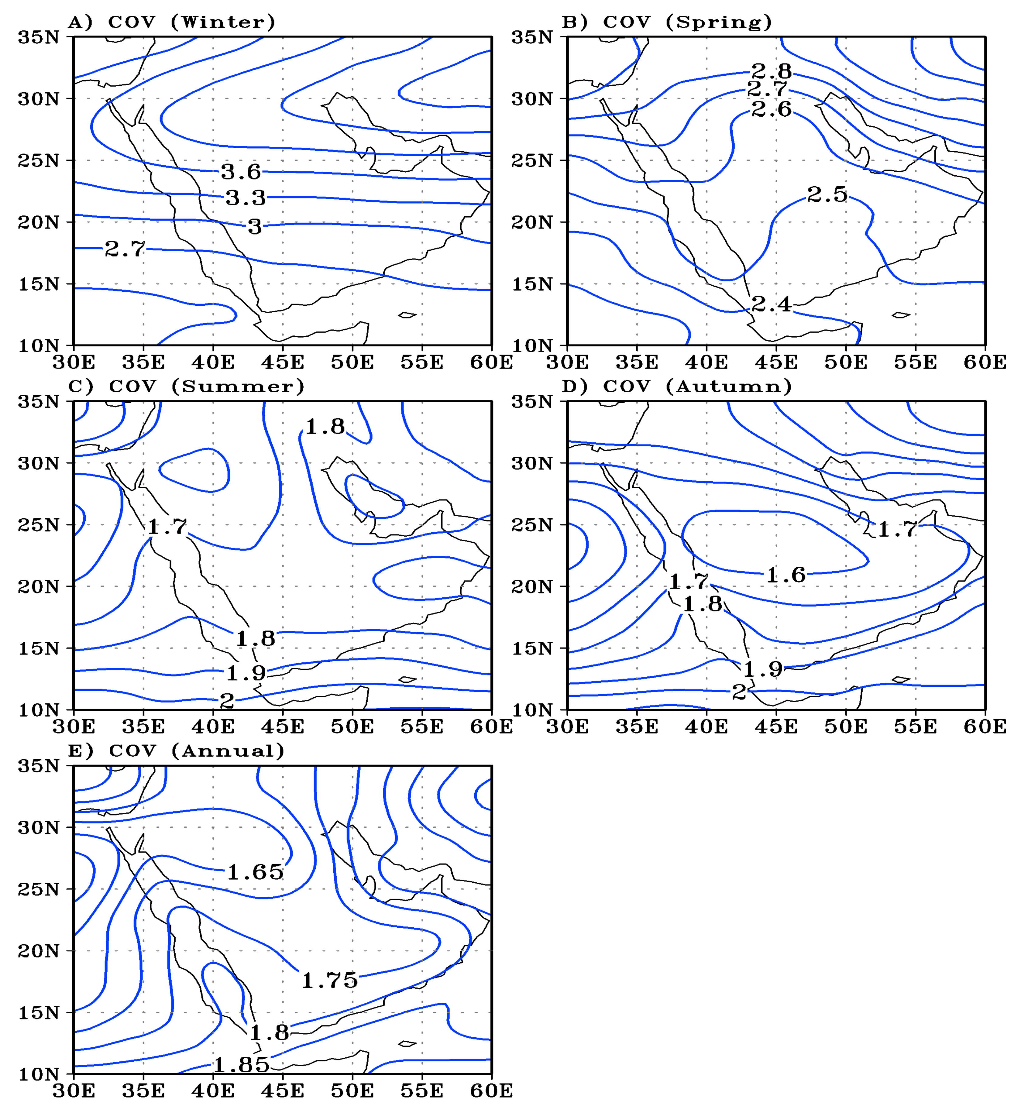
The seasonal (winter, spring, summer, autumn) and annual coefficient of variation (COV) values for TCO are shown in Figure 5. The highest COV values for TCO over KSA occur in winter and spring and the lowest values are detected in summer and autumn. The noticeably high variability of TCO during winter and spring over northern latitudes of KSA is due to the traveling Mediterranean (main and secondary) cyclones. During winter and spring, south of 30° N, the COV gradually decreases southward, and it can be stated that the COV over KSA is a function of latitude during these two seasons south of 30° N. The lowest values of COV in summer and autumn occur over the middle of KSA, reaching less than 1.7 and 1.6 in summer and autumn, respectively. The pattern of the horizontal distribution of COV in the autumn season over KSA is different from that in winter and spring, where its lower values appear in the middle of KSA then increase toward the north and south of KSA. These lowest COV values for TCO over the middle of the Red Sea and KSA in autumn may be a result of the persistence of the northward extension (oscillation) of the Red Sea Trough (RST) from the Sudan monsoon low. Meanwhile, the lowest COV values for TCO in summer appear in the middle of KSA, which may be attributed to the dominant Indian monsoon low over this area.
3.4. Analysis of TCO Trend
The annual values of TCO are calculated during the period 1979–2020 to examine and analyze the different trends at all selected stations in KSA. The means of both simple and sophisticated statistical tools have been applied to study these trends. These methods are (1) the Mann–Kendall rank statistical test and (2) moving filters by applying both Gaussian and binomial low-pass filters. The discussion of the long-term trends and variations of annual TCO are provided in the following sections.
3.4.1. Mann–Kendall (M–K) Test
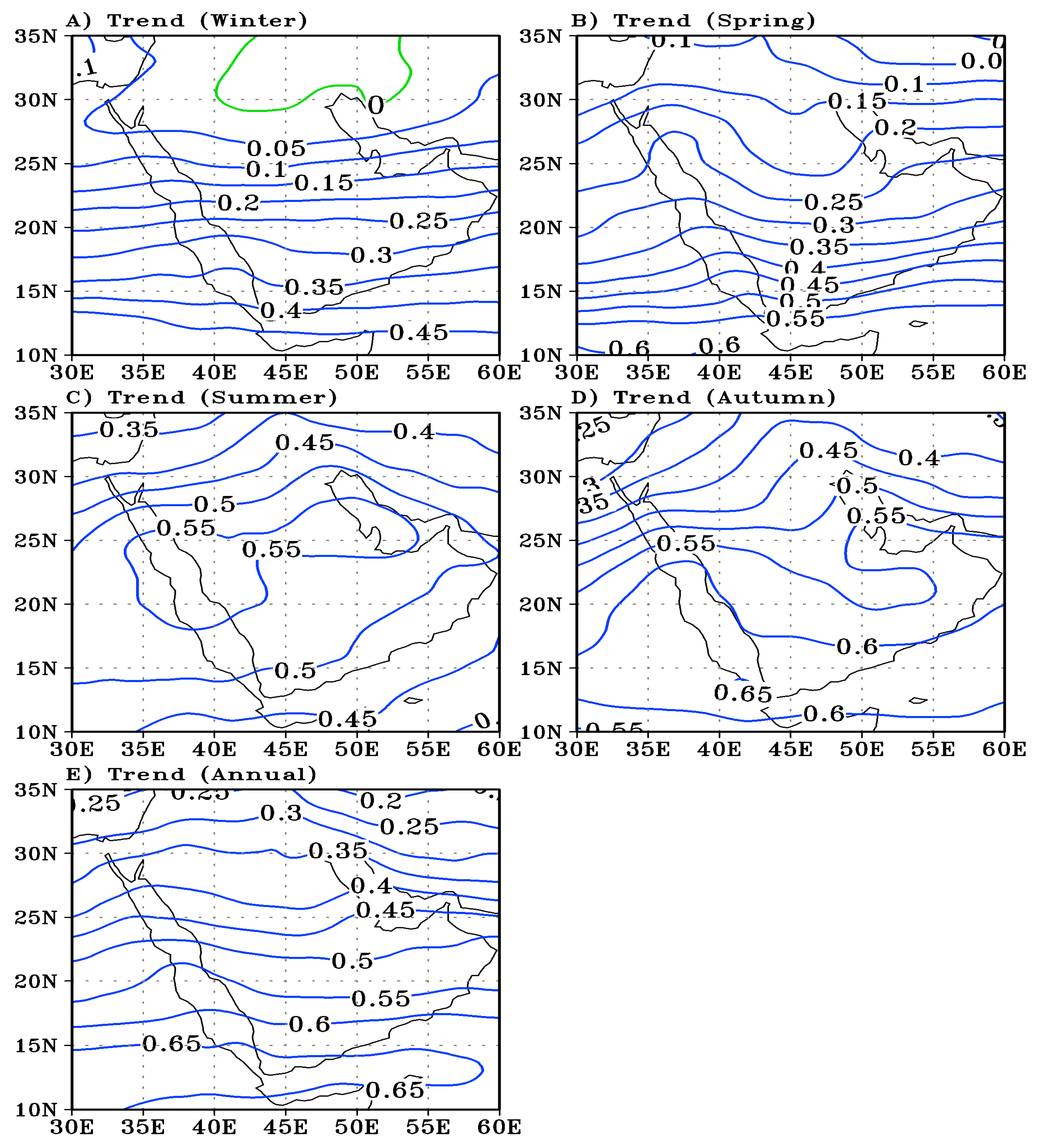
Figure 6 shows the M–K rank correlation test for the seasonal and annual TCO over the KSA region. Generally, positive trends are detected over KSA for both seasonal and annual values of TCO, while the only negative trends in TCO occur in winter north of KSA (north of 30° N between 40–53° E). Moreover, it is noted that the positive values of the trend in the winter season are lower than in other seasons, while the highest positive trend occurs in summer and autumn seasons. The positive values of the trend annually and in winter, spring, and autumn increase gradually southward over KSA. The higher values of the trend in summer appear in the middle of KSA, and decrease in the north and south of KSA.
3.4.2. Fluctuation of TCO Using Moving Filters
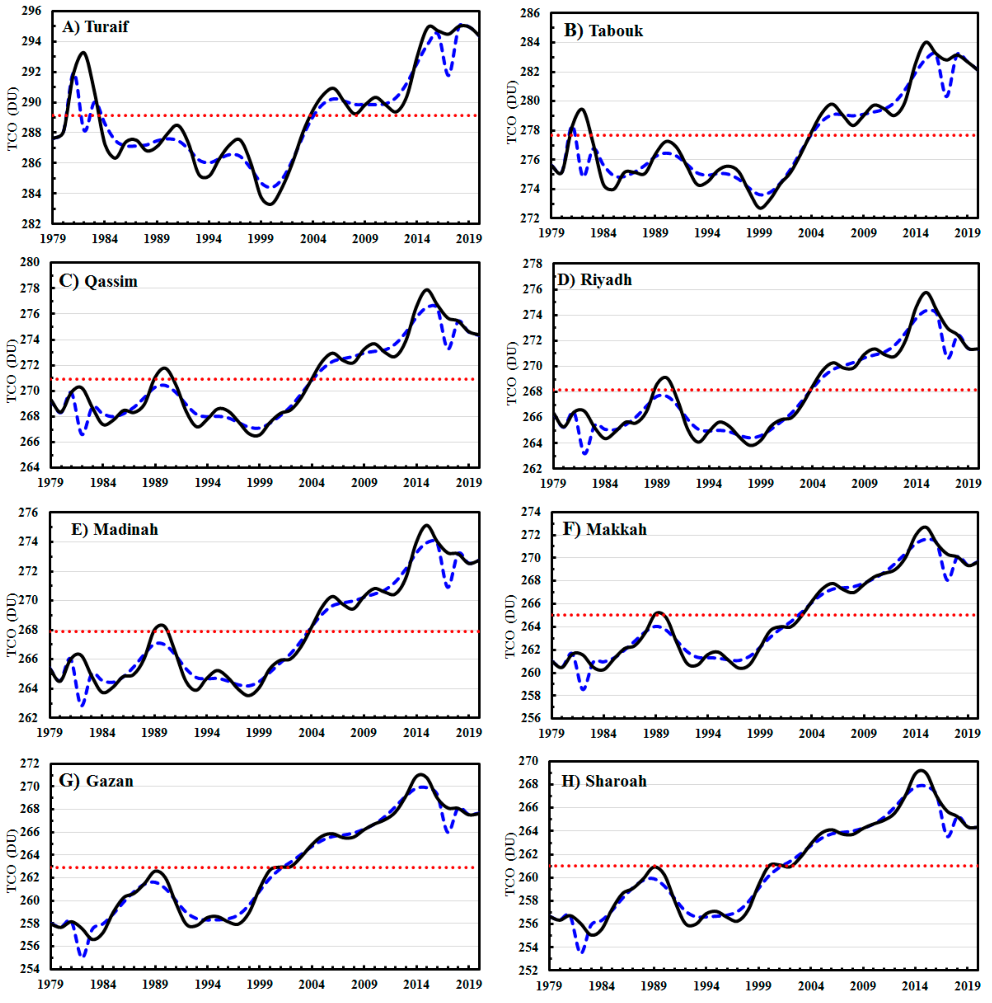
The annual trends and Fluctuations of TCO at the studied stations in KSA are investigated using the Gaussian and binomial low-pass filters. Figure 7 illustrates the results of these two low-pass filters for eight stations. These eight stations were chosen so that they represent the various regions of the KSA, where Tarif and Tabuk represent the north of KSA, while Al-Qassim and Riyadh represent the east and center of KSA. Medina and Makkah represent the west of KSA, while Gizan and Sharurah represent the south of KSA.
Insight into the obtained results from the Gaussian low-pass filter (Figure 7, blue dashed curves) shows that an obvious increase in TCO occurs in the year 1982 at the northern stations, where the annual TCO increased by about 5 DU at Turaif station during the year. A gradual below-normal decrease in TCO appears from 1983 to 2004 with the lowest one in 2000 followed by increasing values above normal up to 2020.
Moreover, the binomial low-pass filter results (Figure 7, solid black curves) demonstrate that there are different regular fluctuations (waves) with different amplitudes and different periods for the east, center, and west KSA stations (Al-Qassim, Riyadh, Medina, and Makkah) during the period 1997 to 2004. An obvious decrease can be noticed during this period except in 1990, and the lowest decrease occurs in 1999. It is obvious that the TCO values are greater than the normal values for these stations from 2004 to 2020, with maximum values in 2015. The results of the southern stations (Gizan and Sharurah) show that a significant decrease occurred in TCO through the years 1979 to 2002 with minimum values in 1983 with an annual decrease of about 6 DU. Generally, it is clear that the values of TCO are less than the average for each station in the middle and south KSA during the period 1979 to 2004, except in 1990, while the values of TCO are greater than the average of each station in KSA during the period 2004 to 2020, with a higher value in 2015.
3.5. Cumulative Annual Means
The cumulative means (CAM), like low-pass filters, have a smoothing effect [55]. The existence of alternating phases of increasing and decreasing TCO that vary in length can be recognized in the annual TCO time series. In this section, the long-term variability of the annual TCO behavior is examined and analyzed with regard to annual TCO time variations. Figure 8 shows the behavior of TCO during the study period (1979–2020) at the chosen eight stations. One can notice that the positive values of the trend in TCO are prevailing at Turaif and Guriat stations from 1981 to1993 (not shown). Furthermore, the positive values of the trend in annual TCO are prevailing at the rest of the stations in KSA along the study period except in 1988, while the negative values of the trend in annual TCO are prevailing at all stations during the period 1993–2006.
3.6. Analysis of TCO Abrupt Change
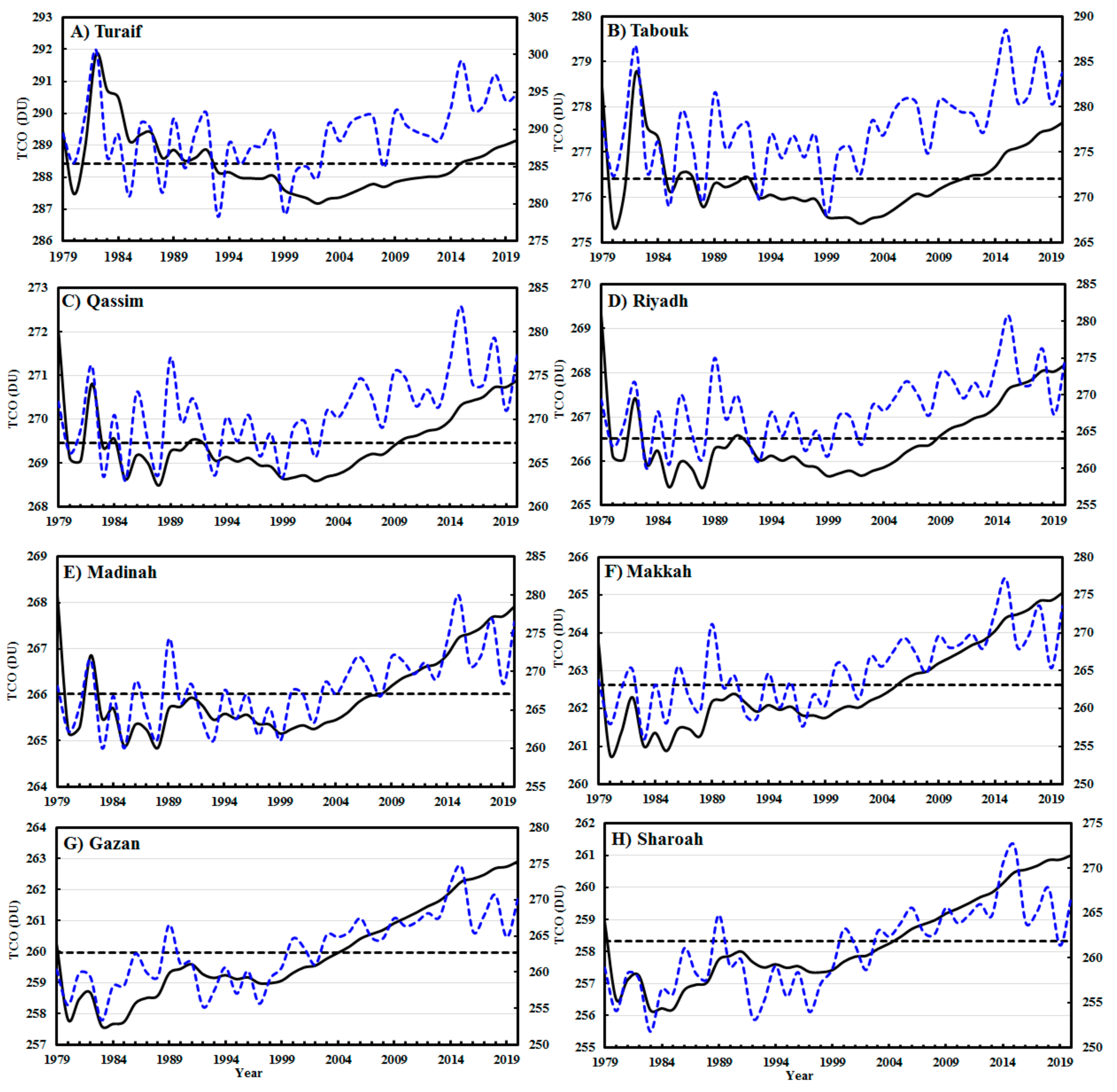
Figure 9 illustrates the Mann–Whitney test results at a 95% confidence level for abrupt changes in the standardized TCO time series for the eight chosen stations over KSA. The TCO departure curves at Turaif station (Figure 9A) indicate that the abrupt change in standardized TCO occurred around 2014 and there is one decreasing and one increasing period in the TCO time series. The decreasing period from 1979 to 2013 has negative departures, where the years of the highest abnormal decreases are 1985, 1988, 1993, and 1999, respectively. Meanwhile, the increasing period from 2015 to 2020 has standardized TCO greater than the climate average by 1.18, where the highest standardized TCO departure (2.11) occurs in 2015. Two abrupt change points have been detected in the TCO time series at Tabouk (Figure 9B). The first point is detected around 2005, while the second point is around 2014. The period of less TCO is from 1979 to 2004, in which the mean standardized TCO is 0.43 less than the average of the whole period. The first period of increasing TCO isfrom 2006 to 2013, in which the mean standardized TCO is 0.35 more than its climate average. The second period of increasing TCO is from 2015 to 2020, in which the mean standardized TCO is 1.3 more than its climate average. Only one abrupt change point has been detected around 2005 in the standardized TCO time series at Qassim and Riyadh, as shown in Figure 9C,D, respectively. The period of lower TCO is from 1979 to 2004, in which the mean standardized TCO is 0.49 and 0.52 less than their climate average, respectively. Furthermore, it is detected that there are two change points (around 2003 and 2014) in the time series of TCO at Madinah and Makkah as illustrated in Figure 9E,F, respectively. It is obvious that the three departure curves fluctuate considerably with one decreasing and two increasing abrupt change points since 1979. The period of lower TCO is from 1979 to 2002, in which the mean standardized TCO is 0.61 and 0.64 less than the climate average for Madinah and Makkah, respectively. The first period of higher TCO is from 2004 to 2013, in which the mean standardized TCO is 0.40 and 0.55 more than their climate average. The second period of higher TCO is between 2015 and 2020, where the mean standardized TCO is 1.33 and 1.32 more than the climate average of Madinah and Makkah, respectively. Additionally, there are three abrupt change points in the TCO at both Gazan (Figure 8G) and Sharoah (Figure 8H) stations. The first point is around 2000, while the second point is around 2012 (Gazan) and 2014 (Sharoah). It is also evident that the departure curves fluctuate considerably with one decreasing and two increasing abrupt changes since 1979. The period of lower TCO is from 1979 to 2000, in which the mean standardized TCO is 0.80 and 0.78 less than the climate average of Gazan and Sharoah, respectively. The first period of higher TCO is from 2001 to 2011 (2001–2013) for Gazan (Sharoah), where the mean standardized TCO is 0.48 (0.56) more than its climate average. The second period of higher TCO is 2013–2020 (2015–2020), where the mean standardized TCO is 1.22 (1.22) more than its climate average at Gazan (Sharoah).
Table 1 explains the years of abrupt change (decreasing or increasing) of the annual TCO over the selected 28 KSA stations using the Mann–Whitney test. It is found that the significantly increasing abrupt change signals occur in 28 stations, where 5 stations (Turaif, guraiat, Arar, Aljouf, and Rafha) have one increasing abrupt change, while the rest of the stations have two increasing abrupt changes. Furthermore, it is clear that the year 2014 has the maximum increasing abrupt change signals for TCO where the signals have been observed at 22 stations. The second maximum increasing abrupt change signal for TCO appears in the year 2005 at 10 stations. The increasing abrupt change signals for TCO in 2000 and 2003 have been observed in eight and six stations, respectively.
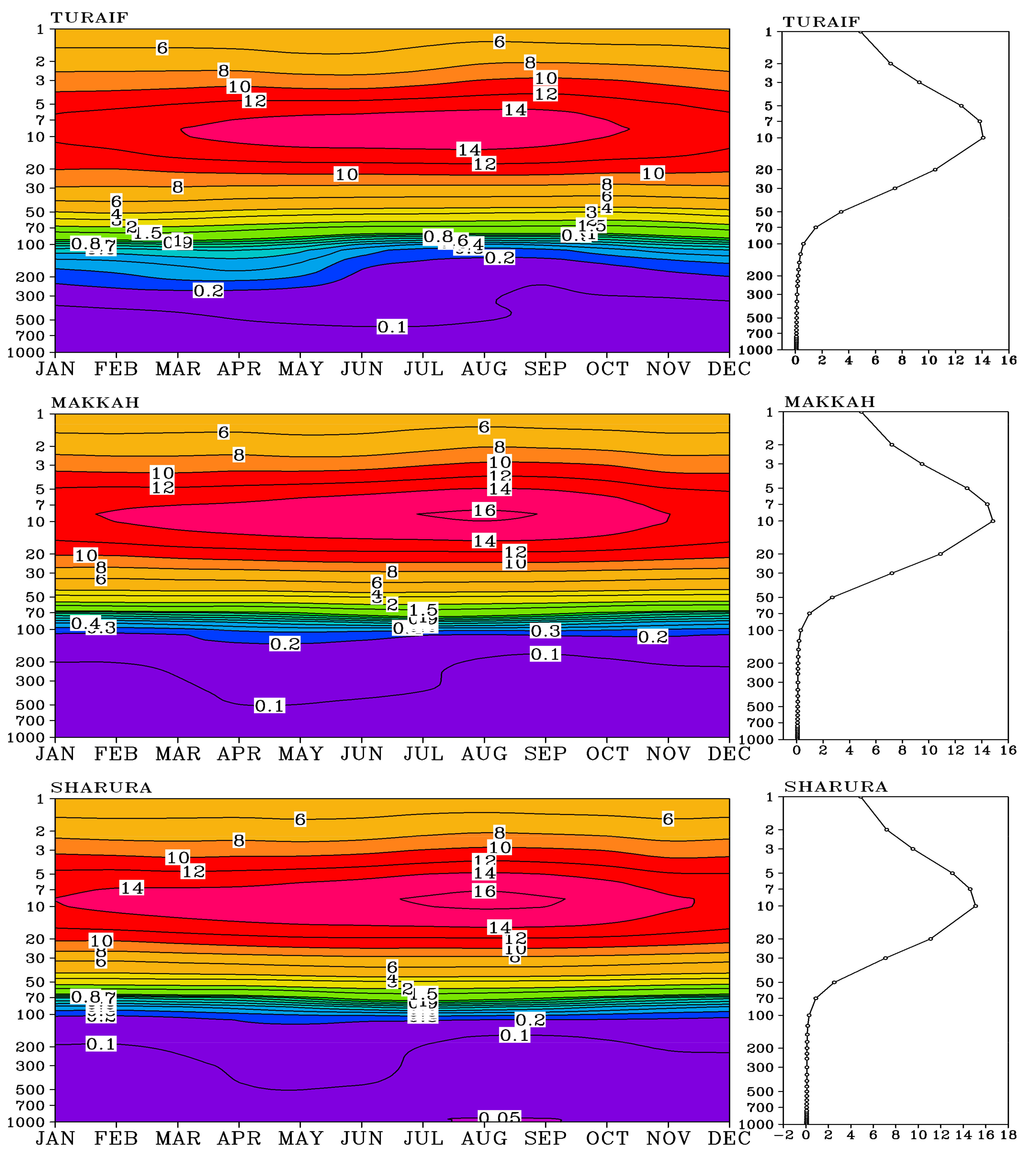
3.7. Time-Height Variations of Ozone Mass Mixing Ratio (OMR)
Figure 10 illustrates the vertical profile (1000–1 hPa) of the climatological monthly mean (left-side) and the long-term mean (right-side) of the ozone mass mixing ratio (OMR) during the period from 1997 to 2020 at Turaif (north of KSA), Makkah (middle of KSA), and Sharura (south of KSA) stations. It is evident that the highest values of OMR (>10 ppm) are found in the layer between 20 and 4 hPa during all months at the selected three stations. The maximum value of OMR exceeds 16 ppm during the summer season and early autumn (June, July, August, and September) and extends to a wide vertical and temporal distribution range at Sharurah compared to Makkah and is not present at Turaif station. Moreover, OMR values gradually decrease above 4 hPa and below 20 hPa reaching 5 ppm at 1 hPa and 50 hPa. The maximum gradient and considerable vertical variation of OMR occur at levels above 100 hPa, particularly between 100 and 50 hPa, while the smallest values of OMR (<0.5 ppm) are found below the level of 100 hPa. In addition, the long-term vertical profile (Figure 10 right-side) shows that the OMR values on all levels below 100 hPa are very small (<0.5 ppm) and have no considerable vertical variation at the selected three stations. Above 100 hPa, the OMR value gradually increases and reaches the maximum value of 15 ppm at Sharurah and Makkah stations and 14 ppm at Turaif station on 10 hPa, then returns again to gradually decrease and reach 5 ppm on 1 hPa at all stations. About 90% of atmospheric ozone is concentrated in the middle of the stratosphere (a height of about 15–35 km) known as the ozone layer, while about 10% resides in the troposphere [11,12]. The balance between sunlight and chemical reactions plays an important role in keeping ozone around its normal level in the stratosphere [56].
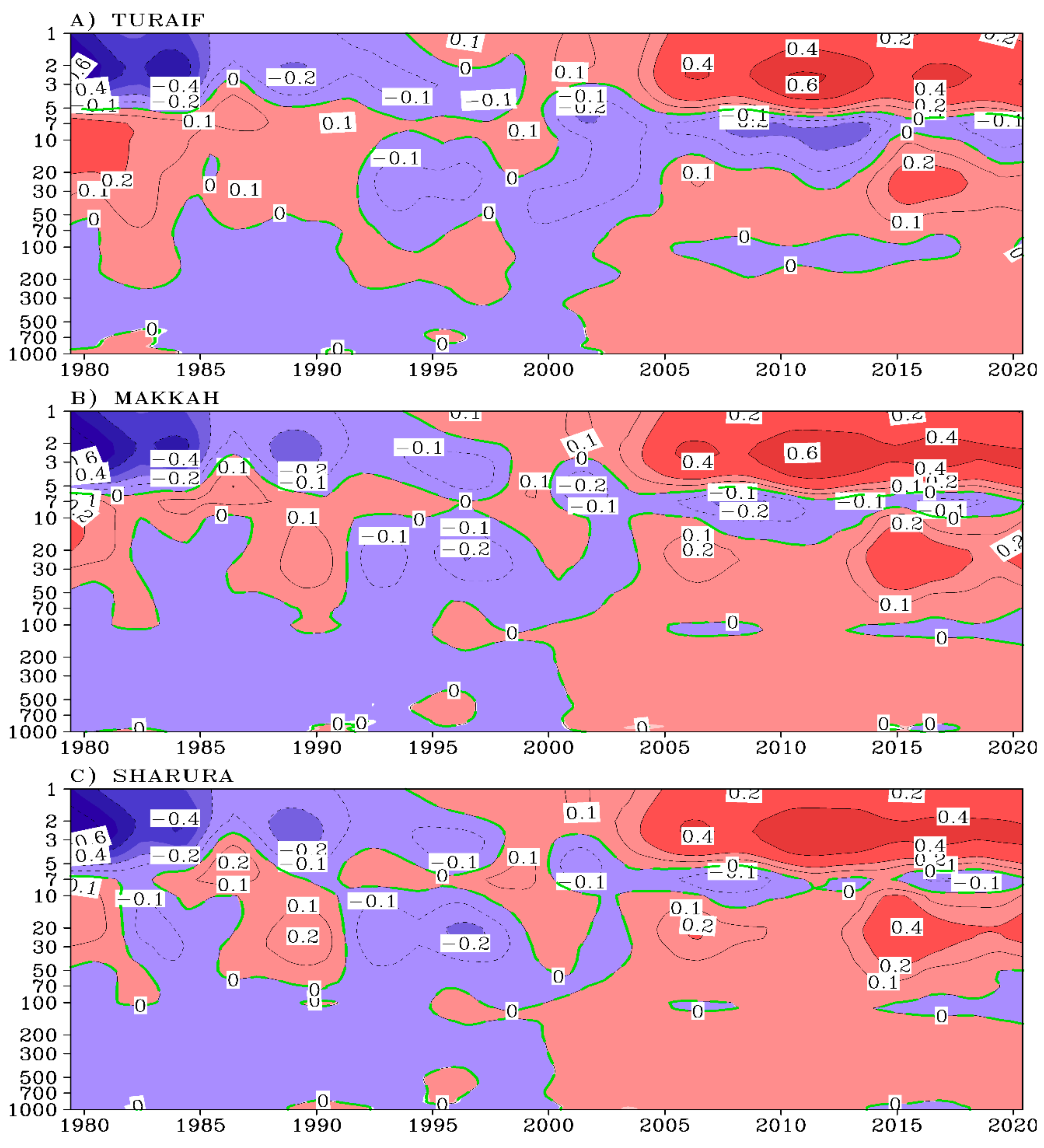
The vertical profile of the annual anomaly of OMR during the period from 1979 to 2020 at the three stations is illustrated in Figure 11. The prevailing values of the annual anomalies of OMR range from 0 to −0.2 ppm (negative anomaly) at all levels below 100 hPa during the period from 1979 to 2001, while there is a positive anomaly during the last two decades (2000–2020) at three stations. The highest vertical variation of the annual anomaly of OMR occurs between the levels of 100 up to 4 hPa with values ranging from −0.6 to +0.6 ppm during the period 1979–2001 and ranging from −0.2 to +0.9 ppm in all years after 2000. The lowest (highest) OMR annual anomaly of <−0.6 ppm (>+0.6 ppm) is detected at levels above 4 hPa during the first six years (2009–2017) at all stations. The negative annual anomaly of OMR predominates before 2001, while the positive annual anomaly prevails after 2001 at most levels except around 10 hPa.
4. Summary and Conclusions
The main aim of this research is to study the long-term variability and trends of TCO over KSA throughout the period of 1979–2020 based on the ECMWF-ERA5 dataset. To achieve this purpose, several statistical procedures were applied, in addition to analyzing the Spatio-temporal distribution of monthly, seasonal, and annual TCO over KSA. Analysis of the results showed that TCO is a function of latitude and time, where the TCO values decrease gradually towards the south and change over the months and seasons of the year. The highest TCO values occur in the spring and winter months, especially in northern KSA, and the lowest values appear in the autumn months. The highest values of the coefficient of variation (COV) for TCO are detected in winter and spring and gradually decrease from southward of KSA, while the lowest COV values appear in summer and autumn. The high values of COV during winter and spring over northern KSA are caused by the impact of the Mediterranean (traveling) cyclones and their interaction with the northward extension of the Red Sea Through from Sudan monsoon low. The Mann–Kendall trend test revealed that seasonal and annual TCO has positive trend values throughout KSA except for some negative trends in winter in the far north of KSA. Additionally, the annual and seasonal positive trend values gradually increase northward over KSA. TCO data were extracted from ERA5 at 28 sites distributed across KSA and identified at ground-based stations to study TCO variability, fluctuations, and abrupt climate change. The Gaussian and binomial low-pass filters indicated that the TCO time series had different fluctuations, being mostly below normal at all stations during 1983–2004 followed by above-normal values up to 2020 with the maximum in 2015. Furthermore, the results of the cumulative annual means (CAM) showed that the annual TCO behavior has long-term variability, as the negative values of the trend in TCO are prevailing through the 1979–2004 period in most stations followed by positive trend values until 2020. The analysis of this abrupt change with the Mann–Whitney test showed that the significant abrupt change signals toward increasing occur at all KSA stations. The stations of Turaif, Guraiat, Arar, Aljouf, and Rafha have one increasing abrupt change, while the rest of the stations have two increasing abrupt changes. In addition, it is clear that the year 2014 has the maximum abrupt change signals toward increasing TCO where the signals have been observed at 22 stations. The second highest abrupt change signals toward increasing TCO appear in the year 2005 at 10 stations. The abrupt change signals towards increasing TCO in 2000 and 2003 have been observed in eight and six stations, respectively. Three stations, Turaif (north of KSA), Makkah (middle of KSA), and Sharura (south of KSA), were identified to interpret the vertical profile (1000–1 hPa) of the climatological monthly mean of the ozone mass mixing ratio (OMR) during the period from 1979 to 2020. It is evident that the highest values of OMR (>10 ppm) are found in the layer between 20 and 4 hPa across all months and the maximum OMR (>16 ppm) occurred during summer and early autumn (June–September). Moreover, OMR gradually decreases above 4 hPa and below 20 hPa, where the maximum gradient and considerable vertical variation are detected at levels above 100 hPa. In addition, the long-term vertical profile shows that the smallest values of OMR (<0.5 ppm) are found at all levels below 100 hPa and have no vertical variation. Above 100 hPa, the OMR value gradually increases and reaches the maximum value (>14 ppm) at three stations at 10 hPa, then returns again to gradually decrease and reach 5 ppm at 1 hPa. Moreover, the negative annual anomalies of OMR (0 to −0.2 ppm) were detected at all levels below 100 hPa during the 1979–2001 period, while a positive anomaly was found during the last two decades (2000–2020) at three stations. The highest vertical variation (−0.6 to +0.6 ppm) of the annual OMR anomaly occurred at levels between 100 and 4 hPa during the 1979–2001 period, while the lowest vertical variation (−0.2 to +0.9 ppm) occurred in all years after 2000. The negative (positive) annual anomaly of OMR prevails before (after) 2001 at most levels except around 10 hPa.
Author Contributions
Conceptualization, S.A.-K., M.A.-M., H.A.B., and A.A.; data curation, M.A.-M., A.A., and A.B.; formal analysis, M.A.-M. and H.A.B.; funding acquisition, S.A.-K.; methodology, S.A.-K., M.A.-M., H.A.B., M.M., and A.B.; project administration, S.A.-K.; resources, M.A.-M.; software, A.A. and A.B.; supervision, S.A.-K., M.A.-M., and H.A.B.; validation, A.A. and M.M.; visualization, A.A. and A.B.; writing—original draft, M.M.; writing—review and editing, H.A.B. All authors have read and agreed to the published version of the manuscript.
Funding
This research was funded by the Deanship of Scientific Research at Princess Nourah Bint Abdulrahman University, through the Research Funding program (Grant No. FRP-1442-21).
Institutional Review Board Statement
Not applicable.
Informed Consent Statement
Not applicable.
Data Availability Statement
The data supporting the findings of this article are included within the article and obtained from https://cds.climate.copernicus.eu/cdsapp#!/dataset/reanalysis-era5-single-levels-monthly-means?tab=form (accessed on 20 February 2021) for TCO and https://cds.climate.copernicus.eu/cdsapp#!/dataset/reanalysis-era5-pressure-levels-monthly-means?tab=form (accessed on 20 February 2021) for OMR.
Acknowledgments
The researchers express their great thanks and appreciation to the Higher Studies and Scientific Research Agency at the University of Princess Nourah Bint Abdulrahman for their support of research project No. (FRP-1442-21) and thank the Princess Nourah Bint Abdulrahman University for providing all the facilities to work in this research, and to all those who contributed to this study.
Conflicts of Interest
All authors declare that they have no conflict of interest.
Appendix A
Name, position, elevation, and homogeneity test for KSA stations.

Table A1.
The name, position, elevation, and Bartlett test (short-cut) results for each selected KSA station.
Table A1.
The name, position, elevation, and Bartlett test (short-cut) results for each selected KSA station.
| No | Station Name | Lon. (° E) | Lat. (° N) | Elev. (m) | Homogeneity (F-Ratio) | ||||
|---|---|---|---|---|---|---|---|---|---|
| Ann. | Win. | Spr. | Sum. | Aut. | |||||
| 1 | Turaif | 38.73 | 31.68 | 855 | 0.42 | 0.55 | 0.31 | 1.427 | 0.94 |
| 2 | Guraiat | 37.28 | 31.40 | 509 | 0.44 | 0.53 | 0.30 | 1.51 | 1.06 |
| 3 | Arar | 41.13 | 30.90 | 555 | 0.46 | 0.79 | 0.32 | 1.77 | 0.97 |
| 4 | Jouf | 40.10 | 29.78 | 689 | 0.47 | 0.89 | 0.24 | 1.99 | 1.04 |
| 5 | Rafha | 43.48 | 29.61 | 449 | 0.59 | 1.03 | 0.29 | 2.48 | 0.94 |
| 6 | Tabouk | 36.60 | 28.38 | 778 | 0.55 | 0.98 | 0.27 | 1.85 | 1.23 |
| 7 | Qaisumah | 46.13 | 28.31 | 358 | 0.79 | 1.27 | 0.32 | 2.70 | 0.83 |
| 8 | Hfr batin | 45.52 | 27.92 | 647 | 0.76 | 1.34 | 0.28 | 2.71 | 0.76 |
| 9 | Hail | 41.68 | 27.43 | 1015 | 0.71 | 1.44 | 0.24 | 1.99 | 0.77 |
| 10 | Dammam | 49.81 | 26.45 | 22 | 1.16 | 1.56 | 0.33 | 2.59 | 0.76 |
| 11 | Qassim | 43.76 | 26.30 | 648 | 0.81 | 1.61 | 0.24 | 1.92 | 0.64 |
| 12 | Dahran | 50.17 | 26.27 | 17 | 1.10 | 1.58 | 0.33 | 2.57 | 0.78 |
| 13 | Wejh | 36.48 | 26.20 | 20 | 0.91 | 1.53 | 0.28 | 2.03 | 1.01 |
| 14 | Ahsa | 49.48 | 25.30 | 179 | 1.01 | 1.68 | 0.29 | 2.02 | 0.62 |
| 15 | Riyadh | 46.71 | 24.93 | 614 | 0.87 | 1.63 | 0.24 | 1.66 | 0.57 |
| 16 | Madinah | 39.70 | 24.55 | 654 | 1.01 | 1.72 | 0.25 | 1.56 | 0.75 |
| 17 | Yanbu | 38.06 | 24.13 | 8 | 1.08 | 1.65 | 0.26 | 1.73 | 0.88 |
| 18 | Jeddah | 39.19 | 21.7 | 240 | 1.12 | 1.66 | 0.24 | 1.46 | 1.10 |
| 19 | Taif | 40.55 | 21.48 | 1478 | 1.07 | 1.64 | 0.23 | 1.32 | 1.04 |
| 20 | Makkah | 39.76 | 21.43 | 240 | 1.12 | 1.63 | 0.24 | 1.45 | 1.10 |
| 21 | Wadi | 45.25 | 20.50 | 629 | 1.07 | 1.80 | 0.22 | 1.50 | 0.93 |
| 22 | Baha | 41.65 | 20.30 | 1672 | 1.16 | 1.68 | 0.24 | 1.38 | 1.26 |
| 23 | Bishah | 46.33 | 19.98 | 1167 | 1.14 | 1.86 | 0.25 | 1.56 | 0.89 |
| 24 | Khamis-M | 42.80 | 18.30 | 2066 | 1.33 | 1.63 | 0.30 | 1.80 | 1.46 |
| 25 | Abha | 42.65 | 18.23 | 2090 | 1.31 | 1.60 | 0.30 | 1.78 | 1.51 |
| 26 | Najran | 44.41 | 17.61 | 1214 | 1.35 | 1.58 | 0.34 | 2.05 | 1.32 |
| 27 | Sharorh | 47.10 | 17.46 | 720 | 1.28 | 1.61 | 0.36 | 2.46 | 1.05 |
| 28 | Gizan | 42.58 | 16.88 | 6 | 1.30 | 1.48 | 0.31 | 2.23 | 1.69 |
References
- Fowler, D.; Amann, M.; Anderson, R.; Ashmore, M.; Cox, P.; Depledge, M.; Derwent, D.; Grennfelt, P.; Hewitt, N.; Hov, O.; et al. Ground-Level Ozone in the 21st Century: Future Trends, Impacts and Policy Implications; The Royal Society: London, UK, 2008; p. 132. [Google Scholar]
- Sinha, P.R.; Sahu, L.K.; Manchanda, R.K.; Sheel, V.; Deushi, M.; Kajino, M.; Schultz, M.G.; Nagendra, N.; Kumar, P.; Trivedi, D.B.; et al. Transport of tropospheric and stratospheric ozone over India: Balloon-borne observations and modeling analysis. Atmos. Environ. 2016, 131, 228–242. [Google Scholar] [CrossRef]
- Saber, A.; Abdel Basset, H.; Morsy, M.; El-Hussainy, F.M.; Eid, M.M. Characteristics of the simulated pollutants and atmospheric conditions over Egypt. NRIAG J. Astron. Geophys. 2020, 9, 402–419. [Google Scholar] [CrossRef]
- Strode, S.A.; Rodriguez, J.M.; Logan, J.A.; Cooper, O.R.; Witte, J.C.; Lamsal, L.N.; Damon, M.; Van Aartsen, B.; Steenrod, S.D.; Strahan, S.E. Trends and variability in surface ozone over the United States. J. Geophys. Res. Atmos. 2015, 120, 9020–9042. [Google Scholar] [CrossRef]
- Ambarsari, N.; Komala, N. Vertical profile variations of ozone in lower stratosphere in Indonesia and influence to upper troposphere ozone based on satellite. In IOP Conference Series: Earth and Environmental Science, Proceedings of the Humanosphere Science School 2017 & The 7th International Symposium for a Sustainable Humanosphere, Bogor, Indonesia, 1–2 November 2017; IOP Publishing: Bristol, UK, 2018; Volume 166. [Google Scholar]
- Stevenson, D.S.; Young, P.J.; Naik, V.; Lamarque, J.F.; Shindell, D.T.; Voulgarakis, A.; Skeie, R.B.; Dalsoren, S.B.; Myhre, G.; Berntsen, T.K.; et al. Tropospheric ozone changes, radiative forcing and attribution to emissions in the Atmospheric Chemistry and Climate Model Intercomparison Project (ACCMIP). Atmos. Chem. Phys. 2013, 13, 3063–3085. [Google Scholar] [CrossRef] [Green Version]
- Kerr, J.B.; McElroy, C.T. Total ozone measurements made with the Brewer ozone spectrophotometer during STOIC. J. Geophys. Res. 1989, 100, 9225–9230. [Google Scholar] [CrossRef]
- Steiner, A.L.; Tawfik, A.B.; Shalaby, A.; Zakey, A.S.; Abdel-Wahab, M.M.; Salah, Z.; Solmon, F.; Sillman, S.; Zaveri, R.A. Climatological simulations of ozone and atmospheric aerosols in the Greater Cairo region. Clim. Res. 2014, 59, 207–228. [Google Scholar] [CrossRef]
- Fioletov, V.E. Ozone climatology, trends, and substances that control ozone. Atmos.-Ocean 2008, 46, 39–67. [Google Scholar] [CrossRef] [Green Version]
- Nogales, C.G.; Ferrari, P.H.; Kantorovich, E.O.; Lage-Marques, J.L. Ozone therapy in medicine and dentistry. J. Contemp. Dent. Pract. 2008, 9, 75–84. [Google Scholar] [CrossRef]
- Komala, N.; Ambarsari, N. Seasonal Variability of Ozone Vertical Profiles in Indonesia Based on AQUA-AIRS Data. In IOP Conference Series: Earth and Environmental Science, Proceedings of the Humanosphere Science School 2017 & The 7th International Symposium for a Sustainable Humanosphere, Bogor, Indonesia, 1–2 November 2017; IOP Publishing: Bristol, UK, 2018; Volume 166. [Google Scholar]
- Langematz, U. Stratospheric ozone: Down and up through the anthropocene. Chem. Texts 2019, 5, 1–12. [Google Scholar] [CrossRef] [Green Version]
- Rozanov, E. Preface: Ozone Evolution in the Past and Future. Atmosphere 2020, 11, 709. [Google Scholar] [CrossRef]
- WMO (World Meteorological Organization). Scientific Assessment of Ozone Depletion: 2018, Global Ozone Research and Monitoring Project-Report No. 58; WMO: Geneva, Switzerland, 2018; 588p. [Google Scholar]
- Bais, A.F.; Lucas, R.M.; Bornman, J.F.; Williamson, C.E.; Sulzberger, B.; Austin, A.T.; Wilson, S.R.; Andrady, A.L.; Bernhard, G.; Aucamp, P.J.; et al. Environmental effects of ozone depletion, UV radiation, and interactions with climate change: UNEP Environmental E_ects Assessment Panel, update 2019. Photochem. Photobiol. Sci. 2020, 19, 542–584. [Google Scholar]
- Weber, M.; Dikty, S.; Burrows, J.P.; Garny, H.; Dameris, M.; Kubin, A.; Abalichin, J.; Langematz, U. The Brewer-Dobson circulation and total ozone from seasonal to decadal time scales. Atmos. Chem. Phys. 2011, 11, 11221–11235. [Google Scholar] [CrossRef] [Green Version]
- Banerjee, T.; Singh, S.B.; Srivastava, R.K. Development and performance evaluation of statistical models correlating air pollutants and meteorological variables at Pantnagar, India. Atmos. Res. 2011, 99, 505–517. [Google Scholar] [CrossRef]
- Shukla, K.; Srivastava, P.K.; Banerjee, T.; Aneja, V.P. Trend and variability of atmospheric ozone over middle Indo-Gangetic Plain: Impacts of seasonality and precursor gases. Environ. Sci. Pollut. Res. 2017, 24, 164–179. [Google Scholar] [CrossRef]
- Bencherif, H.; Toihir, A.M.; Mbatha, N.; Sivakumar, V.; Du Preez, D.J.; Bègue, N.; Coetzee, G. Ozone Variability and Trend Estimates from 20-Years of Ground-Based and Satellite Observations at Irene Station, South Africa. Atmosphere 2020, 11, 1216. [Google Scholar] [CrossRef]
- Lawrence, M.G. Export of air pollution from southern Asia and its large-scale effects. Air Pollut. 2004, 131–172. [Google Scholar]
- Duncan, B.N.; West, J.J.; Yoshida, Y.; Fiore, A.M.; Ziemke, J.R. The influence of European pollution on ozone in the Near East and northern Africa. Atmos. Chem. Phys. 2008, 8, 2267–2283. [Google Scholar] [CrossRef] [Green Version]
- Liu, J.J.; Jones, D.B.; Worden, J.R.; Noone, D.; Parrington, M.; Kar, J. Analysis of the summertime buildup of tropospheric ozone abundances over the Middle East and North Africa as observed by the Tropospheric Emission Spectrometer instrument. J. Geophys. Res. Atmos. 2009, 114. [Google Scholar] [CrossRef]
- Liu, J.J. Tropospheric Ozone over the Middle East and Its Interannual Variability: An Integrated Analysis with Satellite Observations and a Global Chemical Transport Model. Ph.D. Thesis, University of Toronto, Toronto, ON, Canada, 2010. [Google Scholar]
- Xu, W.; Xu, X.; Lin, M.; Lin, W.; Tarasick, D.; Tang, J.; Ma, J.; Zheng, X. Long-term trends of surface ozone and its influencing factors at the Mt Waliguan GAW station, China–Part 2: The roles of anthropogenic emissions and climate variability. Atmos. Chem. Phys. 2018, 18, 773–798. [Google Scholar] [CrossRef] [Green Version]
- Liu, J.; Tarasick, D.W.; Fioletov, V.E.; McLinden, C.; Zhao, T.; Gong, S.; Sioris, C.; Jin, J.J.; Liu, G.; Moeini, O. A global ozone climatology from ozone soundings via trajectory mapping: A stratospheric perspective. Atmos. Chem. Phys. 2013, 13, 11441–11464. [Google Scholar] [CrossRef] [Green Version]
- World Meteorological Organization (WMO). Scientific Assessment of Ozone Depletion: Global Ozone Research and Monitoring Project; Report No. 52; WMO: Geneva, Switzerland, 2011. [Google Scholar]
- Solomon, S. Stratospheric ozone depletion: A review of concepts and history. Rev. Geophys. 1999, 37, 275–316. [Google Scholar] [CrossRef]
- Chandra, S.; Varotsos, C.; Flynn, L.E. The mid-latitude total ozone trends in the northern hemisphere. Geophys. Res. Lett. 1996, 23, 555–558. [Google Scholar] [CrossRef]
- Ogunniyi, J.; Sivakumar, V. Ozone climatology and its variability from ground based and satellite observations over Irene, South Africa (25.5° S; 28.1° E)—Part 2: Total column ozone variations. Atmósfera 2018, 31, 11–24. [Google Scholar] [CrossRef] [Green Version]
- Badawy, A.; Basset, H.A.; Eid, M. Spatial and Temporal Variations of Total Column Ozone over Egypt. J. Earth Atmos. Sci. 2017, 2, 1–16. [Google Scholar]
- Davis, S.M.; Hegglin, M.I.; Fujiwara, M.; Dragani, R.; Harada, Y.; Kobayashi, C.; Long, C.; Manney, G.L.; Nash, E.R.; Potter, G.L.; et al. Assessment of upper tropospheric and stratospheric water vapor and ozone in reanalyses as part of S-RIP. Atmos. Chem. Phys. 2017, 17, 12743–12778. [Google Scholar] [CrossRef] [Green Version]
- Hersbach, H.; Bell, B.; Berrisford, P.; Hirahara, S.; Horányi, A.; Muñoz-Sabater, J.; Nicolas, J.; Peubey, C.; Radu, R.; Schepers, D.; et al. The ERA5 global reanalysis. Q. J. R. Meteorol. Soc. 2020, 146, 1999–2049. [Google Scholar] [CrossRef]
- Cariolle, D.; Deque, M. Southern hemisphere medium-scale waves and total ozone disturbances in a spectral general circulation model. J. Geophys. Res. 1986, 91, 10825–10846. [Google Scholar] [CrossRef]
- Cariolle, D.; Teyssèdre, H. A revised linear ozone photochemistry parameterization for use in transport and general circulation models: Multi-annual simulations. Atmos. Chem. Phys. 2007, 7, 2183–2196. [Google Scholar] [CrossRef] [Green Version]
- Hersbach, H.; Bell, B.; Berrisford, P.; Biavati, G.; Dee, D.; Horányi, A.; Nicolas, J.; Peubey, C.; Radu, R.; Rozum, I.; et al. The ERA5 Global Atmospheric Reanalysis at ECMWF as a comprehensive dataset for climate data homogenization, climate variability, trends and extremes. Geophys. Res. Abstr. 2019, 21, 10826. [Google Scholar]
- Bartlett, M.S. Properties of sufficiency and statistical tests. Proceedings of the Royal Society of London. Ser. A Math. Phys. Sci. 1937, 160, 268–282. [Google Scholar]
- Mitchell, J.M.; Dzerdzeevskii, B.; Flohn, H.; Hofmery, W.L. Climatic Change; WMO Tech. Note 79. WMO No. 195. TP-100; WMO: Geneva, Switzerland, 1966; 79p. [Google Scholar]
- Pearson, E.S.; Hartley, H.O. Biometrika Tables for Statisticians; Cambridge University Press: Cambridge, UK, 1958; 240p. [Google Scholar]
- Tyson, P.D.; Dyer, T.G.; Mametse, M.N. Secular changes in South African rainfall: 1880 to 1972. Q. J. R. Meteorol. Soc. 1975, 101, 817–833. [Google Scholar] [CrossRef]
- Sneyers, R. On the Statistical Analysis of Series of Observations; Technical Note, No. 143; World Meteorological Organization (WMO): Geneva, Switzerland, 1990; 192p. [Google Scholar]
- Schonwiese, C.D.; Rapp, J. Climate Trend Atlas of Europe Based on Observations 1891–1990; Kluer Academic Publishers: Dordrecht, The Netherlands, 1997. [Google Scholar]
- Kendall, M.G. The Measurement of Rank Correlation. Rank Correlation Methods, 4th ed.; Charles Griffin: London, UK, 1970; pp. 1–18. [Google Scholar]
- Pavia, E.G.; Graef, F. The recent rainfall climatology of the Mediterranean Californias. J. Clim. 2002, 15, 2697–2701. [Google Scholar] [CrossRef]
- Wilcoxon, F. Individual comparisons by ranking methods. Biom. Bull. 1945, 1, 80–83. [Google Scholar] [CrossRef]
- Mann, H.B.; Whitney, D.R. On a test of whether one of two random variables is stochastically larger than the other. Ann. Math. Stat. 1947, 18, 50–60. [Google Scholar] [CrossRef]
- Conover, W.J. Practical Nonparametric Statistics, 1st ed.; John Wiley & Sons: New York, NY, USA, 1971; pp. 97–104. [Google Scholar]
- Mendenhall, W.; Wackerly, D.D.; Sheaffer, R.L. Mathematical Statistics with Applications, 4th ed.; PWS-Kent: Boston, MA, USA, 1990. [Google Scholar]
- Zimmerman, D.W. A note on preliminary tests of equality of variances. Br. J. Math. Stat. Psychol. 2004, 57, 173–181. [Google Scholar] [CrossRef] [PubMed]
- Dobson, G.M.B.; Harrison, D.N. Measurements of the amount of ozone in the Earth’s atmosphere and its relation to other geophysical conditions. Proc. R. Soc. Lond. Ser. A Contain. Pap. A Math. Phys. Character 1926, 110, 660–693. [Google Scholar] [CrossRef]
- Dobson, A.D. Reminiscences of Arthur Dudley Dobson, Engineer, 1841–1930; Whitcombe and Tombs, Limited: Auckland, New Zealand, 1930. [Google Scholar]
- Dobson, G.M.B.; Harrison, D.N.; Lawrence, J. Measurements of the amount of ozone in the Earth’s atmosphere and its relation to other geophysical conditions—Part III. Proc. R. Soc. Lond. Ser. A Contain. Pap. A Math. Phys. Character 1929, 122, 456–486. [Google Scholar]
- Dobson, G.M.B.; Brewer, A.W.; Cwilong, B.M. Bakerian lecture Meteorology of the lower stratosphere. Proc. R. Soc. Lond. Ser. A Math. Phys. Sci. 1946, 185, 144–175. [Google Scholar]
- Reed, R.J. The role of vertical motions in ozone-weather relationships. J. Atmos. Sci. 1950, 7, 263–267. [Google Scholar] [CrossRef]
- Aesawy, A.M.; Mayhoub, A.B.; Sharobim, W.M. Seasonal variation of photochemical and dynamical components of ozone in subtropical regions. Theor. Appl. Climatol. 1994, 49, 241–247. [Google Scholar] [CrossRef]
- Lozowski, E.P.; Charlton, R.B.; Nguyen, C.D.; Wilson, J.D. The use of cumulative monthly mean temperature anomalies in the analysis of local interannual climate variability. J. Clim. 1989, 2, 1059–1068. [Google Scholar] [CrossRef] [Green Version]
- Agarwal, B.; Agarwal, S.; Rao, J. Ozone and Environment. Radiat. Prot. Environ. 2011, 34, 164–165. [Google Scholar] [CrossRef]
Figure 1.
The name and location of KSA stations with shaded elevations (m).

Figure 2.
The horizontal distribution of the monthly average values (A–L) of TCO (1979–2020) for each month of the year.
Figure 2.
The horizontal distribution of the monthly average values (A–L) of TCO (1979–2020) for each month of the year.

Figure 3.
The monthly latitudinal variation of TCO at a longitude of 45°.

Figure 4.
The horizontal distribution of the seasonal (A–D) and annual (E) average values of TCO (1979–2020).
Figure 4.
The horizontal distribution of the seasonal (A–D) and annual (E) average values of TCO (1979–2020).

Figure 5.
The coefficient of variation of annual (E), winter (A), spring (B), summer (C), and autumn (D) TCO for KSA.
Figure 5.
The coefficient of variation of annual (E), winter (A), spring (B), summer (C), and autumn (D) TCO for KSA.

Figure 6.
The trend values of the annual (E), winter (A), spring (B), summer (C), and autumn (D) TCO of KSA stations by Mann–Kendall rank correlation test.
Figure 6.
The trend values of the annual (E), winter (A), spring (B), summer (C), and autumn (D) TCO of KSA stations by Mann–Kendall rank correlation test.

Figure 7.
The fluctuations of the annual mean of TCO at the stations Turaif (A), Tabouk (B), Qassim (C), Riyadh (D), Madinah (E), Makkah (F), Gizan (G) and Sharorh (H). …… mean annual of TCO, ــــــــــ TCO binomial low-pass filter, ------ TCO Gaussian low-pass filter.
Figure 7.
The fluctuations of the annual mean of TCO at the stations Turaif (A), Tabouk (B), Qassim (C), Riyadh (D), Madinah (E), Makkah (F), Gizan (G) and Sharorh (H). …… mean annual of TCO, ــــــــــ TCO binomial low-pass filter, ------ TCO Gaussian low-pass filter.

Figure 8.
The cumulative annual mean (CAM) for TCO time series and the averaged CAM of TCO at the stations Turaif (A), Tabouk (B), Qassim (C), Riyadh (D), Madinah (E), Makkah (F), Gizan (G), and Sharorh (H). --------- The means of TCO CAM, ـــــــــ the TCO CAM time series, and ------ the ERA-5 TCO time series.

Figure 9.
Shifts in the mean for standardization of the annual mean of TCO at the stations Turaif (A), Tabouk (B), Qassim (C), Riyadh (D), Madinah (E), Makkah (F), Gizan (G), and Sharorh (H). Probability = 0.1, cutoff length = 10, Huber parameter = 2.
Figure 9.
Shifts in the mean for standardization of the annual mean of TCO at the stations Turaif (A), Tabouk (B), Qassim (C), Riyadh (D), Madinah (E), Makkah (F), Gizan (G), and Sharorh (H). Probability = 0.1, cutoff length = 10, Huber parameter = 2.

Figure 10.
The mean of monthly height vertical profile of OMR from 1000 to 1 hPa from 1997 to 2020 for the Turaif, Makkah, and Sharura stations.
Figure 10.
The mean of monthly height vertical profile of OMR from 1000 to 1 hPa from 1997 to 2020 for the Turaif, Makkah, and Sharura stations.

Figure 11.
The deviation of annual height vertical profile (1000 to 1 hPa) of OMR from its long-term mean throughout the period 1979-2020 for the Turaif (A), Makkah (B), and Sharura (C) stations.
Figure 11.
The deviation of annual height vertical profile (1000 to 1 hPa) of OMR from its long-term mean throughout the period 1979-2020 for the Turaif (A), Makkah (B), and Sharura (C) stations.

Table 1.
The detected years of abrupt change (decreasing or increasing) of the annual TCO of the KSA stations (28) by the Mann–Kendall rank statistic test.
Table 1.
The detected years of abrupt change (decreasing or increasing) of the annual TCO of the KSA stations (28) by the Mann–Kendall rank statistic test.
| Year | Stations Name | No. of Stations |
|---|---|---|
| 2000 | Wadi Dawaser–Baha–Bishah-Khamis Mushate-Abha- Najran–Sharorh-Gizan | 8 |
| 2003 | Ahsa–Madinah–Yanbu–Jeddah–Taif-Makkah | 6 |
| 2005 | Tabouk-Qaisumah-Hfr Batin–Hail-Dammam–Qassim-Dahran-Wejh-Riyadh-N- Riyadh-O | 10 |
| 2009 | Rafha | 1 |
| 2012 | Guraiat- Abha- Gizan | 3 |
| 2014 | Turaif-Arar-Jouf- Tabouk-Hfr Batin- Hail- Dammam- Dahran–Wejh-Ahsa-Riyadh_N- Riyadh_O- Madinah- Yanbu- Jeddah- Taif- Makkah-Wadi Dawaser- Baha- Bishah- Najran- Sharorh | 22 |
| 2019 | Qaisumah | 1 |
| 2020 | Qassim-Riyadh-N | 2 |
Publisher’s Note: MDPI stays neutral with regard to jurisdictional claims in published maps and institutional affiliations. |
© 2021 by the authors. Licensee MDPI, Basel, Switzerland. This article is an open access article distributed under the terms and conditions of the Creative Commons Attribution (CC BY) license (https://creativecommons.org/licenses/by/4.0/).
Share and Cite
MDPI and ACS Style
Al-Kallas, S.; Al-Mutairi, M.; Abdel Basset, H.; Abdeldym, A.; Morsy, M.; Badawy, A. Climatological Study of Ozone over Saudi Arabia. Atmosphere 2021, 12, 1275. https://doi.org/10.3390/atmos12101275
AMA Style
Al-Kallas S, Al-Mutairi M, Abdel Basset H, Abdeldym A, Morsy M, Badawy A. Climatological Study of Ozone over Saudi Arabia. Atmosphere. 2021; 12(10):1275. https://doi.org/10.3390/atmos12101275
Chicago/Turabian StyleAl-Kallas, Saleha, Motirh Al-Mutairi, Heshmat Abdel Basset, Abdallah Abdeldym, Mostafa Morsy, and Ayman Badawy. 2021. "Climatological Study of Ozone over Saudi Arabia" Atmosphere 12, no. 10: 1275. https://doi.org/10.3390/atmos12101275
Note that from the first issue of 2016, this journal uses article numbers instead of page numbers. See further details here.