
Regional and Local Impacts of the ENSO and IOD Events of 2015 and 2016 on the Indian Summer Monsoon—A Bhutan Case Study


1
Department of Physical Geography, Stockholm University, SE-10691 Stockholm, Sweden
2
Royal Society for Protection of Nature, Thimphu 11001, Bhutan
*
Author to whom correspondence should be addressed.
Atmosphere 2021, 12(8), 954; https://doi.org/10.3390/atmos12080954
Submission received: 7 June 2021
/
Revised: 20 July 2021
/
Accepted: 22 July 2021
/
Published: 24 July 2021
(This article belongs to the Special Issue Tropical Ocean-Atmosphere Interaction and Climate Change)
Abstract
:The Indian Summer Monsoon (ISM) plays a vital role in the livelihoods and economy of those living on the Indian subcontinent, including the small, mountainous country of Bhutan. The ISM fluctuates over varying temporal scales and its variability is related to many internal and external factors including the El Niño Southern Oscillation (ENSO) and the Indian Ocean Dipole (IOD). In 2015, a Super El Niño occurred in the tropical Pacific alongside a positive IOD in the Indian Ocean and was followed in 2016 by a simultaneous La Niña and negative IOD. These events had worldwide repercussions. However, it is unclear how the ISM was affected during this time, both at a regional scale over the whole ISM area and at a local scale over Bhutan. First, an evaluation of data products comparing ERA5 reanalysis, TRMM and GPM satellite, and GPCC precipitation products against weather station measurements from Bhutan, indicated that ERA5 reanalysis was suitable to investigate ISM change in these two years. The reanalysis datasets showed that there was disruption to the ISM during this period, with a late onset of the monsoon in 2015, a shifted monsoon flow in July 2015 and in August 2016, and a late withdrawal in 2016. However, this resulted in neither a monsoon surplus nor a deficit across both years but instead large spatial-temporal variability. It is possible to attribute some of the regional scale changes to the ENSO and IOD events, but the expected impact of a simultaneous ENSO and IOD events are not recognizable. It is likely that 2015/16 monsoon disruption was driven by a combination of factors alongside ENSO and the IOD, including varying boundary conditions, the Pacific Decadal Oscillation, the Atlantic Multi-decadal Oscillation, and more. At a local scale, the intricate topography and orographic processes ongoing within Bhutan further amplified or dampened the already altered ISM.
1. Introduction
The Indian Summer Monsoon (ISM) provides an estimated 80% of the annual rainfall to South Asia [1] and supports the livelihoods and economy of over a fifth of the world’s population. Disruption to the timing, magnitude or intensity of the ISM can have severe repercussion on the agricultural output, surface, and ground water resources of this region [2]. The ISM fluctuates over differing temporal scales and on centennial to interannual periods, its variability is related to interactions of the ocean–land–atmosphere–cryosphere climate system [3], including Himalayan and Eurasian snow extent and the El Niño Southern Oscillation (ENSO) [4]. The relationship between ENSO and the ISM has been widely researched and proven through observational, paleoclimate, and modeling studies [5,6,7]. There is a negative connection between ENSO and ISM due to the modulation of the Walker Circulation. During warm ENSO periods (El Niño), the warming of the eastern Pacific causes the rising limb of the Walker circulation to shift eastward. This causes a descent of air in the western Pacific and Indian sectors and therefore decreased monsoon rainfall [8]. Therefore, there is likely a weaker (stronger) monsoon circulation over Southern Asia during El Niño (La Niña) periods [9].
However, it has been suggested that the ENSO monsoon connection is weakening [5], which may be due to the influence of the Indian Ocean Dipole (IOD) [4,10]. The IOD and monsoon have a positive relationship—likely a higher (reduced) ISM during a positive (negative) IOD phase. Furthermore, positive (negative) IOD phases are more likely to coincide with El Niños (La Niñas) due to the favored combination by the in-phase Walker Circulation of both oceans [11]. The co-occurrence of these two ocean events may offset the remote ENSO impacts; a positive IOD may counteract El Niño induced subsidence by generating anomalous convergence over the Bay of the Bengal which enhances moisture convergence over India meaning an average monsoon [12], whilst the rainfall surplus associated with La Niña may cancel out the drying effect of a negative IOD. However, it is still unclear what the full extent of the connection is between ENSO, the IOD, and the ISM. In 2015, there was the co-occurrence of a super El Niño (3.0 °C SST anomaly November peak in the Niño3.4 region [13]) and a moderately weak positive IOD (1.17 °C SST anomaly September peak [14]). This was followed in 2016 by the co-occurrence of a weak La Niña in boreal fall [15] and a strong negative IOD (peak Indian Ocean Dipole Mode index (DMI from Saji et al. [16]) of −1.5 °C in boreal fall). These weather events incurred widespread hydrological hazards and affected more than 60 million people worldwide [17].
Whilst there is a plethora of studies and government led reports detailing the wide-scale climate impacts of the 2015/16 El Niño, variation of climate patterns at smaller regional scales have been overlooked. There has been no coverage of how the ISM over the small, mountainous country of Bhutan was altered in this period and knowledge of key climate variables for Bhutan are fairly limited [18]. As one of the least developed countries in Asia [19], it has a huge socioeconomic reliance on climatic conditions. This study aims to explore how the ISM was altered during this 2015/16 period at both the regional scale and at the local scale over Bhutan. This study will utilize ERA5 reanalysis data to do this. Reanalysis data represent a valuable tool to explore climatic change as it provides a completed data set and includes key components needed to study monsoon change including precipitation, moisture transport, wind, and pressure variables. It is already accepted that ERA5 reanalysis data perform well in studying regional to large scale processes. Work by Hamm et al. [20] showed ERA5 data to be most sufficient at studying multi-decadal hydro-meteorological or hydro-climatological research. Gao et al. [21] highlighted that, although the resolution of ERA5 may be coarser than other products, it has the ability to reproduce seasonal patterns and long-term climate trends well. ERA5 reanalysis has also been shown in previous studies to be beneficial at studying monsoons and hydrological patterns over the Indian subcontinent. Mahto and Mishra [22] showed that ERA-5 outperformed other reanalysis products for the monsoon season precipitation across the Indian subcontinent, whilst Gleixner et al. [23] concluded that ERA5 reanalysis was an appropriate tool in studying the African Monsoon due to its reduced wet bias during the rainy season compared with other products. Lesser is known about the use of ERA5 at smaller, local scales. Therefore, the study will first compare ERA5 reanalysis with other available data products to understand the strengths and weakness of using this data product at the local scale over Bhutan. Following this, a case study will be presented detailing the changes during the 2015 and 2016 monsoon seasons to various climate variables at regional and local scales.
2. Data Availability
2.1. Observational Data and Study Site
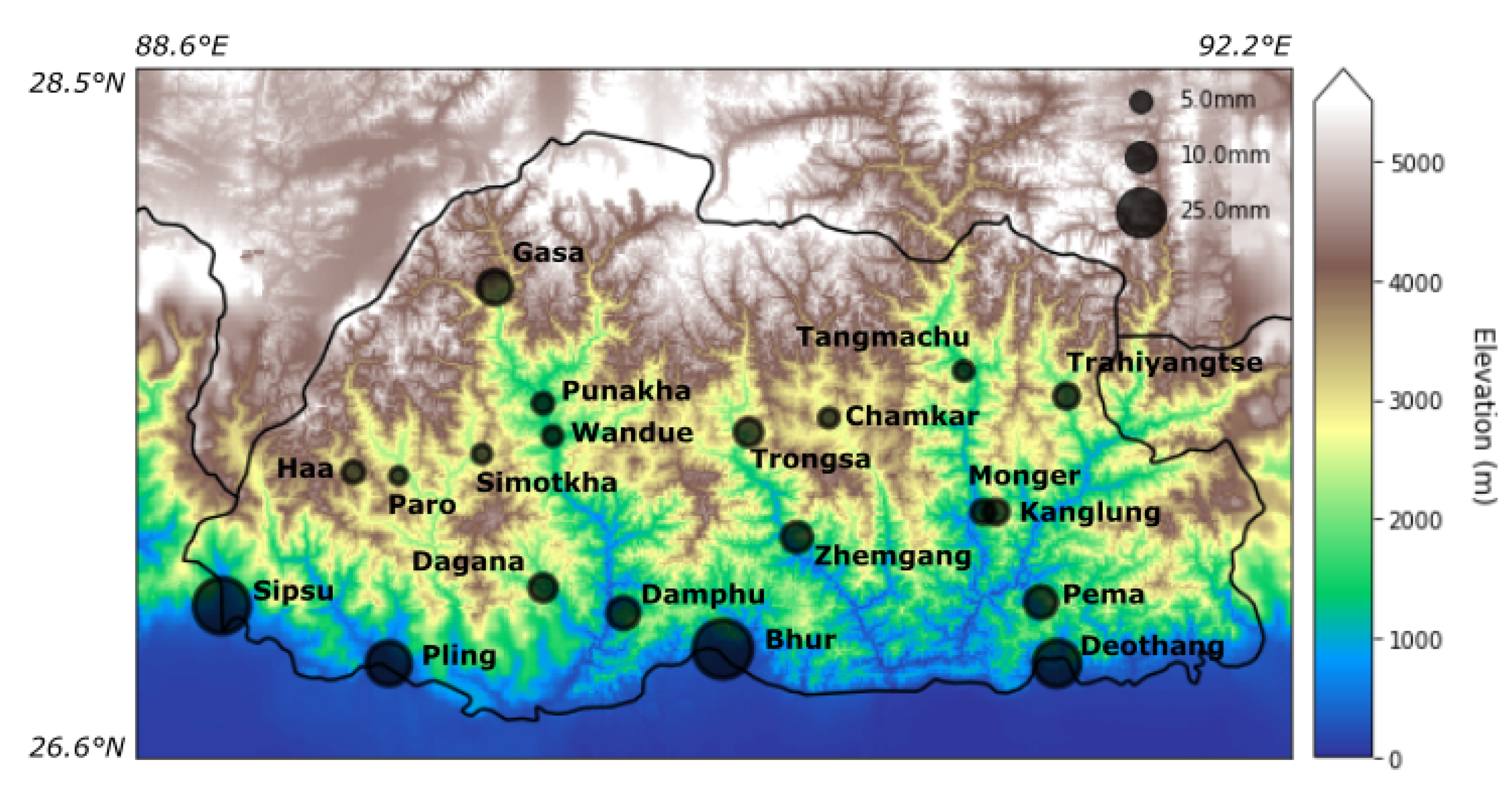
Observational precipitation data were supplied from the Bhutan Hydrological department for 20 weather stations, and the locations of the weather stations are displayed in Figure 1.
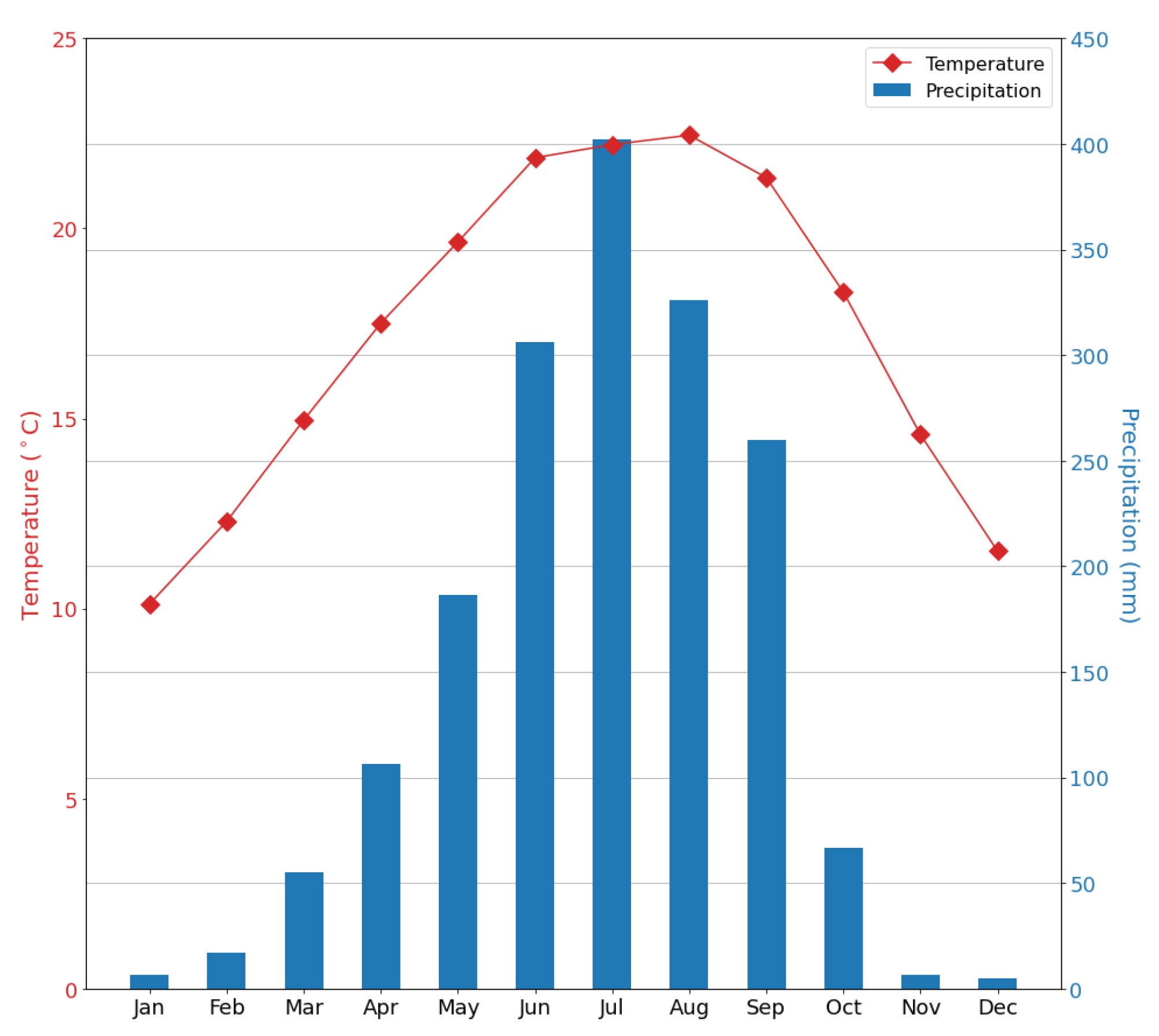
Bhutan is the smallest country in the Hindu Kush Himalaya region, sitting on the eastern slopes of the Himalayas between India and China. The ISM is responsible for 73% of the country’s total rainfall [25], with 60% of the yearly rainfall falling in the monsoon season, June to September (Figure 2). Elevations range from less than 100 m to over 7550 m and the spatial distribution of the monsoon is highly controlled by the varied topography. Bhutan is loosely categorized into four climatic regions depending on precipitation, highest rainfall (3000 to 6000 mm/year) in the southern plains, medium to high (1500 to 2500 mm/year) in the southern High Himalaya region, medium levels (600 to 800 mm/year) in central Bhutan, although these numbers may be double that in windward oriented mountain ranges [26] and absolute precipitation values are lacking in the northern territories.
2.2. Satellite and GPCC Data
The satellite products used are TRMM 3B42 daily data and GPM IMERG V06 (hereafter referred to as GPM). TRMM 3B42 daily data are produced by the joint NASA/Japan Aerospace Exploration Agency (JAXA) Tropical Rainfall Measuring Mission [27]. Data are retrieved at 0.25° × 0.25° resolution over latitude band 35° North to 35° South. The variable total precipitation was used, which represents daily accumulated calibrated surface precipitation combined infrared and microwave, obtained from GES DISC [28]. GPM is provided by the Global Precipitation Mission [29], which was developed as an improvement to the TRMM mission. Data are retrieved at a finer resolution of 0.1° × 0.1° and global coverage has been enlarged to 65° North to 65° South latitudes [30]. The variable precipitationCal was used providing daily accumulated combined microwave IR estimate of precipitation, obtained from GES DISC [28]. The full specifications of the algorithm and data used for GPM are provided by Huffman et al. [31]. The GPCC (Global Precipitation Climatology Centre) product refers to Full Data Monthly V.2020. It contains the monthly land-surface precipitation from rain-Gauges built on GTS-based and Historical Data, based on quality-controlled data from 85,000 stations in GPCC’s data base and is retrieved at 0.25° × 0.25° resolution [32].
2.3. Hadley Sea Surface Temperature Data
Sea surface temperature (SST) data used in this investigation is the monthly version of HadISST sea surface temperature component from The Met Office Hadley Centre [33]. The data provides global coverage and covers the period 1871 to 2018.
2.4. Reanalysis Data Products
The reanalysis product used here is ERA5, a fifth generation reanalysis product from the European Center for Medium-Range Weather Forecasts (ECMWF) for the global climate and weather [34]. It is generated via data assimilation, combining observational data with historical, observationally constrained general circulation model data (GCMs) to produce the best estimate of the global climate state [35]. It is a valuable tool to explore climatic change at local and regional scales as it provides a completed data set and the inclusion of increased satellite observations in the data assimilation of ERA5 strengthen its capabilities in remote regions like Bhutan [36]. The variables used here are total precipitation, vertical integral of divergence of moisture flux, top net thermal radiation, U and V components of wind at 850 hPa, 2 m temperature, and mean sea level pressure. They have a resolution of 0.25° × 0.25°.
3. Data Evaluation: Are Reanalysis Data Suitable to Investigate ISM Change?
To demonstrate the strengths and weaknesses of ERA5 reanalysis in examining ISM change in response to the ENSO and IOD events of 2015/16, it is compared alongside TRMM and GPM satellite products and GPCC precipitation data with local weather station precipitation measurements. The evaluation period is 2012 to 2019, encompassing all the total years of data provided by the weather station measurements.
3.1. Comparing Seasonal Cycle
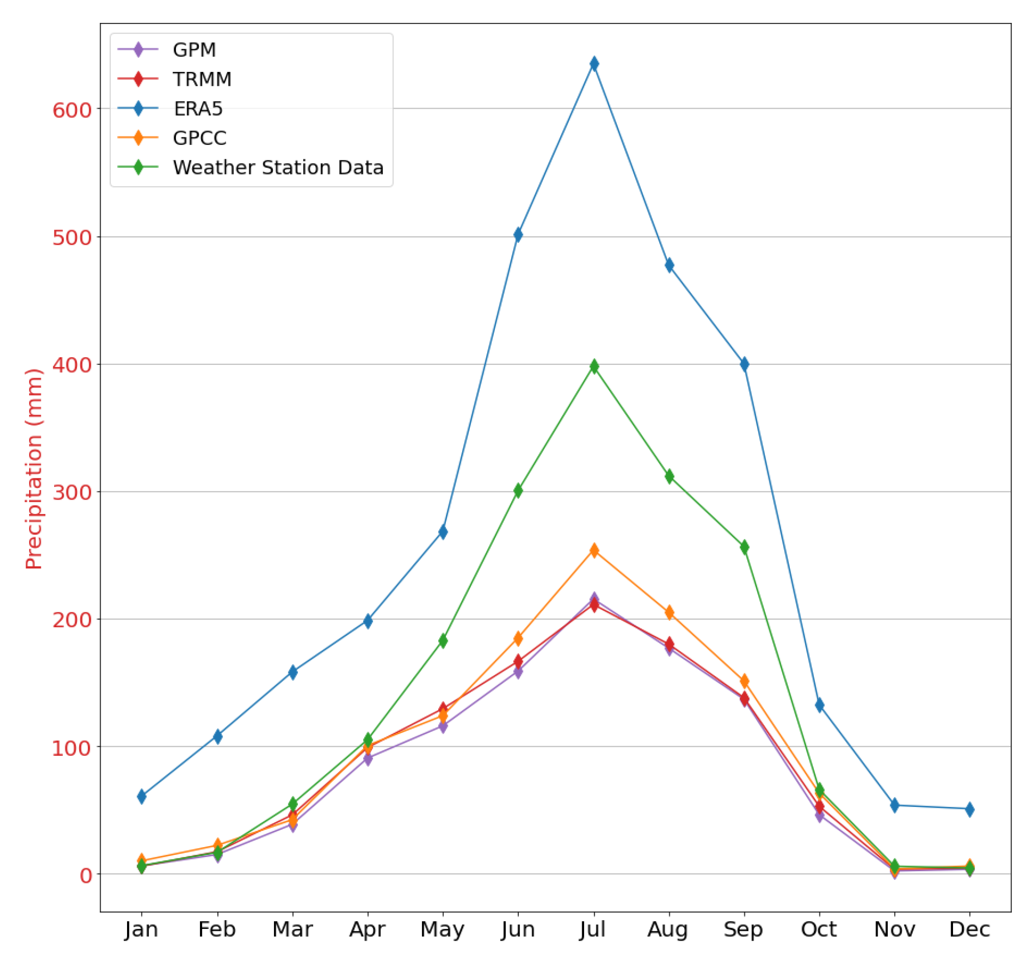
All products reflect the seasonal cycle captured in the weather station data in Figure 3, although there is large variation. Due to the resolution of the data sets when compared to the close placement of the weather stations, an exact regional comparison is not possible. Therefore, the smallest regional that encompasses the weather stations has been taken from the products and the average monthly precipitation calculated for the period 2012 to 2019. This is then compared with the average monthly weather station precipitation. As the focus of this study is monsoon change, the comparison between the data sets is primarily just within the monsoon season of June to September, and no comparison of data products is done for the winter, spring, or autumn months.
ERA5 data overestimate annual precipitation whilst GPM/TRMM and GPCC underestimate. This underestimation by satellite products is consistent with previous studies [37,38] and may be due to errors in satellite sensors or retrieval algorithms [37,39]. Uneven distribution of ground stations, often due to the inadequate number of gauges provided by GPCC, leads to problems with bias correction procedures, further diminishing the accuracy of satellite products and also with the GPCC data [40]. The overestimation of ERA5 is likely due to a prominent wet bias known over the area surrounding the entire foothills of Himalayas [41] and the southern Tibetan Plateau [42,43]. This is likely due to the inability of the coarse spatial resolution of reanalysis data in capturing the intricacy of the Asian summer monsoon and complex surrounding topography.
Concentrating on shape as opposed to values, the sharp peak in monsoon precipitation occurring in July is seen on the ERA5 data in Figure 3. Satellite and GPCC products show a less defined peak with similar values across the monsoon season. This implies that they may not be capturing the true pattern of the monsoon. Various studies have shown TRMM and GPM satellite products to be insufficient when compared with in situ measurements at recording monsoons for various locations including the Tibetan Plateau [44], Thailand [45] and Korea [46]. GPCC has also been shown to be unsuitable to capture extreme events (both wet and dry) over central Asia [47], and therefore may reflect problems capturing monsoon precipitation in complex or remote settings.
3.2. Assessment of Spatial Characteristics
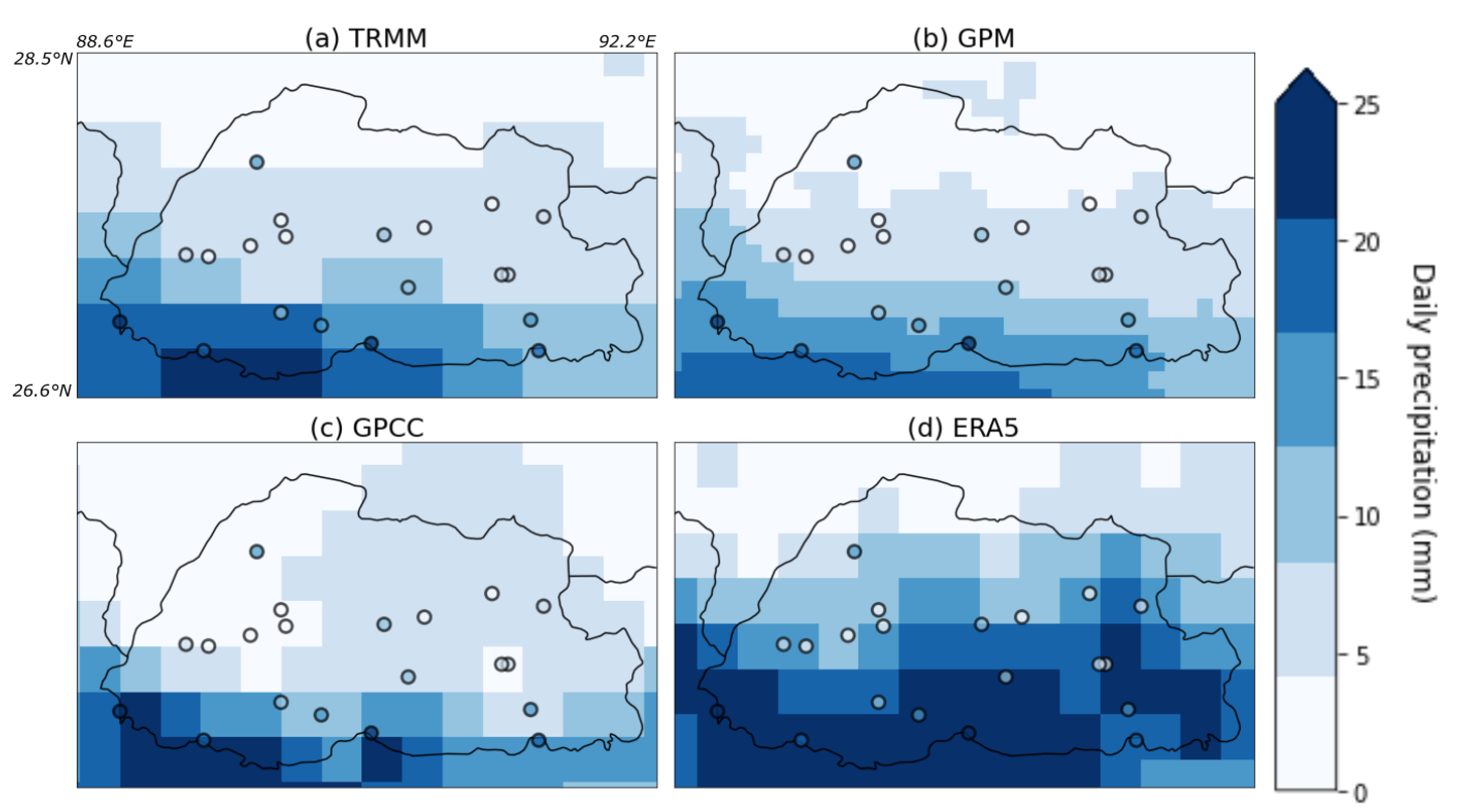
ERA5 and TRMM fit best with the weather station data in the high rainfall area along the southern plains in Figure 4a,d. GPCC records similar levels but only in the southwest (Figure 4c) and GPM underestimates precipitation. This may be due to the satellite’s poor estimation of warm orographic rains as the algorithms of both infrared (IR) or passive microwave (PM) sensors use cloud top temperature thresholds that are too cold to recognize warm orographic clouds. This was illustrated in previous studies over the USA [48] and Ethiopia [49]. In the central region, the satellite products and GPCC are closest to the observed measurements and ERA5 overestimates significantly (Figure 4d). This overestimation by ERA5 may be due again to the above-mentioned wet bias. Gasa is the only station available for comparison in the north and all products underestimate here. Although there is significant overestimation by ERA5, it is the only product to emulate the topography of the region. The two prominent valleys that propagate northward within the central region, identifiable in Figure 1, are only reflected in Figure 4d. These valleys contain slightly higher precipitation amounts than the surrounding mountainous terrain, as well as providing a route for moisture to travel northward. Therefore, they play a significant role in precipitation distribution in Bhutan.
No such pattern is shown from either a satellite product or GPCC, instead showing a movement from high rainfall in the south to low rainfall in the north. This agrees with previous findings that have shown complex and mountainous terrain to be a reoccurring challenge for satellite precipitation estimates [46,49] and for GPCC [42]. It is likely the general assumptions of global satellite products are not accurately representing the specific atmospheric conditions present [30], and GPCC may be over relying on interpolation in remote areas. From the evidence presented here, it is clear that ERA5 reanalysis can reproduce the monsoon peak and is able to capture the effect of Bhutan’s intricate topography on rainfall. However, it has also been highlighted that ERA5 often overestimates the absolute precipitation values. It may be that satellite products and GPCC are closer to actual precipitation values for some regions of our study site. However, due to their limited timespan and lack of variables when compared to ERA5, the reanalysis product may be more appropriate here. Therefore, ERA5 reanalysis is deemed a suitable product to explore monsoon change, but absolute precipitation values may be used with caution.
4. The Regional and Local Impacts of the 2015/2016 ENSO and IOD Events on the ISM—A Bhutan Case Study
4.1. Impact on Monsoon Precipitation
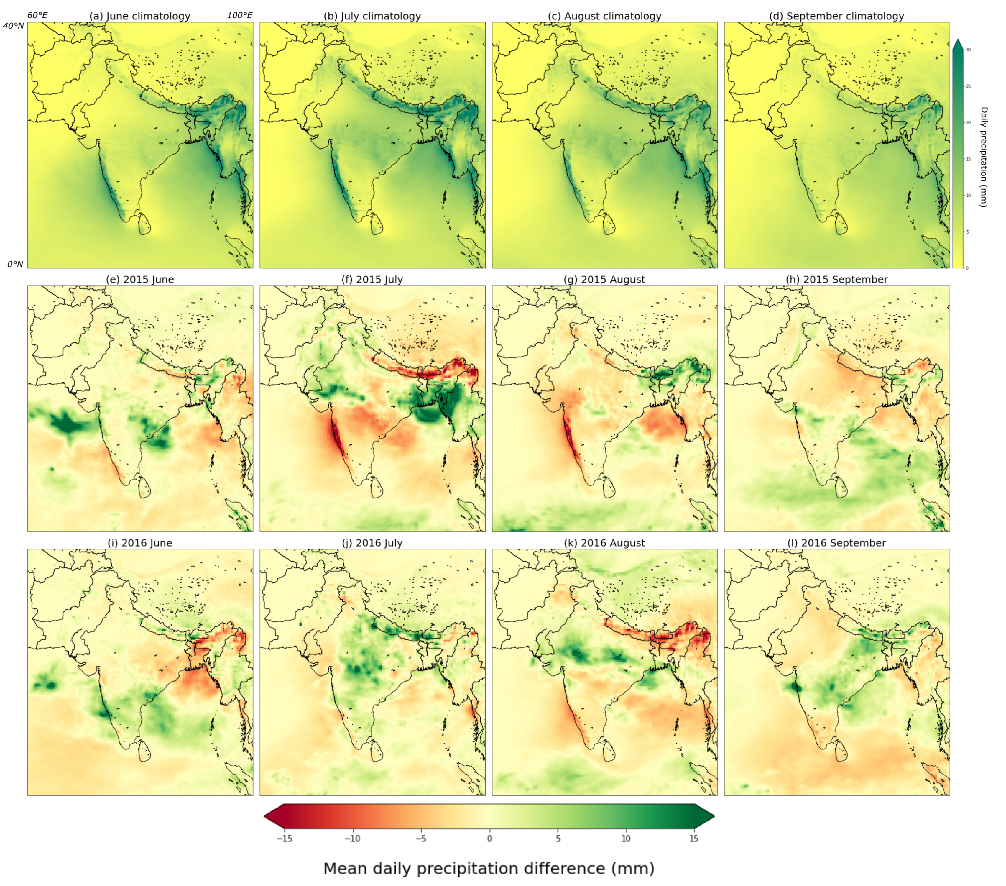
At the regional scale, in 2015, there were large precipitation changes during the peak monsoon months of July and August. In July 2015 (Figure 5f), there is up to 15 mm/day more precipitation than expected over the Bay of Bengal, whilst 15 mm/day less precipitation than expected over India’s west coast, Nepal, Bhutan, and Northern India. The pattern is different, however, in August 2015 with reduced precipitation of up to 5 mm/day over the Bay of Bengal and more precipitation to the north (Figure 5g), whilst reduced rainfall remains over India’s west coast. During the following year, there is disruption to the monsoon onset with a split precipitation pattern across Bhutan (Figure 5i). In July 2016, there is up to 10 mm/day more precipitation than normal across central India, northern India, Nepal, and Bhutan, and no areas of reduced precipitation. However, during August 2016, this is again reversed with now decreased rainfall of up to 10 mm/day in the Nepal/Bhutan area (Figure 5k) but 5–10 mm/day more in central India. In Figure 5l, the region of more precipitation in central India has now spread out, possibly indicating a slower decay of the ISM in September 2016.
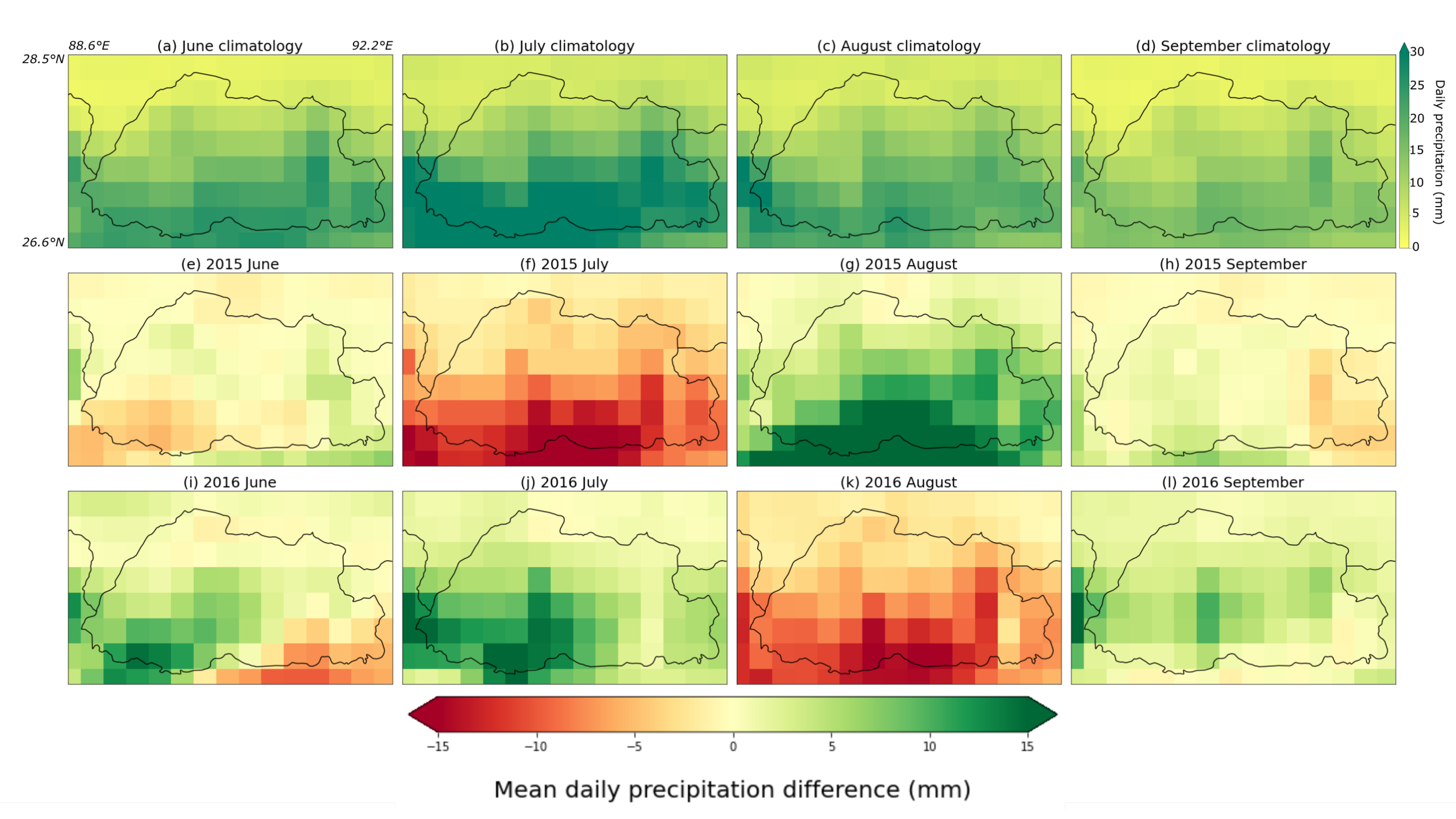
At the local scale, in July 2015 (Figure 6f), there is a reduction in precipitation across the entire country with over 15 mm/day less in the southern areas. However, August 2015 (Figure 6g) shows the inverse, with higher than normal precipitation across the entire country and over 15 mm/day more in the southern plains area and 10 mm/day more in the central valleys. In 2016, there is disruption to the onset with a precipitation split (higher in SW, less in SE) in June (Figure 6i), but then more precipitation than normal over the whole country in July (Figure 6j) with greater than 15 mm/day in the west valley transect. August 2016 (Figure 6k) displays the reverse pattern with a widespread precipitation reduction, most prominent in the southern region with over 15 mm/day less and the southern to central region experiencing between 5 to 10 mm/day less. For the decay of the monsoon in September 2016 (Figure 6l), precipitation is up 7 mm/day more for some central regions.
4.2. Impact on Vertically Integrated Moisture Flux Divergence and Wind at 850 hPa
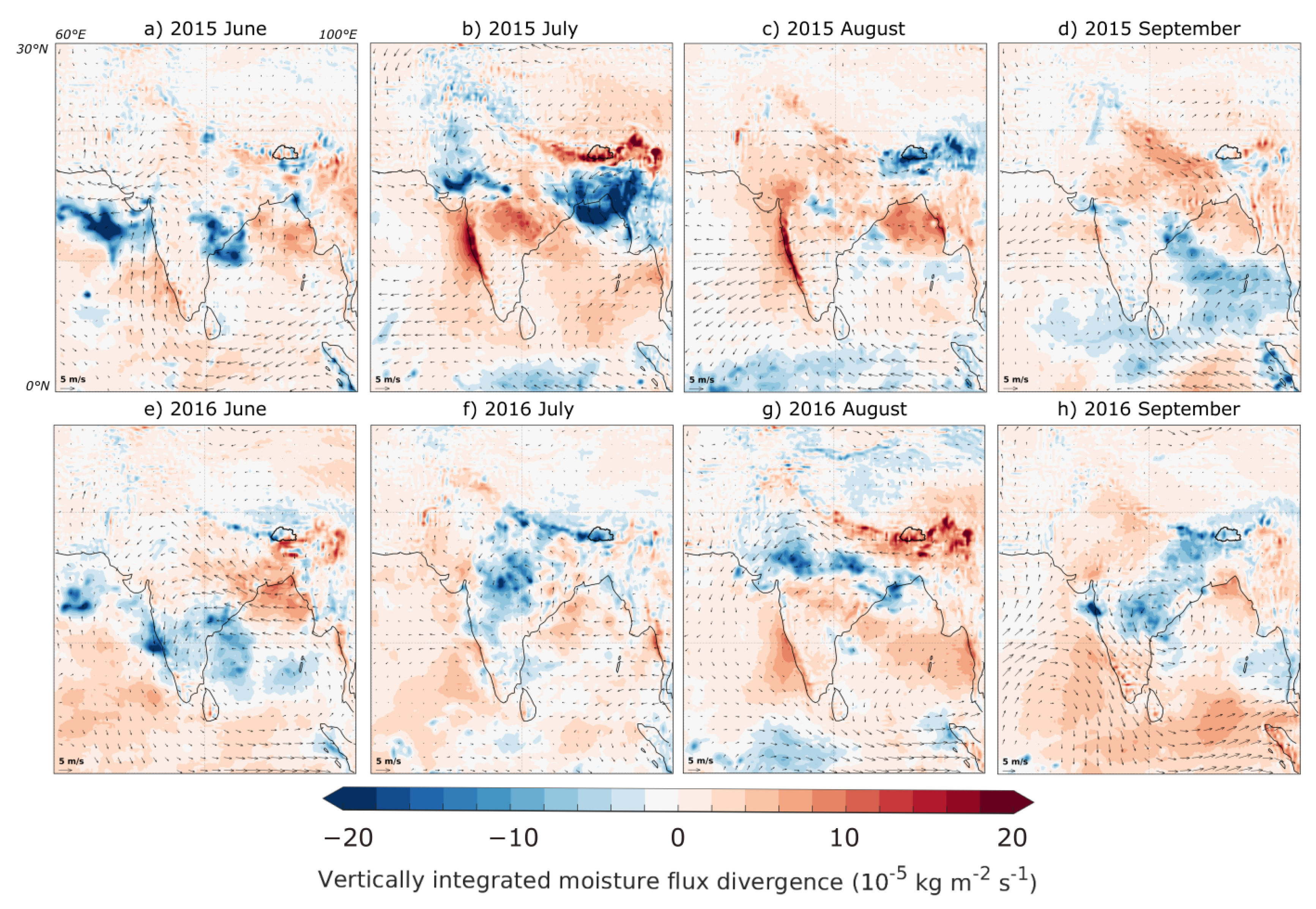
The variables’ vertically integrated moisture flux divergence and wind at 850 hPa are used to explore change to the monsoon flow at the regional scale. The onset of the ISM in 2015 (Figure 7a) is disrupted. The SW monsoon flow has shifted south beneath the Indian peninsula, and little moisture is propagating up to Bhutan. This may reflect a delay to the onset of the ISM. In July (Figure 7b), areas expected to experience moisture convergence are experiencing divergence, indicating that the SW monsoon flow has shifted and air is flowing instead from the high pressure plateau area to the low pressure area over India and the Bay of Bengal. In August 2015 (Figure 7c), the wind pattern reflects a weaker than normal monsoon flow and westerlies, incoming from the Tibetan Plateau, bring moisture to Bhutan creating an area of moisture convergence here. This pattern is unusual as no westerly flow is expected here in August. In 2016, during June (Figure 7e), two opposite areas of moisture flux are meeting in the middle of Bhutan, explaining the precipitation divide. During July 2016 (Figure 7f), there are elements of the normal monsoon flow and more moisture convergence over the border with the Tibetan Plateau, Bhutan, and down into western India. During August 2016, the pattern is again different. Wind is now flowing inland and moisture is diverging over Bhutan and along the border with Tibetan Plateau (Figure 7g). In September 2016 (Figure 7h), moisture is diverging over the Bay of Bengal and moving to India and then spreading up to Bhutan, providing more evidence of a slower ISM decay.
4.3. Temperature and Pressure Gradients during the 2015/16 Monsoon Peaks
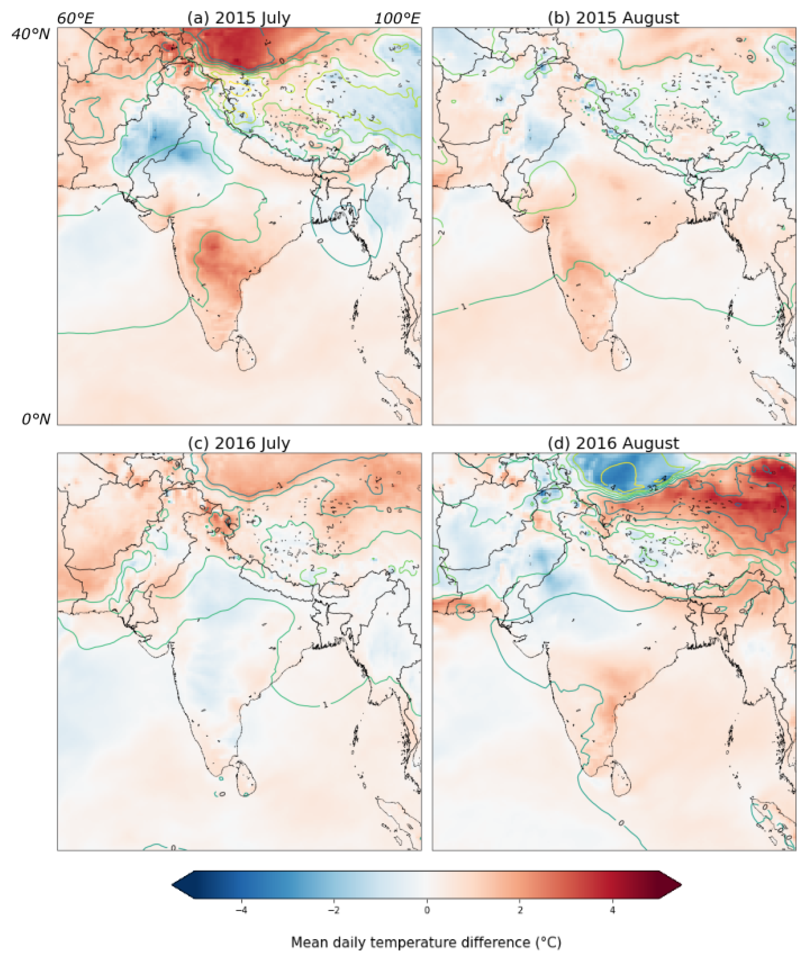
During the normal monsoon season, a south to north temperature pressure gradient is formed due to the warming of the northern Indian Ocean and Indian subcontinent whilst the southern Indian Ocean remains cooler. This causes the monsoon cross equatorial flow [3,50] with winds carrying moisture from the warm Indian Ocean to converge on India’s mountainous west coast, and then on to the Bay of Bengal where the winds turn north and west around India’s low pressure monsoon trough [3,51]. In July 2015, which saw great disruption to the normal moisture and precipitation pattern, there was a higher than normal pressure area over the Tibetan Plateau and a lower than normal pressure area over the Bay of Bengal (Figure 8a). The flow of air from high to low pressure is therefore facilitating the movement of moisture away from Bhutan and taking it south to the Bay of Bengal. This may explain the abnormally low precipitation over Bhutan in July 2015, whilst there was increased precipitation further south. In August 2015, precipitation and moisture variables indicated a return to a more normal monsoon flow, and this is supported by Figure 8b showing slightly higher pressure in the west and lower in the east, maintaining the normal, but weaker, monsoon flow. A closer to normal monsoon flow is also evident in July 2016 (Figure 8c) with pressure marginally lower over central India and the Bay of Bengal when compared to areas to the west and north. During August 2016, which showed strong variance from the normal pattern, a very steep temperature gradient is evident (Figure 8d). There is much higher pressure than normal over regions to the south of the Tibetan Plateau and lower pressure areas over central and west India, which causes the movement of moisture away from the Tibetan plateau, deflecting it from Bhutan and Nepal and carrying it to the low pressure systems over central and west India. This is why a reversed monsoon flow is evident.
5. Discussion
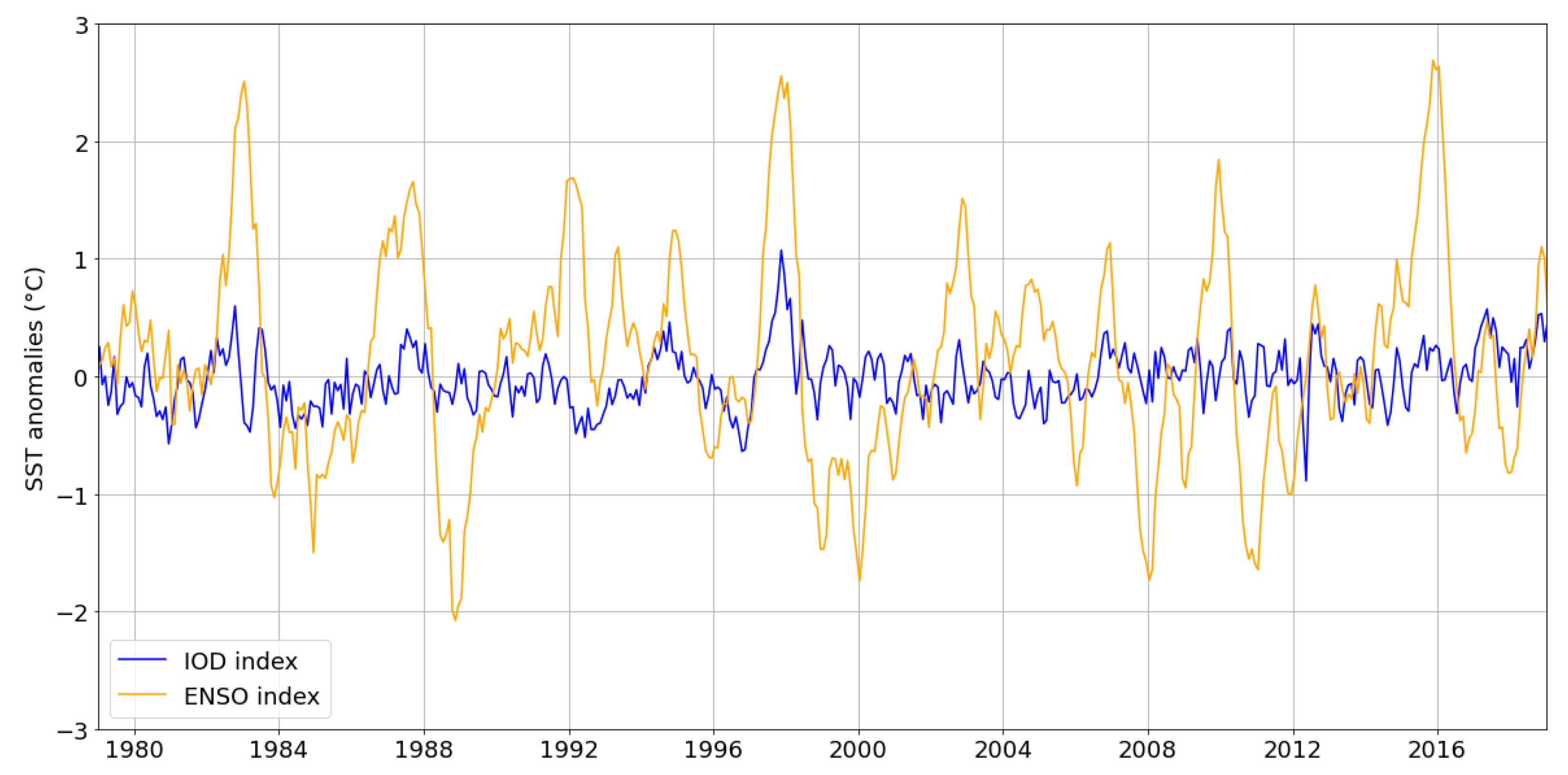
The co-occurrence of a positive IOD and El Niño can incur an anomalously surplus ISM rainfall. This is due to the weakening of the low-level western Pacific divergence center associated with the pure El Niño, which means that a new, anomalous divergence center is created off of Indonesia’s west coast, and an anomalous Walker cell is formed over the IOD region causing the intensification of the cross-equatorial Hadley circulation [4]. By looking for parallels with other simultaneous IOD and ENSO events, event patterns may emerge that could explain some of the impacts experienced during the study period. The 2015/16 El Niño was considered a Super El Niño due to the strength and intensity of its physical forcing [52]. There have been two other Super El Niños recorded: the 1982/83 and 1997/98 events. All reached similar amplitudes based on SST anomalies [53] and all occurred alongside a positive IOD [54] as is shown in Figure 9. However, the events had differing outcomes. During the 1982/83 event, there was a disruption in the inter-annual ISM anomaly, with a deficit in rainfall during the developing year summer monsoon, but a surplus rainfall during the decaying year, likely due to the interplay of the strong positive IOD alongside the strong ENSO [55]. For 1997/98, despite the strong El Niño (as based on the MEI index [56,57], mean monsoon precipitation was 2% above normal [58]. June and September of 1997 had a weakened monsoon circulation, but July and August experienced near normal monsoon precipitation meaning there was no monsoon deficit [59]. This was explained by Slingo and Annamalai [58] to be a result of the suppression of convection over the Maritime Continent and equatorial Indian Ocean leading to a more active TCZ to the north, which subdued the effect of the Walker circulation in June and September, whilst enhancing local Hadley circulation in July and August [58].
For 2015/16, this impact of a surplus ISM was not apparent. There were both periods of drought and increased rainfall across the ISM region, and over the Bhutan study area, a heavily disrupted monsoon in terms of timing rather than rainfall quantity. It may be important to consider whether the lack of the expected behavior is due to the differences in ocean events as compared with those that occurred previously. Some have questioned whether the El Niño was strong enough to be considered “super”. Considering the rapidly rising worldwide decadal scale SST anomalies, including a 0.5 °C rise in tropical Pacific SSTs in the three years leading up to the 2015 event, the SST anomaly amplitude for 2015 is 1 standard deviation lower than during the other super El Niños [60]. Furthermore, the 2015/16 El Niño had a westward shift of SST anomalies when compared to previous events such as 1997/98. This creates unfavorable conditions for positive IOD development [54] as the westward movement of the El Niño causes the rising branch of the walker circulation to shift from the east to the central tropical Pacific, which means the difference in the anomalous walker circulation over the Indian Ocean exhibits a negative IOD like pattern, blocking further development of the positive IOD. From Figure 9, the strength of the positive IOD during 2015/16 is visibly not as great as in 1997/98. Some studies have questioned whether it even constituted a positive IOD. The westward movement of the El Niño caused the rising branch of the walker circulation to shift from the east to the central tropical Pacific. The difference in the anomalous walker circulation over the Indian Ocean then exhibited a negative IOD like pattern, which blocked further development of the positive IOD. This is opposite to what occurred during the 1997/98 event, where the cold SSTs in the eastern Indian ocean maintained the suppression of convection in the region, leading to a positive feedback on enhancing the positive IOD [58].
For the following year, the co-occurrence of a negative IOD and a La Niña may cause an anomalous deficit monsoon situation, due to the reduction of lower level convergence of air over the ISM region [61]. Again, this expected impact of the co-occurrence of these two events in 2016 is hard to distinguish. There was less than normal rainfall over southwest India, supporting previous findings by Sreelekha and Babu [62], but there was also excess rainfall over other regions of the Indian subcontinent. Sreelekha and Babu [62] suggested that this uneven spatial and temporal distribution of rainfall during 2016 was likely to be due to the propagation of monsoon-organized convections (MOC), which were faster over southwest India leading to deficit, but slower with a more sustained presence over the monsoon cloud zone, causing normal monsoon rainfall in other locations. The viability of the events of 2016 can also be questioned in a similar manner to the previous year. When compared with other cold events, the 2016/17 La Niña was comparatively weak, whilst the negative IOD was the strongest in 25 years, driven by a long-term Indian Ocean surface and subsurface warming trend over the last 55 years [15]. This weakness, when compared with other events, is clear in Figure 9. Comparison by Lim and Hendon [15] of the 2016 negative IOD with five previous strong negative IODs; 1992, 1996, 1998, 2005, and 2010, of which only 1988–89, and 2010–11 occurred with a La Niña, showed that only the 1998 event developed in a similar style. This means both events had anomalous ocean subsurface heat accumulating in the tropical western Indian Ocean and a surface westerly wind burst in the tropical central Indian Ocean, but with weaker magnitudes in 1998 than 2016. In 2016, with one weak and one strong event, can the impact on the ISM during be the result of the co-occurrence of two ocean phenomena or rather the dominance of a negative IOD? However, a lesser ISM, the expected impact of a negative IOD acting alone, was only recorded in some areas during August and was preceded by a rainfall surplus during July 2016. Therefore, the extent of influence of the IOD and ENSO during this period is unclear.
As well as questioning the viability of the ocean events, the weakening of the relationship between ENSO and the ISM [5] may also be the reason why the expected impacts of the co-occurrence of the two ocean phenomena did not occur. Other drivers of interannual variability of the monsoon must therefore be considered, such as varying boundary conditions. This includes changing SST anomalies over the equatorial Pacific and Indian oceans [63], or winter pressure anomalies due to changes of Eurasian snow cover changes [64,65]. The SSTs of the North Atlantic also have an influence on the ISM via the Atlantic Multi-decadal Oscillation (AMO) [66,67]. This produces a continued weakening (strengthening) of the tropospheric temperature meridional gradient by encouraging a negative (positive) tropospheric temperature anomaly over Eurasia in the late boreal summer to autumn. This leads to an early (late) SW monsoon withdrawal and decrease (increase) of seasonal rainfall. The Pacific Decadal Oscillation (PDO), which describes the SST variability occurring over 20 to 30 years in the mid latitudes of the Pacific Ocean [68], can affect the interannual variability of the monsoon rainfall through the Walker circulation associated with ENSO [69]. The PDO positive phase can strengthen the eastward migration of the ascending branch of the Walker circulation associated with El Niño conditions. This causes reduced convection over India during the monsoon and prevents the ascent of air over the Indian subcontinent leading to a higher pressure zone with reduced cloud formation [70]. When ENSO and the PDO are in phase (out of phase), then the resulting ENSO anomalies are intensified (dampened) and may expand (reduce) poleward [42], meaning the warm phase of the PDO is negatively correlated to precipitation in central and southern India [71,72], and there are more severe El Niño induced droughts during the warm phase of the PDO. Currently, we are in a positive phase of the PDO, so ENSO induced subsidence is more likely to be enhanced and the impact of La Niña reduced [72]. ENSO induced subsidence was possibly enhanced for July 2015 and the associated wetter impacts of La Niña were possibly subdued during August 2016 over Bhutan, yet there is no definite impact from which to draw a conclusion that the PDO was causing this.
It is also important to consider that much of the ISM interannual variability is driven by the internal dynamics involved, operating chaotically [59,69]. For the 1997/98 ENSO event, the more clearly definable surplus ISM was explained by some to be the result of the strong positive dipole that was taking place simultaneously [4], but others stated that it was likely the accidental behavior of an inherently noisy monsoon system [73]. Considering that the impacts witnessed over 2015/16 are much more turbulent and harder to define when compared with a more clear cut event like that of 1997/98, it may be that the events of 2015/16 are the product of a chaotic monsoon system influenced by numerous drivers of internal variability.
At the local scale, drivers of monsoon variability are further amplified/modified by tectonic and orographic processes. Within Bhutan tectonic processes are the primary control on moisture migration [74], facilitating movement through the deeply incised valleys to the dry Tibetan Plateau. The split precipitation pattern over Bhutan seen in September 2015 and June 2016 (Figure 6) is likely the product of local topography. The Shillong Plateau, the most prominent orographic barrier in the south Himalayas [74], sits to the south of Bhutan and creates an orographic rain shadow in east Bhutan, whilst the low elevations of the Sankosh valley in the west enhances precipitation. This may explain the divided precipitation seen. The strong control of Bhutan’s topography seems to amplify the alterations to the ISM already occurring at a larger scale. If moisture is diverging over the country, the most reduced precipitation is found in the deeply incised valleys then compared to the surrounding areas, whereas, if moisture is converging over the country, the greatest precipitation occurs in the low lying southern area found before the sharp rise in topography and the presence of the Himalayan orographic barrier. Therefore, it is likely that disruption to the ISM at a local scale was the product of numerous drivers of ISM variability alongside ENSO and IOD, but these are further amplified and/or modified by the intricate topography and orographic processes. For this reason, a direct link between ENSO and IOD activity and changes to the monsoon over Bhutan is hard to distinguish.
6. Conclusions
This study aimed to explore how the ISM was affected at local and regional scales during the 2015 to 2016 period in relation to the ongoing ENSO and IODs. There was clear disruption to the ISM during the study period. In 2015, the monsoon onset was delayed, and the entire monsoon flow shifted during July. This caused rain deficits over Bhutan, Nepal, and central India and rain surpluses over the Bay of Bengal and surrounding area. In August, the monsoon returned to a normal albeit weaker monsoon flow. During 2016, the monsoon season onset was disrupted with a southeast/northwest split precipitation pattern. During July, there was a close to normal monsoon flow rain with surplus over central India, Nepal, and Bhutan; however, in August, there was a reversed monsoon flow. Moisture was instead moved away from the southern Himalayan front and transported inland to northern India, and there was a slow monsoon decay in September.
Whilst it is possible to attribute some of these regional scale changes to the ENSO and IOD events, the expected impacts of simultaneous ENSO and IOD events are hard to recognize. This may be due to the viability of the 2015/16 ENSO and IOD events or it could also be related to the supposed weakening of the ENSO/ISM relationship. ENSO cannot explain the full scale of changes that occur to monsoons, and it is likely that the 2015/16 monsoon disruption was driven by a combination of factors alongside ENSO and the IOD, including varying boundary conditions (such as changes to SST anomalies and Eurasian snow cover), the Pacific Decadal Oscillation (PDO), the Atlantic Multi-decadal Oscillation (AMO), and internal chaotic variability. This plethora of factors, interacting and influencing one another, make defining direct impacts of ENSO on the ISM increasingly difficult. Taking into account the multitude of drivers of monsoon variability acting on the ISM at a regional level, distinguishing direct ENSO/IOD consequences on a local level over Bhutan is even more difficult due to the role of topography further altering the already disrupted monsoon.
Bhutan’s dependency on agriculture and natural resources makes the country eminently vulnerable to ISM spatial-temporal variability. With over 60% employed in the agricultural sector [75] and an estimated economic potential of over 100 million US$ in annual revenue [76] from its recently developed hydropower industry, disruption to the monsoon has severe repercussions. Alterations to the onset or offset, as was seen in 2015/16, has a direct negative affect on both subsistence farming and cash crop yields, whilst changes to monsoon precipitation patterns across the high altitude Himalayan regions increase the risk of flash flooding, landslides, and further diminishing Himalayan glacier extent, which has long-term repercussions on Asia’s water resources and therefore hydropower [77]. It is largely unclear how global monsoon variability will change in the future. Multimodel ensemble projections from CMIP6 indicate that northern hemisphere monsoon rainfall will likely increase under a warming climate [78] and that late withdrawals of the monsoon may be more common [79]. There is more ambiguity surrounding how ENSO and IOD events will change under future climate scenarios, as while one or even several of the processes that dictate the characteristics of an ENSO event may be altered by climate change, whether this will lead to enhanced, dampened, more frequent, or more intense ENSO activity is unclear [80]. Despite this lack of clarity, it is likely there will be a more unpredictable monsoon climate over Bhutan in the future. Considering the country’s inherent vulnerability to climatic change, the threat of a future unpredictable monsoon climate will have severe repercussions for Bhutan, unless mitigation measures are rapidly employed.
Author Contributions
Conceptualization, K.P., Q.Z., and J.A.; methodology, K.P. and J.A.; formal analysis, K.P.; investigation, K.P.; resources, Q.Z., J.A., N.W., and K.P.; data curation, Q.Z., J.A., and N.W.; writing—original draft preparation, K.P.; writing—review and editing, K.P., J.A., and Q.Z.; visualization, K.P. and J.A.; supervision, Q.Z. and J.A.; project administration, Q.Z. and J.A. All authors have read and agreed to the published version of the manuscript.
Funding
This work was supported by the Swedish Research Council (Vetenskapsrådet, Grant No. 2013-06476).
Data Availability Statement
GPM IMERG V06: DOI 10.5067/GPM/IMERGDF/DAY/06; TRMM 3B42: DOI 10.5067/TRMM/TMPA/DAY/7; GPCC: DOI 10.5676/DWDGPCC/FDMV2020025; Hadley SST: DOI 10.1029/2002JD002670; ERA5: DOI 10.24381/CDS.F17050D7.
Acknowledgments
The data analysis was performed using resources provided by the Swedish National Infrastructure for Computing (SNIC) at the National Supercomputer Centre (NSC), which is partially funded by the Swedish Research Council through Grant No. 2018-05973.
Conflicts of Interest
The authors declare no conflict of interest.
References
- Wang, P.X.; Wang, B.; Cheng, H.; Fasullo, J.; Guo, Z.; Kiefer, T.; Liu, Z. The global monsoon across time scales: Mechanisms and outstanding issues. Earth-Sci. Rev. 2017, 174, 84–121. [Google Scholar] [CrossRef]
- Singh, D.; Ghosh, S.; Roxy, M.K.; McDermid, S. Indian summer monsoon: Extreme events, historical changes, and role of anthropogenic forcings. WIREs Clim. Chang. 2019, 10, e571. [Google Scholar] [CrossRef]
- Goswami, B.; Chakravorty, S. Dynamics of the Indian Summer Monsoon Climate; Oxford University Press: Oxford, UK, 2017; Volume 1. [Google Scholar] [CrossRef]
- Ashok, K.; Guan, Z.; Saji, N.H.; Yamagata, T. Individual and Combined Influences of ENSO and the Indian Ocean Dipole on the Indian Summer Monsoon. J. Clim. 2004, 17, 3141–3155. [Google Scholar] [CrossRef]
- Kumar, K.K.; Rajagopalan, B.; Cane, M.A. On the Weakening Relationship Between the Indian Monsoon and ENSO. Science 1999, 284, 2156–2159. [Google Scholar] [CrossRef] [Green Version]
- Cook, E.R.; Anchukaitis, K.J.; Buckley, B.M.; D’Arrigo, R.D.; Jacoby, G.C.; Wright, W.E. Asian Monsoon Failure and Megadrought During the Last Millennium. Science 2010, 328, 486–489. [Google Scholar] [CrossRef] [PubMed] [Green Version]
- Mishra, V.; Smoliak, B.V.; Lettenmaier, D.P.; Wallace, J.M. A prominent pattern of year-to-year variability in Indian Summer Monsoon Rainfall. Proc. Natl. Acad. Sci. USA 2012, 109, 7213–7217. [Google Scholar] [CrossRef] [Green Version]
- Lau, G.C.; Wang, G. Interactions between the Asian monsoon and the El Niño Southern Oscillation. In The Asian Monsoon; Springer-Praxis: Chichester, UK, 2006. [Google Scholar]
- Lau, K.M.; Wu, H.T. Assessment of the impacts of the 1997–98 El Niño on the Asian-Australia Monsoon. Geophys. Res. Lett. 1999, 26, 1747–1750. [Google Scholar] [CrossRef]
- Gadgil, S.; Vinayachandran, P.N.; Francis, P.A.; Gadgil, S. Extremes of the Indian summer monsoon rainfall, ENSO and equatorial Indian Ocean oscillation: EXTREMES OF INDIAN SUMMER MONSOON RAINFALL. Geophys. Res. Lett. 2004, 31. [Google Scholar] [CrossRef] [Green Version]
- Behera, S.K.; Ratnam, J.V. Quasi-asymmetric response of the Indian summer monsoon rainfall to opposite phases of the IOD. Sci. Rep. 2018, 8, 123. [Google Scholar] [CrossRef]
- Ummenhofer, C.C.; Sen Gupta, A.; Li, Y.; Taschetto, A.S.; England, M.H. Multi-decadal modulation of the El Niño–Indian monsoon relationship by Indian Ocean variability. Environ. Res. Lett. 2011, 6, 034006. [Google Scholar] [CrossRef]
- Stockdale, T.; Balmaseda, M.; Ferranti, L. The 2015/2016 El Niño and beyond. ECMWF 2017, 151. [Google Scholar] [CrossRef]
- Avia, L.Q.; Sofiati, I. Analysis of El Niño and IOD Phenomenon 2015/2016 and Their Impact on Rainfall Variability in Indonesia. IOP Conf. Ser. Earth Environ. Sci. 2018, 166, 012034. [Google Scholar] [CrossRef] [Green Version]
- Lim, E.P.; Hendon, H.H. Causes and Predictability of the Negative Indian Ocean Dipole and Its Impact on La Niña during 2016. Sci. Rep. 2017, 7, 12619. [Google Scholar] [CrossRef] [PubMed] [Green Version]
- Saji, N.H.; Goswami, B.N.; Vinayachandran, P.N.; Yamagata, T. A dipole mode in the tropical Indian Ocean. Nature 1999, 401, 360–363. [Google Scholar] [CrossRef] [PubMed]
- Thomalla, F.; Boyland, M.; Jegillos, S.; Sharma, R.; Shairi, M.; Bonapace, T.; Rafisura, S.; Sarkar, K.; Madhurima, H. Enhancing Resilience to Extreme Climate Events: Lessons from the 2015–2016 El Niño Event in Asia and the Pacific A Multi-Agency Study of Lessons Learnt; Technical Report; UNDP: New York, NY, USA, 2017. [Google Scholar]
- Shrestha, U.B.; Gautam, S.; Bawa, K.S. Widespread Climate Change in the Himalayas and Associated Changes in Local Ecosystems. PLoS ONE 2012, 7, e36741. [Google Scholar] [CrossRef] [Green Version]
- Sovacool, B.K.; D’Agostino, A.L.; Meenawat, H.; Rawiani, A. Expert views of climate change adaptation in least developed Asia. J. Environ. Manag. 2012, 97, 78–88. [Google Scholar] [CrossRef]
- Hamm, A.; Arndt, A.; Kolbe, C.; Wang, X.; Thies, B.; Boyko, O.; Reggiani, P.; Scherer, D.; Bendix, J.; Schneider, C. Intercomparison of Gridded Precipitation Datasets over a Sub-Region of the Central Himalaya and the Southwestern Tibetan Plateau. Water 2020, 12, 3271. [Google Scholar] [CrossRef]
- Gao, Y.; Xiao, L.; Chen, D.; Xu, J.; Zhang, H. Comparison between past and future extreme precipitations simulated by global and regional climate models over the Tibetan Plateau: Downscaled Extreme Precipitations Simulation over the Tibet. Int. J. Climatol. 2018, 38, 1285–1297. [Google Scholar] [CrossRef]
- Mahto, S.S.; Mishra, V. Does ERA-5 Outperform Other Reanalysis Products for Hydrologic Applications in India? J. Geophys. Res. Atmos. 2019, 124, 9423–9441. [Google Scholar] [CrossRef]
- Gleixner, S.; Demissie, T.; Diro, G.T. Did ERA5 Improve Temperature and Precipitation Reanalysis over East Africa? Atmosphere 2020, 11, 996. [Google Scholar] [CrossRef]
- IRI. WORLDBATH: ETOPO5 5x5 minute Navy Bathymetry. 2015. Available online: http://iridl.ldeo.columbia.edu/SOURCES/.WORLDBATH/ (accessed on 20 October 2020).
- Dorji, U.; Olesen, J.E.; Bøcher, P.K.; Seidenkrantz, M.S. Spatial Variation of Temperature and Precipitation in Bhutan and Links to Vegetation and Land Cover. Mt. Res. Dev. 2016, 36, 66–79. [Google Scholar] [CrossRef] [Green Version]
- Eguchi, T. Synoptic and Local Analysis of Relationship between Climate and Forest in the Bhutan Himalaya (Preliminary Report); Technical Report; Research and Development Centre Yusipang, Department of Forest and Park Services, Ministry of Agriculture and Forest: Bhutan, Thimpu, 2011.
- Huffman, G.J.; Bolvin, D.T.; Nelkin, E.J.; Adler, R.F. TRMM (TMPA) Precipitation L3 1 day 0.25 degree x 0.25 degree V7. 2016. Type: Dataset. Available online: https://doi.org/10.5067/TRMM/TMPA/DAY/7 (accessed on 10 November 2020).
- NASA. GES DISC. 2020. Available online: https://disc.gsfc.nasa.gov (accessed on 15 September 2020).
- Huffman, G.J.; Stocker, E.F.; Bolvin, D.T.; Tan, J. GPM IMERG Final Precipitation L3 1 day 0.1 degree x 0.1 degree V06. 2019. Type: Dataset. Available online: https://doi.org/10.5067/GPM/IMERGDF/DAY/06 (accessed on 15 September 2020).
- Kukulies, J.; Chen, D.; Wang, M. Temporal and spatial variations of convection, clouds and precipitation over the Tibetan Plateau from recent satellite observations. Part II: Precipitation climatology derived from global precipitation measurement mission. Int. J. Climatol. 2020, 40, 4858–4875. [Google Scholar] [CrossRef]
- Huffman, G.J.; Bolvin, D.T.; Braithwaite, D.; Hsu, K.; Joyce, R.; Xie, P.; Yoo, S.H. IMERG: Integrated Multi-satellitE Retrievals for GPM|NASA Global Precipitation Measurement Mission. 2015. Available online: https://disc.gsfc.nasa.gov/datasets/GPM_3IMERGDF_06/summary (accessed on 15 September 2020).
- Schneider, U.; Becker, A.; Finger, P.; Rustemeier, E.; Ziese, M. GPCC Full Data Monthly Version 2020 at 0.25°: Monthly Land-Surface Precipitation from Rain-Gauges Built on GTS-Based and Historic Data: Gridded Monthly Totals. 2020. Type: Dataset. Available online: https://doi.org/10.5676/DWD_GPCC/FD_M_V2020_025 (accessed on 5 February 2021).
- Rayner, N.A.; Parker, D.E.; Horton, E.B.; Folland, C.K.; Alexander, L.V.; Rowell, D.P.; Kent, E.C.; Kaplan, A. Global analyses of sea surface temperature, sea ice, and night marine air temperature since the late nineteenth century. J. Geophys. Res. 2003, 108, 4407. [Google Scholar] [CrossRef]
- Hersbach, H.; Dee, D. ERA5 reanalysis is in production. ECMWF Newsl. 2016, 147. [Google Scholar] [CrossRef]
- Priestley, M.D.K.; Ackerley, D.; Catto, J.L.; Hodges, K.I.; McDonald, R.E.; Lee, R.W. An Overview of the Extratropical Storm Tracks in CMIP6 Historical Simulations. J. Clim. 2020, 33, 6315–6343. [Google Scholar] [CrossRef]
- Copernicus Climate Change Service. ERA5 Monthly Averaged Data on Single Levels from 1979 to Present. 2019. Type: Dataset. Available online: https://doi.org/10.24381/CDS.F17050D7 (accessed on 11 January 2020).
- Jiang, Q.; Li, W.; Wen, J.; Qiu, C.; Sun, W.; Fang, Q.; Xu, M.; Tan, J. Accuracy Evaluation of Two High-Resolution Satellite-Based Rainfall Products: TRMM 3B42V7 and CMORPH in Shanghai. Water 2018, 10, 40. [Google Scholar] [CrossRef] [Green Version]
- Mehran, A.; AghaKouchak, A. Capabilities of satellite precipitation datasets to estimate heavy precipitation rates at different temporal accumulations. Hydrol. Process. 2014, 28, 2262–2270. [Google Scholar] [CrossRef]
- Shen, Y.; Xiong, A.; Wang, Y.; Xie, P. Performance of high-resolution satellite precipitation products over China. J. Geophys. Res. Atmos. 2010, 115. [Google Scholar] [CrossRef]
- Krishna, U.V.M.; Das, S.K.; Deshpande, S.M.; Doiphode, S.L.; Pandithurai, G. The assessment of Global Precipitation Measurement estimates over the Indian subcontinent. Earth Space Sci. 2017, 4, 540–553. [Google Scholar] [CrossRef]
- Singh, T.; Saha, U.; Prasad, V.; Gupta, M.D. Assessment of newly-developed high resolution reanalyses (IMDAA, NGFS and ERA5) against rainfall observations for Indian region. Atmos. Res. 2021, 259, 105679. [Google Scholar] [CrossRef]
- Wang, Y.; Yang, K.; Pan, Z.; Qin, J.; Chen, D.; Lin, C.; Chen, Y.; Tang, W.; Han, M.; Lu, N.; et al. Evaluation of Precipitable Water Vapor from Four Satellite Products and Four Reanalysis Datasets against GPS Measurements on the Southern Tibetan Plateau. J. Clim. 2017, 30, 5699–5713. [Google Scholar] [CrossRef]
- Gao, Y.; Xu, J.; Chen, D. Evaluation of WRF Mesoscale Climate Simulations over the Tibetan Plateau during 1979–2011. J. Clim. 2015, 28, 2823–2841. [Google Scholar] [CrossRef] [Green Version]
- Xu, R.; Tian, F.; Yang, L.; Hu, H.; Lu, H.; Hou, A. Ground validation of GPM IMERG and TRMM 3B42V7 rainfall products over southern Tibetan Plateau based on a high-density rain gauge network: Validation of GPM and TRMM Over TP. J. Geophys. Res. Atmos. 2017, 122, 910–924. [Google Scholar] [CrossRef]
- Chokngamwong, R.; Chiu, L.S. Thailand Daily Rainfall and Comparison with TRMM Products. J. Hydrometeorol. 2008, 9, 256–266. [Google Scholar] [CrossRef]
- Kim, K.; Park, J.; Baik, J.; Choi, M. Evaluation of topographical and seasonal feature using GPM IMERG and TRMM 3B42 over Far-East Asia. Atmos. Res. 2017, 187, 95–105. [Google Scholar] [CrossRef]
- Hu, Z.; Zhou, Q.; Chen, X.; Li, J.; Li, Q.; Chen, D.; Liu, W.; Yin, G. Evaluation of three global gridded precipitation data sets in central Asia based on rain gauge observations. Int. J. Climatol. 2018, 38, 3475–3493. [Google Scholar] [CrossRef]
- Sungmin, O.; Kirstetter, P.E. Evaluation of diurnal variation of GPM IMERG-derived summer precipitation over the contiguous US using MRMS data. Q. J. R. Meteorol. Soc. 2018, 144, 270–281. [Google Scholar] [CrossRef] [Green Version]
- Dinku, T.; Chidzambwa, S.; Ceccato, P.; Connor, S.J.; Ropelewski, C.F. Validation of high resolution satellite rainfall products over complex terrain. Int. J. Remote Sens. 2008, 29, 4097–4110. [Google Scholar] [CrossRef]
- Sørland, S.L.; Sorteberg, A.; Liu, C.; Rasmussen, R. Precipitation response of monsoon low-pressure systems to an idealized uniform temperature increase. J. Geophys. Res. Atmos. 2016, 121, 6258–6272. [Google Scholar] [CrossRef] [Green Version]
- Gadgil, S. The Indian Monsoon 4. Links to Cloud Systems over the Tropical Oceans. Resonance 2008, 13, 218–235. [Google Scholar] [CrossRef]
- Rupic, M.; Wetzell, L.; Marra, J.J.; Balwani, S. 2014–2016 El Niño Assessment Report An Overview of the Impacts of the 2014–16 El Niño on the U.S.—Affiliated Pacific Islands (USAPI); Technical Report; National Oceanic and Atmospheric Administration, NOAA National Centers for Environmental Information (NCEI): Honolulu, HI, USA, 2018.
- Xue, Y.; Kumar, A. Evolution of the 2015/16 El Niño and historical perspective since 1979. Sci. China Earth Sci. 2017, 60, 1572–1588. [Google Scholar] [CrossRef] [Green Version]
- Liu, L.; Yang, G.; Zhao, X.; Feng, L.; Han, G.; Wu, Y.; Yu, W. Why Was the Indian Ocean Dipole Weak in the Context of the Extreme El Niño in 2015? J. Clim. 2017, 30, 4755–4761. [Google Scholar] [CrossRef]
- Chaudhuri, S.; Pal, J. The influence of El Niño on the Indian summer monsoon rainfall anomaly: A diagnostic study of the 1982/83 and 1997/98 events. Meteorol. Atmos. Phys. 2014, 124, 183–194. [Google Scholar] [CrossRef]
- Wolter, K.; Timlin, M.S. Monitoring ENSO in COADS with a seasonally adjusted principal component index. In Proceedings of the 17th Climate Diagnostics Workshop; NOAA/NMC/CAC, NSSL, Oklahoma Climate Survey; CIMMS and the School of Meteorology, University of Oklahoma: Norman, OK, USA, 1993; pp. 52–57. [Google Scholar]
- Wolter, K.; Timlin, M.S. Measuring the strength of ENSO events: How does 1997/98 rank? Weather 1998, 53, 315–324. [Google Scholar] [CrossRef]
- Slingo, J.M.; Annamalai, H. 1997: The El Niño of the Century and the Response of the Indian Summer Monsoon. Mon. Weather Rev. 2000, 128, 1778–1797. [Google Scholar] [CrossRef]
- Cherchi, A.; Navarra, A. Influence of ENSO and of the Indian Ocean Dipole on the Indian summer monsoon variability. Clim. Dyn. 2013, 41, 81–103. [Google Scholar] [CrossRef] [Green Version]
- Hameed, S.N.; Jin, D.; Thilakan, V. A model for super El Niños. Nat. Commun. 2018, 9, 2528. [Google Scholar] [CrossRef]
- Krishnamurti, T.N.; Bedi, H.S.; Subramaniam, M. The Summer Monsoon of 1987. J. Clim. 1989, 2, 321–340. [Google Scholar] [CrossRef] [Green Version]
- Sreelekha, P.N.; Babu, C.A. Is the negative IOD during 2016 the reason for monsoon failure over southwest peninsular India? Meteorol. Atmos. Phys. 2019, 131, 413–420. [Google Scholar] [CrossRef]
- Rajeevan, M. Winter surface pressure anomalies over Eurasia and Indian summer monsoon. Geophys. Res. Lett. 2002, 29, 94-1–94-4. [Google Scholar] [CrossRef]
- Blanford, H.F., II. On the connexion of the Himalaya snowfall with dry winds and seasons of drought in India. Proc. R. Soc. Lond. 1884, 37, 3–22. [Google Scholar] [CrossRef]
- Bamzai, A.S.; Shukla, J. Relation between Eurasian Snow Cover, Snow Depth, and the Indian Summer Monsoon: An Observational Study. J. Clim. 1999, 12, 3117–3132. [Google Scholar] [CrossRef]
- Goswami, B.N.; Madhusoodanan, M.S.; Neema, C.P.; Sengupta, D. A physical mechanism for North Atlantic SST influence on the Indian summer monsoon. Geophys. Res. Lett. 2006, 33, L02706. [Google Scholar] [CrossRef] [Green Version]
- Srivastava, A.K.; Rajeevan, M.; Kulkarni, R. Teleconnection of OLR and SST anomalies over Atlantic Ocean with Indian summer monsoon: OLR and SST Anomalies ober Atlantic Ocean. Geophys. Res. Lett. 2002, 29, 125-1–125-4. [Google Scholar] [CrossRef]
- Mantua, N.J.; Hare, S.R. The Pacific Decadal Oscillation. J. Oceanogr. 2002, 58, 35–44. [Google Scholar] [CrossRef]
- Krishnamurthy, V.; Goswami, B.N. Indian Monsoon–ENSO Relationship on Interdecadal Timescale. J. Clim. 2000, 13, 579–595. [Google Scholar] [CrossRef]
- Roy, S.; Goodrich, G.; Balling, R. Influence of El Niño/southern oscillation, Pacific decadal oscillation, and local sea-surface temperature anomalies on peak season monsoon precipitation in India. Clim. Res. 2003, 25, 171–178. [Google Scholar] [CrossRef]
- Roy, S.S. The Impacts of Enso, PDO, and Local SSTS on Winter Precipitation in India. Phys. Geogr. 2006, 27, 464–474. [Google Scholar] [CrossRef]
- Krishnamurthy, L.; Krishnamurthy, V. Influence of PDO on South Asian Summer Monsoon and Monsoon-ENSO Relation; Technical Report; UCAR/NOAA Geophysical Fluid Dynamics Laboratory: Princeton, NJ, USA, 2013. [Google Scholar]
- Kumar, K.K.; Rajagopalan, B.; Hoerling, M.; Bates, G.; Cane, M. Unraveling the Mystery of Indian Monsoon Failure During El Nino. Science 2006, 314, 115–119. [Google Scholar] [CrossRef] [Green Version]
- Bookhagen, B.; Thiede, R.C.; Strecker, M.R. Abnormal monsoon years and their control on erosion and sediment flux in the high, arid northwest Himalaya. Earth Planet. Sci. Lett. 2005, 231, 131–146. [Google Scholar] [CrossRef]
- Hoy, A.; Katel, O.; Thapa, P.; Dendup, N.; Matschullat, J. Climatic changes and their impact on socio-economic sectors in the Bhutan Himalayas: An implementation strategy. Reg. Environ. Chang. 2016, 16, 1401–1415. [Google Scholar] [CrossRef]
- Bisht, M. Bhutan–India Power Cooperation: Benefits Beyond Bilateralism. Strateg. Anal. 2012, 36, 787–803. [Google Scholar] [CrossRef]
- Gupta, A.K.; Dutt, S.; Cheng, H.; Singh, R.K. Abrupt changes in Indian summer monsoon strength during the last ~900 years and their linkages to socio-economic conditions in the Indian subcontinent. Palaeogeogr. Palaeoclimatol. Palaeoecol. 2019, 536, 109347. [Google Scholar] [CrossRef]
- Wang, B.; Jin, C.; Liu, J. Understanding Future Change of Global Monsoons Projected by CMIP6 Models. J. Clim. 2020, 33, 6471–6489. [Google Scholar] [CrossRef]
- Moon, S.; Ha, K.J. Future changes in monsoon duration and precipitation using CMIP6. NPJ Clim. Atmos. Sci. 2020, 3, 1–7. [Google Scholar] [CrossRef]
- Collins, M.; An, S.I.; Cai, W.; Ganachaud, A.; Guilyardi, E.; Jin, F.F.; Jochum, M.; Lengaigne, M.; Power, S.; Timmermann, A.; et al. The impact of global warming on the tropical Pacific Ocean and El Niño. Nat. Geosci. 2010, 3, 391–397. [Google Scholar] [CrossRef]
Figure 1.
The locations of the 20 weather stations providing the observational monthly precipitation records. Data collection and station management are by the Bhutan Hydrological Department. The size of circle represents the mean daily June to September precipitation data based on 2012 to 2019 records. Data are overlaid on a topographic basemap for the area 79.5° E–92.5° E, 25° N–30.5° N. Topographic data are sourced from Worldbath ETOPO5 Navy Bathymetry on a 5-minute latitude/longitude grid [24].

Figure 2.
The climatology of Bhutan based on measurements from the 20 weather stations managed by the Bhutan Hydrological department. Temperature refers to average monthly surface air temperature (°C) and precipitation is the mean monthly total precipitation (mm). It is based on the period covered by the weather station records from 2012 to 2019.

Figure 3.
Annual precipitation for the region 89°–92° E, 27°–28° N, covering the locations of the weather stations in Bhutan, from ERA5, GPCC, TRMM, and GPM precipitation data sets and the weather station records. Values shown represent the average rainfall over the period 2012 to 2019 (mm/month).
Figure 3.
Annual precipitation for the region 89°–92° E, 27°–28° N, covering the locations of the weather stations in Bhutan, from ERA5, GPCC, TRMM, and GPM precipitation data sets and the weather station records. Values shown represent the average rainfall over the period 2012 to 2019 (mm/month).

Figure 4.
Mean precipitation (mm/day) during the monsoon season (June to September) based on the years 2012 to 2019. (a) TRMM; (b) GPM; (c) GPCC; and (d) ERA5 precipitation compared with daily weather station precipitation data displayed in the circles.
Figure 4.
Mean precipitation (mm/day) during the monsoon season (June to September) based on the years 2012 to 2019. (a) TRMM; (b) GPM; (c) GPCC; and (d) ERA5 precipitation compared with daily weather station precipitation data displayed in the circles.

Figure 5.
Precipitation (mm/day) during the monsoon season over the whole ISM region. Panels textbfa to textbfd show the climatology based on 1979 to 2018 JJAS data. Panels e to h and i to m show the mean monthly 2015 and 2016 difference of precipitation, respectively, calculated by subtracting the 2015 or 2016 monthly values from the 40-year climatology period.

Figure 6.
Precipitation (mm/day) during the monsoon season over over Bhutan. Panels textbfa to textbfd show the climatology based on 1979 to 2018 JJAS data. Panels e to h and i to m show the mean monthly 2015 and 2016 difference of precipitation respectively, calculated by subtracting the 2015 or 2016 monthly values from the 40-year climatology period.

Figure 7.
The anomaly behavior of vertically integrated moisture flux divergence (kg m s) and horizontal wind (m/s) at the 850 hPa during the monsoon seasons of 2015 and 2016. The mean monthly 2015 and 2016 difference of vertically integrated moisture flux divergence and horizontal wind is displayed for June, July, August, and September, calculated by subtracting the 2015 and 2016 monthly values from the 40-year climatology period of 1979 to 2018.

Figure 8.
The anomaly behavior of the variables temperature (°C) and mean sea level pressure (hPa) over the whole ISM region. The mean monthly difference of temperature and mean sea level pressure is displayed for (a) July 2015, (b) August 2015, (c) July 2016, and (d) August 2016, calculated by subtracting the 2015 and 2016 monthly values, respectively, from the 40-year climatology period of 1979 to 2018.

Figure 9.
The IOD and ENSO indexes over the period 1980 to 2019. The ENSO index displays the SST anomalies for the El Nino 3.4 region in the Pacific (170° W–120° W, 5° S–5° N). The IOD index shows the SST anomalies calculated from the difference between the SSTs of the eastern area of the Indian Ocean (90° E–108° E, 10° S–0° S) and the SSTs of the western area (50° E–70° E, 10° S–10° N).

Publisher’s Note: MDPI stays neutral with regard to jurisdictional claims in published maps and institutional affiliations. |
© 2021 by the authors. Licensee MDPI, Basel, Switzerland. This article is an open access article distributed under the terms and conditions of the Creative Commons Attribution (CC BY) license (https://creativecommons.org/licenses/by/4.0/).
Share and Cite
MDPI and ACS Style
Power, K.; Axelsson, J.; Wangdi, N.; Zhang, Q. Regional and Local Impacts of the ENSO and IOD Events of 2015 and 2016 on the Indian Summer Monsoon—A Bhutan Case Study. Atmosphere 2021, 12, 954. https://doi.org/10.3390/atmos12080954
AMA Style
Power K, Axelsson J, Wangdi N, Zhang Q. Regional and Local Impacts of the ENSO and IOD Events of 2015 and 2016 on the Indian Summer Monsoon—A Bhutan Case Study. Atmosphere. 2021; 12(8):954. https://doi.org/10.3390/atmos12080954
Chicago/Turabian StylePower, Katherine, Josefine Axelsson, Norbu Wangdi, and Qiong Zhang. 2021. "Regional and Local Impacts of the ENSO and IOD Events of 2015 and 2016 on the Indian Summer Monsoon—A Bhutan Case Study" Atmosphere 12, no. 8: 954. https://doi.org/10.3390/atmos12080954
Note that from the first issue of 2016, this journal uses article numbers instead of page numbers. See further details here.