
Assessment of GPM IMERG Satellite Precipitation Estimation under Complex Climatic and Topographic Conditions

1
College of Water Conservancy and Hydropower Engineering, Hohai University, Nanjing 210098, China
2
Department of Water Resources of Jiangsu Province, Nanjing 210029, China
*
Author to whom correspondence should be addressed.
Atmosphere 2021, 12(6), 780; https://doi.org/10.3390/atmos12060780
Submission received: 1 May 2021
/
Revised: 7 June 2021
/
Accepted: 15 June 2021
/
Published: 17 June 2021
(This article belongs to the Section Meteorology)
Abstract
:Satellite precipitation estimation provides crucial information for those places lacking rainfall observations from ground–based sensors, especially in terrestrial or marine areas with complex climatic or topographic conditions. This is the case over much of Western China, including Upper and Middle Lancang River Basin (UMLRB), an extremely important transnational river system in Asia (the Lancang–Mekong River Basin) with complex climate and topography that has limited long–term precipitation records and high–elevation data, and no operational weather radars. In this study, we evaluated three GPM IMERG satellite precipitation estimation (IMERG E, IMERG L and IMERG F) over UMLRB in terms of multi–year average precipitation distribution, amplitude consistency, occurrence consistency, and elevation–dependence in both dry and wet seasons. Results demonstrated that monsoon and solid precipitation mainly affected amplitude consistency of precipitation, aerosol affected occurrence consistency of precipitation, and topography and wind–induced errors affected elevation dependence. The amplitude and occurrence consistency of precipitation were best in wet seasons in the Climate Transition Zone and worst in dry seasons in the same zone. Regardless of the elevation–dependence of amplitude or occurrence in dry and wet seasons, the dry season in the Alpine Canyon Area was most positively dependent and most significant. More significant elevation–dependence was correlated with worse IMERG performance. The Local Weighted Regression (LOWERG) model showed a nonlinear relationship between precipitation and elevation in both seasons. The amplitude consistency and occurrence consistency of both seasons worsened with increasing precipitation intensity and was worst for extreme precipitation cases. IMERG F had great potential for application to hydroclimatic research and water resources assessment in the study area. Further research should assess how the dependence of IMERG’s spatial performance on climate and topography could guide improvements in global precipitation assessment algorithms and the study of mountain landslides, floods, and other natural disasters during the monsoon period.
1. Introduction
Precipitation is the result of the comprehensive influence of geographical location, atmospheric circulation, weather system conditions and other factors at multiple levels and scales [1,2,3,4,5,6]. Obtaining accurate, high–resolution, and continuous spatiotemporal coverage of precipitation data is very important for hydrological process simulation, remote sensing & climate research, water resources management and allocation, and disaster monitoring [7,8]. Although many studies have shown that surface–observation–derived precipitation data have minor disadvantages including insensitivity to light rainfall rates and vulnerability to wind direction, evaporation, and rainstorm sputtering, they are considered to be the most reliable and intuitive source of precipitation information [9,10,11]. However, terrestrial or marine areas with complex climatic and topographic conditions often lack sufficient surface observation data or consistent distributions of surface observation stations, hindering remote–sensing–based hydrological research and long–term water–resource planning and development in such areas. Therefore, finding suitable alternative sources of precipitation data and studying the spatial performance of data in regions with complex climatic and topographic conditions is a hotspot in hydrological remote sensing research as well as a challenge for water resources assessments and management under complex conditions in future.
The Global Precipitation Measurement (GPM) mission was launched by NASA and JAXA on 28 February 2014 to obtain accurate global precipitation data from geostationary satellites (GEO) making full use of visible infrared (VIS–IR), passive microwave sensors (PMW) and low–orbit (LEO) satellite radar [12,13,14]. Subsequently, NASA released the GPM–based global precipitation estimation (IMERG), which uses an algorithm to estimate global precipitation data at ultrafine spatiotemporal resolution. The internal calibration of GPM microwave data is similar to previous generations of satellite precipitation estimations (TRMM), but there have been fundamental improvements in terms of data acquisition: (1) more advanced dual–frequency precipitation radar (DPR) (Ka band 35.5 GHz and Ku band 13.6 GHz) has improved light–sensing and solid precipitation measurements; (2) the observation accuracy of different precipitation levels has been improved by using a microwave multi–frequency imager (10–183GHz); and (3) the orbital inclination angle has increased from 35° to 65°, broadening the research scope in terms of climatic zones and allowing breakthroughs in monsoon climate research [12,15]. Overall, GPM’s higher spatiotemporal resolution and wider coverage has successfully replaced its predecessor TRMM [16,17,18,19,20]. Many studies have assessed IMERG’s general performance in terms of time (year, quarter, month, day, hour, etc.) [16,20,21,22,23,24,25,26], geographic coordinates (longitude, latitude, etc.) [27,28], different topographic or climatic conditions (plateaus, plains, basins, monsoon, etc.) [27,29,30], uses (precipitation cycle, hydrological process simulation, extreme precipitation events, mountain torrents warning, etc.) [24,31,32,33,34,35,36], scales (point–to–pixel, pixel–to–point, watershed, region, northern or southern hemispheres, etc.) [25,27,35,37,38,39], and regions (Brazil, South America, Nepal, Chile, etc.) [13,31,40,41], and multiple types of satellite precipitation estimation (SPEs) (TRMM, CMORPH, PERSIANN, etc.) [37,42].
SPEs’ performance, including but not limited to GPM IMERG under different climatic and topographic conditions, has been assessed by various preliminary studies. For example, Chen et al. studied the performance of SPEs in the continental United States and found that while IMERG could detect the spatial variability of precipitation, its precision is easy to go down in areas with high rainfall [17]. Wang et al. evaluated 9 different SPEs in Eastern Tibetan Plateau (ETP) and found that different types of complex precipitation such as extreme precipitation, snowfall, freezing rain could lead to poor SPEs performance in winter or the dry season (October–April) [27]. Sharifi et al. compared 3 SPEs against the Iran Meteorological Organization (IMO) daily precipitation over four regions with different topography and climate conditions in Iran and indicated that regions characterized by complex terrain and snowy/ice cover would remain to be problematic for multi–satellite retrieval in GPM IMERG under the current monitoring skills [14]. In the rugged basin of Tekeze–Atbara, Ethiopia, the conversion of point rainfall to areal rainfall (point to pixel) affected SPEs’ performance over complex topography; the latter was underestimated over plateaus, overestimated over low–elevation areas, and overestimated relative to the former [43]. Navarro et al. showed that climate region, seasonal variation, elevation, and precipitation intensity were the most important factors affecting SPEs’ performance over the Pyrenees in the western Mediterranean region [36]. Moreover, different versions of IMERG have shown variable performance. For example, IMERG F more accurately detects precipitation maxima and spatial gradients and was shown to better capture the precipitation gradient of severe convective storms, though it easily overestimated general precipitation in low– (<500 m) and middle– (600–1200 m) elevation areas of Northwest in Pyrenees in summer and autumn. IMERG E provided a better representation of the maximum rainfall pixels (location and intensity), while IMERG F was better in summer and autumn for the temperate and Mediterranean climate zones [36]. IMERG F has tended to underestimate the topographic enhancement of precipitation in coastal mountains and the Andes, with particularly clear errors in underestimating precipitation in wet seasons (by ~50%) [13].
Western China’s location in eastern Eurasia has unique topographic and climatic conditions (subtropical monsoon climate, continental climate, or plateau climate), with ~48% of its land area consisting of deserts, mountains, and alpine areas > 3000 m above sea level, leading to various studies assessing SPP performance under these conditions. For example, in the Qinghai–Tibet Plateau and Xinjiang, Guo et al. showed that SPE performance differed by elevation and season, such as overestimating precipitation in wet seasons [44]. In the southern Qinghai–Tibet Plateau, Wang et al. showed that IMERG performance decreased with increasing elevation: the higher the elevation, the easier it was to underestimate precipitation, while extreme precipitation (>50 mm/d) was easily underestimated in high–elevation (>3500 m) areas detection accuracy was better in low–elevation (<3500 mm) areas [25]. In Sichuan, Yang et al. showed that IMERG E could define a single precipitation event when the interval between two heavy precipitation events was small enough, while IMERG F produced better estimates of continuous torrential rain [29]. Overall, the performance of different SPEs is highly variable under different climatic and topographic conditions, and research on IMERG performance in mountain areas is insufficient.
Although various studies have verified the applicability of SPEs to complex climate and topographic settings both globally and in Asia [23,45], to the best of our knowledge none have yet evaluated both the horizontal and vertical spatial performance of IMERG or other SPEs in the UMLRB, part of the most important transnational river system in Asia. Chen and Wang evaluated different versions of IMERG and TMPA in Lancang River Basin (LRB) at different temporal scale (day and month) and spatial scales (grid and basin) and found that the accuracy could be greatly improved with the expansion of temporal and spatial scales [46,47]. What’s more, they found that TMPA tended to misidentify non–precipitation events as light precipitation events (<1 mm/d) while its successor (GPM IMERG) has significant improvements in the ability to detect the light and solid precipitation. Wang et al. compared the TMPA with other SPEs (e.g., CMORPH, PERSIANN) and ground–based precipitation data in LRB at temporal scales (day, month, and year) and concluded that TMPA showed best capability to capture a rainfall event [48]. Yang et.al evaluated the applicability of TMPA using gauge observations in LRB at different temporal and temporal scales (e.g., day and month, grid and basin) and reported that TMPA generally tended to underestimate precipitation slightly, especially for extreme precipitation events, which need be considered in the future algorithm development (e.g., GPM IMERG) [29]. Overall, previous studies of LRB were mostly conducted at a large temporal and horizontal spatial scale, with little focus on the pixel scale, climatic & topographic zone scale and vertical spatial scale related to the elevation. To overcome these existing limitations, this study was conducted.
In this study, we established a spatial performance evaluation framework based on the latest GPM (IMERG) precipitation retrieval algorithm to provide a reference for IMERG performance research under different climatic and topographic conditions and to study the shortcomings of IMERG applications. Specific research questions included: (1) how climate zones in the UMLRB should be divided based in monsoon influence and whether the monsoon affects the amplitude and occurrence consistency of precipitation between IMERG and gauge observations in different climatic regions; (2) whether and how topography (correspond to elevation) differences between UMLRB affect IMERG performance in dry and wet seasons; and (3) the extent and nature of IMERG applicability in the UMLRB.
This paper is organized as follows. Section 2 introduces the study area, spatial performance statistics, LOWERG modeling process and the research process. Section 3 evaluates the spatial performance of IMERG. Section 4 discusses the effects of monsoon and topography on precipitation. Section 5 is the conclusion and the prospect of the future work.
2. Materials and Methods
2.1. Study Region
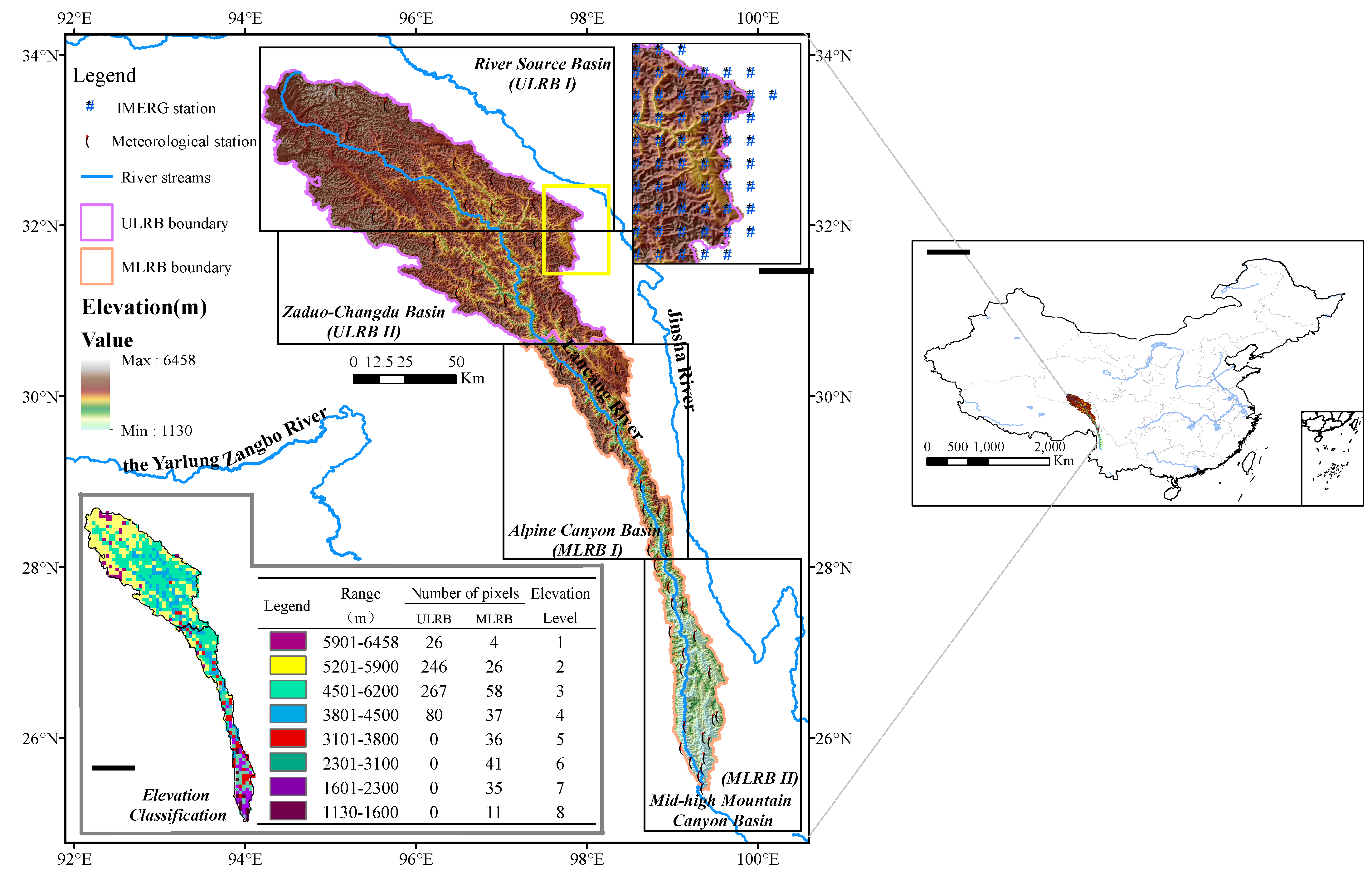
The Lancang–Mekong River Basin (LMRB) is a north–south–trending transnational river system in Central Asia that originates in the Tanggula Mountains of the central Qinghai–Tibet Plateau, flows southward through Tibet into Yunnan, leaves China in Xishuangbanna in southern Yunnan, and finally reaches the South China Sea after flowing through several other countries. The LRB has complex topography, perennial monsoon influence, and covers a wide range of latitude and elevation; it can be divided by topographic and climatic characteristics into upper, middle, and lower subbasins from north to south [49,50]. We focused on the upper (ULRB) and middle (MLRB) basins, which together cover 90,100 km2 (94.16–99.63° E and 25.38–33.83° N) (Figure 1). The ULRB (Piedmont of Qinghai–Tibet Plateau–Changdu, 31–32.9° N) is a high–elevation (average > 4500 m) Alpine Climate Region within the Qinghai–Tibet Plateau, with steep snowy peaks as well as relatively gentle terrain and broad river valleys. River flow is generally gentle and downward erosion is weak; the basin can be divided into River Source Basin (ULRB I) and the Zaduo–Changdu Basin (ULRB II). Precipitation in the ULRB is slightly higher in summer (~100 mm). In winter, cold air from westerly winds and strong radiation cooling effect in high–elevation areas can result in extreme minimum temperatures below –30 °C. The MLRB (Changdu–Guoguo Bridge, 25.4–31° N) has a wide elevation range (average 2520 m) with a great difference in elevation (more than 3000 m) and can be divided into an Alpine Canyon Basin (MLRB I) and a Mid–high Mountain Canyon Basin (MLRB II). The area spans a climatic transition from frigid to temperate to subtropical. Rainstorms are common, with an annual precipitation of 1000–1500 mm, mostly occurring from May to October. Vertical variations in air temperature and precipitation are distinct due to the topographic variance. Overall, the study area’s complex climatic (ranging from frigid alpine to subtropical) and topographic (ranging from plateaus to alpine canyons) conditions, driven by monsoons and elevation, increased the heterogeneity of precipitation in horizontal and vertical space, respectively. According to previous research, we defined November–April as the dry seasons and May–October as the wet seasons according to the precipitation in Upper and Middle Lancang River Basin (UMLRB).
2.2. Data
2.2.1. Rain Gauge Data
After data screening, we acquired 44 rain gauge precipitation observations from CMA meteorological stations (https://data.cma.cn accessed on 16 June 2021) and Yunnan Meteorological Service within the study area to evaluate the IMERG data. Each meteorological station has undergone a quality check by the National Meteorological Information Center to eliminate errors and inconsistent assessments, including examining extreme values and an internal consistency check, and removal of outliers [21]. These stations are more densely distributed in the river valley of MLRB II but all of them do not feature regular observation, especially at high–elevation mountainous regions in ULRB I. The rain gauge data is at hourly scale from January 2015 to December 2017 (Chinese Standard Time, UTC8). Other time–scale precipitation data are obtained from these data.
2.2.2. Satellite Data
We used three SPEs (IMERG E (near real–time “early” product), IMERG L (near real–time “late” product) and post–IMERG F (real–time “final” product)) in GPM Version 6 (0.1° × 0.1° and 3–h interval) (Table 1). We downloaded precipitation data from 1 January 2015 to 31 December 2017, and adjusted times to UTC 8 (see https://disc.gsfc.nasa.gov/datasets?keywords=GPM&page=1 accessed on 16 June 2021).
2.3. Methodology
2.3.1. Performance Representation
We used three metrics to evaluate IMERG spatial performance.
Amplitude Consistency
Amplitude consistency indicated that the degree to which rain gauge data and IMERG data were consistent in terms of precipitation variation. Higher values indicated more consistency (i.e., better IMERG performance). In this paper, we used four statistical indices to comprehensively quantify the amplitude consistency: (1) Correlation coefficient (CC): the correlation between IMERG and rain gauge data (1 = perfect score). (2) Root mean square error (RMSE): the degree of discretization between IMERG and rain gauge data, reflecting the overall error level and accuracy of IMERG. (3) Standard deviation (SD): the discretization of IMERG. The larger the SD, the greater the discretization. Both RMSE and SD were standardized, with perfect scores for the new root mean square error (SRMSE) and standard deviation (SSD) being 0 and 1, respectively. (4) Percentage of bias (PBias): the degree of deviation between IMERG and rain gauge data, in which positive (negative) values indicated that IMERG overestimated (underestimated) precipitation (0 = perfect score). Overall, the closer the value of the four statistical indices was to the perfect score, the better the amplitude consistency was.2.3.1.2 Occurrence consistency.
Occurrence consistency indicated that the degree to which IMERG and rain gauge data were consistent with the probability of precipitation events. Higher values indicated an increased probability of IMERG correctly detecting precipitation (i.e., better performance). In this paper, four statistical indices were used to comprehensively quantify the occurrence consistency: (1) Detection probability (POD): the ratio of the total number of precipitation events correctly detected to the total number of observed precipitation events, measuring the ability of IMERG to accurately predict precipitation events (1 = perfect score). (2) False alarm ratio (FAR): the ratio of the total number of precipitation events detected incorrectly to the total number of precipitation events detected, quantifying the possibility of false events detected by IMERG (0 = perfect score). (3) Frequency deviation (FB): the relative deviation of precipitation events recorded by IMERG and rain gauge data. FB > 0 (<0) indicated that the dataset overestimated (underestimated) the number of precipitation events (0 = perfect score). (4) Critical success index (CSI): a function of POD and FAR, indicating the overall ratio of precipitation events correctly detected by IMERG (1 = perfect score). All in all, the closer the value of the four statistical indices was to the perfect score, the better the occurrence consistency was.2.3.1.3 Elevation dependence.
Elevation dependence referred to the sensitivity of IMERG performance (or precipitation) to elevation. Positive values indicated increased performance (or precipitation) with increasing elevation and negative values indicated the opposite. The more significant the elevation–dependence, the greater the degree of performance enhancement or weakening (precipitation increase or decrease) with increasing elevation. In this paper, elevation dependence can be divided into the following three types: elevation dependence of precipitation, elevation dependence of amplitude consistency and elevation dependence of occurrence consistency.
Assuming that the precipitation is greater than the 0.1 mm/day, precipitation will occur. See Table 4 for details.
2.3.2. Linear Regression (LR) and Local Weighted Regression (LOWERG)
We used linear regression (LR) and local weighted regression (LOWERG) to analyze the relationship between precipitation and elevation in the UMLRB. The specific steps of the LR model are as follow: (1) fitting to minimize and (2) outputting where is the nonnegative weight value. When data with high periodicity and volatility are fitted using LR, a large deviation will result. LOWESS deals with this problem by fitting a line in line with the overall trend in two steps: (1) fitting to minimize and (2) outputting . If is large for a particular , should be chosen to make as small as possible. If is very small, the error term of is ignored in the fitting process. is calculated as:
When the sample point is close to the prediction point , the weight is large. .
When the sample point is far from the prediction point , the weight is small. .
is the attenuation factor, i.e., the rate of weight attenuation. The smaller the value of , the faster the weight attenuation.
2.3.3. Regional and Elevation Level Division
As mentioned in Section 2.1, ULRB and MLRB were classified as Alpine Climate Region and Climate Transition Zone respectively according to the climate. Besides, they were classified into Plateau Area and Alpine Canyon Area respectively according to the topography (Table 5).
We resampled DEM (30 m) into 0.1° by the Cubic Convolution Interpolation (CCI). CCI calculated the weighted average of DEM by using the centers of the 16 nearest input units and their values, which ensured the authenticity of the data to the greatest extent. Each pixel corresponded to one precipitation station. According to the DEM (lower left corner of Figure 1), the terrain elevation was divided into eight levels. The ULRB had 619 pixels with an elevation range of 3801–6458 m, covering four levels. The MLRB had 248 pixels, with mountains and valleys accounting for approximately half of the total pixels.
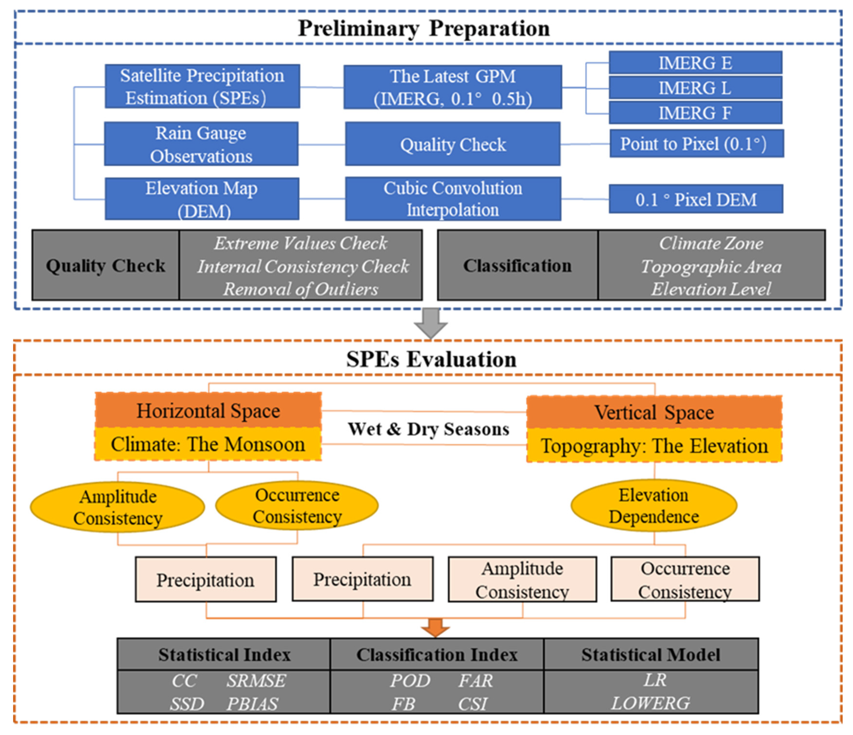
2.3.4. Analytical Procedure
Based on the two driving factors of climate and elevation, we assessed the spatial performance of IMERG in terms of (1) horizontal space (climate), which considered multi–year average precipitation, amplitude consistency, and occurrence consistency of precipitation in dry and wet seasons in the Alpine Climate Region and Climate Transition Zones and (2) vertical space (topography), which considered the elevation dependence of precipitation, amplitude, and occurrence in dry and wet seasons in the Plateau Area (ULRB) and Alpine Canyon Area (MLRB) (Figure 2).
3. Results
3.1. Multi–Year Average Precipitation and Precipitation in Dry/Wet Seasons in UMLRB
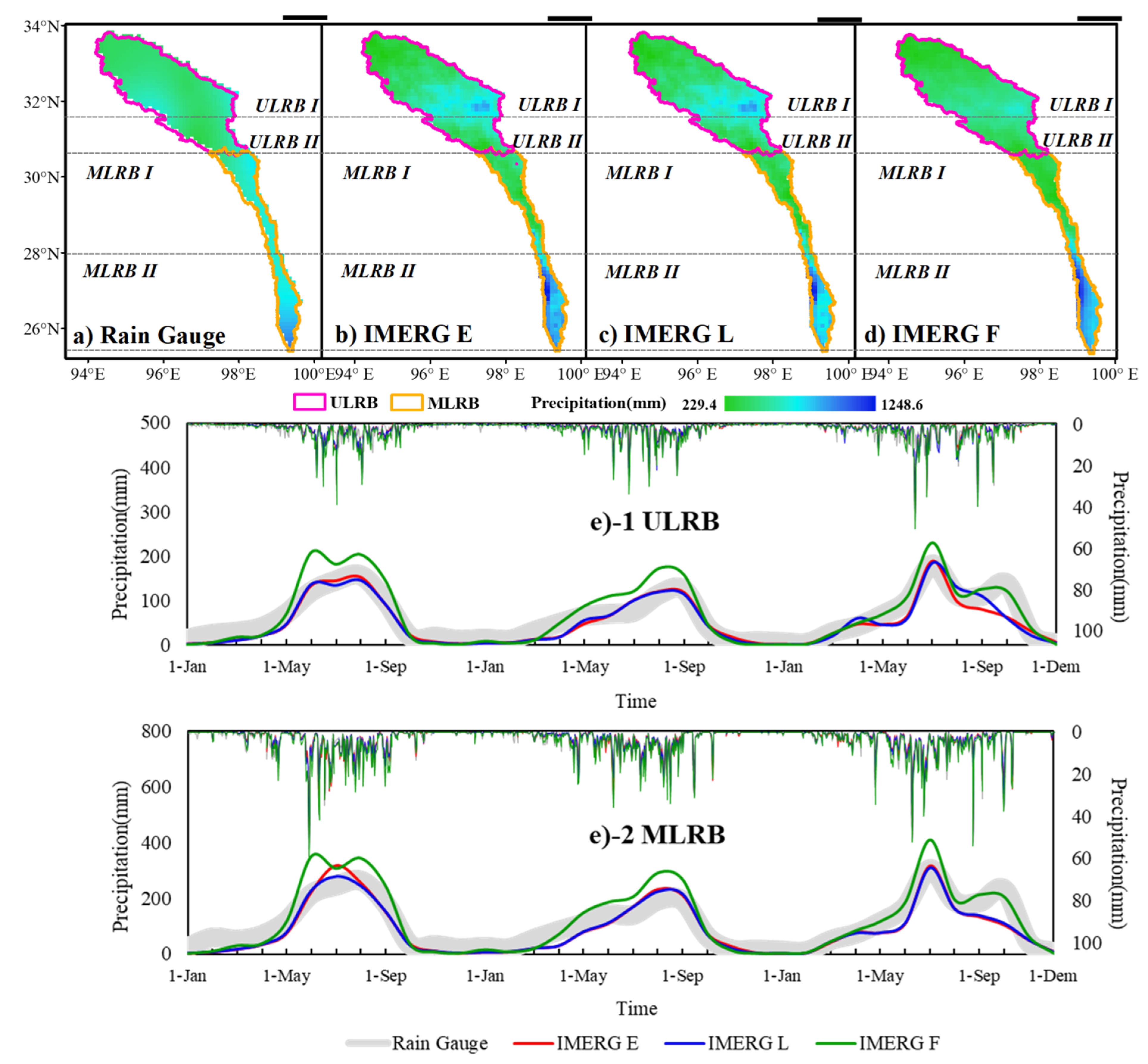
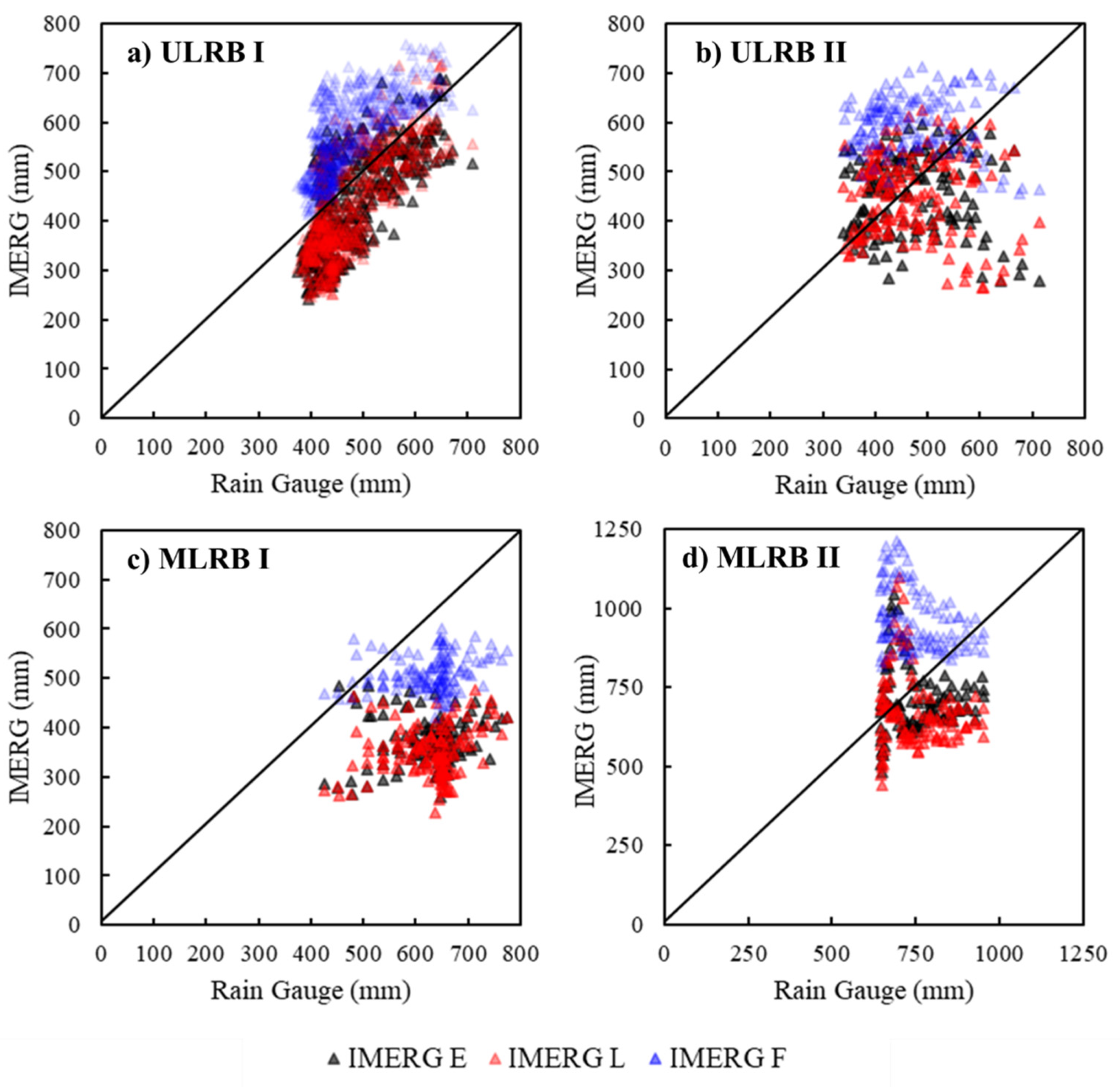
IMERG accurately captured the distribution of precipitation in the dry and wet seasons in different horizontal spaces within UMLRB. The spatial heterogeneity of multi–year average precipitation was significant, and the regularity of the precipitation distribution was strong. Precipitation increased gradually from the foothills of the northern Qinghai–Tibet Plateau to the middle reaches, with an annual average precipitation range of 229–1249 mm (Figure 3). Combined with Figure 3a–d and Figure A1 from Appendix A, it is interesting that almost all IMERG versions overestimated precipitation in ULRB I at high elevations, largely underestimated it in MLRB I, and slightly underestimated it in MLRB II. Besides, in ULRB II, odds of overestimating or underestimating were roughly the same in IMERG E and IMERG L while IMERG F tended to overestimate precipitation (Figure A1). Figure 3e showed that monthly precipitation in ULRB was higher from May to October (100–200 mm) and the difference between dry and wet seasons was ambiguous. However, precipitation in MLRB was abundant and concentrated in summer. In comparison, the transition period between spring and autumn was shorter, so there was a clear distinction between the dry and wet seasons.
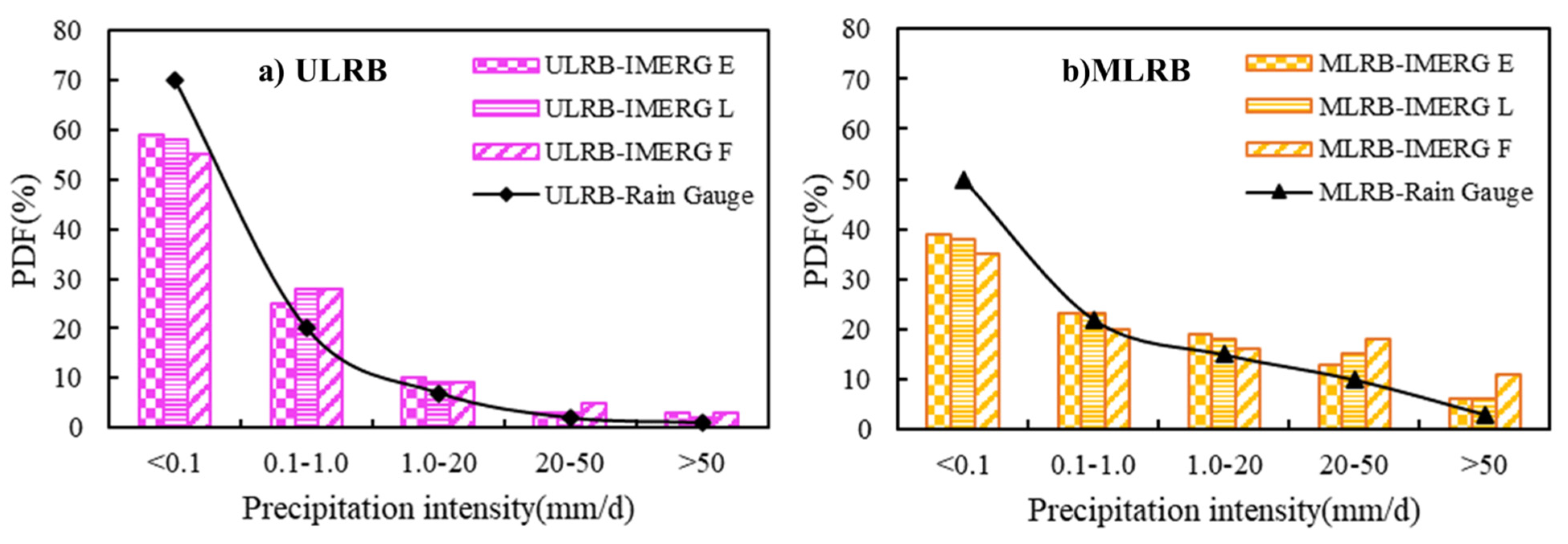
The probability density distribution of precipitation differed between ULRB and MLRB, and the probability of IMERG detecting different precipitation intensities also differed from the rain gauge. As shown in Figure 4, ~70% and ~50% of ULRB and MLRB had no precipitation probability events, respectively. In comparison, IMERG underestimated this by ~10%. In other words, IMERG tended to overestimate precipitation events. For light rain (0.1–1.0 mm/d), the precipitation probability of ULRB was roughly the same as that of MLRB (~ 23%), and IMERG slightly overestimated this in the ULRB. For moderate rain (1.0–20 mm/d), heavy rain (20–50 mm/d), and extreme precipitation (>50 mm/d), the precipitation probability of MLRB was ~10%, ~5%, and ~5% higher than that of ULRB, respectively. These results show that IMERG accurately detected differences in precipitation in the two climate zones under the influence of monsoons.
3.2. Influence of Monsoons on IMERG Horizontal Spatial Performance in UMLRB
3.2.1. Amplitude Consistency of Precipitation in Dry/Wet Seasons
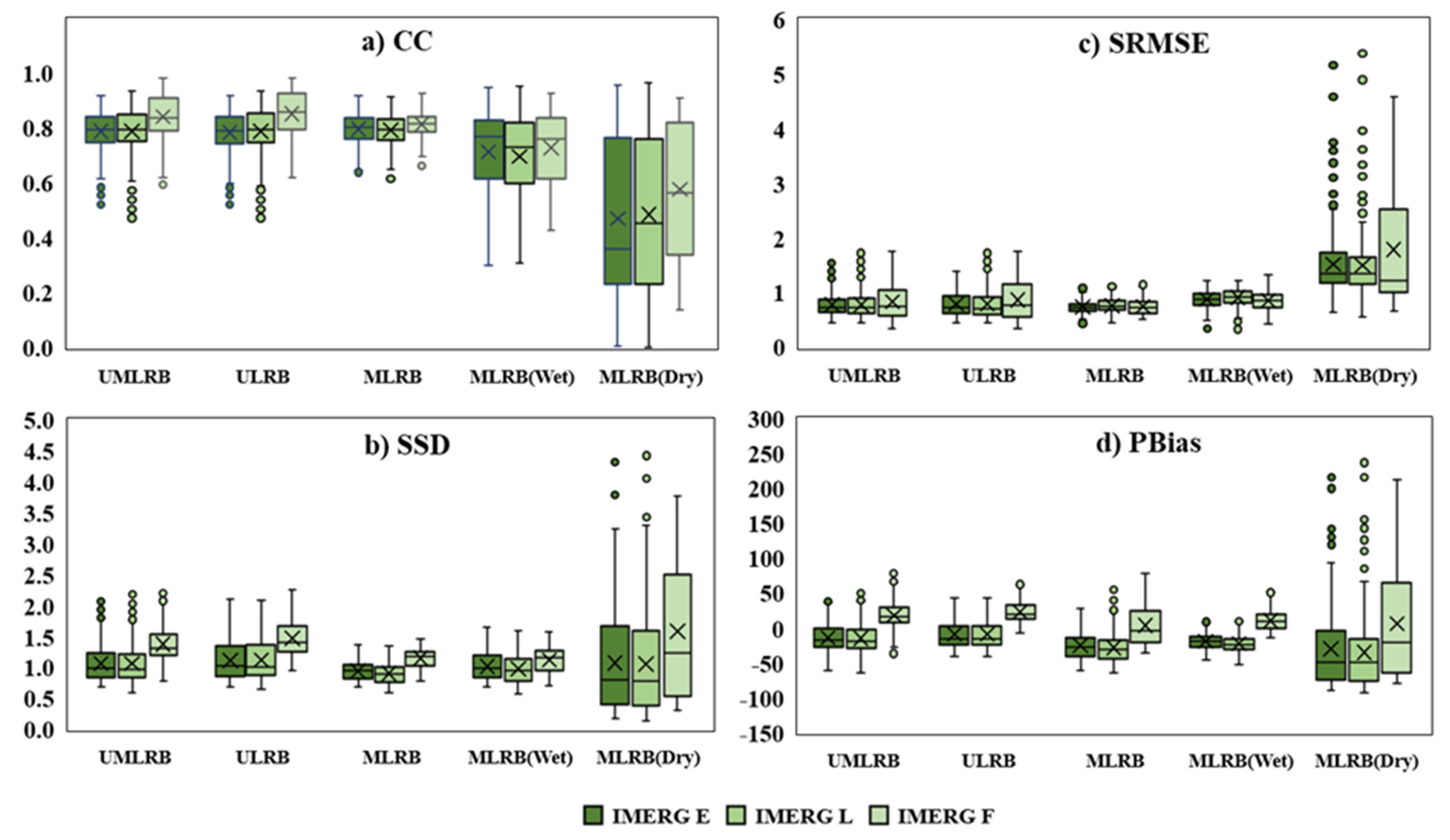
Daily precipitation from IMERG and rain gauge observations was used to evaluate the amplitude consistency of IMERG precipitation in dry and wet seasons in a horizontal space of 0.1° (Figure 5 and Figure 6). Overall, IMERG performed well in UMLRB, ULRB, and MLRB with higher CC values (mean > 0.8), more balanced SRMSE values (mean ~0.8), SSD values, and more reasonable PBias values (mean between –10 and 30). Although all the three SPEs’ performances were relatively weak in MLRB(Dry), IMERG F still performed best. Except for MLRB (Dry), IMERG F showed the outstanding performance with an average CC of ~0.8 and maximum of >0.9 (Figure 5a), but also had a high degree of discretization (Figure 5c) and tended to overestimate precipitation (Figure 5d).
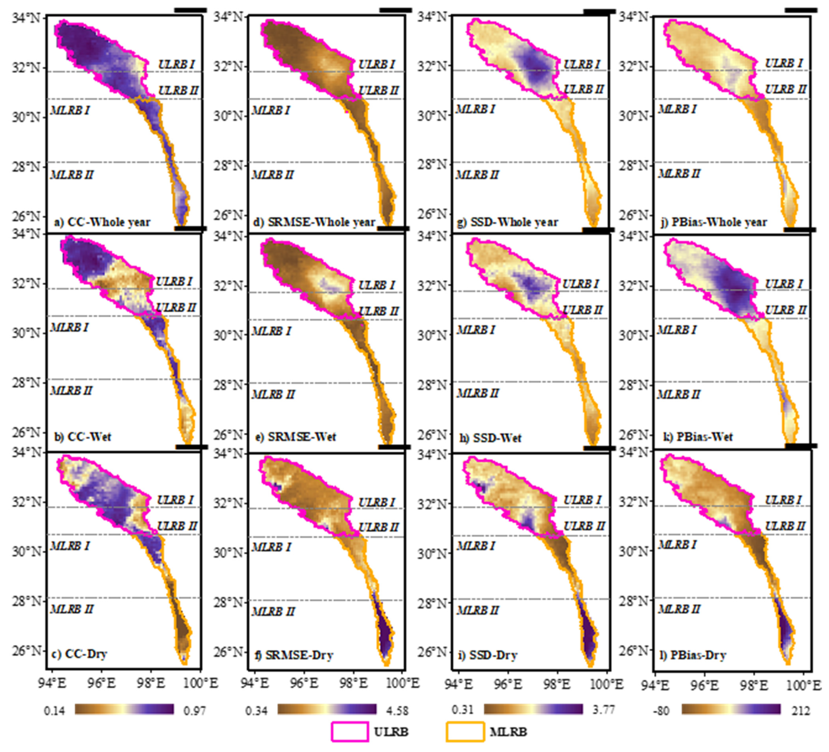
Previous studies have shown differences in IMERG performance between dry and wet seasons [26]. Figure 6 shows a comparative map of CC, SRMSE, SSD, and PBias between IMERG and rain gauge observations in the two climatic regions, i.e., the consistent spatial distribution of precipitation in the dry and wet seasons (results expressed by the means of three IMERG types). During the dry season, IMERG performed well in the Alpine Climate region overall, although CC was lower (<0.5) in the high–elevation area of ULRB I and precipitation was underestimated in most of ULRB II (PBias < 0). However, its performance in the Climate Transition Zone (MLRB) was very poor; for example, the correlation between IMERG and rain gauge observations was very low (minimum of CC < 0.2). The dispersion degree of IMERG and rain gauge observations was very high (mean SRMSE > 1.5), and the highest SRMSE value in MLRB II was >4. The IMERG data were discrete (mean SSD > 1.2), and the highest SSD value for MLRB II was >3. There was obvious underestimation and overestimation in most of MLRB I and a small portion of MLRB II, respectively. In wet seasons, IMERG performed well in ULRB I, but not ULRB II (CC < 0.5, local maximum of PBias > 3). In addition, it tended to overestimate precipitation in ULRB II (local maximum of SRMSE > 200). The overall performance of MLRB was good, except for MLRB II, which had a poor correlation (CC ~0.4).
3.2.2. Occurrence Consistency of Precipitation in Dry/Wet Seasons
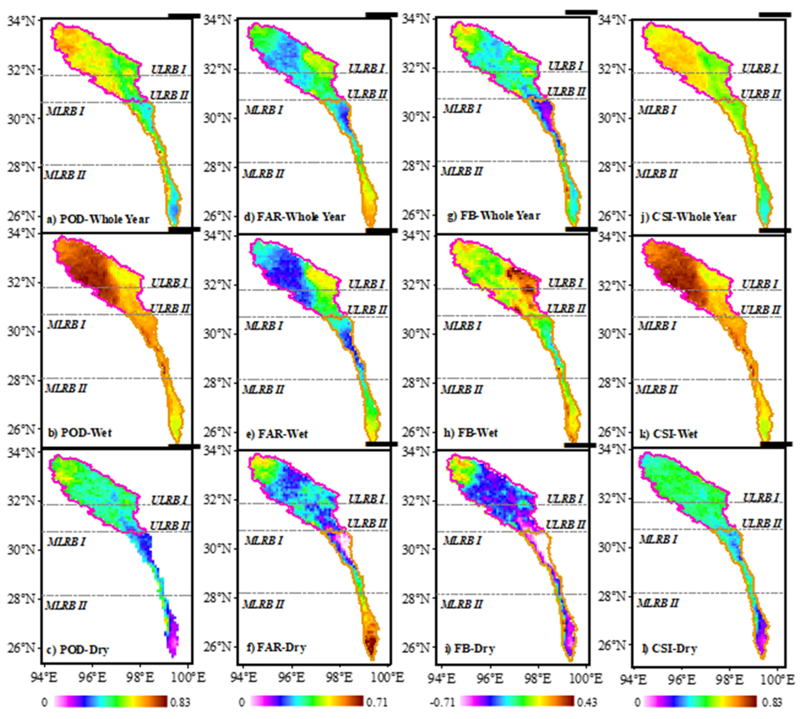
To analyze the consistency of precipitation in dry and wet seasons by horizontal space, we drew a spatial comparison map of POD, FAR, FB, and CSI between IMERG and rain gauge observations (Figure 7). The Alpine Climate Region (ULRB) showed good performance in wet seasons as a whole, except that some parts of ULRB II tended to experience misdetections and overestimations (FAR was ~0.7 and maximum FB was 0.43). In contrast, in the dry season, the overall performance of IMERG in ULRB was poor (the value of POD in a large area was only ~0.4). ULRB I tended to experience misdetection and underestimation of the probability of precipitation events (FAR > 0.3, FB fluctuated around –0.3). For the Climate Transition Zone (MLRB), IMERG performed well in the wet season as a whole, except for MLRB II, which had a higher probability of mistaken detection (FAR > 0.35). In contrast, during the dry season, the overall IMERG performance was poor, and the probability of precipitation events was underestimated over a large area of the basin (minimum FB of –0.71). In addition, there was a lower probability of correctly detecting precipitation events in MLRB II.
3.3. Influence of Topography on the Vertical Spatial Performance of IMERG in UMLRB
3.3.1. Elevation Dependence of Precipitation in Dry/Wet Seasons
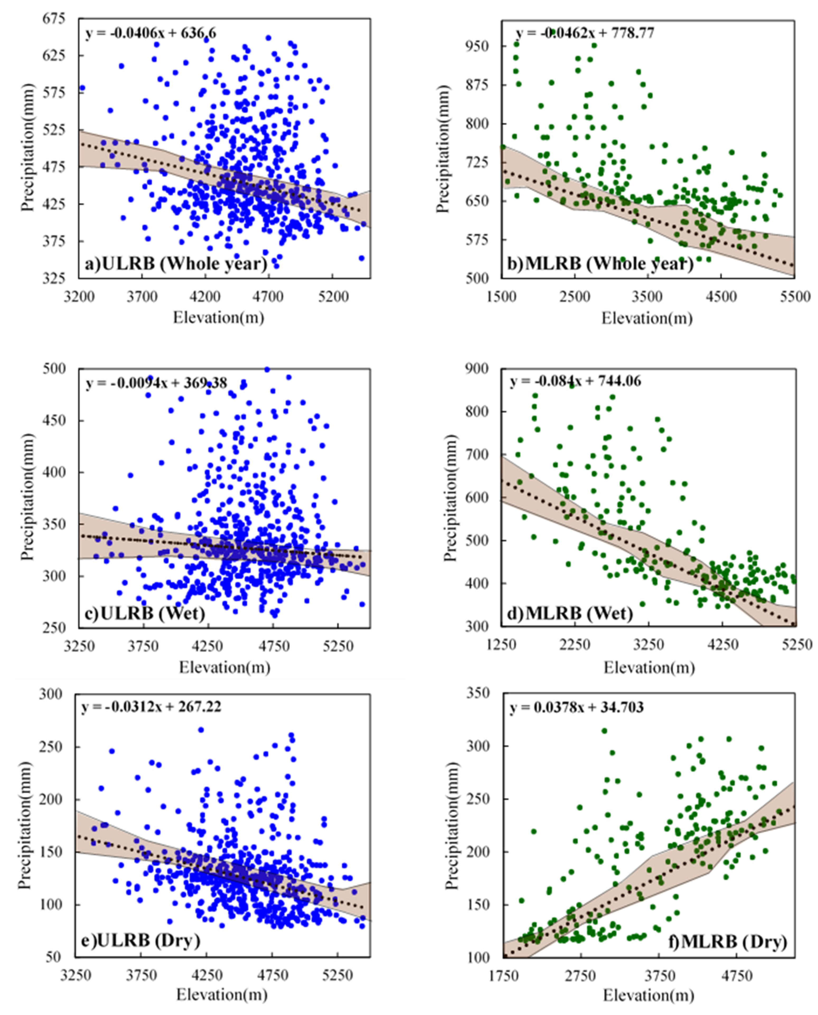
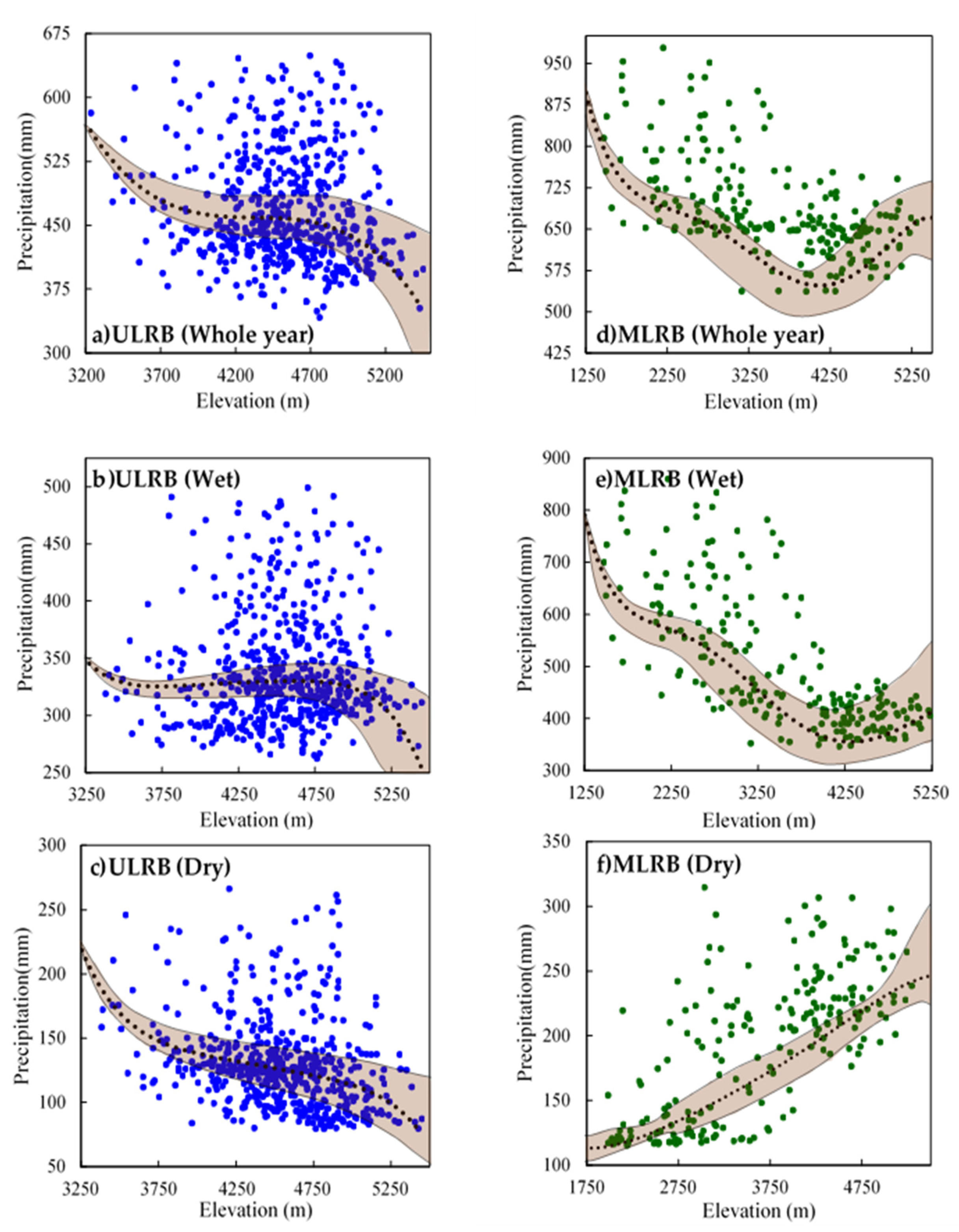
To analyze the influence of complex topography on precipitation as a whole, we developed a scatter map of precipitation and elevation over the whole year, dry season, and wet season from 2015–2017 based on LR (Figure 8). Precipitation showed a similar trend in the Plateau Area and Alpine Canyon Area throughout the year, decreasing with increasing elevation (Figure 8a,d). During the wet season, precipitation in the Alpine Canyon Area was 1.5 to 2 times higher than that in the Plateau Area (Figure 8b,e). With increasing elevation, precipitation in the Plateau Area decreased slightly (maintained at 300–350 mm), while precipitation in the alpine canyon decreased significantly (>300 mm). Slight precipitation was concentrated in the high mountains, while strong precipitation was denser in the valleys. In the dry season (Figure 8c,f), precipitation in UMLRB was relatively low. Precipitation in the Plateau Area decreased with increasing elevation, whereas precipitation in the Alpine Canyon Area increased.
3.3.2. Elevation Dependence of Amplitude in Dry/Wet Seasons
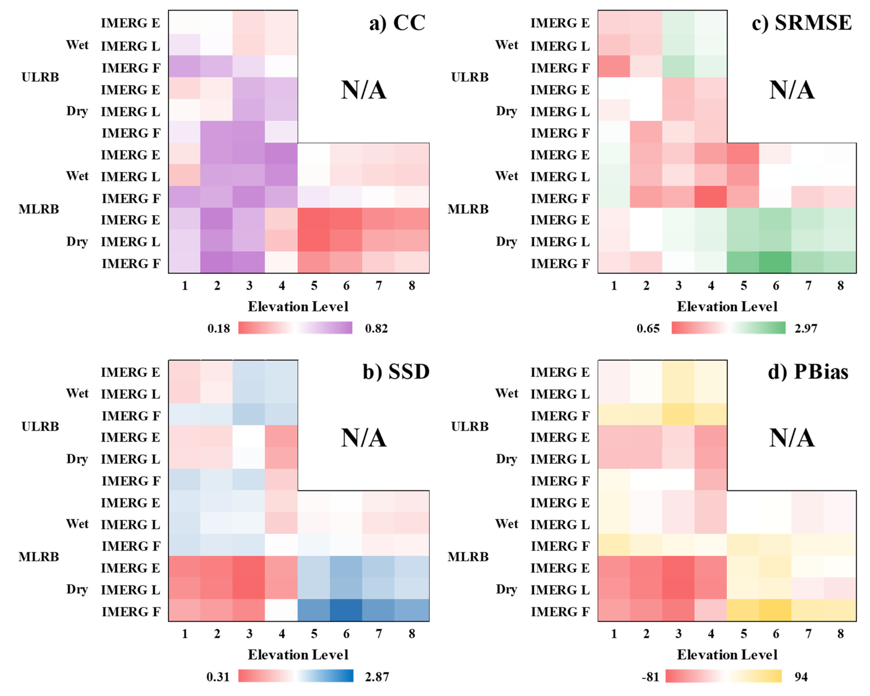
The amplitude of IMERG in the dry and wet seasons and its elevation dependence had a certain regularity at different elevation levels (Figure 9). Generally speaking, IMERG performed best in the Alpine Canyon Area in wet seasons (except for SSD > 1 at high elevations), but worst in the Alpine Canyon Area at low elevation (below 4000 m) in dry seasons (CC only ~0.2, SRMSE > 2, SSD > 2, maximum PBias of 94) (Figure 9). This suggested that the dry season limited IMERG performance to some extent, supporting the previous conclusion (Section 3.2.1) that IMERG performance differed between the dry and wet seasons.
The elevation dependence of IMERG in the Plateau Area was quite different from that in the Alpine Canyon Area, so elevation levels 1–4 were taken as an example for comparative analysis (Figure 9). In the wet season, the amplitude consistency of the dry and wet seasons in the Plateau Area was generally positively elevation–dependent. The elevation dependence of SSD and PBias was strongest, while that of CC was slightly weaker. Overall, the amplitude consistency of dry and wet seasons in the Alpine Canyon Area showed a very significant negative elevation dependence. For example, with an increase in elevation, the performance of the Plateau Area improved for SSD, while that of the Alpine Canyon Area worsened. For PBias, the Plateau Area first increased and then decreased to the optimal value (0), while the PBias of the alpine canyon region gradually increased to 90, reflecting overestimated precipitation. In the dry season, the consistency of precipitation in the dry and wet seasons in the Plateau Area generally showed negative elevation dependence. The negative elevation dependence of CC and SSD was significant. In contrast, the amplitude consistency of the dry and wet seasons in Alpine Canyon Area showed a significant positive dependence. For example, with increasing elevation, the CC of the Plateau Area decreased (0.8–0.3), while that of the Alpine Canyon Area increased (0.3–0.8).
From the perspective of the Alpine Canyon Area, the entire region (levels 1–8) had different elevation dependence in high–elevation areas (levels 1–4). CC and SRMSE in the entire region showed positive rather than significant negative dependence in the wet season. Compared with high–elevation areas, CC, SRMSE, and SSD for the whole region showed a weak positive dependence in the dry season. Interestingly, with increasing elevation, CC and SRMSE in the dry and wet seasons both improved. At the same time, CC and SRMSE in the dry season were 2–3 times and 2 times higher than those in the wet season, respectively, indicating that the positive dependence of SRMSE in dry seasons was more significant than that in wet seasons.
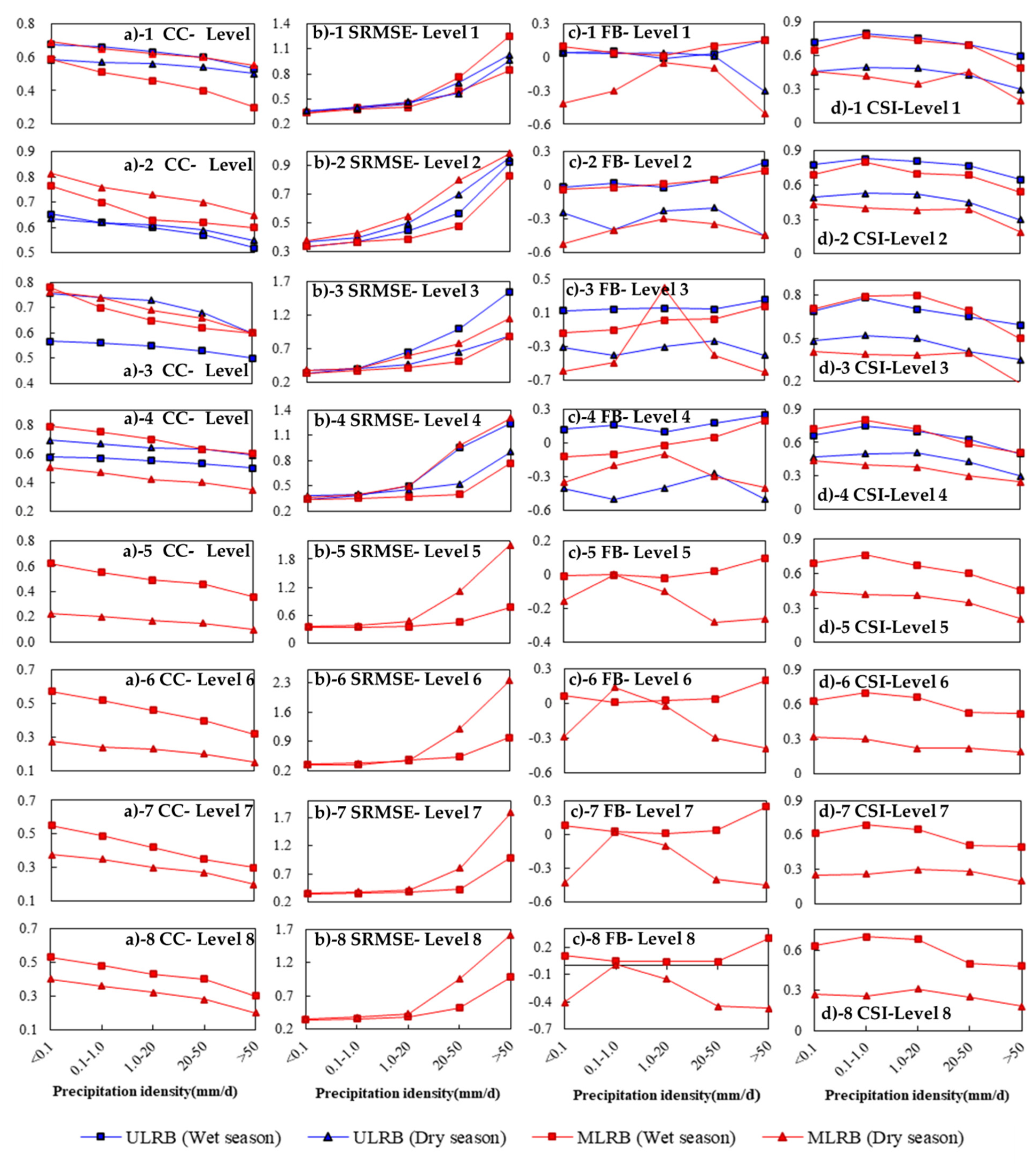
To further analyze the influence of topography on the amplitude of the dry and wet seasons, we summarized the statistical indices for different elevations under different precipitation intensities (Figure 10a,b; Figure A3a,b). The values of CC, SRMSE, SSD, and PBias for both ULRB and MLRB at all elevation levels became increasingly worse with increasing precipitation intensity in dry and wet seasons, except that the PBias of MLRB in the dry season was abnormal at high elevations (levels 1–3) (performed better in moderate rain (1.0–20 mm/d) but worse in light rain (0.1–1.0 mm/d) and extreme precipitation (>50 mm/d)). Under the same precipitation intensity, the values of CC (Figure 10(a1–a8)), SRMSE (Figure 10(b1–b8)) and SSD (Figure A3(a1–a8)) improved with increasing elevation. In MLRB, IMERG performed better (in terms of CC and SSD) in the wet season than in the dry season at low elevations (levels 4–8) (Figure 10(a4–a8), Figure A3(a4–a8)), but the opposite at high elevations (levels 1–3) (Figure 10(a1–a3), Figure A3(a1–a3)). For SRMSE in MLRB (Figure 10(b1–b8)), the performance at all elevations in the dry season was better than in the wet season, except in level 1. For PBias in MLRB (Figure A3(b1–b8)), IMERG performed better in the dry season than in the wet season at low elevations (levels 7–8), but the opposite at high elevations (levels 1–6). However, there could be a sudden and sharp decrease in amplitude consistency in the dry and wet seasons during extreme precipitation events (>50 mm/d) (Figure 10(a1,b2); Figure A3(a4,b7,b8), etc).
3.3.3. Elevation Dependence of Occurrence in Dry/Wet Seasons
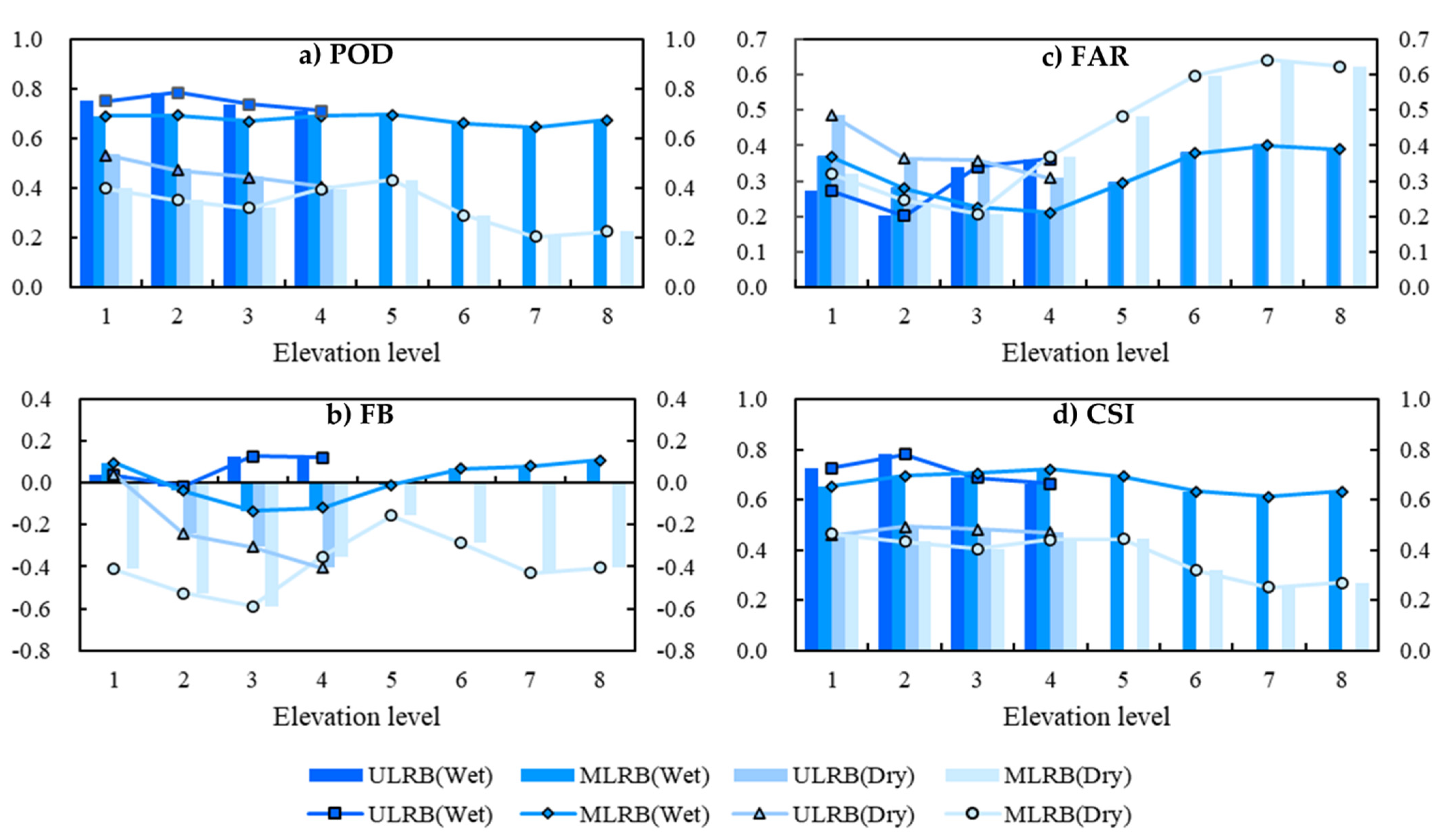
We then analyzed the performance and elevation dependence of dry and wet seasons at different elevations in the two topographic areas (Figure 11). In general, IMERG performed best in the Plateau Area during the wet season with a higher probability of correctly detecting precipitation events (mean POD ~0.8), a low probability of detecting false precipitation events (minimum FAR of 0.2), and only slight overestimation of the probability of precipitation events (FB < 0.1). However, IMERG had the worst performance in Alpine Canyon Area during the dry season (mean POD ~0.3, maximum FAR of 0.6, minimum FB of –0.6).
A comparative analysis of elevation levels 1–4 showed that generally, in the wet season, the performance of the Plateau Area was better than that of the Alpine Canyon Area. Elevation dependence in the Plateau Area was not significant, while the Alpine Canyon Area showed relatively weak negative dependence. However, during the dry season, there was a slight positive dependence in the Plateau Area (for POD and FB), but no elevation dependence in the Alpine Canyon Area, as all indices fluctuated irregularly or remained stable at all times. The elevation dependence of the Alpine Canyon Area (levels 1–8) was opposite that of the high–elevation area (levels 1–4). The four indexes in the former showed no elevation dependence in the wet season, but a certain positive elevation dependence in the dry season. CSI (from 0.3 to 0.5) had a particularly significant positive dependence.
The classification indices for precipitation in the dry and wet seasons at different elevations were analyzed (Figure 10c,d; Figure A3c,d). All four indices increasingly worsened with increasing precipitation intensity, except for FB in the MLRB, which was abnormal at high elevations (levels 1–4) in the dry season, similar to variations in PBias in MLRB with intensity (Section 3.3.2). In other words, IMERG lacked the ability to accurately detect precipitation and precipitation events in MLRB during the dry season at high elevation. IMERG had the highest probability of correctly detecting precipitation events such as light (0.1–1.0 mm/d) and moderate (1.0–20 mm/d) rain. Under the same rainfall intensity, the probability of correctly detecting precipitation events at high elevations in the dry and wet seasons in MLRB was always higher than that at low elevations (Figure 10d, Figure A3(d1–d8)). IMERG easily underestimated precipitation events in MLRB in the dry season, and the degree of underestimation at high elevations was higher. For extreme precipitation (>50 mm/d), the consistency of precipitation in dry and wet seasons could decrease suddenly and sharply as well (Figure A3(c1,c3,d1–d8); Figure 10(c1,d1–d3), etc.).
4. Discussion
4.1. Factors Affecting the Amplitude Consistency of Precipitation of IMERG in Dry and Wet Season
Amplitude consistency of precipitation by location and season ranked as: MLRB (wet) > ULRB (dry) > ULRB (wet) > MLRB (dry). The factors affecting the amplitude consistency of precipitation of IMERG in both seasons can be summarized as two points: monsoon and solid precipitation (e.g., snow).
For one thing, monsoon was one of the main sources of water vapor and some studies discussed mainly the southwest monsoon area. The precipitation gradient of the whole basin was enhanced, increasing gradually from the foothills of the Qinghai–Tibet Plateau toward the south, where precipitation sources were mainly the southwest warm &moist airflow (warm &moist in the Bay of Bengal) [50,51,52]. The Alpine Climate Region (ULRB) was little affected by the monsoon, and the distinction between dry and wet seasons was not obvious. In contrast, the Climate Transition Zone (MLRB) was greatly affected by the monsoon, with distinct dry and wet seasons. Gao et al. drew the composite field of the horizontal wind of the LRB in the wet season after 2002 and found that the northerly wind anomaly in the lower troposphere in the LRB hindered the northward movement of the southwest monsoon [50]. At the same time, there were radiation anomalies in the upper troposphere, which inhibited precipitation [50]. In this paper, it was considered that the IMERG’s performance was affected by abnormal wind field and radiation [50], so it was difficult to detect precipitation accurately, which led to the difference of precipitation amplitude between IMERG and Rain Gauge.
For another, IMERG did not perform well in winter or dry season because of the presence of snow although IMERG’s ability to retrieve solid precipitation in mountainous areas [19,27,36,38,51,53,54] was improved which can be attributed to the following reasons: 1) GPM IMERG was built on previous algorithms from PERSIANN CCS, TMPA, and CMORPH [24]; 2) the sensitivity of the dual–frequency precipitation radar (DPR) and the high–frequency channels on the GPM microware imager (GMI) were increased [16]. In other words, it can be said that the ability of IMERG to retrieve solid precipitation was improved but still limited. Many studies confirmed that the performance of SPEs in some areas (e.g., Tibetan Plateau, Wei River, Singapore, the Southern Slopes of the Pyrenees etc.) [19,24,27,36] varied with seasons and most errors were concentrated in dry seasons with snow. Our study area was located in the high–elevation area of the eastern hinterland of the Tibet Plateau where elevation was mostly above the snow line (5000 meters) with poor water vapor condition [55] and therefore it was easy to explain why IMERG tended to underestimate precipitation during the dry season in ULRB II and MLRB I.
4.2. Factors Affecting the Occurrence Consistency of Precipitation of IMERG in Dry and Wet Season
Occurrence consistency of precipitation by location and season ranked as: MLRB (wet) > ULRB (wet) > ULRB (dry) > MLRB (dry), which we believed that aerosol was the most important influencing factor. Previous studies have shown that the effect of aerosol on precipitation can be traced back to the formation, development, and decay of clouds [56,57,58,59], and its concentration had great temporal–spatial variability and seasonal heterogeneity [56], which was one of the main factors affecting climate change and atmospheric air quality. The inhibitory effect of aerosols on mild precipitation has also been reported in different parts of the world [60]. For one thing, aerosols could cool the surface and heat the nearby atmosphere by absorbing and scattering solar radiation to make the lower atmosphere more stable and precipitation suppressed to a greater extent. For another, aerosol as cloud nodule (CCN) and ice core (IN) can initiate the cloud with more but smaller cloud droplets and narrower size distribution [58,61,62], which affected the subsequent cloud microphysical processes and changed the thermodynamic and dynamic conditions and thus affected precipitation [58,63,64,65]. In short, the increase in aerosol concentration changed the size of the cloud droplets, so that the precipitation stopped or delayed.
UMLRB, originated in the Tanggula Mountains of the central TP [66,67], was representative of typical clean atmospheric conditions with low aerosol concentration [66,67]. What’s more, aerosols were removed to a large extent by widespread rainfall prevailing caused by Indian summer monsoon, which reduced its concentration over the UMLRB and its surrounding area [56]. Nevertheless, it was undeniable that the concentration of pollutants increases with the development of economy, so that the aerosol concentration of UMLRB and its surrounding areas is still rising. Dust (from Taklimakan Desert) [68] and anthropogenic pollutants [69] were the main aerosol type in the main body of UMLRB. Among them, the dust aerosols were stable mostly observed in the high–elevation areas (4–6 km) while anthropogenic pollutants tended to movable [67]. The anthropogenic pollutants could be elevated to the troposphere over the UMLRB and take part in the radiation effects and chemical reactions in the layer of troposphere [69]. In the end, the thermal structure of atmosphere and radiative budget were changed and then the precipitation was affected to some extent. To sum up, that was why ULRB I overestimated precipitation events in the wet season (maximum FB of 0.43).
4.3. Factors Affecting the Elevation Dependence of IMERG in Dry and Wet Season
Elevation dependence can be divided into elevation dependence of amplitude and elevation dependence of occurrence in dry and wet season. Using the results in Section 3.3.2 and Section 3.3.3, we had the following discussion. For elevation dependence of precipitation amplitude in both seasons, the order of significance in high–elevation areas (>4000 m) was MLRB (wet) > MLRB (dry) > ULRB (dry) ≈ ULRB (wet) while that for the whole UMLRB was MLRB (dry) > ULRB (dry) ≈ ULRB (wet) > MLRB (wet). For the elevation dependence on precipitation occurrence in both seasons, that of the Alpine Canyon Area (MLRB) in the wet season was the most significant in high–elevation areas (>4000 m), with the overall order of significance being MLRB (wet) > ULRB (wet) ≈ ULRB (dry) > MLRB (dry) and that for the whole UMLRB being MLRB (dry) > ULRB (wet) ≈ ULRB (dry) > MLRB (wet). Elevation dependence was closely related to the spatial performance of IMERG in both seasons. The elevation–dependence ranking of dry and wet seasons in Section 3.3.2 and Section 3.3.3 could verify the results given in Section 3.2.1 and Section 3.3.2 by demonstrating that the more significant the elevation dependence, the worse the IMERG performance. Similarly, the elevation dependence of IMERG precipitation amplitude in both seasons was very high in the Alpine Canyon Area (dry season), confirming that the consistency of amplitude and occurrence was the lowest there.
The factors affecting the elevation dependence of IMERG in both seasons can be summarized as two points: topography and wind–induced errors.
On the one hand, precipitation was controlled by complex topography, which made the movement of water vapor molecules change with the change of wind direction, thus affecting precipitation [43]. A sudden change in elevation may hinder the movement of the air mass (topographic rain) [70], produced a large amount of precipitation on the windward slope, or formed a microclimate on the leeward slope (the foehn effect). This complex terrain reduced the reflection sensitivity of sensors of IMERG and seriously affected the performance of them [24]. Many studies have come to the same conclusion in MLRB. Li et al. showed that the valley in the MLRB was located on the back of the windward slope with lower topography and less precipitation, which led to the foehn effect and the formation of dry and hot valleys in these areas [71]. Lin et al. showed the valleys in MLRB had less precipitation because the direction of the water vapor was changed by the wind and water vapor was blocked by multiple longitudinal mountains [55].
On the other hand, some studies confirmed that although the precipitation of rain gauge was checked to eliminate the heterogeneity and missing values, the quality of precipitation records in the high elevation (> 3000 m) was still influenced by wind–induced errors [72,73,74], which limited the applicability of IMERG in the high–elevation areas of ULRB I. Specifically, rain gauge tended to underestimate precipitation of high–elevation areas due to wind–induced errors, which may cause a slight positive deviation to the IMERG. This problem was consistent with the results of earlier studies on IMERG in high–elevation areas of Pakistan [16,75].
4.4. Effect of Altitude on Precipitation in UMLRB
Section 3.3.1 showed that precipitation throughout the year tended to decrease with increasing elevation. One explanation could be southerly or southwesterly currents carrying abundant warm and humid air from the Bay of Bengal northward to the Alpine Canyon Area, such that the north–south alpine valleys parallel to the UMLRB formed parallel flow over the three rivers (Jinsha River, Lancang River and Nu River) [38,48]. Water vapor inflow would thus become narrower and velocity would increase, leading to an increase in water vapor flux per unit area and thus precipitation at low elevations. However, the air currents would weaken gradually with elevation, making precipitation low at high elevations.
As elevation rose, precipitation detection became limited due to the influence of complex topography, potentially leading to under– or over–simulation by LR, so LOWERG was used for further comparison and discussion. Figure A2 from Appendix A showed the relationship between rain gauge precipitation and elevation based on LOWERG. Although the results of the two models (LR and LOWERG) were similar, precipitation and elevation had nonlinear relationships with certain fluctuations. For example, for the whole year (Figure A2a,d), precipitation in the Plateau Area decreased with increasing elevation, but this occurred slowly at first and then quickened; 400–500 mm was the most common precipitation range. Precipitation in the Alpine Canyon Area was lowest at ~4000 m above sea level, then began to increase again, and reaching ~650 mm at higher elevation. The influence of LOWERG on the relationship between precipitation and elevation in the Alpine Canyon Area was very significant in wet seasons (Figure A2b,e), while that in dry seasons (Figure A2c,f) was not obvious because of a slight nonlinear relationship in the Plateau Area. Overall, LOWERG could compensate for limitations caused by complex terrain and express precipitation trends in high–elevation areas.
4.5. Limitations
We focused assessed only the effects of climate and topography on IMERG performance, but future research should consider the impact of human activities (such as land use changes, landscape pattern changes and so on). In addition, the complex topographical conditions in the study area may introduce inevitable errors in precipitation data based on insufficient station density and spatial distribution. Satellite interpolation algorithms could be improved to help manage this, and infrared and microwave methods could be combined to better estimate precipitation in future. The ability of IMERG to capture different precipitation types under different climatic and topographic conditions needs to be further explored to reduce uncertainty in its precipitation estimations.
5. Conclusions
In this study, we divided the UMLRB into climatic and topographic zones by relevant features to assess the performance of GPM (three versions of IMERG) in this region from three aspects (amplitude consistency of precipitation, occurrence consistency of precipitation and elevation dependence); this is the first study to evaluate the spatial performance of IMERG under complex climatic and topographic conditions. We hope that our results can help compensate for the sparse distribution of observation stations in this region and provide a reference for IMERG hydroclimatic research, water–resource planning, and precipitation retrieval algorithm improvement under complex climate and terrain conditions while providing useful context for similar research in other mountainous areas. The main conclusions are as follows:
- The factors affecting the amplitude consistency of precipitation of IMERG in both seasons can be summarized as two points: monsoon and solid precipitation (e.g., snow). The climate difference brought spatial heterogeneity to the precipitation in dry and wet seasons. The Alpine Climate Region (ULRB) was little affected by the monsoon while the Climate Transition Zone (MLRB) was greatly affected by the monsoon. IMERG performed well in dry seasons than in wet seasons in ULRB, while the MLRB was opposite. The ability for IMERG to detect precipitation accurately of wet seasons in ULRB was limited due to the abnormal wind field and radiation, which led to the difference of precipitation amplitude between IMERG and rain gauge. Although IMERG’s ability to retrieve solid precipitation areas was improved, it tended to underestimate precipitation during the dry season in ULRB II and MLRB I due to the presence of snow. IMERG E and IMERG L tended to underestimate precipitation while IMERG F often overestimated precipitation.
- Aerosol was regarded as the most important influencing factor of occurrence consistency of precipitation in UMLRB. The increase in aerosol concentration changed the size of the cloud droplets, the thermal structure of atmosphere and radiative budget, so that the precipitation was affected to some extent. UMLRB was representative of typical clean atmospheric conditions with low aerosol concentration but aerosol concentration (dust and anthropogenic pollutants) was still increasing, which led to overestimation of precipitation events in the wet season in some areas such as ULRB I.
- Topography and wind–induced errors were the main factors affecting elevation dependence of IMERG in both seasons in UMLRB. The complex topography brought the foehn effect to the leeward slope of MLRB, which reduced the reflection sensitivity of sensors of IMERG and enhanced the elevation dependence in wet seasons in MLRB. At the same time, rain gauge tended to underestimate precipitation of high–elevation areas due to wind–induced errors.
- The LOWERG model accurately simulated the nonlinear relationship between precipitation and elevation in both seasons, compensating for IMERG’s lack of sufficient precipitation detection ability in complex terrain, especially in high–elevation areas.
- Under the same precipitation intensity, the amplitude consistency and the occurrence consistency of both seasons increased with elevation, which worsened with increasing precipitation intensity regardless of elevation. In the case of extreme precipitation (>50 mm/d), the IMERG amplitude consistency in both seasons decreased sharply. IMERG had the highest probability of correctly detecting precipitation events such as light (0.1–1.0 mm/d) and moderate (1.0–20 mm/d) rain.
GPM IMERG satellite precipitation estimation accurately represented the spatial heterogeneity of complex climate and topography in terms of precipitation and elevation dependence in both dry and wet seasons, demonstrating its great potential for wide application to hydroclimatic research in areas such as the LRB in future. In particular, in regions where observation stations are unevenly distributed or insufficiently numerous, IMERG could effectively replace observed precipitation data. Our results provide a scientific reference for similar mountain areas around the world and for the further improvement of the IMERG precipitation retrieval algorithm and the expansion of data application methods.
Author Contributions
Conceptualization, C.L. and G.F.; methodology, C.L. and G.F.; software, C.L.; validation, G.F.; formal analysis, C.L.; investigation, C.L.; data curation, C.L.; writing—original draft preparation, C.L.; writing—review and editing, J.Y. and G.F.; visualization, M.Y.; supervision, J.Y. and G.F.; project administration, G.F. and X.H.; funding acquisition, G.F. and X.H. All authors have read and agreed to the published version of the manuscript.
Funding
This research was funded by National Key Research and Development Program of China (2019YFE0105200); Fundamental Research Funds for the Central Universities (2019B11014); Water Conservancy Science and Technology Program of Jiangsu (2019016).
Institutional Review Board Statement
Not applicable.
Informed Consent Statement
Not applicable.
Data Availability Statement
Not applicable.
Conflicts of Interest
The authors declare no conflict of interest.
Appendix A
Figure A1.
Relationship between rain gauging and IMERG data (IMERG E (black), IMERG L (red) and IMERG F (blue)) at average annual scale in (a) ULRB I, (b) ULRB II, (c) MLRB I and (d) MLRB II. One point represents one pixel.
Figure A1.
Relationship between rain gauging and IMERG data (IMERG E (black), IMERG L (red) and IMERG F (blue)) at average annual scale in (a) ULRB I, (b) ULRB II, (c) MLRB I and (d) MLRB II. One point represents one pixel.

Figure A2.
Relationship between rain gauge precipitation and elevation based on LOWESS for the whole year (top row), wet season (middle row), and dry season (bottom row) in the (a–c) ULRB and (d–f) MLRB. One point represents one pixel.
Figure A2.
Relationship between rain gauge precipitation and elevation based on LOWESS for the whole year (top row), wet season (middle row), and dry season (bottom row) in the (a–c) ULRB and (d–f) MLRB. One point represents one pixel.

Figure A3.
Trend chart of changes in four indices (a) SSD, (b) PBias, (c) POD, and (d) FAR by precipitation intensity for different regions and seasons by elevation levels (1–8).
Figure A3.
Trend chart of changes in four indices (a) SSD, (b) PBias, (c) POD, and (d) FAR by precipitation intensity for different regions and seasons by elevation levels (1–8).

References
- Brutsaert, W. Hydrology: An Introduction; Cambridge University Press: Cambridge, UK, 2005. [Google Scholar]
- Udo, S.; Ziese, M.; Meyer–Christoffer, A.; Finger, P.; Rustemeier, E.; Becker, A. The New Portfolio of Global Precipitation Data Products of the Global Precipitation Climatology Centre Suitable to Assess and Quantify the Global Water Cycle and Resources. Proc. Int. Assoc. Hydrol. Sci. 2016, 374, 29–34. [Google Scholar]
- Daly, C.; Slater, M.E.; Roberti, J.A.; Laseter, S.H.; Swift, L.W., Jr. High–Resolution Precipitation Mapping in a Mountainous Watershed: Ground Truth for Evaluating Uncertainty in a National Precipitation Dataset. Int. J. Climatol. 2017, 37, 124–137. [Google Scholar] [CrossRef] [Green Version]
- Sun, Q.; Miao, C.; Duan, Q.; Ashouri, H.; Sorooshian, S.; Hsu, K.-L. A Review of Global Precipitation Data Sets: Data Sources, Estimation, and Intercomparisons. Rev. Geophys. 2018, 56, 79–107. [Google Scholar] [CrossRef] [Green Version]
- Wanders, N.; Pan, M.; Wood, E.F. Correction of Real–Time Satellite Precipitation with Multi–Sensor Satellite Observations of Land Surface Variables. Remote Sens. Environ. 2015, 160, 206–221. [Google Scholar] [CrossRef]
- Chung–Chen, J.; Kot, S.C.; Tepper, M. Comparing Noaa–12 and Radiosonde Atmospheric Sounding Profiles for Mesoscale Weather Model Initialization. In Proceedings of the COSPAR Colloquia Series, Tainan, Taiwan, 14–17 December 1997; Volume 8, pp. 103–109. [Google Scholar]
- Shi, H.; Li, T.; Wei, J. Evaluation of the Gridded Cru Ts Precipitation Dataset with the Point Raingauge Records over the Three–River Headwaters Region. J. Hydrol. 2017, 548, 322–332. [Google Scholar] [CrossRef] [Green Version]
- Yuan, F.; Wang, B.; Shi, C.; Cui, W.; Zhao, C.; Liu, Y.; Ren, L.; Zhang, L.; Zhu, Y.; Chen, T.; et al. Evaluation of Hydrological Utility of Imerg Final Run V05 and Tmpa 3b42v7 Satellite Precipitation Products in the Yellow River Source Region, China. J. Hydrol. 2018, 567, 696–711. [Google Scholar] [CrossRef]
- Chappell, A.; Renzullo, L.J.; Raupach, T.H.; Haylock, M. Evaluating Geostatistical Methods of Blending Satellite and Gauge Data to Estimate near Real–Time Daily Rainfall for Australia. J. Hydrol. 2013, 493, 105–114. [Google Scholar] [CrossRef]
- Li, Z.; Yang, D.; Hong, Y. Multi–Scale Evaluation of High–Resolution Multi–Sensor Blended Global Precipitation Products over the Yangtze River. J. Hydrol. 2013, 500, 157–169. [Google Scholar] [CrossRef]
- Qin, Y.; Chen, Z.; Shen, Y.; Zhang, S.; Shi, R. Evaluation of Satellite Rainfall Estimates over the Chinese Mainland. Remote Sens. 2014, 6, 11649–11672. [Google Scholar] [CrossRef] [Green Version]
- Hou, A.; Ramesh, Y.; Kakar, K.; Neeck, S.; Azarbarzin, A.A.; Kummerow, C.D.; Kojima, M.; Oki, R.; Nakamura, K.; Iguchi, T. The Global Precipitation Measurement Mission. Bull. Am. Meteorol. Soc. 2014, 95, 701–722. [Google Scholar] [CrossRef]
- Palomino–Ángel, S.; Anaya–Acevedo, J.A.; Botero, B.A. Evaluation of 3b42v7 and Imerg Daily–Precipitation Products for a Very High–Precipitation Region in Northwestern South America. Atmos. Res. 2019, 217, 37–48. [Google Scholar] [CrossRef]
- Sharifi, E.; Steinacker, R.; Saghafian, B. Assessment of Gpm–Imerg and Other Precipitation Products against Gauge Data under Different Topographic and Climatic Conditions in Iran: Preliminary Results. Remote Sens. 2016, 8, 135. [Google Scholar] [CrossRef] [Green Version]
- Skofronick–Jackson, G.; Petersen, W.A.; Berg, W.; Kidd, C.; Stocker, E.F.; Kirschbaum, D.B.; Kakar, R.; Braun, S.A.; Huffman, G.J.; Iguchi, T.; et al. The Global Precipitation Measurement (Gpm) Mission for Science and Society. Bull. Am. Meteorol. Soc. 2017, 98, 1679–1695. [Google Scholar] [CrossRef]
- Anjum, M.N.; Ding, Y.; Shangguan, D.; Ahmad, I.; Ijaz, M.W.; Farid, H.U.; Yagoub, Y.E.; Zaman, M.; Adnan, M. Performance Evaluation of Latest Integrated Multi–Satellite Retrievals for Global Precipitation Measurement (Imerg) over the Northern Highlands of Pakistan. Atmos. Res. 2018, 205, 134–146. [Google Scholar] [CrossRef]
- Chen, F.; Li, X. Evaluation of Imerg and Trmm 3b43 Monthly Precipitation Products over Mainland China. Remote Sens. 2016, 8, 472. [Google Scholar] [CrossRef] [Green Version]
- Gebregiorgis, A.S.; Kirstetter, P.-E.; Hong, Y.E.; Gourley, J.J.; Huffman, G.J.; Petersen, W.A.; Xue, X.; Schwaller, M.R. To What Extent Is the Day 1 Gpm Imerg Satellite Precipitation Estimate Improved as Compared to Trmm Tmpa–Rt? J. Geophys. Res. Atmos. 2018, 123, 1694–1707. [Google Scholar] [CrossRef]
- Tan, M.; Duan, Z. Assessment of Gpm and Trmm Precipitation Products over Singapore. Remote Sens. 2017, 9, 720. [Google Scholar] [CrossRef] [Green Version]
- Yang, X.; Lu, Y.; Tan, M.L.; Li, X.; Wang, G.; He, R. Nine–Year Systematic Evaluation of the Gpm and Trmm Precipitation Products in the Shuaishui River Basin in East–Central China. Remote Sens. 2020, 12, 1042. [Google Scholar] [CrossRef] [Green Version]
- Wang, X.; Ding, Y.; Zhao, C.; Wang, J. Similarities and Improvements of Gpm Imerg Upon Trmm 3b42 Precipitation Product under Complex Topographic and Climatic Conditions over Hexi Region, Northeastern Tibetan Plateau. Atmos. Res. 2019, 218, 347–363. [Google Scholar] [CrossRef]
- Anjum, M.N.; Ahmad, I.; Ding, Y.; Shangguan, D.; Ijaz, M.Z.W.; Sarwar, K.; Han, H.; Yang, M. Assessment of Imerg–V06 Precipitation Product over Different Hydro–Climatic Regimes in the Tianshan Mountains, North–Western China. Remote Sens. 2019, 11, 2314. [Google Scholar] [CrossRef] [Green Version]
- Golian, S.; Moazami, S.; Kirstetter, P.; Hong, Y. Evaluating the Performance of Merged Multi–Satellite Precipitation Products over a Complex Terrain. Water Resour. Manag. 2015, 29, 4885–4901. [Google Scholar] [CrossRef]
- Liu, j.; Xia, J.; She, D.; Li, L.; Wang, Q.; Zou, L. Evaluation of Six Satellite–Based Precipitation Products and Their Ability for Capturing Characteristics of Extreme Precipitation Events over a Climate Transition Area in China. Remote Sens. 2019, 11, 1477. [Google Scholar] [CrossRef] [Green Version]
- Wang, S.; Liu, J.; Wang, J.; Qiao, X.; Zhang, J. Evaluation of Gpm Imerg V05b and Trmm 3b42v7 Precipitation Products over High Mountainous Tributaries in Lhasa with Dense Rain Gauges. Remote Sens. 2019, 11, 2080. [Google Scholar] [CrossRef] [Green Version]
- Yu, C.; Hu, D.; Liu, M.; Wang, S.; Di, Y. Spatio–Temporal Accuracy Evaluation of Three High–Resolution Satellite Precipitation Products in China Area. Atmos. Res. 2020, 241, 104952. [Google Scholar] [CrossRef]
- Wang, Y.; Xie, X.; Meng, S.; Wu, D.; Chen, Y.; Jiang, F.; Zhu, B. Magnitude Agreement, Occurrence Consistency, and Elevation Dependency of Satellite–Based Precipitation Products over the Tibetan Plateau. Remote Sens. 2020, 12, 1750. [Google Scholar] [CrossRef]
- Zhang, C.; Chen, X.; Shao, H.; Chen, S.; Liu, T.; Chen, C.; Ding, Q.; Du, H. Evaluation and Intercomparison of High–Resolution Satellite Precipitation Estimates—Gpm, Trmm, and Cmorph in the Tianshan Mountain Area. Remote Sens. 2018, 10, 1543. [Google Scholar] [CrossRef] [Green Version]
- Yang, M.; Liu, G.; Chen, T.; Chen, Y.; Xia, C. Evaluation of Gpm Imerg Precipitation Products with the Point Rain Gauge Records over Sichuan, China. Atmos. Res. 2020, 246, 105101. [Google Scholar] [CrossRef]
- Sharma, S.; Chen, Y.; Zhou, X.; Yang, K.; Li, X.; Niu, X.; Hu, X.; Khadka, N. Evaluation of Gpm–Era Satellite Precipitation Products on the Southern Slopes of the Central Himalayas against Rain Gauge Data. Remote Sens. 2020, 12, 1836. [Google Scholar] [CrossRef]
- de Sousa Afonso, J.M.; Vila, D.A.; Gan, M.A.; Quispe, D.P.; de Jesus da Costa Barreto, N.; Chinchay, J.H.H.; Palharini, R.S.A. Precipitation Diurnal Cycle Assessment of Satellite–Based Estimates over Brazil. Remote Sens. 2020, 12, 2339. [Google Scholar] [CrossRef]
- Li, Z.; Chen, M.; Gao, S.; Hong, Z.; Tang, G.; Wen, Y.; Gourley, J.J.; Hong, Y. Cross–Examination of Similarity, Difference and Deficiency of Gauge, Radar and Satellite Precipitation Measuring Uncertainties for Extreme Events Using Conventional Metrics and Multiplicative Triple Collocation. Remote Sens. 2020, 12, 1258. [Google Scholar] [CrossRef] [Green Version]
- Ma, M.; Wang, H.; Jia, P.; Tang, G.; Wang, D.; Ma, Z.; Yan, H. Application of the Gpm–Imerg Products in Flash Flood Warning: A Case Study in Yunnan, China. Remote Sens. 2020, 12, 1954. [Google Scholar] [CrossRef]
- Xiao, S.; Xia, J.; Zou, L. Evaluation of Multi–Satellite Precipitation Products and Their Ability in Capturing the Characteristics of Extreme Climate Events over the Yangtze River Basin, China. Water 2020, 12, 1179. [Google Scholar] [CrossRef] [Green Version]
- Yuan, F.; Zhang, L.; Soe, K.; Ren, L.; Zhao, C.; Zhu, Y.; Jiang, S.; Liu, Y. Applications of Trmm– and Gpm–Era Multiple–Satellite Precipitation Products for Flood Simulations at Sub–Daily Scales in a Sparsely Gauged Watershed in Myanmar. Remote Sens. 2019, 11, 140. [Google Scholar] [CrossRef] [Green Version]
- Navarro, A.; García–Ortega, E.; Merino, A.; Sánchez, J.L. Extreme Events of Precipitation over Complex Terrain Derived from Satellite Data for Climate Applications: An Evaluation of the Southern Slopes of the Pyrenees. Remote Sens. 2020, 12, 2171. [Google Scholar] [CrossRef]
- Alsumaiti, T.S.; Hussein, K.; Ghebreyesus, D.T.; Sharif, H.O. Performance of the Cmorph and Gpm Imerg Products over the United Arab Emirates. Remote Sens. 2020, 12, 1426. [Google Scholar] [CrossRef]
- He, Z.; Yang, L.; Tian, F.; Ni, G.; Hou, A.; Lu, H. Intercomparisons of Rainfall Estimates from Trmm and Gpm Multisatellite Products over the Upper Mekong River Basin. J. Hydrometeorol. 2017, 18, 413–430. [Google Scholar] [CrossRef]
- Yu, L.; Ma, L.; Li, H.; Zhang, Y.; Kong, F.; Yang, Y. Assessment of High–Resolution Satellite Rainfall Products over a Gradually Elevating Mountainous Terrain Based on a High–Density Rain Gauge Network. Int. J. Remote Sens. 2020, 41, 5620–5644. [Google Scholar] [CrossRef]
- Rojas, Y.; Minder, J.R. Assessment of Gpm Imerg Satellite Precipitation Estimation and Its Dependence on Microphysical Rain Regimes over the Mountains of South–Central Chile. Atmos. Res. 2021, 253, 105454. [Google Scholar] [CrossRef]
- Nepal, B.; Shrestha, D. Assessment of Gpm–Era Satellite Products’(Imerg and Gsmap) Ability to Detect Precipitation Extremes over Mountainous Country Nepal. Atmosphere 2021, 12, 254. [Google Scholar] [CrossRef]
- Joyce, R.J.; Janowiak, J.E.; Arkin, P.A.; Xie, P. Cmorph: A Method That Produces Global Precipitation Estimates from Passive Microwave and Infrared Data at High Spatial and Temporal Resolution. J. Hydrometeorol. 2004, 5, 487–503. [Google Scholar] [CrossRef]
- Gebremicael, T.G.; Mohamed, Y.A.; van der Zaag, P.; Gebremedhin, A.; Gebremeskel, G.; Yazew, E.; Kifle, M. Evaluation of Multiple Satellite Rainfall Products over the Rugged Topography of the Tekeze–Atbara Basin in Ethiopia. Int. J. Remote Sens. 2019, 40, 4326–4345. [Google Scholar] [CrossRef]
- Guo, H.; Chen, S.; Bao, A.; Behrangi, A.; Hong, Y.; Ndayisaba, F.; Hu, J.; Stepanian, P.M. Early Assessment of Integrated Multi–Satellite Retrievals for Global Precipitation Measurement over China. Atmos. Res. 2016, 176, 121–133. [Google Scholar] [CrossRef]
- Kim, J.-H.; Ou, M.-L.; Park, J.-D.; Morris, K.R.; Schwaller, M.R.; Wolff, D.B. Global Precipitation Measurement (Gpm) Ground Validation (Gv) Prototype in the Korean Peninsula. J. Atmos. Ocean. Technol. 2014, 31, 1902–1921. [Google Scholar] [CrossRef]
- Chen, J.; Wang, Z.; Wu, X.; Chen, X.; Lai, C.; Zeng, Z. Accuracy Evaluation of Gpm Multi–Satellite Precipitation Products in the Hydrological Application over Alpine and Gorge Regions with Sparse Rain Gauge Network. Hydrol. Res. 2019, 50, 1710–1729. [Google Scholar] [CrossRef] [Green Version]
- Wang, Z.; Chen, J.; Lai, C.; Zhong, R.; Chen, X.; Yu, H. Hydrologic Assessment of the Tmpa 3b42–V7 Product in a Typical Alpine and Gorge Region: The Lancang River Basin, China. Hydrol. Res. 2018, 49, 2002–2015. [Google Scholar] [CrossRef]
- Wang, W.; Lu, H.; Zhao, T.; Jiang, L.; Shi, J. Evaluation and Comparison of Daily Rainfall from Latest Gpm and Trmm Products over the Mekong River Basin. IEEE J. Sel. Top. Appl. Earth Obs. Remote Sens. 2017, 10, 2540–2549. [Google Scholar] [CrossRef]
- He, D. Analysis of Hydrological Characteristics in Lancang–Mekong River. Yunnan Geogr. Environ. Res. 1995, 7, 59–73. (In Chinese) [Google Scholar]
- Gao, H.; Xiao, Z.; Zhao, L. A Study on the Abrupt Change of Summer Rainfall over Lancang River Basin and the Associated Atmospheric Circulation in the Early 21st Century. Clim. Environ. Res. 2019, 24, 513–524. (In Chinese) [Google Scholar]
- Chen, C.; Chen, Q.; Duan, Z.; Zhang, J.; Mo, K. Multiscale Comparative Evaluation of the Gpm Imerg V5 and Trmm 3b42 V7 Precipitation Products from 2015 to 2017 over a Climate Transition Area of China. Remote Sens. 2018, 10, 944. [Google Scholar] [CrossRef] [Green Version]
- Xu, W.; Li, Q.; Wang, X.; Yang, S. Homogenization of Chinese Daily Surface Air Temperatures and Analysis of Trends in the Extreme Temperature Indices. J. Geophys. Res. Atmos. 2013, 118, 9708–9720. [Google Scholar] [CrossRef]
- Tang, G.; Ma, Y.; Long, D.; Zhong, L. Imerg and Tmpa Version–7 Legacy Products over Mainland China at Multiple Spatiotemporal Scales. J. Hydrol. 2016, 533, 152–167. [Google Scholar] [CrossRef]
- Legates, D.R.; Willmott, C.J. Mean Seasonal and Spatial Variability in Gauge–Corrected, Global Precipitation. Int. J. Climatol. 1990, 10, 111–127. [Google Scholar] [CrossRef]
- Lin, Y.; Duan, W.; Liu, Y. Analysis of Torrential Rain Characteristics in the Upper Reaches of Lancang River. Sci. Technol. Inf. 2015, 32, 104–109. (In Chinese) [Google Scholar]
- Liu, C.; Gao, Y.; Yi, J.; Yang, S. An Modis–Based Analysis of Spatio–Temporal Variations of Aerosol Optical Depth in Southwest of China. J. Southwest Univ. 2014, 36, 182–189. [Google Scholar]
- Zhou, Y.; Han, Y.; Wu, Y.; Wang, T. Optical Properties and Spatial Variation of Tropical Cyclone Cloud Systems from Trmm and Modis in the East Asia Region: 2010–2014. J. Geophys. Res. Atmos. 2018, 123, 9542–9558. [Google Scholar] [CrossRef]
- Rosenfeld, D.; Woodley, W.L.; Khain, A.; Cotton, W.R.; Carrió, G.; Ginis, I.; Golden, J.H. Aerosol Effects on Microstructure and Intensity of Tropical Cyclones. Bull. Am. Meteorol. Soc. 2012, 93, 987–1001. [Google Scholar] [CrossRef]
- Wang, Y.; Lee, K.-H.; Lin, Y. Distinct Effects of Anthropogenic Aerosols on Tropical Cyclones. Nat. Clim. Chang. 2014, 4, 368–373. [Google Scholar] [CrossRef]
- Dong, X.; Li, R.; Wang, Y.; Fu, Y. Potential Impacts of Sahara Dust Aerosol on Rainfall Vertical Structure over the Atlantic Ocean as Identified from Eof Analysis. J. Geophys. Res. Atmos. 2018, 123, 8850–8868. [Google Scholar] [CrossRef]
- Guo, J.; Liu, H.; Li, Z.; Rosenfeld, D. Aerosol–Induced Changes in the Vertical Structure of Precipitation: A Perspective of Trmm Precipitation Radar. Atmos. Chem. Phys. 2018, 18, 13329–13343. [Google Scholar] [CrossRef] [Green Version]
- Wang, Y.; Wan, Q.; Meng, W. Long–Term Impacts of Aerosols on Precipitation and Lightning over the Pearl River Delta Megacity Area in China. Atmos. Chem. Phys. 2011, 11, 12421–12436. [Google Scholar] [CrossRef] [Green Version]
- Squires, P. The Spatial Variation of Liquid Water and Droplet Concentration in Cumuli. Tellus 1958, 10, 372–380. [Google Scholar] [CrossRef] [Green Version]
- Twomey, S. The Influence of Pollution on the Shortwave Albedo of Clouds. J. Atmos. Sci. 1977, 34, 1149–1152. [Google Scholar] [CrossRef] [Green Version]
- Fan, J.; Rosenfeld, D.; Zhang, Y. Substantial Convection and Precipitation Enhancements by Ultrafine Aerosol Particles. Sci. Technol. Inf. 2018, 359, 411–418. [Google Scholar] [CrossRef] [Green Version]
- Xu, C.; Ma, Y.M.; You, C. The Regional Distribution Characteristics of Aerosol Optical Depth over the Tibetan Plateau. Atmos. Chem. Phys. 2015, 15, 12065–12078. [Google Scholar] [CrossRef] [Green Version]
- Liaoa, T.; Guib, K.; Liab, Y. Seasonal Distribution and Vertical Structure of Different Types of Aerosols in Southwest China Observed from Caliop. Atmos. Environ. 2021, 246, 118145. [Google Scholar] [CrossRef]
- Xu, X.; Wu, H.; Yang, X. Distribution and Transport Characteristics of Dust Aerosol over Tibetan Plateau and Taklimakan Desert in China Using Merra–2 and Calipso Data. Atmos. Environ. 2020, 237, 117670. [Google Scholar] [CrossRef]
- Huang, J.; Fu, Q.; Su, J. Taklimakan Dust Aerosol Radiative Heating Derived from Calipso Observations Using the Fu–Liou Radiation Model with Ceres Constraints. Atmos. Chem. Phys. 2009, 9, 4011–4021. [Google Scholar] [CrossRef]
- Dinku, T.; Ceccato, P.; Grover–Kopec, E.; Lemma, M.; Connor, S.J.; Ropelewski, C.F. Validation of Satellite Rainfall Products over East Africa’s Complex Topography. Int. J. Remote Sens. 2007, 28, 1503–1526. [Google Scholar] [CrossRef]
- Li, Q. Flora Analysis and Phytocommunity Studies on the Deciduous Monsoon Forest at Lower Reaches of Luozha River in Yunxian. Master’s Thesis, Chinese Academy of Sciences, Beijing, China, June 2007. [Google Scholar]
- Tahir, A.A.; Adamowski, J.; Chevallier, P. Comparative Assessment of Spatiotemporal Snow Cover Changes and Hydrological Behavior of the Gilgit, Astore and Hunza River Basins (Hindukush–Karakoram–Himalaya Region, Pakistan). Meteorol. Atmos. Phys. 2016, 128, 793–811. [Google Scholar] [CrossRef]
- Azmat, M.; Liaqat, U.; Qamar, M. Impacts of Changing Climate and Snow Cover on the Flow Regime of Jhelum River, Western Himalayas. Reg. Environ. Chang. 2017, 17, 813–825. [Google Scholar] [CrossRef]
- Porcù, F.; Milani, L.; Petracca, M. On the Uncertainties in Validating Satellite Instantaneous Rainfall Estimates with Raingauge Operational Network. Atmos. Res. 2014, 144, 73–81. [Google Scholar] [CrossRef]
- Dahri, Z.H.; Ludwig, F.; Moors, E. An Appraisal of Precipitation Distribution in the High–Altitude Catchments of the Indus Basin. Sci. Total Environ. 2016, 548, 289–306. [Google Scholar] [CrossRef] [PubMed] [Green Version]
Figure 1.
Upper and middle Lancang River Basin with elevation range and station locations.

Figure 2.
Flow chart of analytical procedure.

Figure 3.
Spatial distribution of average annual precipitation in UMLRB from 2015–2017; (a) rain gauge observations, (b) IMERG E, (c) IMERG L, and (d) IMERG F. (e) Time series of daily (top) and monthly (bottom) precipitation in ULRB(e)–1) and MLRB(e)–2).
Figure 3.
Spatial distribution of average annual precipitation in UMLRB from 2015–2017; (a) rain gauge observations, (b) IMERG E, (c) IMERG L, and (d) IMERG F. (e) Time series of daily (top) and monthly (bottom) precipitation in ULRB(e)–1) and MLRB(e)–2).

Figure 4.
Probability density functions (pdfs) of daily average rainfall occurrence grouped by intensity interval for IMERG (bars) and rain gauge observations (black) in (a) ULRB and (b) MLRB.
Figure 4.
Probability density functions (pdfs) of daily average rainfall occurrence grouped by intensity interval for IMERG (bars) and rain gauge observations (black) in (a) ULRB and (b) MLRB.

Figure 5.
Comparison of average annual precipitation amplitude for IMERG and rain gauge precipitation in different horizontal spaces by statistical indices (a) CC, (b) SSD, (c) SRMSE, and (d) PBias. Each subgraph contained five sets of data, the first three groups represented the consistency of the average annual precipitation amplitude of UMLRB, ULRB and MLRB respectively, and the other two groups were the amplitude consistency of precipitation in dry and wet seasons in the Climate Transition Zone (MLRB).

Figure 6.
Precipitation amplitude consistency for the whole year (top row), wet season (middle row), and dry season (bottom row) in UMLRB from 2015–2017, expressed by daily mean values of statistical indices (a–c) CC, (d–f) SRMSE, (g–i) SSD, and (j–l) PBias.
Figure 6.
Precipitation amplitude consistency for the whole year (top row), wet season (middle row), and dry season (bottom row) in UMLRB from 2015–2017, expressed by daily mean values of statistical indices (a–c) CC, (d–f) SRMSE, (g–i) SSD, and (j–l) PBias.

Figure 7.
Precipitation occurrence consistency for the whole year (top row), wet season (middle row), and dry season (bottom row) in UMLRB from 2015–2017, expressed by daily mean values of classification indices (a–c) POD, (d–f) FAR, (g–i) FB, and (j–l) CSI.
Figure 7.
Precipitation occurrence consistency for the whole year (top row), wet season (middle row), and dry season (bottom row) in UMLRB from 2015–2017, expressed by daily mean values of classification indices (a–c) POD, (d–f) FAR, (g–i) FB, and (j–l) CSI.

Figure 8.
Relationship between rain gauge precipitation and elevation based on LR for the whole year (top row), wet season (middle row), and dry season (bottom row) in the (a–c) ULRB and (d–f) MLRB. One point represents one pixel. The dotted line was the changing trend of precipitation with the increase of altitude. The shaded region was used to show the sample size of local observation at that elevation. The narrower the band of the shadow area was, the more local samples were observed.

Figure 9.
Elevation–dependence heat map of IMERG amplitude in dry and wet seasons by elevation level, in terms of average daily precipitation, by statistical indices (a) CC, (b) SSD, (c), SRMSE, and (d) PBias.
Figure 9.
Elevation–dependence heat map of IMERG amplitude in dry and wet seasons by elevation level, in terms of average daily precipitation, by statistical indices (a) CC, (b) SSD, (c), SRMSE, and (d) PBias.

Figure 10.
Trend chart of changes in four indices (a) CC, (b) SRMSE, (c) FB, and (d) CSI by precipitation intensity for different regions and seasons by elevation levels (1–8).
Figure 10.
Trend chart of changes in four indices (a) CC, (b) SRMSE, (c) FB, and (d) CSI by precipitation intensity for different regions and seasons by elevation levels (1–8).

Figure 11.
Elevation–dependence change trends for IMERG in dry and wet seasons by elevation level and average daily precipitation in terms of correlation indices (a) POD), (b)FB, (c) FAR, and (d) CSI.
Figure 11.
Elevation–dependence change trends for IMERG in dry and wet seasons by elevation level and average daily precipitation in terms of correlation indices (a) POD), (b)FB, (c) FAR, and (d) CSI.


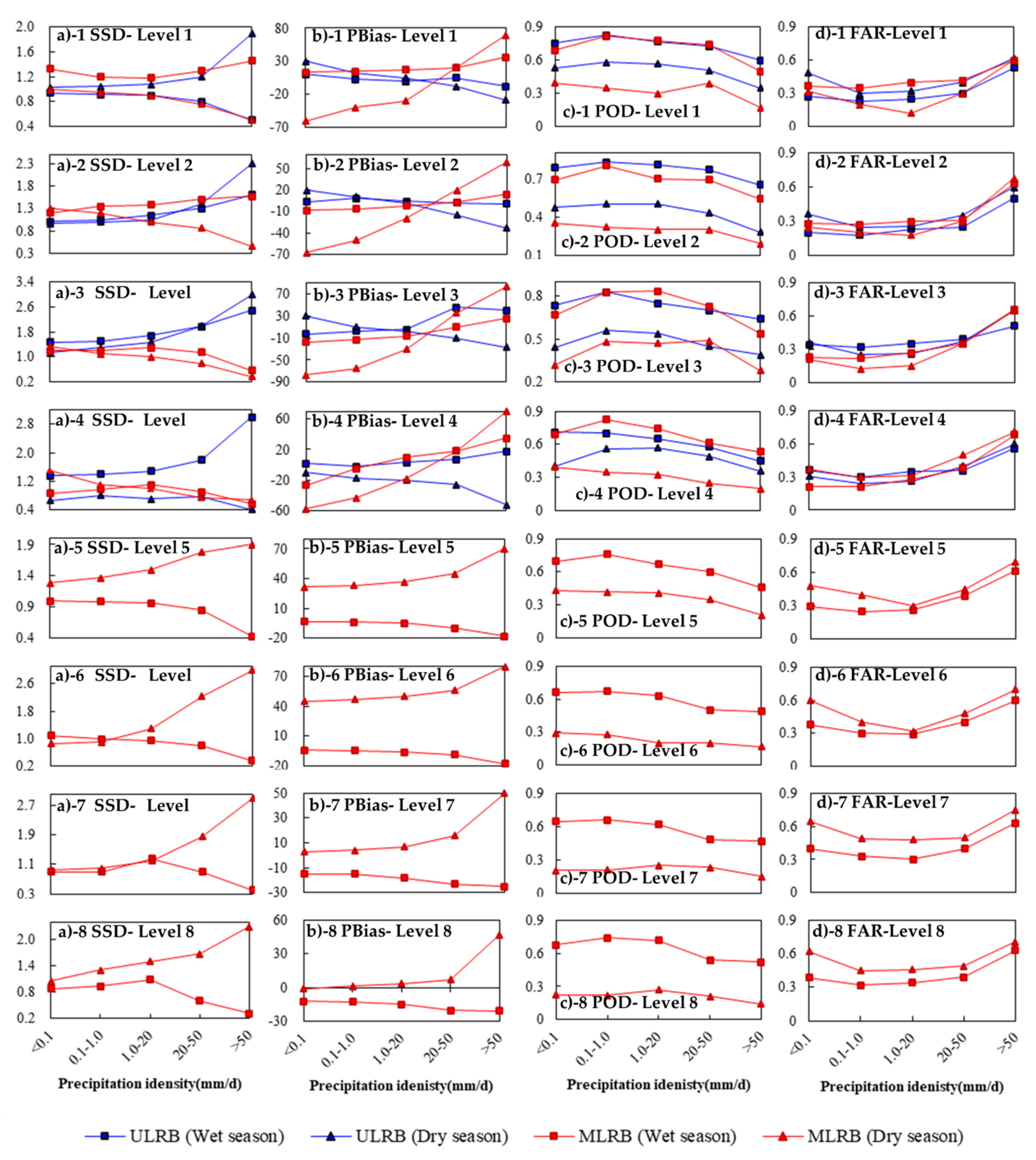
Table 1.
The satellite precipitation estimations used in this study.
| Temporal Extent | Resolutions | Coverage | Description | |
|---|---|---|---|---|
| IMERG E | January 2015–Demcember 2017 | 0.1°/30 min | 60° N–60° S | PMW+IR. Forward propagation. Near real–time (4 h) |
| IMERG L | January 2015–December 2017 | 0.1°/30 min | 60° N–60° S | PMW+IR. Backward and forward propagation. Near real–time (12 h) |
| IMERG F | January 2015–December 2017 | 0.1°/30 min | 60° N–60° S | PMW+IR. monthly GPCC gauge analysis. Post real–time (3.5 months) |
Table 2.
List of indexes used to quantify the performance of satellite precipitation estimations.
| Metrics | Index Type | Index Name | Equation | Unit | Perfect Score |
|---|---|---|---|---|---|
| Amplitude consistency | Statistical index | Correlation coefficient (CC) | NA | 1 | |
| Root mean square error (RMSE) | mm | 0 | |||
| The standard deviation (SD) | mm | 1 | |||
| Percentage of bias (PBias) | NA | 0 | |||
| Occurrence consistency | Classification index | The detection probability (POD) | NA | 1 | |
| The false alarm ratio (FAR) | NA | 0 | |||
| The frequency deviation (FB) | NA | 0 | |||
| The critical success index (CSI) | NA | 1 |
, , is the standard deviation of the gauge observation value. O is the precipitation observation value of the rain gauge, S is the precipitation detection value of IMERG, and n is the total number of samples, . m is the average value of precipitation; A is the number of precipitation events observed by satellites and gauges at the same time. B is the number of precipitation events observed by satellites but not by gauges. C is the number of precipitation events observed by gauges but not by satellites. D is IMERG the number of times the precipitation is observed and the precipitation did not actually occur (Table 3).
Table 3.
Contingency table between the gauge observations and IMERG estimates.
| IMERG | |||
| ≥0.1 mm | <0.1 mm | ||
| Rain Gauge | rain gauge observations ≥ 0.1 mm | A | C |
| rain gauge observations < 0.1 mm | B | D | |
Table 4.
Classification of different rainfall intensity.
| Rainfall Intensity | No Rain | Light Rain | Moderate Rain | Heavy Rain | Extreme Rainfall |
|---|---|---|---|---|---|
| Range (mm/d) | (0–0.1) | (0.1–1) | (1–20) | (20–50) | (>50) |
Table 5.
UMLRB regionalization.
| Zone Name | Latitude | Elevation | Climate Zone | Topographic Area | |
|---|---|---|---|---|---|
| ULRB | River Source Basin (ULRB I) | 31 to 32.9 (°N) | 3801 to 6458 (m) | Alpine Climate Region (no clear distinction between dry and wet seasons) | Plateau Area (high elevation) |
| Zaduo–Changdu Basin (ULRB II) | |||||
| MLRB | Alpine Canyon Basin (MLRB I) | 25.4 to 31 (°N) | 1130 to 6458 (m) | Climate Transition Zone (dry and wet seasons are distinct) | Alpine Canyon Area (great difference in elevation) |
| Mid–high Mountain Canyon Basin (MLRB II) | |||||
Publisher’s Note: MDPI stays neutral with regard to jurisdictional claims in published maps and institutional affiliations. |
© 2021 by the authors. Licensee MDPI, Basel, Switzerland. This article is an open access article distributed under the terms and conditions of the Creative Commons Attribution (CC BY) license (https://creativecommons.org/licenses/by/4.0/).
Share and Cite
MDPI and ACS Style
Lu, C.; Ye, J.; Fang, G.; Huang, X.; Yan, M. Assessment of GPM IMERG Satellite Precipitation Estimation under Complex Climatic and Topographic Conditions. Atmosphere 2021, 12, 780. https://doi.org/10.3390/atmos12060780
AMA Style
Lu C, Ye J, Fang G, Huang X, Yan M. Assessment of GPM IMERG Satellite Precipitation Estimation under Complex Climatic and Topographic Conditions. Atmosphere. 2021; 12(6):780. https://doi.org/10.3390/atmos12060780
Chicago/Turabian StyleLu, Chengxuan, Jian Ye, Guohua Fang, Xianfeng Huang, and Min Yan. 2021. "Assessment of GPM IMERG Satellite Precipitation Estimation under Complex Climatic and Topographic Conditions" Atmosphere 12, no. 6: 780. https://doi.org/10.3390/atmos12060780
Note that from the first issue of 2016, this journal uses article numbers instead of page numbers. See further details here.