
Multi-Decadal Variability and Future Changes in Precipitation over Southern Africa
by
 , , and
Kenny Thiam Choy Lim Kam Sian
1,2,* ,
,
Jianhong Wang
2,
Brian Odhiambo Ayugi
2,3,4,
Isaac Kwesi Nooni
1 and
and
Victor Ongoma
5 
1
Binjiang College, Nanjing University of Information Science and Technology, Wuxi 214105, China
2
Key Laboratory of Meteorological Disaster of Ministry of Education (KLME)/Joint International Research Laboratory of Climate and Environment Change (ILCEC)/Collaborative Innovation Center on Forecast and Evaluation of Meteorological Disasters (CIC-FEMD), Nanjing University of Information Science and Technology, Nanjing 210044, China
3
Jiangsu Key Laboratory of Atmospheric Environment Monitoring and Pollution Control, Collaborative Innovation Center of Atmospheric Environment and Equipment Technology, School of Environmental Science and Engineering, Nanjing University of Information Science and Technology, Nanjing 210044, China
4
Organization of African Academic Doctors (OAAD), Off Kamiti Road, Nairobi P.O. Box 25305-00100, Kenya
5
International Water Research Institute, Mohammed VI Polytechnic University, Lot 660, Hay Moulay Rachid, Ben Guerir 43150, Morocco
*
Author to whom correspondence should be addressed.
Atmosphere 2021, 12(6), 742; https://doi.org/10.3390/atmos12060742
Submission received: 10 May 2021
/
Revised: 31 May 2021
/
Accepted: 4 June 2021
/
Published: 9 June 2021
(This article belongs to the Special Issue Historical and Future Changes in Sub-Saharan African Climate)
Abstract
:The future planning and management of water resources ought to be based on climate change projections at relevant temporal and spatial scales. This work uses the new regional demarcation for Southern Africa (SA) to investigate the spatio-temporal precipitation variability and trends of centennial-scale observation and modeled data, based on datasets from the sixth phase of the Coupled Model Intercomparison Project (CMIP6). The study employs several statistical methods to rank the models according to their precipitation simulation ability. The Theil–Sen slope estimator is used to assess precipitation trends, with a Student’s t-test for the significance test. The comparison of observation and model historical data enables identification of the best-performing global climate models (GCMs), which are then employed in the projection analysis under two Shared Socioeconomic Pathways (SSPs): SSP2-4.5 and SSP5-8.5. The GCMs adequately capture the annual precipitation variation but with a general overestimation, especially over high-elevation areas. Most of the models fail to capture precipitation over the Lesotho-Eswatini area. The three best-performing GCMs over SA are FGOALS-g3, MPI-ESM1-2-HR and NorESM2-LM. The sub-regions demonstrate that precipitation trends cannot be generalized and that localized studies can provide more accurate findings. Overall, precipitation in the wet and dry seasons shows an initial increase during the near future over western and eastern SA, followed by a reduction in precipitation during the mid- and far future under both projection scenarios. Madagascar is expected to experience a decrease in precipitation amount throughout the twenty-first century.
1. Introduction
Climate change is among the top global concerns at present. In recent decades, climate shift and its associated climate dynamics have resulted in increased instability of weather and climate patterns [1,2,3]. Sustainable development requires up-to-date knowledge to make informed decisions and develop strategies based on possible future climate scenarios. Southern Africa (SA) is one of the regions that are very vulnerable to the effects of climate variability and change. The region has experienced large climatic fluctuations during the past century, with distinct variability at different time scales [4,5]. According to Barros et al. [6], SA is highly susceptible to climate change due to its large population, small adaptive ability, poor economic conditions and high exposure. Precipitation over this region is highly variable due to its varying topography and large longitudinal and latitudinal span [7,8,9]. Moreover, the precipitation trend over SA is complex since the area is bordered by the Atlantic and Indian Oceans to the west and east, respectively [10,11,12]. The SA community, like many other parts of Africa, predominantly rely on precipitation-dependent sectors such as agriculture for daily livelihood [13,14,15,16]. Thus, understanding the precipitation patterns is the crux of the matter to establish early warning systems and design mitigation and adaptation strategies for climate change.
The north-to-south oscillation of the tropical rain belt (TRB) throughout the year greatly influences precipitation over the region [17]. The TRB is associated with heavy precipitation to SA during the austral summer [17,18], when the TRB crosses the equator into the Southern Hemisphere. The transition months of April and November contribute to a significant amount of precipitation as well. The austral winter season (May to October) records the lowest amount of precipitation. The semi-permanent anticyclones, the St. Helena High and the Mascarene High, also significantly influence the region’s precipitation [19,20]. Further, some studies [8,21] argue that Rossby waves potentially affect precipitation changes over the SA region through the eastward shift of the South Indian Convergence Zone (SICZ). Besides, other studies have attributed seasonal changes in precipitation to the influence of large-scale atmospheric teleconnections, such as the El Niño-Southern Oscillation (ENSO) and Indian Ocean Dipole (IOD) (e.g., [5,19,22,23]).
Historical precipitation over SA shows seasonal variability, characterized by more pronounced spatial variability than temperature [24]. The strong inter-annual fluctuations in precipitation, with recurring wet and dry periods, are mainly attributed to the response of the coupled ocean-atmosphere modes of variability over the Pacific, Indian and Atlantic Oceans [23]. For instance, the region has experienced a drying trend during austral autumn since the 1970s, predominantly during April and May, resulting from the poleward expansion of the tropical belt [25]. The historical and projected temperature changes show warming tendencies at 0.04 °C/decade in some regions, and higher than 0.2 °C/decade mainly over the southwestern and northeastern parts of the study domain [26]. Thus, SA is regarded as a climate change hotspot [27]. Several studies (e.g., [4,25,28,29]) have pointed to exacerbating situations, with an overall decrease in SA seasonal precipitation over the last century. However, SA’s large zonal and meridional extent leads to significant differences in local precipitation characteristics. An area average of the whole of SA might not accurately describe the actual precipitation changes. Therefore, it is essential to conduct region-based studies. In a recent study, Almazroui et al. [30] used the entire SA domain to determine precipitation trends. Similarly, Cook et al. [31], in a global study on the projection of droughts, reported a likelihood of precipitation reduction over the entirety of SA. However, the sixth Intergovernmental Panel on Climate Change (IPCC AR6) report [1] proposes that SA can be divided into three distinct regions [32] based on the spatial homogeneity of climate characteristics obtained from new observation and modeled datasets.
There is a need for reliable data that projects possible future climate, given the growing awareness of a changing climate. The Coupled Model Intercomparison Project (CMIP) [33], coordinated by the World Climate Research Program (WCRP), is the body responsible for collecting and archiving climate model outputs from different modeling centers and making them publicly available in a standardized format. The CMIP data have become a fundamental tool in climate studies [34]. Over the last few decades, more relevant physical processes have been integrated into the models to reflect the climate system’s natural variability [35]. Precipitation projection studies over SA are mainly based on the CMIP3 and CMIP5 datasets (CMIP Phases 3 and 5). The latest CMIP phase, the CMIP6 dataset [36], uses an updated coupled atmosphere-ocean general circulation model (AOGCM) version and Earth systems model (ESM) simulations of the global climate, grouped under the umbrella term global climate models (GCMs) [35,37]. The GCMs provide improved data to the scientific community for more reliable climate studies.
Apart from improved representation of physical processes, the CMIP6 dataset differs from the Phase 3 and Phase 5 datasets in forcing scenarios and carbon emissions. It applies a new set of Shared Socioeconomic Pathway (SSP) scenarios. The CMIP6 data include historical data and projections based on different SSP scenarios [35,36,38], congruent with the Representative Concentration Pathways (RCPs) of the CMIP3 and CMIP5 via shared policy assumptions.
Accurate prediction of precipitation trends has theoretical and practical significance for agricultural production, household and industrial water use, and hydrological applications, among others [39]. Although several studies have been done over SA, few studies employed the CMIP6 dataset to depict possible future precipitation patterns over the region. Moreover, this work is the first to employ the new regional demarcations for SA. The region-based analysis is in line with the latest application of the Stochastic Rainfall Generator (SRG), which gives users room to carry out an in-depth investigation [40]. This study uses observation and model data to explore the ability of CMIP6 GCMs to simulate precipitation variability. Further, the work investigates how precipitation variability and trends will change over SA throughout the twenty-first century. The ranking of models and the use of ensemble mean of the models address the reliability of model projections supported in the application of SRG [40,41,42].
This paper contributes valuable insights into the precipitation spatio-temporal characteristics over SA, and its new regional demarcations (Section 2.1), based on observation and model data (Section 2.2). This study serves as a critical knowledge transfer. From this perspective, the study aims to investigate the precipitation variability (Section 3.1) and trends (Section 3.2). We also evaluate the model performance and rank the GCMs (Section 3.3), and we investigate the projected precipitation changes (Section 3.4). The methods are introduced in Section 2.3.
2. Materials and Methods
2.1. Study Area
This study is conducted over Southern Africa (SA), which is located between 10–35° S and 10–50° E (Figure 1). The region covers a vast catchment area with extensive coastlines that stretch from the Atlantic Ocean in the west to the Indian Ocean in the east and meet at the Cape Agulhas in the south. The domain covers eleven countries: Angola, Namibia, Zambia, Malawi, Zimbabwe, Botswana, South Africa, Lesotho, Eswatini, Mozambique and Madagascar. The complex and heterogeneous topography possesses extensive mountain ranges, with major lakes and rivers interspaced. The area’s elevation increases from the east to the west. These high-elevation areas act as a natural barrier, preventing wind from directly intruding over the continent [43]. The climate has a strong seasonal characteristic, and the major climate zones according to the Köppen–Geiger classification are tropical, temperate and arid [44,45]. According to Iturbide et al. [32], the new regional demarcations for the SA region are distinguished as Western Southern Africa (WSAF), Eastern Southern Africa (ESAF) and Madagascar (MDG), as shown in Figure 1.
2.2. Data
This study employs three rain gauge-based (observation) gridded datasets and 23 CMIP6 datasets to understand precipitation variability and trends over SA.
2.2.1. Observation Data
Gridded rain gauge-based data are used in place of observational data that is of limited quality and time span. This study uses the Global Precipitation Climatology Centre (GPCC) [47,48] monthly precipitation data version 2018 [49] to compare the observed and simulated precipitation over the region. It has a period of 1891–2016 and a spatial resolution of 0.5° × 0.5°. To assess the observational uncertainties in the GPCC data, we use two other monthly precipitation datasets developed by different centers: Climatic Research Unit (CRU) and University of Delaware (UDEL). The CRU version 4.04 [50,51] provides monthly precipitation data produced at a spatial resolution of 0.5° × 0.5° from 1901 to 2019. We also utilize the UDEL v5.01 monthly precipitation data [52,53], which have a 0.5° × 0.5° horizontal grid resolution and span from 1900 to 2017.
2.2.2. Model Data
We use daily precipitation data from 23 CMIP6 GCMs [36,54]. These datasets run from 1850 to 2100 but with varying spatial resolutions. Table 1 provides the model names, institutions and countries, and horizontal resolutions of all the models. Since the CMIP6 models have different numbers of ensemble members, this work considers all the models’ first member variation rli1p1f1 (r1: realization index, i1: initialization index, p1: physics index, and f1: forcing index). The precipitation projection from the 23 CMIP6 GCMs is analyzed under two representative SSP scenarios: intermediate (SSP2-4.5) and high (SSP5-8.5) forcing scenarios. The SSP2-4.5 is the closest representation of the current efforts being put in place by nations to curb the spiraling emissions of greenhouse gases in the climate system [37]. We also chose SSP5-8.5, the worst possible scenario. Eyring et al. [36] provide details on CMIP6 data.
2.3. Methodology
This study applies a common historical period of 1901–2014 for consistency due to the different periods of the datasets. For the projection, the entire available period (2015–2100) is used. The CMIP6 daily precipitation data are converted to monthly accumulated precipitation to match the temporal scale of the three observation datasets. All the data are re-gridded to a standard 1° × 1° resolution grid. Past studies used a similar re-gridding procedure over Africa (e.g., [30,55,56,57]). The study adopts the upcoming sixth assessment report (AR6)’s [1] recommended baseline period (1995–2014) to calculate the seasonal anomalies relative to the reference data.
We evaluate the GCMs’ ability to replicate the annual and seasonal precipitation variability and trends. The Taylor diagram, Taylor skill score (TSS) and inter-annual variability score (IVS) are used to provide a quantitative performance measure for the data to be used in projection. The data are also ranked using those metrics, thus increasing the confidence of the climate projection results.
The projected monthly precipitation is investigated under two scenarios: SSP2-4.5 and SSP5-8.5 [58]. Three time slices are defined for the projection trend analysis: near future (2015–2044), mid-future (2045–2074) and far future (2075–2100). Precipitation trends are also examined for a continuous period from 2015 to 2100.
2.3.1. Model Performance and Ranking
This study uses the Taylor diagram [59] to give a statistical summary of the model datasets. The Taylor diagram graphically portrays the relationship between the reference (observation) and model datasets, and quantifies the temporal agreement of the different datasets. We select the following statistical metrics: correlation coefficient (R), unbiased root-mean-square difference (ubRMSD) and standard deviation (STD). R measures the similarities in the variability of the reference and simulated data. Its value ranges from −1 to 1, where −1 represents an opposite relationship, 0 means no correlation, and 1 indicates perfect correlation. The RMSD shows how far the model data are from the reference, and portrays uncertainties in both spatial pattern and annual cycle [60]. By totaling the degree of the difference between model and reference, RMSD is a measure of accuracy. The smaller the RMSD value, the closer the model data are to the reference, where 0 is the perfect score. STD portrays the variability in a dataset by showing the distance between each value and the mean of the data. The smaller the STD value, the smaller the dispersion of the values in the dataset is.
We also employ the TSS (Equation (1) [59,61]) to rank the model datasets in their ability to simulate precipitation over SA relative to the reference data. The TSS is a statistical summary of R, RMSD and STD, thus providing a single-value metric. The robustness of the abovementioned technique has been ascertained in previous studies (e.g., [57,62,63]).
where R is the correlation coefficient between reference and model data, σm and σr are the model and reference standard deviations, respectively, and R0 is the highest achievable correlation coefficient (we use a threshold of 0.999). The ideal TSS score is 1.
We calculate the IVS (Equation (2) [60]) to evaluate the model temporal performance relative to the reference data. The IVS complements the TSS by showing the model’s inter-annual variation simulation capability. Past studies have utilized this technique to rank model performance [62,64,65].
The smaller the IVS value, the closer the model’s temporal variability is to the reference data.
2.3.2. Trend Analysis
The Theil–Sen slope estimator (Equation (3) [66]) is applied to the model and reference datasets to quantify the precipitation trend.
where ∆σ is the gradient between two data points in the time series. xj and xk are the corresponding data values for time points j and k (j > k), respectively. We use the median instead of the mean to minimize the influence of outliers on the results. If ∆σ > 0 (∆σ < 0), the trend is increasing (decreasing). A Student’s t-test is applied to test the significance of the results relative to the reference data. Several recent studies (e.g., [67,68,69,70]) have adopted this kind of technique to analyze the trend of hydrometeorological variables based on its robustness in handling the outliers in a time series.
3. Results and Discussion
3.1. Climatology
Figure 2 shows the annual cycle of the observed and modeled precipitation, averaged from 1901 to 2014, over WSAF, ESAF, MDG and SA. The four regions generally show a similar precipitation pattern. MDG records the highest precipitation amount compared with WSAF and ESAF, while ESAF is wetter than WSAF. The precipitation amount gradually increases from July (August) for ESAF and SA (WSAF), and then peaks in January before decreasing again. MDG displays a slight difference in the precipitation minimum, increasing sharply from September, peaks in January and then reduces gradually. The annual variation points to December to March (DJFM) as the wet season over SA [71], while May to October (MJJASO) are the dry months. This work focuses on the two seasons: DJFM and MJJASO. The movement of the TRB modulates this unimodal precipitation pattern.
The CMIP6 ensemble consistently overestimates precipitation as compared to the observation for WSAF, ESAF and SA, while the annual cycles from model and observation over MDG are very close. Moreover, CMIP6 shows a greater degree of deviation, especially in the wet season, portrayed by the large spread of the data around the ensemble mean. The three rain gauge-based datasets present an almost comparable amount of precipitation throughout the year, except for MDG, which shows a larger deviation during the dry season than the other three regions. A slight spread is noted in the observation data during the wet months.
Figure A1 shows the spatial distribution of accumulated precipitation over SA. The annual precipitation distribution (Figure A1a–d) shows that northern SA, central to northern Mozambique, and Madagascar’s eastern coast receive a larger amount of precipitation. In contrast, the southwestern region receives a very low amount of precipitation. Relatively high precipitation coincides with the TRB position, affirming that this phenomenon dominates SA’s wet season. Madagascar shows a distinct west–east precipitation distribution, with precipitation amounts multiple times larger on the east than on the west [72,73]. This is due to the orographic effect [43] from the higher elevation along the island’s center (Figure 1). The three rain gauge-based datasets present very similar spatial distributions with slight maximum precipitation amount differences. The CMIP6 models generally overestimate precipitation over the whole of SA, especially over WSAF (Figure 2). Moreover, a high-precipitation area exists around the Lesotho-Eswatini region and northwestern SA, while the precipitation amount on the eastern side of Madagascar is underestimated.
The spatial precipitation distribution for the wet season (Figure A1e–h) shows that this season dominates the region’s precipitation climatology, supporting a similar observation in Figure 3. Similar to the annual climatology, there are high-precipitation areas over northern SA, central to northern Mozambique and eastern Madagascar. The observation data show higher precipitation (500–700 mm) around the Lesotho-Eswatini area, which is overestimated in the model data (750–1000 mm). Moreover, Madagascar’s northwestern area receives more precipitation than the eastern coast, which is different from the observation. The Madagascar region has a complex system with the interaction between ocean and land, and the models cannot accurately reproduce this system.
The spatial distribution of precipitation in the dry season (Figure A1i–l) shows similar patterns in the three observation datasets. The whole region is generally dry, with a higher amount of precipitation received along the eastern coast of Madagascar, the eastern side of SA and the southern coast of South Africa. In contrast, the model data show an overestimation over the whole of SA, especially over eastern SA and South Africa. The considerable amount of precipitation along the eastern coast of Madagascar during the MJJASO season is due to the easterly wind flowing towards the island, rising because of the island’s high elevation and rain on this side of the island. This high precipitation amount on the east coast of Madagascar is underestimated in the CMIP6 data. The Lesotho-Eswatini area still presents a higher amount of precipitation from the model as compared to the observation. During both the dry and wet seasons, a considerable amount of precipitation can be observed around Angola. The precipitation over this region is influenced by moisture influx from the Congo Rainforest. In the CMIP6 DJFM distribution, this large precipitation area extends further southward over the Kalahari Desert.
We further evaluate the models’ ability to represent the spatial features of precipitation (Figure 3) during the dry and wet seasons, as well as annually. For the annual spatial distribution (Figure 3a–d), the three observation datasets are generally in agreement. GPCC and UDEL present similar spatial distributions with differences in the magnitude of the anomalies. They have an anomaly range between −45 and 57 mm, and −54 and 48 mm, respectively. CRU shows a more homogeneous distribution with positive anomalies (>9 mm) over most of the study domain. There is a negative anomaly (>−13 mm) area over central South Africa, central Madagascar and Angola. The CMIP6 ensemble spatial distribution shows a remarkable overestimation over the whole region, which is more pronounced over the Lesotho-Eswatini area. In contrast, a considerable underestimation is noted along Madagascar’s east coast.
Analyzing the DJFM seasonal anomaly spatial distribution (Figure 3e–h), a similar pattern to that of the annual spatial distribution is observed. This means that the wet season signal dominates the region’s precipitation variability. The CMIP6 DJFM seasonal anomaly shows an even larger magnitude. Also, the underestimation along Madagascar’s east coast still exists. The positions of the large biases in the DJFM spatial distribution co-locate with high-elevation areas in SA (such as the Lesotho-Eswatini area, west Angola, Zambia and Zimbabwe). This suggests that the observed biases might be attributed to the representation of orographic processes in the models.
During the MJJASO season (Figure 3i–l), GPCC and UDEL show more and larger anomaly areas than CRU. The CRU data present mostly positive anomalies, except over Angola and a few other areas. The CMIP6 ensemble still overestimates precipitation over most of SA, with underestimation observed along Madagascar’s east coast and the Cape of Good Hope. Also, the overestimation is more pronounced around the Lesotho-Eswatini area. This area is sensitive and not well simulated by the GCMs during both the wet and dry seasons.
It is notable that the CMIP6 ensemble barely displays negative anomalies over SA. Furthermore, the observation data do not agree over Madagascar during both seasons, implying that this region has a complex system that is not easily captured by the observation datasets.
Overall, the three observation datasets have similar precipitation patterns (Figure 3 and Figure A1), giving more confidence in the results and enabling more robust conclusions about precipitation trends during the past century. The model data match observation to some extent but generally overestimate precipitation, especially during the dry season. Moreover, in both seasons, the Lesotho-Eswatini area is a challenge for the GCMs.
The spatial distribution of seasonal precipitation anomaly from individual models is displayed in Figure A2 and Figure A3 for wet and dry seasons, respectively. The results show that several models have large wet biases over the whole SA region. These models influence the spatial distribution of the CMIP6 ensemble to simulate such large wet anomalies.
3.2. Trend Analysis
The precipitation trends over SA during the DJFM and MJJASO seasons are presented in Figure 4 and Figure 5, respectively. First, the observation and CMIP6 ensembles present similar spatial patterns during the wet season (Figure 4). There is a positive trend over western South Africa, along the Namibian coast, and over northern Mozambique and central Madagascar. The precipitation trend over the rest of the study domain is negative. The individual models show varying spatial distributions, some of which agree with the observation to some extent, such as CNRM-CM6-1, CNRM-ESM2-1, EC-Earth3-Veg, HadGEM3-GC31-LL, GFDL-CM4 and UKESM1-0-LL. The statistically significant areas vary among different models. The reduction in precipitation over the study region has been attributed to the expansion of the sub-tropical dry zone [25]. The results demonstrate the difficulties of simulating the precipitation variability over SA accurately. The influence of the Atlantic and Indian Oceans and forcing from the St. Helena High and Mascarene High influence the model outputs. According to Chen and Xu [74], areas with the same precipitation trend are possibly teleconnected through oceanic forcing. The drying trend over the Eastern Cape region of South Africa corroborates recent research findings over the area [28]. The model ensemble displays an improved spatial trend that closely matches that of observation. Overall, the observation and model ensembles show areas of mixed trends over SA.
The spatial trend of MJJASO precipitation over SA is shown in Figure 5. A comparison of the CMIP6 and the observation ensemble shows that the models do not reproduce the spatial tendency of MJJASO precipitation well. The CMIP6 ensemble shows a significant negative trend over the study domain, while the observation ensemble has mixed trends. Further, the observations do not totally agree with each other over some areas, such as WSAF. The spatial distribution in GPCC is the closest to the observation ensemble, while CRU (UDEL) displays positive trends over WSAF (central SA). The CRU precipitation dataset contains data inhomogeneities that can affect the trend analysis result [50]. None of the models display a pattern close to the observations, highlighting the models’ inability to capture the trend in the dry season.
DJFM and MJJASO precipitation trends is calculated over WSAF, ESAF, MDG and SA (table not shown). Most regions show negative trends except for WSAF, with observations depicting insignificant reductions across all sub-regions. Contrarily, UDEL shows a negative trend at −0.392 over WSAF during DJFM season, while the rest of the observational datasets depict positive trends at 0.023 (0.076) for GPCC (CRU). The inability of CRU to demonstrate a clear tendency is depicted over the SA region, with persistent positive trends being exhibited during both seasons over MDG, while other observations show negative trends. Interestingly, most models show declining patterns in precipitation over most parts of SA. The reduction in precipitation is visible during both seasons.
Overall, the observation and model spatial distributions show varying tendencies. Some models show positive trends while others exhibit negative patterns over different regions. The results demonstrate the challenges for models in simulating precipitation, especially during the dry season. Numerous studies have pointed out this challenge of simulating precipitation compared with temperature over different parts of Africa [75,76,77]. This is mainly associated with issues related to model parameterization, especially in regions with complex physiographical features such as the SA region, or challenges related to local mesoscale features such as lakes, vegetation cover and extensive coastline that cause regional heterogeneity [78]. Furthermore, studies that examined moderate to extreme precipitation noted the observational uncertainties presented herein [79,80]. In fact, Alexander et al. [81] demonstrated that discrepancies between observation datasets are intensified in estimating precipitation extremes, such as consecutive dry days over regional and global domains. In conclusion, Bador et al. [55] and Alexander et al. [81] recommend the use of an observational ensemble derived from various gauge-based sources to assess observational uncertainties better. In this study, the performance demonstrated by GPCC gives the needed confidence to employ this dataset as the reference data in model evaluation to identify the best-performing CMIP6 models for projection analysis.
3.3. Model Performance and Ranking
We use the Taylor diagram, TSS and IVS to assess the capability of individual GCMs in simulating monthly precipitation over the study region and to identify the best-performing GCMs by ranking the models relative to GPCC data.
From the Taylor diagram (Figure 6), the models are clustered in a correlation coefficient range of 0.87 to 0.94, with a ratio of standard deviation between 0.96 and 1.67, and an RMSD of approximately 0.4 to 0.8. Although the temporal variability of precipitation matches GPCC well, the modeled precipitation is usually overestimated. The large overestimation shown by most GCMs confirms the excess precipitation observed in Section 3.1. Out of the 23 GCMs, only Centre National de Recherches Météorologiques’ two models, CNRM-CM6-1 and CNRM-ESM2-1, display an underestimation of precipitation. Further, it is observed that the CMIP6 ensemble presents an improved result with higher R and smaller RMSD.
Since the Taylor diagram is a pictorial representation of three (3) statistical metrics, we employ the TSS, which combines those three metrics and presents a single-value criterion for model performance evaluation and ranking. Moreover, the IVS is also implemented to complement the information provided by the TSS.
We rank the precipitation datasets for each of the following five criteria: STD, R, RMSD, TSS and IVS (Figure 7a). In principle, datasets that portray more blueish color for the five criteria mean that they have good performance for all the statistical metrics considered in this section. Models such as ACCESS-CM2, ACCESS-ESM1-5, BCC-CSM2-MR, CanESM5, EC-Earth3-Veg, GFDL-ESM4, HadGEM3-GC31-LL, INM-CM4-8, INM-CM5-0, IPSL-CM6A-LR, MIROC6, MIROC-ES2L, MRI-ESM2-0 and NESM3 have low ranking throughout by displaying more reddish tones, while models such as CNRM-CM6-1, CNRM-ESM2-1, FGOALS-g3, GFDL-CM4, MPI-ESM1-2-HR, MPI-ESM1-2-LR, NorESM2-LM, NorESM2-MM and UKESM1-0-LL show satisfactory simulation performance. Furthermore, only GFDL-CM4 presents a good ranking for all five metrics.
A scatter plot of TSS against IVS (Figure 7b) displays the different models’ skills in simulating spatial and temporal precipitation patterns over SA. Models with lower IVS and higher TSS are the best-performing. For the projections, models with a TSS (IVS) of less (more) than 0.87 (0.2) are not considered. This assessment provides the confidence for future climate results. The three best- and worst-performing models in our case are the FGOALS-g3, MPI-ESM1-2-HR and NorESM2-LM, and CanESM5, IPSL-CM6A-LR and NESM3, respectively. In addition to the three best-performing models, all GCMs that satisfy the 0.87 and 0.2 thresholds for TSS and IVS, respectively, are used for projection analysis. The models that are kept for projection analysis are the CNRM-CM6-1, CNRM-ESM2-1, FGOALS-g3, GFDL-CM4, MPI-ESM1-2-HR, MPI-ESM1-2-LR, NorESM2-LM, NorESM2-MM and UKESM1-0-LL, which agrees with the ranking in Figure 7a. Moreover, the CMIP6 ensemble ranks highly for the five metrics and shows a clear improvement from the 23 GCMs in the scatter plot. Therefore, the ensemble mean can amply represent the precipitation variability and trend in the projection analysis.
3.4. Projected Precipitation Changes
The nine best-performing models over the study area are used in the projection analysis. We first display the spatial distribution of seasonal precipitation anomalies. We also present the temporal and spatial precipitation trends and the probability density function.
Seasonal precipitation anomaly projections over 2015–2100 under the SSP2-4.5 and SSP5-8.5 scenarios are given in Figure 8. In DJFM (Figure 8a–h), the region exhibits mostly negative values, with positive values moving northwestward. The distribution shows pronounced positive values over the coast of Angola, the Lesotho-Eswatini area and Madagascar’s east coast, while areas such as Mozambique and southeastern South Africa show strong negative anomalies. Dry anomalies are also evident over the entire area during MJJASO (Figure 8i–p) under the SSP2-4.5 and SSP5-8.5 scenarios. Similar to the DJFM distribution, Madagascar also presents positive anomalies over its eastern coast, extending further inland during the dry season than in the wet season.
The persistent dry anomaly over ESAF and MDG compared with WSAF could be attributed to higher pressure, warmer SSTs in the Pacific Ocean, and Indian Ocean offshore winds that lead to decreased precipitation [22]. Drying patterns over the region can have adverse effects on several sectors of the economy, such as agriculture.
Precipitation trends over WSAF, ESAF, MDG and SA during the near, mid- and far future are presented in Figure 9. Notably, the nine GCMs used for the projection analysis have a large spread about the ensemble mean. However, according to Milinski et al. [82], the ensemble helps to reduce uncertainties in the data. The area-averaged projected precipitation variation does not accurately represent projected precipitation over the different sub-regions (WSAF, ESAF and MDG). Therefore, we examine precipitation changes over each of SA’s three sub-regions. The temporal trend depicts periods of positive and negative anomalies. Analyzing the DJFM trends for WSAF (Figure 9a), it is observed that there is a downward trend (−0.213) during the near future for SSP2-4.5, followed by an upward trend (0.639) during the mid-future and a downward trend during the far future (−0.272). The downward trends are approximately a third of the magnitude of the upward trend. On the other hand, the SSP5-8.5 shows continuous negative trends during the three timelines: −0.339, −0.122 and −0.218. The MJJASO trends for WSAF (Figure 9b) show negative trends during the three time sections for both SSP2-4.5 (−0.049, −0.023 and −0.061) and SSP5-8.5 (−0.009, −0.076 and −0.111). The trends over WSAF describe an overall decrease in precipitation in the twenty-first century, except for the mid-future under the moderate forcing scenario. The negative trends in SSP2-4.5 might point to the possibility that WSAF is more significantly influenced by natural variability than anthropogenic factors. However, the SSP5-8.5 trends show that strong anthropogenic forcing promotes precipitation decrease, especially in the dry season.
Under the intermediate forcing scenario, ESAF shows an accelerated wetting tendency (0.683) during the DJFM’s near future followed by a drying tendency during the consecutive two time slices (−0.235 and −0.097) (Figure 9c). On the other hand, the strong forcing scenario (Figure 9d) shows a drying trend (−0.809) during the near future followed by wetting trends during the mid- and far future (0.095 and 0.113). The trends of both scenarios during the near future are quite large relative to the other two time sections. Also, the precipitation trends are opposite under the two scenarios. The trends for MJJASO over the same region (Figure 9d) show a decreasing pattern during the three time slices for the SSP2-4.5 scenarios (−0.023, −0.031 and −0.081). In contrast, the SSP5-8.5 shows an upward trend during the near future (0.041), followed by downward trends during the successive two time slices (−0.063 and −0.0157). It is also observed that the magnitude of the trends for the SSP5-8.5 is about twice that of SSP2-4.5.
Over MDG, the DJFM precipitation trend is upwards (Figure 9e) in the near future, followed by negative trends during the mid-future (−1.294) and positive trends during the far future (0.145). The SSP5-8.5 shows a downward trend during the near future (−0.047), followed by relatively larger negative trends during the mid- and far future (−1.351 and −0.684). The MJJASO precipitation trend over MDG (Figure 9f) shows a drying tendency during the three time slices for both the SSP2-4.5 and SSP5-8.5 scenarios. Moreover, the magnitude of the trends is nearly the same. This observation might indicate that the precipitation over MDG during its dry season is not significantly modulated by anthropogenic forcing. As previously reported, this region is strongly influenced by the ocean [19,23], and thus the effect of climate shift on the area is minimal.
An overview of the changes in precipitation trend over the whole SA study domain under the SSP2-4.5 and SSP5-8.5 scenarios is given in Figure 9g,h. The DJFM season is projected to get wetter in the near (0.362) and mid-future (0.046), followed by a drying tendency during the far future (−0.155). The trends under the strong forcing scenario show a drying pattern throughout the three time slices (−0.548, −0.067 and −0.046). The MJJASO season also displays an overall drying trend during the near, mid- and far future (−0.037, −0.031 and −0.068) under the SSP2-4.5 scenario. The SSP5-8.5 shows a very insignificant downward trend in the near future (0.007), followed by more significant drying trends during the mid- (−0.067) and far future (−0.129). The findings are in agreement with Cook et al. [31], who used 13 CMIP6 models to project droughts over SA in a global study. According to the study, the region is expected to experience drying patterns in precipitation. The study equally projected a reduction in total column soil moisture over SA, which threatens agriculture in the region.
In summary, the DJFM precipitation is projected to decrease under the SSP2-4.5, but is depressed under the SSP5-8.5 over areas such as WSAF and MDG. On the other hand, MJJASO presents a mostly unanimous display of decreasing trends over the three sub-regions and under both scenarios, which means that the natural variability of the region is already in the dry phase. Also, SA’s trends and magnitudes highlight the importance of conducting region-based analysis as it is clear that the SA values do not accurately explain the trends over the different sub-regions.
The spatial distribution of DJFM and MJJASO projected precipitation trend is displayed for the near, mid- and far future, under the SSP2-4.5 and SSP5-8.5 scenarios (Figure 10). The DJFM spatial trends under the SSP2-4.5 scenario (Figure 10a–d) show a nearly opposite distribution during the near and mid-future. Most of SA displays a drying tendency during the far future, with a few wetting areas over northern Madagascar, southern South Africa and southern Mozambique. Overall, the continuous period shows a general drying trend, except for the Eswatini area, western Angola and the south tip of Madagascar. The SSP5-8.5 (Figure 10e–h) shows an opposite pattern as compared to SSP2-4.5 during the near future. ESAF displays a general drying trend, and Angola shows a wetting tendency. During the mid-future, the trend changes to positive over ESAF and mostly negative over WSAF. MDG has a positive (negative) trend on its west (east) side. During the far future, most of the SA region is covered with negative trends. A few areas, such as eastern South Africa, southern MDG and western Angola, show a positive trend. The continuous period shows a nearly similar distribution to that of SSP2-4.5.
The MJJASO season (Figure 10i–l) shows a general drying trend during the near future, except for the Lesotho-Eswatini area. During the mid-future, central SA and regions such as northern MDG show positive trends. During the far future, the study domain is again mostly covered with negative trends. Overall, there is a decrease in MJJASO precipitation during the twenty-first century under the moderate forcing scenario. Under the SSP5-8.5 scenario, the MJJASO dry season (Figure 10m–p) shows an overall statistically significant drying trend, especially during the mid- and far future. The southeastern coast of SA proves to be an interesting area as it is the one region showing positive trends under the strong forcing scenario. Overall, there is a drying trend over the whole of SA under the SSP5-8.5. For the analysis of spatial trends, the Lesotho-Eswatini area is shown to be a sensitive region during the next few decades. The precipitation over the entire projection period is consistently statistically significant over WSAF areas, while in the other time slices, the statistical significance varies from region to region.
The probability density function (PDF) of projected precipitation during four reference time sections averaged over WSAF, ESAF, MDG and SA, under the SSP2-4.5 scenario is shown in Figure 11. The DJFM precipitation over WSAF (Figure 11a) shows an increase (~25 mm) during the near future, followed by a slight decrease of ~5 mm during the mid-future, and the far future maintains nearly the same amount of precipitation. The ESAF (Figure 11b) also shows an initial increase during the near future (~15 mm), followed by a drop of ~5 mm during the mid-future, before picking up again by a few mm during the far future. Over MDG (Figure 11c), there is a decrease during the near future (~10 mm), followed by an increase (~5 mm), before decreasing again during the far future. Overall, SA (Figure 11d) displays an initial increase during the near future, before decreasing during the mid-future. The far future presents a nearly similar distribution to the mid-future. The subsequent decrease in precipitation amount during the mid- and far future can be detrimental to rain-fed agriculture. This effect will be amplified over MDG as the precipitation amount is anticipated to decline in the near future.
During the MJJASO season, the distribution over WSAF (Figure 11e) shows an increase relative to the baseline period during the near future, followed by a decrease during the mid-future and a further decrease during the far future. The ESAF (Figure 11f) also shows a similar pattern to that of WSAF. That is, an increase during the near future, followed by a decrease during the successive time sections. MDG (Figure 11g), on the other hand, shows a continuous decline throughout the three time sections. Overall, MJJASO precipitation under the SSP2-4.5 shows an initial increase over SA during the near future, followed by a decline during the mid- and far future.
Figure 12 shows the PDF for DJFM and MJJASO under the SSP5-8.5 scenario. During the near future, there is an increase in DJFM precipitation over WSAF, ESAF and SA, while MDG experiences a precipitation reduction. WSAF (Figure 12a) shows a decreased precipitation amount during the subsequent time slices. In contrast, ESAF (Figure 12b) displays a further increase from the near to mid-future. From the mid- to far future, there is a decrease in precipitation. Over MDG (Figure 12c), precipitation experiences a continuous decrease during the three time sections. Overall, SA (Figure 12d) illustrates an initial increase in precipitation during the near future relative to the baseline period, followed by a reduction during the mid- and far future.
For the MJJASO season, precipitation over WSAF (Figure 12e) shows an increase during the near future from the baseline period. There is a decrease in precipitation during the mid-future, which is further accentuated during the far future, reaching an amount slightly less than that of the baseline period. The ESAF (Figure 12f) shows a continuous precipitation decrease during the three consecutive time slices after an initial increase during the near future. As observed in the DJFM precipitation, the MJJASO precipitation over MDG (Figure 12g) also experiences a constant decrease throughout the three time slices. Overall, SA (Figure 12) displays an initial increase in precipitation during the near future, followed by precipitation reduction during the mid- and far future.
The results point to a general increase in DJFM and MJJASO precipitation over WSAF and ESAF during the near future, followed by a slight decrease during the subsequent two time sections. In contrast, MDG displays an apparent reduction in precipitation during both seasons. Moreover, the severity of the precipitation reduction is accentuated throughout the twenty-first century.
4. Summary and Conclusions
Climate change is of great interest to the scientific community, policy makers and the general public. Understanding shifts in precipitation variability is crucial for explaining the hydrological cycle response to a natural or forced change in the climate system. A disparity in precipitation could heavily impact SA, where the agricultural sector is a primary source of livelihood. Policy makers require detailed, in-depth information on regional changes in precipitation to devise suitable adaptation and mitigation plans to minimize the devastating effect of such changes in precipitation amount.
By using the new regional demarcations for SA, this study investigates the changes in precipitation variability and trends during the twentieth and twenty-first centuries. We compare the historical data of 23 CMIP6 GCMs against rain gauge-based data (GPCC, CRU and UDEL) to assess the individual models’ performance in simulating annual precipitation variation, seasonal inter-annual variability and trends. We then select the models with good simulation capabilities for the projection analysis. The evaluation statistical metrics are the STD, R, RMSD, TSS and IVS, and the Theil–Sen slope estimator is used for the trend analysis. For the future precipitation projection, two scenarios, SSP2-4.5 and SSP5-8.5, represent the possible current state of the atmosphere and the worst possible situation, respectively.
From the comparison of observation data, it is found that the three datasets agree with each other. GPCC, however, shows more resemblance to the observation ensemble during the dry season. Therefore, we use GPCC as the reference data for model performance evaluation. By comparing the observation data with the model datasets, we note that no single GCM is the most consistent for all three sub-regions. Most of the models overestimate precipitation over the study region and underestimate precipitation along the east coast of Madagascar. The CMIP6 ensemble gives a better representation of precipitation than individual models, which agrees with Pincus et al. [83] and Pierce et al. [84], who reported that ensemble means limit spatial uncertainty and inconsistency. Moreover, GCMs inevitably introduce uncertainties into the projections due to model parameterizations, among other factors. The CMIP6 GCMs cannot well simulate areas of fast-changing topography or high elevation, such as the Lesotho-Eswatini area, the Angola coast and the high topography in the center of Madagascar. ESAF and MDG are also complex areas that the GCMs cannot accurately simulate. The models have limitations in fully representing specific physical processes [35]. Unknown variations in the climate system and inadequate understanding of the climate response over longer timescales [85] also present huge uncertainties. Therefore, it is crucial to interpret these data in light of their uncertainties. Moreover, it is assumed that the current observed shift in climate regime is attributed to human factors. Another school of thought argues that these changes are caused by natural variability in the climate system, thus adding more uncertainties into future projections [86].
In the model evaluation, the Taylor diagram shows that, apart from CNRM-CM6-1 and CNRM-ESM2-1, all other models overestimate precipitation to different degrees. Using the TSS and IVS, we rank the models according to their simulation skills. The five best- and worst-performing models over SA are CNRM-CM6-1, FGOALS-g3, MPI-ESM1-2-HR, NorESM2-LM and NorESM2-MM, and CanESM5, EC-Earth3-Veg, IPSL-CM6A-LR, MIROC6 and NESM3, respectively. A TSS (IVS) threshold of 0.87 (0.2) identifies suitable models for projection analysis. The models selected for projection analysis are CNRM-CM6-1, CNRM-ESM2-1, FGOALS-g3, GFDL-CM4, MPI-ESM1-2-HR, MPI-ESM1-2-LR, NorESM2-LM, NorESM2-MM and UKESM1-0-LL.
Precipitation variability is highly inhomogeneous. Unlike temperature, which displays uniform variation, precipitation shows considerable spatial variability. While past studies described a generalized trend over the whole of SA, this study reports precipitation over WSAF, ESAF and MDG. The results point to a pattern that is not reflected over the whole study region average. A general increase in DJFM and MJJASO precipitation over WSAF and ESAF is expected during the near future, followed by a slight decrease during the subsequent two time sections. Some localized areas are likely to experience increasing trends during the mid- and far future. In contrast, MDG displays a clear decrease in precipitation during both seasons. Moreover, the severity of the precipitation reduction is accentuated throughout the twenty-first century. Overall, the findings on projected precipitation over SA reaffirm the results of previous studies [87,88,89] that were based on CMIP5. Although strategies have been put in place to limit carbon dioxide emissions and to “reverse” the devastating effect of global warming/climate change, the projected trends over SA point to an overall drying pattern over the three sub-regions under the SSP2-4.5. It is therefore imperative to properly manage the available water resources through sound planning.
The introduction of the latest phase of the CMIP data provides an excellent source for studying future precipitation trends over SA. The CMIP6 is an improvement of its predecessors, with a better representation of several physical processes. The SSPs also contribute to a more realistic interpretation of different world situation scenarios, thus giving more confidence in the results presented in this study. In contrast to previous studies that applied a general domain for SA, this study delineates SA into WSAF, ESAF and MDG, providing a more accurate understanding of the precipitation trends over the three regions. It is important to emphasize that the statistical metrics used in this study quantify the relative changes in climate patterns during the twentieth and twenty-first centuries. The results are not to be explained as the magnitude of climate change impact on SA.
This work establishes the trend during the past and future centuries. However, contributing factors such as dynamic mechanisms and processes have not been explored in detail. A further study aims to explore the dynamic aspect of precipitation trends over the different SA regions. Also, the large wet biases displayed by most models require further investigations to understand the models’ physical representations that led to such results.
Author Contributions
Conceptualization, K.T.C.L.K.S. and J.W.; Data curation, K.T.C.L.K.S.; Methodology, K.T.C.L.K.S. and B.O.A.; Resources, K.T.C.L.K.S.; Supervision, J.W.; Validation, K.T.C.L.K.S.; Visualization, K.T.C.L.K.S.; Writing—original draft, K.T.C.L.K.S.; Writing—review and editing, J.W., B.O.A., V.O. and I.K.N. All authors have read and agreed to the published version of the manuscript.
Funding
This research is funded by project number 560120054.
Acknowledgments
The authors are grateful to the developers, managers and funding agencies of CRU, GPPC, UDEL and CMIP6 data for making the data publicly available.
Conflicts of Interest
The authors declare no conflict of interest.
Appendix A
Figure A1.
Spatial distribution of accumulated precipitation climatology (mm) over Southern Africa. (a–d) Annual; (e–h) DJFM; and (i–l) MJJASO precipitation from (a,e,i) GPCC; (b,f,j) CRU; (c,g,k) UDEL; and (d,h,l) CMIP6 ensemble mean.
Figure A1.
Spatial distribution of accumulated precipitation climatology (mm) over Southern Africa. (a–d) Annual; (e–h) DJFM; and (i–l) MJJASO precipitation from (a,e,i) GPCC; (b,f,j) CRU; (c,g,k) UDEL; and (d,h,l) CMIP6 ensemble mean.

Figure A2.
Spatial distribution of DJFM seasonal precipitation anomaly (mm) averaged from 1901 to 2014 over Southern Africa.
Figure A2.
Spatial distribution of DJFM seasonal precipitation anomaly (mm) averaged from 1901 to 2014 over Southern Africa.

Figure A3.
The same as Figure A2, but for the MJJASO season.
Figure A3.
The same as Figure A2, but for the MJJASO season.

References
- IPCC Global Warming of 1.5 °C. An IPCC Special Report on the Impacts of Global Warming of 1.5 °C Above Pre-Industrial Levels and Related Global Greenhouse Gas Emission Pathways, in the Context of Strengthening the Global Response to the Threat of Climate Change; Masson-Delmotte, V., Zhai, P., Pörtner, H.-O., Roberts, D., Skea, J., Shukla, P.R., Pirani, A., Moufouma-Okia, W., Péan, C., Pidcock, R., et al., Eds.; IPCC: Geneva, Switzerland, 2018. [Google Scholar]
- Steffen, W.; Rockström, J.; Richardson, K.; Lenton, T.M.; Folke, C.; Liverman, D.; Summerhayes, C.P.; Barnosky, A.D.; Cornell, S.E.; Crucifix, M.; et al. Trajectories of the Earth System in the Anthropocene. Proc. Natl. Acad. Sci. USA 2018, 115, 8252–8259. [Google Scholar] [CrossRef] [Green Version]
- Ritchie, P.; Clarke, J.; Cox, P.; Huntingford, C. Overshooting Tipping Point Thresholds in A Changing Climate. Nature 2021, 592, 517–523. [Google Scholar] [CrossRef]
- Shongwe, M.E.; Van Oldenborgh, G.J.; Van Den Hurk, B.J.J.M.; De Boer, B.; Coelho, C.A.S.; Van Aalst, M.K. Projected changes in mean and extreme precipitation in Africa under global warming. Part I: Southern Africa. J. Clim. 2009, 22, 3819–3837. [Google Scholar] [CrossRef]
- Morioka, Y.; Engelbrecht, F.; Behera, S.K. Potential sources of decadal climate variability over southern Africa. J. Clim. 2015, 28, 8695–8709. [Google Scholar] [CrossRef]
- Barros, V.R. Coauthors Climate Change 2014 Impacts, Adaptation, and Vulnerability Part B: Regional Aspects: Working Group II Contribution to the Fifth Assessment Report of the Intergovernmental Panel on Climate Change; Cambridge University Press: Cambridge, UK, 2014. [Google Scholar]
- Mason, S.J. Temporal variability of sea surface temperatures around Southern Africa: A possible forcing mechanism for the 18-year rainfall oscillation? S. Afr. J. Sci. 1990, 86, 243–252. [Google Scholar]
- Hart, N.C.G.; Reason, C.J.C.; Fauchereau, N. Cloud bands over southern Africa: Seasonality, contribution to rainfall variability and modulation by the MJO. Clim. Dyn. 2013, 41, 1199–1212. [Google Scholar] [CrossRef]
- Botai, C.M.; Botai, J.O.; Adeola, A.M. Spatial distribution of temporal precipitation contrasts in South Africa. S. Afr. J. Sci. 2018, 114, 70–78. [Google Scholar] [CrossRef]
- Nel, W. Rainfall trends in the KwaZulu-Natal Drakensberg region of South Africa during the twentieth century. Int. J. Climatol. 2009, 29, 1634–1641. [Google Scholar] [CrossRef]
- Cook, K.H.; Vizy, E.K. Projected changes in east african rainy seasons. J. Clim. 2013, 26, 5931–5948. [Google Scholar] [CrossRef]
- Ogwang, B.A.; Chen, H.; Li, X.; Gao, C. The influence of topography on East African October to December climate: Sensitivity experiments with RegCM4. Adv. Meteorol. 2014, 2014. [Google Scholar] [CrossRef]
- Black, E.; Slingo, J.; Sperber, K.R. An observational study of the relationship between excessively strong short rains in coastal East Africa and Indian ocean SST. Mon. Weather Rev. 2003, 131, 74–94. [Google Scholar] [CrossRef]
- Ogallo, L.J.; Oludhe, C. Climate information in decision making in the greater horn of Africa: Lessons and experiences. WMO Bull. 2009, 58, 184–187. [Google Scholar]
- Ogwang, B.A.; Chen, H.; Tan, G.; Ongoma, V.; Ntwali, D. Diagnosis of East African climate and the circulation mechanisms associated with extreme wet and dry events: A study based on RegCM4. Arab. J. Geosci. 2015, 8, 10255–10265. [Google Scholar] [CrossRef]
- Ogwang, B.A.; Chen, H.; Li, X.; Gao, C. Evaluation of the capability of RegCM4.0 in simulating East African climate. Theor. Appl. Climatol. 2016, 124, 303–313. [Google Scholar] [CrossRef]
- Nicholson, S.E. The ITCZ and the seasonal cycle over equatorial Africa. Bull. Am. Meteorol. Soc. 2018, 99, 337–348. [Google Scholar] [CrossRef]
- Dunning, C.M.; Black, E.C.L.; Allan, R.P. The onset and cessation of seasonal rainfall over Africa. J. Geophys. Res. 2016, 121, 11405–11424. [Google Scholar] [CrossRef] [Green Version]
- Morioka, Y.; Takaya, K.; Behera, S.K.; Masumoto, Y. Local SST impacts on the summertime mascarene high variability. J. Clim. 2015, 28, 678–694. [Google Scholar] [CrossRef]
- Xulu, N.G.; Chikoore, H.; Bopape, M.J.M.; Nethengwe, N.S. Climatology of the mascarene high and its influence on weather and climate over Southern Africa. Climate 2020, 8, 86. [Google Scholar] [CrossRef]
- Cook, K.H. The South Indian convergence zone and interannual rainfall variability over Southern Africa. J. Clim. 2000, 13, 3789–3804. [Google Scholar] [CrossRef]
- Reason, C.J.C.; Rouault, M. ENSO-like decadal variability and South African rainfall. Geophys. Res. Lett. 2002, 29, 16-1–16-4. [Google Scholar] [CrossRef] [Green Version]
- Dieppois, B.; Poh, B.; Rouault, M.; New, M.; Lawler, D.; Keenlyside, N. Interannual to interdecadal variability of winter and summer southern African rainfall, and their teleconnections. J. Geophys. Res. Atmos. 2016, 121, 6215–6239. [Google Scholar] [CrossRef] [Green Version]
- Orlowsky, B.; Seneviratne, S.I. Global changes in extreme events: Regional and seasonal dimension. Clim. Chang. 2012, 110, 669–696. [Google Scholar] [CrossRef] [Green Version]
- Cai, W.; Cowan, T.; Thatcher, M. Rainfall reductions over Southern Hemisphere semi-arid regions: The role of subtropical dry zone expansion. Sci. Rep. 2012, 2, 702. [Google Scholar] [CrossRef] [Green Version]
- Kruger, A.C.; Nxumalo, M.P. Historical rainfall trends in South Africa: 1921–2015. Water SA 2017, 43, 285–297. [Google Scholar] [CrossRef] [Green Version]
- Diffenbaugh, N.S.; Giorgi, F. Climate change hotspots in the CMIP5 global climate model ensemble. Clim. Chang. 2012, 114, 813–822. [Google Scholar] [CrossRef] [Green Version]
- Mahlalela, P.T.; Blamey, R.C.; Hart, N.C.G.; Reason, C.J.C. Drought in the Eastern Cape region of South Africa and trends in rainfall characteristics. Clim. Dyn. 2020, 55, 2743–2759. [Google Scholar] [CrossRef] [PubMed]
- Roffe, S.J.; Fitchett, J.M.; Curtis, C.J. Investigating changes in rainfall seasonality across South Africa: 1987–2016. Int. J. Climatol. 2020, 41, 1–20. [Google Scholar] [CrossRef]
- Almazroui, M.; Saeed, F.; Saeed, S.; Nazrul Islam, M.; Ismail, M.; Klutse, N.A.B.; Siddiqui, M.H. Projected Change in Temperature and Precipitation Over Africa from CMIP6. Earth Syst. Environ. 2020, 4, 455–475. [Google Scholar] [CrossRef]
- Cook, B.I.; Mankin, J.S.; Marvel, K.; Williams, A.P.; Smerdon, J.E.; Anchukaitis, K.J. Twenty-First Century Drought Projections in the CMIP6 Forcing Scenarios. Earth Futur. 2020, 8, e2019EF001461. [Google Scholar] [CrossRef] [Green Version]
- Iturbide, M.; Gutiérrez, J.M.; Alves, L.M.; Bedia, J.; Cerezo-Mota, R.; Cimadevilla, E.; Cofiño, A.S.; Di Luca, A.; Faria, S.H.; Gorodetskaya, I.; et al. An update of IPCC climate reference regions for subcontinental analysis of climate model data: Definition and aggregated datasets. Earth Syst. Sci. Data 2020, 12, 2959–2970. [Google Scholar] [CrossRef]
- Meehl, G.A.; Boer, G.J.; Covey, C.; Latif, M.; Stouffer, R.J. The Coupled Model Intercomparison Project (CMIP). Bull. Am. Meteorol. Soc. 2000, 81, 313–318. [Google Scholar] [CrossRef] [Green Version]
- Gates, W.L. AMIP: The Atmospheric Model Intercomparison Project. Bull. Am. Meteorol. Soc. 1992, 73, 1962–1970. [Google Scholar] [CrossRef] [Green Version]
- Stouffer, R.J.; Eyring, V.; Meehl, G.A.; Bony, S.; Senior, C.; Stevens, B.; Taylor, K.E. CMIP5 scientific gaps and recommendations for CMIP6. Bull. Am. Meteorol. Soc. 2017, 98, 95–105. [Google Scholar] [CrossRef]
- Eyring, V.; Bony, S.; Meehl, G.A.; Senior, C.A.; Stevens, B.; Stouffer, R.J.; Taylor, K.E. Overview of the Coupled Model Intercomparison Project Phase 6 (CMIP6) experimental design and organization. Geosci. Model Dev. 2016, 9, 1937–1958. [Google Scholar] [CrossRef] [Green Version]
- Riahi, K.; van Vuuren, D.P.; Kriegler, E.; Edmonds, J.; O’Neill, B.C.; Fujimori, S.; Bauer, N.; Calvin, K.; Dellink, R.; Fricko, O.; et al. The Shared Socioeconomic Pathways and their energy, land use, and greenhouse gas emissions implications: An overview. Glob. Environ. Chang. 2017, 42, 153–168. [Google Scholar] [CrossRef] [Green Version]
- Simpkins, G. Progress in climate modelling. Nat. Clim. Chang. 2017, 7, 684–685. [Google Scholar] [CrossRef]
- IPCC Climate Change 2014: Synthesis Report. Contribution of Working Groups I, II and III to the Fifth Assessment Report of the Intergovernmental Panel on Climate Change; Team, C.W., Pachauri, R.K., Meyer, L.A., Eds.; IPCC: Geneva, Switzerland, 2014. [Google Scholar]
- De Luca, D.L.; Petroselli, A.; Galasso, L. A transient stochastic rainfall generator for climate changes analysis at hydrological scales in central Italy. Atmosphere 2020, 11, 1292. [Google Scholar] [CrossRef]
- Burton, A.; Fowler, H.J.; Blenkinsop, S.; Kilsby, C.G. Downscaling transient climate change using a Neyman-Scott Rectangular Pulses stochastic rainfall model. J. Hydrol. 2010, 381, 18–32. [Google Scholar] [CrossRef]
- Blenkinsop, S.; Harpham, C.; Burton, A.; Goderniaux, P.; Brouyère, S.; Fowler, H.J. Downscaling transient climate change with a stochastic weather generator for the Geer catchment, Belgium. Clim. Res. 2013, 57, 95–109. [Google Scholar] [CrossRef] [Green Version]
- Favre, A.; Hewitson, B.; Lennard, C.; Cerezo-Mota, R.; Tadross, M. Cut-off Lows in the South Africa region and their contribution to precipitation. Clim. Dyn. 2013, 41, 2331–2351. [Google Scholar] [CrossRef]
- Peel, M.C.; Finlayson, B.L.; McMahon, T.A. Updated world map of the Köppen-Geiger climate classification. Hydrol. Earth Syst. Sci. 2007, 11, 1633–1644. [Google Scholar] [CrossRef] [Green Version]
- Engelbrecht, C.J.; Engelbrecht, F.A. Shifts in Köppen-Geiger climate zones over southern Africa in relation to key global temperature goals. Theor. Appl. Climatol. 2016, 123, 247–261. [Google Scholar] [CrossRef]
- NOAA National Geophysical Data Center. 2-minute Gridded Global Relief Data (ETOPO2) v2; NOAA National Centers for Environmental Information: Asheville, NC, USA, 2006. [CrossRef]
- Becker, A.; Finger, P.; Meyer-Christoffer, A.; Rudolf, B.; Schamm, K.; Schneider, U.; Ziese, M. A description of the global land-surface precipitation data products of the Global Precipitation Climatology Centre with sample applications including centennial (trend) analysis from 1901-present. Earth Syst. Sci. Data 2013, 5, 921–998. [Google Scholar] [CrossRef] [Green Version]
- Schneider, U.; Finger, P.; Meyer-Christoffer, A.; Rustemeier, E.; Ziese, M.; Becker, A. Evaluating the hydrological cycle over land using the newly-corrected precipitation climatology from the Global Precipitation Climatology Centre (GPCC). Atmosphere 2017, 8, 52. [Google Scholar] [CrossRef] [Green Version]
- Physical Sciences Laboratory. Global Precipitation Climatology Centre (GPCC) Full Data Reanalysis Version 2018. Available online: https://www.esrl.noaa.gov/psd/ (accessed on 3 December 2020).
- Harris, I.; Osborn, T.J.; Jones, P.; Lister, D. Version 4 of the CRU TS monthly high-resolution gridded multivariate climate dataset. Sci. Data 2020, 7, 109. [Google Scholar] [CrossRef] [PubMed] [Green Version]
- Climatic Research Unit, University of East Anglia. Climatic Research Unit (CRU) TS Version 4.04. Available online: https://crudata.uea.ac.uk/cru/data/hrg/cru_ts_4.04/ (accessed on 14 September 2020).
- Willmott, C.J.; Matsuura, K. Terrestrial Air Temperature and Precipitation: Monthly and Annual Time Series (1950–1999) (Version 1.02). 2001. Available online: http://climate.geog.udel.edu/~climate/html_pages/download.html#ghcn_T_P2 (accessed on 9 June 2021).
- University of Delaware. University of Delaware (UDEL) Precipitation v5.01. Available online: https://psl.noaa.gov/data/gridded/data.UDel_AirT_Precip.html (accessed on 3 December 2020).
- World Climate Research Programme. Coupled Model Intercomparison Project Phase 6 (CMIP6). Available online: https://esgf-node.llnl.gov/search/cmip6 (accessed on 15 January 2021).
- Bador, M.; Boé, J.; Terray, L.; Alexander, L.V.; Baker, A.; Bellucci, A.; Haarsma, R.; Koenigk, T.; Moine, M.-P.; Lohmann, K.; et al. Impact of Higher Spatial Atmospheric Resolution on Precipitation Extremes Over Land in Global Climate Models. J. Geophys. Res. Atmos. 2020, 125, e2019JD032184. [Google Scholar] [CrossRef]
- Iyakaremye, V.; Zeng, G.; Siebert, A.; Yang, X. Contribution of external forcings to the observed trend in surface temperature over Africa during 1901–2014 and its future projection from CMIP6 simulations. Atmos. Res. 2021, 254, 105512. [Google Scholar] [CrossRef]
- Ngoma, H.; Wen, W.; Ayugi, B.; Babaousmail, H.; Karim, R.; Ongoma, V. Evaluation of precipitation simulations in CMIP6 models over Uganda. Int. J. Climatol. 2021, 1–26. [Google Scholar] [CrossRef]
- O’Neill, B.C.; Tebaldi, C.; Van Vuuren, D.P.; Eyring, V.; Friedlingstein, P.; Hurtt, G.; Knutti, R.; Kriegler, E.; Lamarque, J.F.; Lowe, J.; et al. The Scenario Model Intercomparison Project (ScenarioMIP) for CMIP6. Geosci. Model Dev. 2016, 9, 3461–3482. [Google Scholar] [CrossRef] [Green Version]
- Taylor, K.E. Summarizing multiple aspects of model performance in a single diagram. J. Geophys. Res. 2001, 106, 7183–7192. [Google Scholar] [CrossRef]
- Gleckler, P.J.; Taylor, K.E.; Doutriaux, C. Performance metrics for climate models. J. Geophys. Res. 2008, 113, D06104. [Google Scholar] [CrossRef]
- Wang, B.; Zheng, L.; Liu, D.L.; Ji, F.; Clark, A.; Yu, Q. Using multi-model ensembles of CMIP5 global climate models to reproduce observed monthly rainfall and temperature with machine learning methods in Australia. Int. J. Climatol. 2018, 38, 4891–4902. [Google Scholar] [CrossRef]
- Zhu, H.; Jiang, Z.; Li, J.; Li, W.; Sun, C.; Li, L. Does CMIP6 Inspire More Confidence in Simulating Climate Extremes over China? Adv. Atmos. Sci. 2020, 37, 1119–1132. [Google Scholar] [CrossRef]
- Babaousmail, H.; Hou, R.; Ayugi, B.; Ojara, M.; Ngoma, H.; Karim, R.; Rajasekar, A.; Ongoma, V. Evaluation of the Performance of CMIP6 Models in Reproducing Rainfall Patterns over North Africa. Atmosphere 2021, 12, 475. [Google Scholar] [CrossRef]
- Chen, W.; Jiang, Z.; Li, L. Probabilistic projections of climate change over China under the SRES A1B scenario using 28 AOGCMs. J. Clim. 2011, 24, 4741–4756. [Google Scholar] [CrossRef] [Green Version]
- Ullah, S.; You, Q.; Zhang, Y.; Bhatti, A.S.; Ullah, W.; Hagan, D.F.T.; Ali, A.; Ali, G.; Jan, M.A.; Khan, S.N.; et al. Evaluation of CMIP5 models and projected changes in temperatures over South Asia under global warming of 1.5 °C, 2 °C, and 3 °C. Atmos. Res. 2020, 246, 105122. [Google Scholar] [CrossRef]
- Sen, P.K. Estimates of the Regression Coefficient Based on Kendall’s Tau. J. Am. Stat. Assoc. 1968, 63, 1379–1389. [Google Scholar] [CrossRef]
- Nooni, I.K.; Wang, G.; Hagan, D.F.T.; Lu, J.; Ullah, W.; Li, S. Evapotranspiration and its components in the Nile River Basin based on long-term satellite assimilation product. Water 2019, 11, 1400. [Google Scholar] [CrossRef] [Green Version]
- Tan, G.; Ayugi, B.; Ngoma, H.; Ongoma, V. Projections of future meteorological drought events under representative concentration pathways (RCPs) of CMIP5 over Kenya, East Africa. Atmos. Res. 2020, 246, 105112. [Google Scholar] [CrossRef]
- Tadeyo, E.; Chen, D.; Ayugi, B.; Yao, C. Characterization of spatio-temporal trends and periodicity of precipitation over Malawi during 1979-2015. Atmosphere 2020, 11, 891. [Google Scholar] [CrossRef]
- Karim, R.; Tan, G.; Ayugi, B.; Babaousmail, H.; Liu, F. Evaluation of historical CMIP6 model simulations of seasonal mean temperature over Pakistan during 1970-2014. Atmosphere 2020, 11, 1005. [Google Scholar] [CrossRef]
- Jury, M.R. Factors contributing to a decadal oscillation in South African rainfall. Theor. Appl. Climatol. 2015, 120, 227–237. [Google Scholar] [CrossRef]
- Jury, M.R.; Parker, B.A.; Raholijao, N.; Nassor, A. Variability of summer rainfall over Madagascar: Climate de- terminants at interannual scales. Int. J. Climatol. 1995, 15, 1323–1332. [Google Scholar] [CrossRef]
- Macron, C.; Richard, Y.; Garot, T.; Bessafi, M.; Pohl, B.; Ratiarison, A.; Razafindrabe, A. Intraseasonal rainfall variability over Madagascar. Mon. Weather Rev. 2016, 144, 1877–1885. [Google Scholar] [CrossRef]
- Chen, H.; Xu, Z. Decadal-to-multidecadal variability of seasonal land precipitation in northern hemisphere in observation and CMIP6 historical simulations. Atmosphere 2020, 11, 195. [Google Scholar] [CrossRef] [Green Version]
- Favre, A.; Philippon, N.; Pohl, B.; Kalognomou, E.-A.; Lennard, C.; Hewitson, B.; Nikulin, G.; Dosio, A.; Panitz, H.J.; Cerezo-Mota, R. Spatial distribution of precipitation annual cycles over South Africa in 10 CORDEX regional climate model present-day simulations. Clim. Dyn. 2016, 46, 1799–1818. [Google Scholar] [CrossRef]
- Kisembe, J.; Favre, A.; Dosio, A.; Lennard, C.; Sabiiti, G.; Nimusiima, A. Evaluation of rainfall simulations over Uganda in CORDEX regional climate models. Theor. Appl. Climatol. 2019, 137, 1117–1134. [Google Scholar] [CrossRef] [Green Version]
- Ayugi, B.; Tan, G.; Gnitou, G.T.; Ojara, M.; Ongoma, V. Historical evaluations and simulations of precipitation over East Africa from Rossby centre regional climate model. Atmos. Res. 2020, 232, 104705. [Google Scholar] [CrossRef]
- Nikulin, G.; Jones, C.; Giorgi, F.; Asrar, G.; Büchner, M.; Cerezo-Mota, R.; Christensen, O.B.; Déqué, M.; Fernandez, J.; Hänsler, A.; et al. Precipitation climatology in an ensemble of CORDEX-Africa regional climate simulations. J. Clim. 2012, 25, 6057–6078. [Google Scholar] [CrossRef] [Green Version]
- Sun, Q.; Miao, C.; Duan, Q.; Ashouri, H.; Sorooshian, S.; Hsu, K.L. A Review of Global Precipitation Data Sets: Data Sources, Estimation, and Intercomparisons. Rev. Geophys. 2018, 56, 79–107. [Google Scholar] [CrossRef] [Green Version]
- Timmermans, B.; Wehner, M.; Cooley, D.; O’Brien, T.; Krishnan, H. An evaluation of the consistency of extremes in gridded precipitation data sets. Clim. Dyn. 2019, 52, 6651–6670. [Google Scholar] [CrossRef] [Green Version]
- Alexander, L.V.; Bador, M.; Roca, R.; Contractor, S.; Donat, M.G.; Nguyen, P.L. Intercomparison of annual precipitation indices and extremes over global land areas from in situ, space-based and reanalysis products. Environ. Res. Lett. 2020, 15, 055002. [Google Scholar] [CrossRef]
- Milinski, S.; Maher, N.; Olonscheck, D. How large does a large ensemble need to be? Earth Syst. Dyn. 2020, 11, 885–901. [Google Scholar] [CrossRef]
- Pincus, R.; Batstone, C.P.; Patrick Hofmann, R.J.; Taylor, K.E.; Glecker, P.J. Evaluating the present-day simulation of clouds, precipitation, and radiation in climate models. J. Geophys. Res. 2008, 113, D14209. [Google Scholar] [CrossRef]
- Pierce, D.W.; Barnett, T.P.; Santer, B.D.; Gleckler, P.J. Selecting global climate models for regional climate change studies. Proc. Natl. Acad. Sci. USA 2009, 106, 8441–8446. [Google Scholar] [CrossRef] [PubMed] [Green Version]
- Knutti, R.; Sedláček, J. Robustness and uncertainties in the new CMIP5 climate model projections. Nat. Clim. Chang. 2013, 3, 369–373. [Google Scholar] [CrossRef]
- Hawkins, E.; Sutton, R. Time of emergence of climate signals. Geophys. Res. Lett. 2012, 39, L01702. [Google Scholar] [CrossRef] [Green Version]
- Seth, A.; Rauscher, S.A.; Biasutti, M.; Giannini, A.; Camargo, S.J.; Rojas, M. CMIP5 projected changes in the annual cycle of precipitation in monsoon regions. J. Clim. 2013, 26, 7328–7351. [Google Scholar] [CrossRef]
- Lazenby, M.J.; Todd, M.C.; Chadwick, R.; Wang, Y. Future precipitation projections over central and Southern Africa and the adjacent Indian Ocean: What causes the changes and the uncertainty? J. Clim. 2018, 31, 4807–4826. [Google Scholar] [CrossRef]
- Seager, R.; Osborn, T.J.; Kushnir, Y.; Simpson, I.R.; Nakamura, J.; Liu, H. Climate variability and change of mediterranean-type climates. J. Clim. 2019, 32, 2887–2915. [Google Scholar] [CrossRef] [Green Version]
Figure 1.
Study area, showing the elevation (m) and the boundaries of the countries in the region. The black lines delineate the WSAF, ESAF and MDG regions in line with the latest IPCC regional demarcations [32]. The surface elevation data are from ETOPO2 [46].

Figure 2.
Annual variation of 1901–2014 precipitation (mm/month) averaged over (a) WSAF; (b) ESAF; (c) MDG; and (d) SA. The blue and red lines are the CMIP6 and observation ensemble, respectively. The blueish and reddish shadings are the spread of the individual datasets about the CMIP6 and observation ensemble, respectively.

Figure 3.
Southern Africa seasonal precipitation anomaly (mm) from 1901–2014. (a–d) Annual; (e–h) DJFM; and (i–l) MJJASO precipitation. (a,e,i) GPCC; (b,f,j) CRU; (c,g,k) UDEL; and (d,h,l) CMIP6 ensemble. The seasonal anomaly is calculated relative to the baseline period. The spatial distributions of the individual GCMs are presented in Figure A2 and Figure A3 for DJFM and MJJASO, respectively.

Figure 4.
Spatial characteristics of DJFM precipitation trends (mm/decade) over Southern Africa from 1901 to 2014. Red and blue tones represent upward and downward trends, respectively. The first row shows trends from observation data. The black dots denote grids significant at a 95% confidence level.

Figure 5.
The same as Figure 4, but for the MJJASO season.
Figure 5.
The same as Figure 4, but for the MJJASO season.

Figure 6.
Taylor diagram evaluating monthly precipitation data from 1901 to 2014, relative to GPCC data. The angular axes are the correlation coefficient between model and observation; the radial axes are the ratio of standard deviation to that of the reference data. The concentric semi-circles are the root-mean-square difference. Each dot is a dataset with an identification number.

Figure 7.
CMIP6 GCM ranking based on precipitation data from 1901 to 2014. (a) Portrait diagram displaying the ranks of the different datasets for standard deviation (STD), correlation (R), root-mean-square difference (RMSD), Taylor skill score (TSS) and inter-annual variability score (IVS). The blue (red) colors are higher (lower) ranks. (b) Scatter plot of TSS against IVS. Each dot is a dataset with an identification number. Datasets in the lower right corner have good performance.

Figure 8.
Spatial distribution of projected seasonal precipitation difference (mm) over Southern Africa, under the SSP2-4.5 (first and third row) and SSP5-8.5 (second and fourth row) scenarios, during 2015–2044 (near future), 2045–2074 (mid-future), 2075–2100 (far future) and 2015–2100 (total time length). (a–h) DJFM and (i–p) MJJASO. The difference is calculated as projected minus baseline period.

Figure 9.
Projected seasonal precipitation anomaly (mm) and trend (mm/year) averaged over (a,b) WSAF; (c,d) ESAF; (e,f) MDG; and (g,h) SA for (a,c,e,g) DJFM; and (b,d,f,h) MJJASO, from 2015 to 2100. The black and magenta lines are the observation and CMIP6 historical trends (1995–2014), respectively. The blue and red lines are the CMIP6 SSP2-4.5 and SSP5-8.5 trends, respectively. Each time section’s trend lines are green, with the solid (dashed) green line for SSP2-4.5 (SSP5-8.5). The slope for each time section is shown in red (SSP2-4.5) and blue (SSP5-8.5). The reddish and bluish shadings are the data spread.

Figure 10.
Spatial distribution of projected seasonal precipitation trends (mm/decade) over Southern Africa, under (a–d,i–l) SSP2-4.5 and (e–h,m–p) SSP5-8.5 scenarios, during 2015–2044 (near future), 2045–2074 (mid-future), 2075–2100 (far future) and 2015–2100 (total period). (a–h) DJFM and (i–p) MJJASO. Red and blue tones represent an upward and downward trend, respectively. The black dots denote grids significant at a 95% confidence level.

Figure 11.
Probability density distribution of seasonal precipitation (mm) under SSP2-4.5 emission scenario, averaged over (a,e) WSAF, (b,f) ESAF, (c,g) MDG and (d,h) SA, for (a–d) DJFM and (e–h) MJJASO seasons. The blue, red, green and black lines are the 2015–2044, 2045–2074, 2075–2100 and 1995–2014 (baseline) periods, respectively.

Figure 12.
The same as Figure 11, but for SSP5-8.5.
Figure 12.
The same as Figure 11, but for SSP5-8.5.


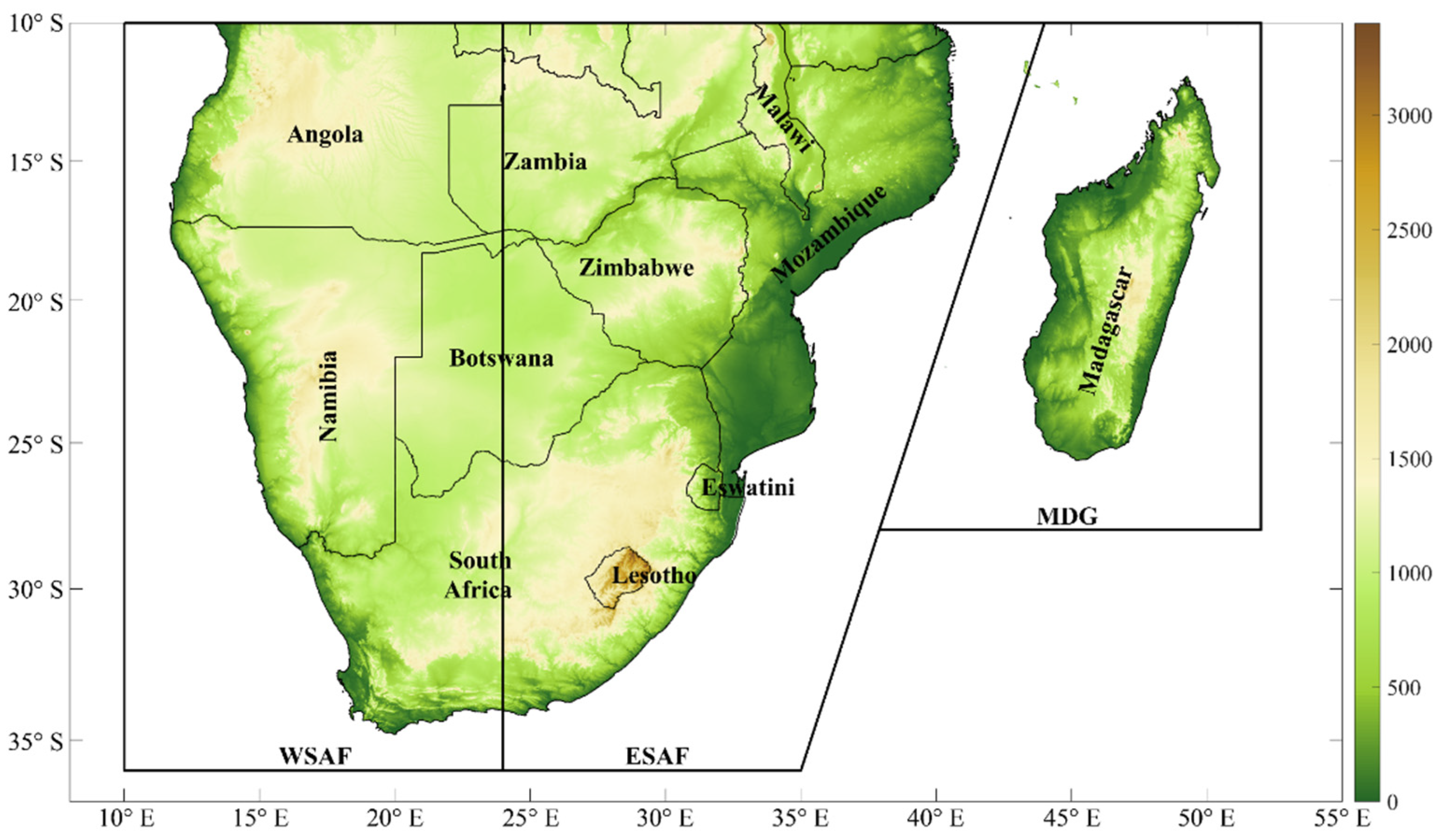
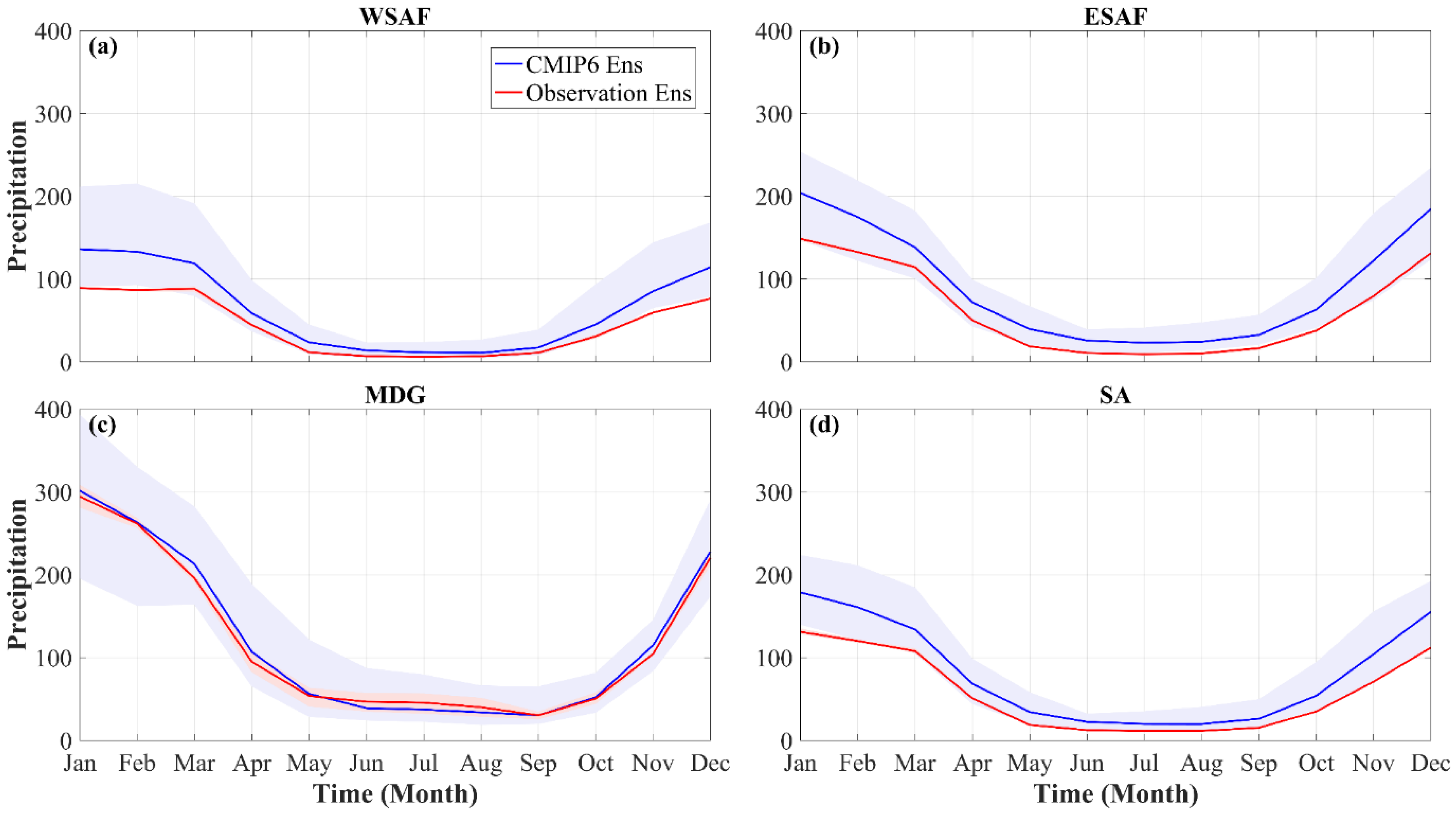
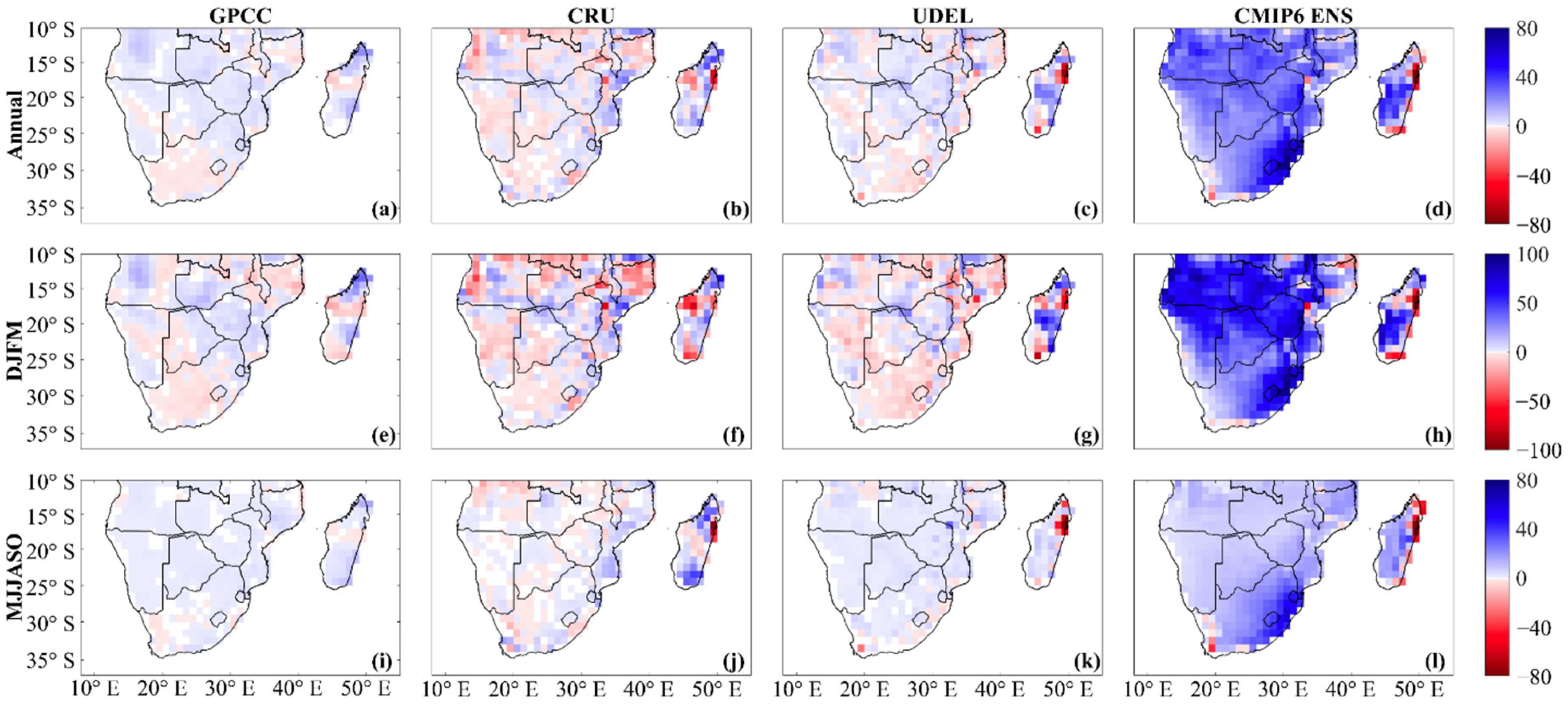
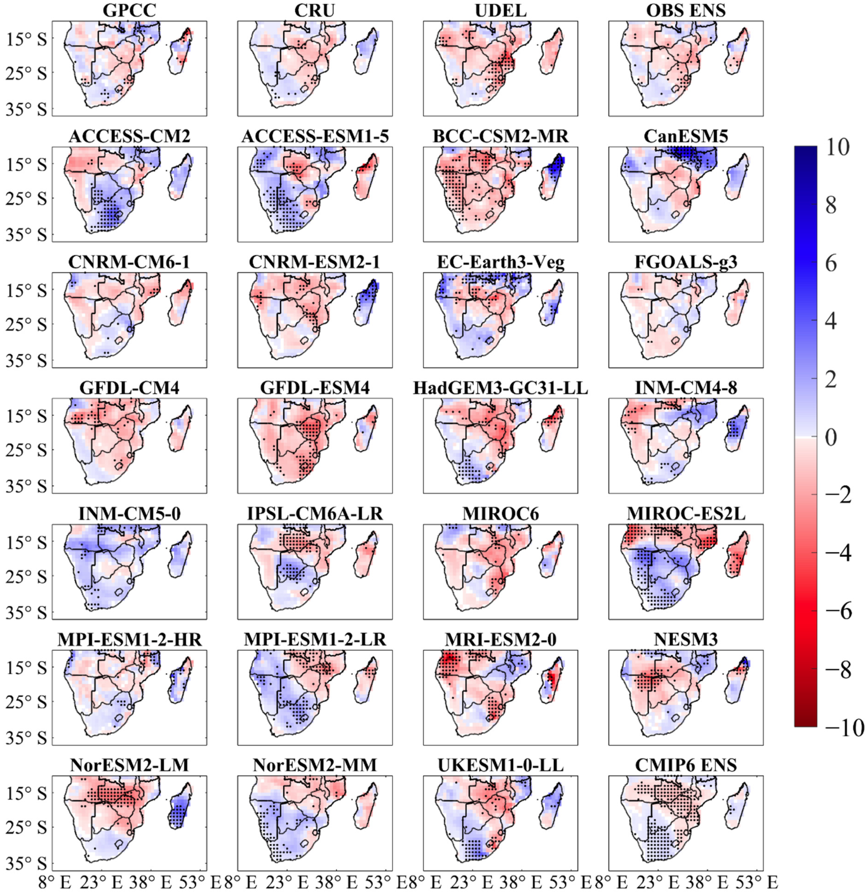
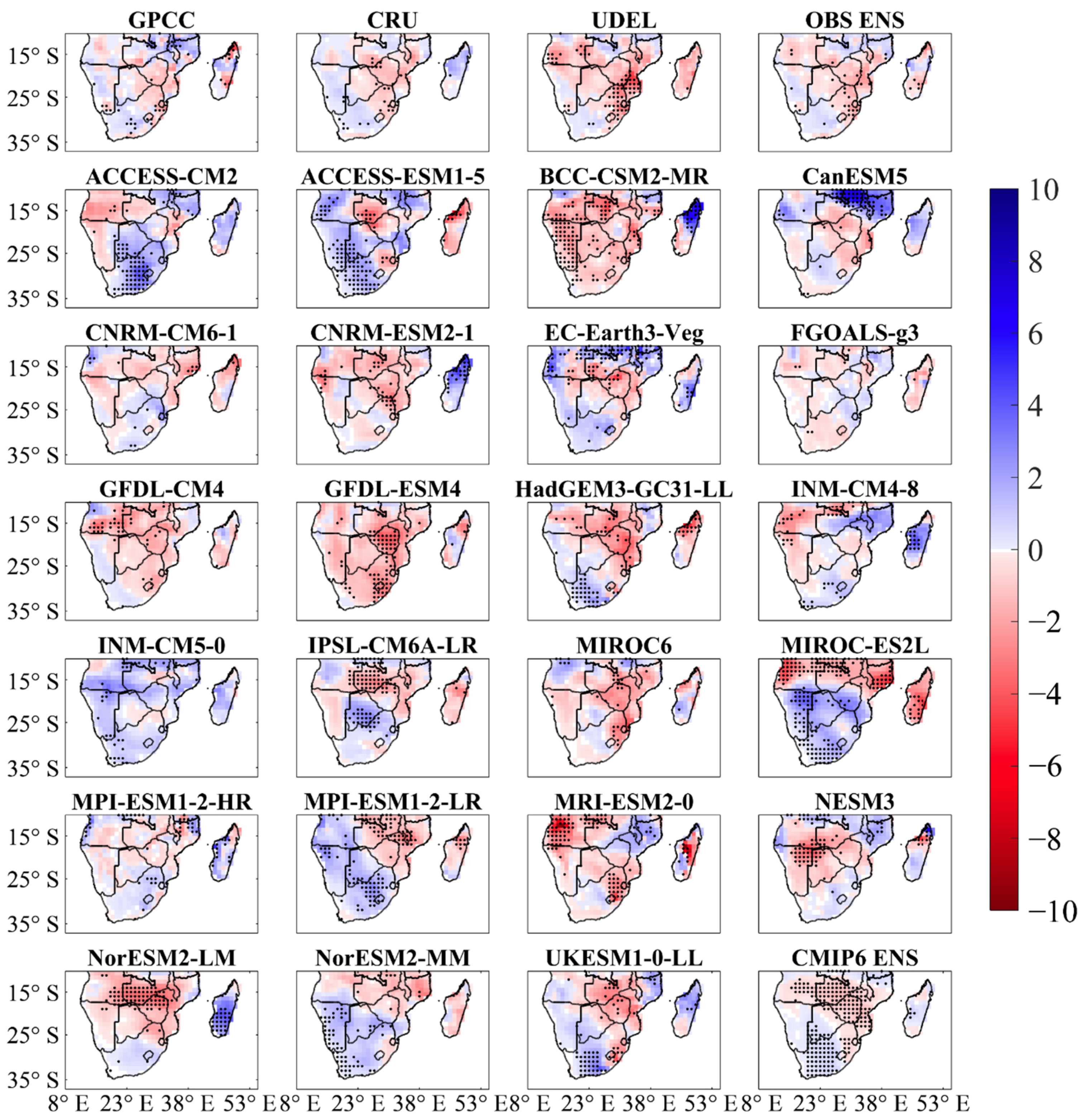
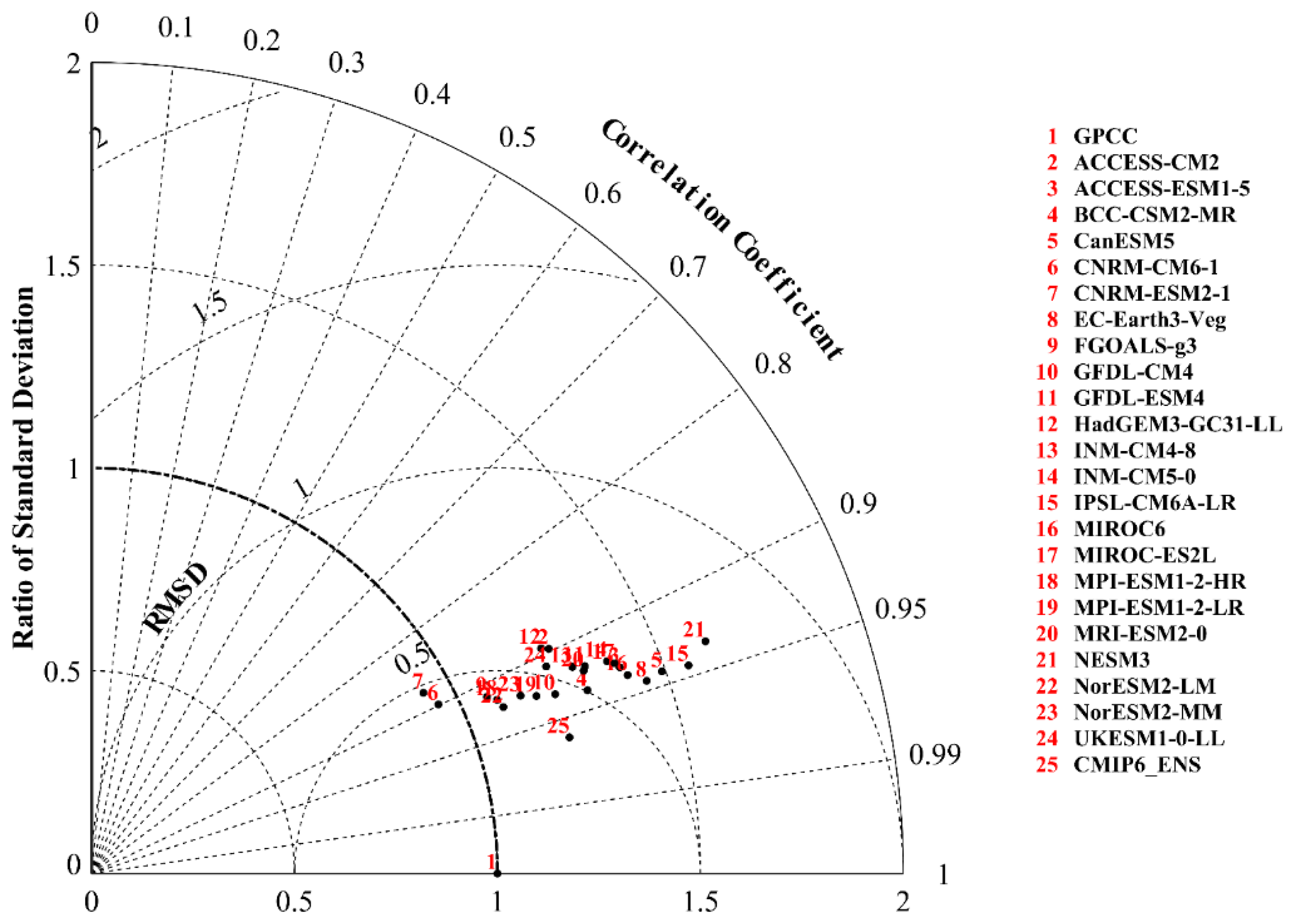
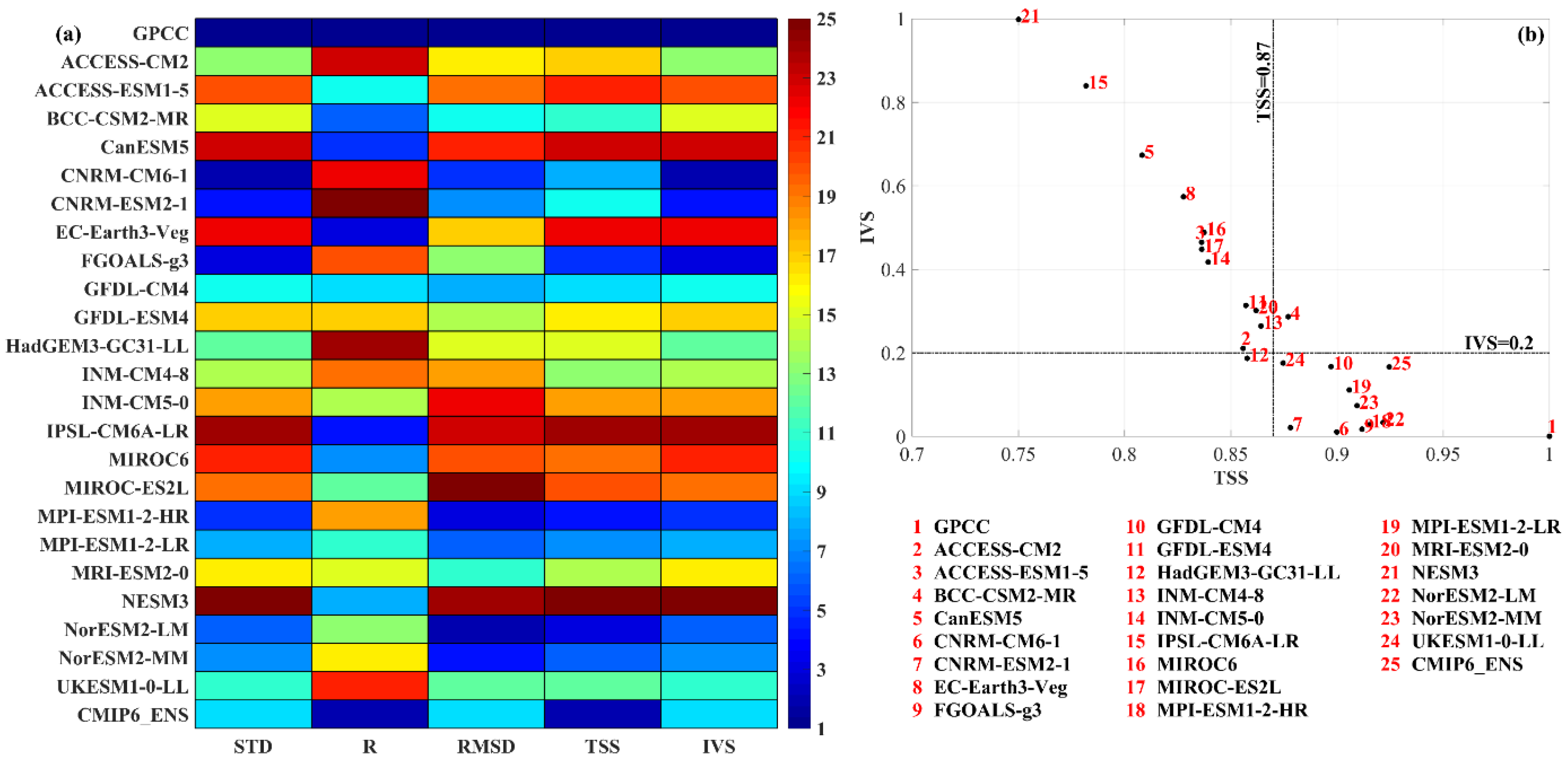
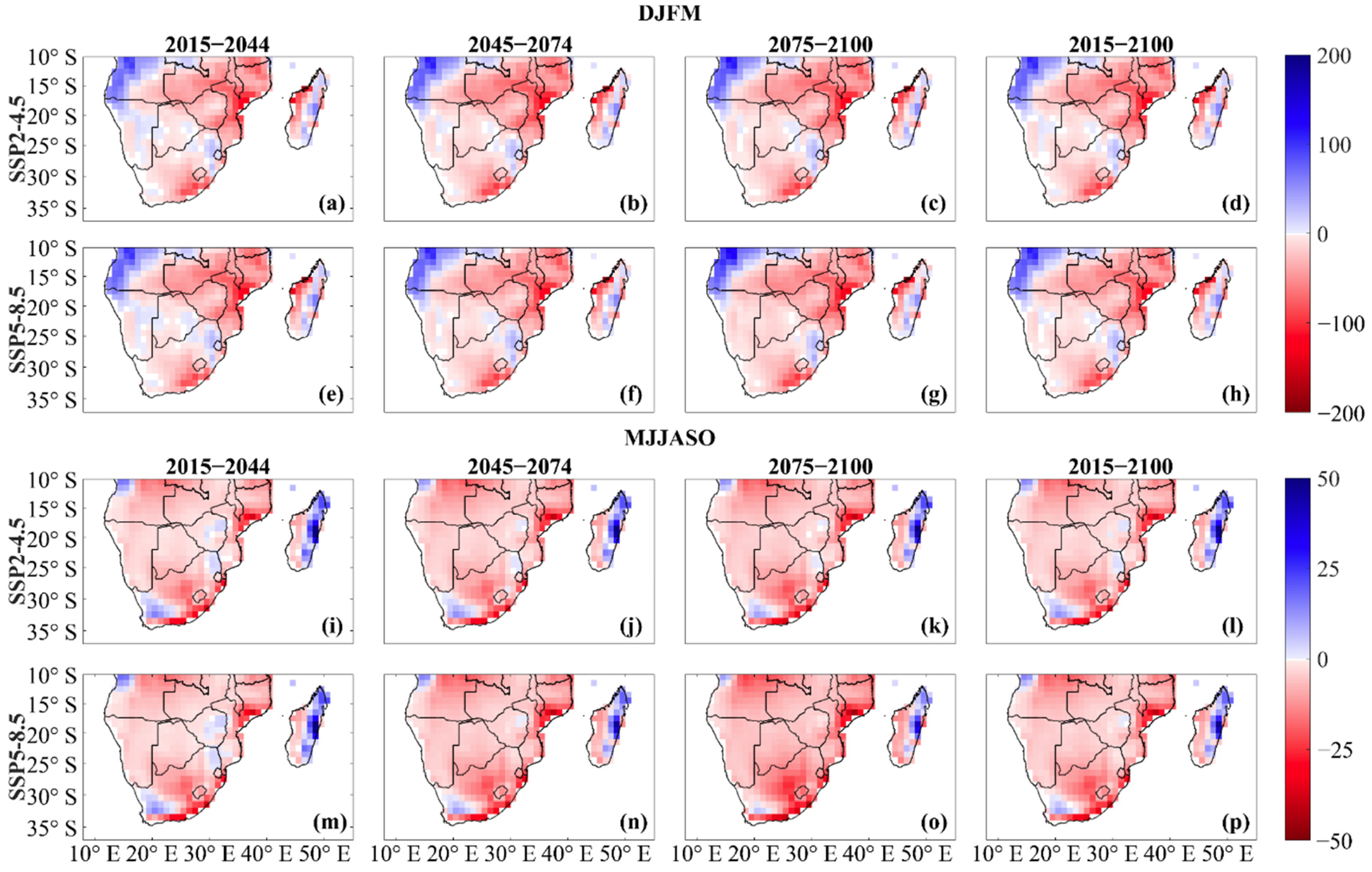
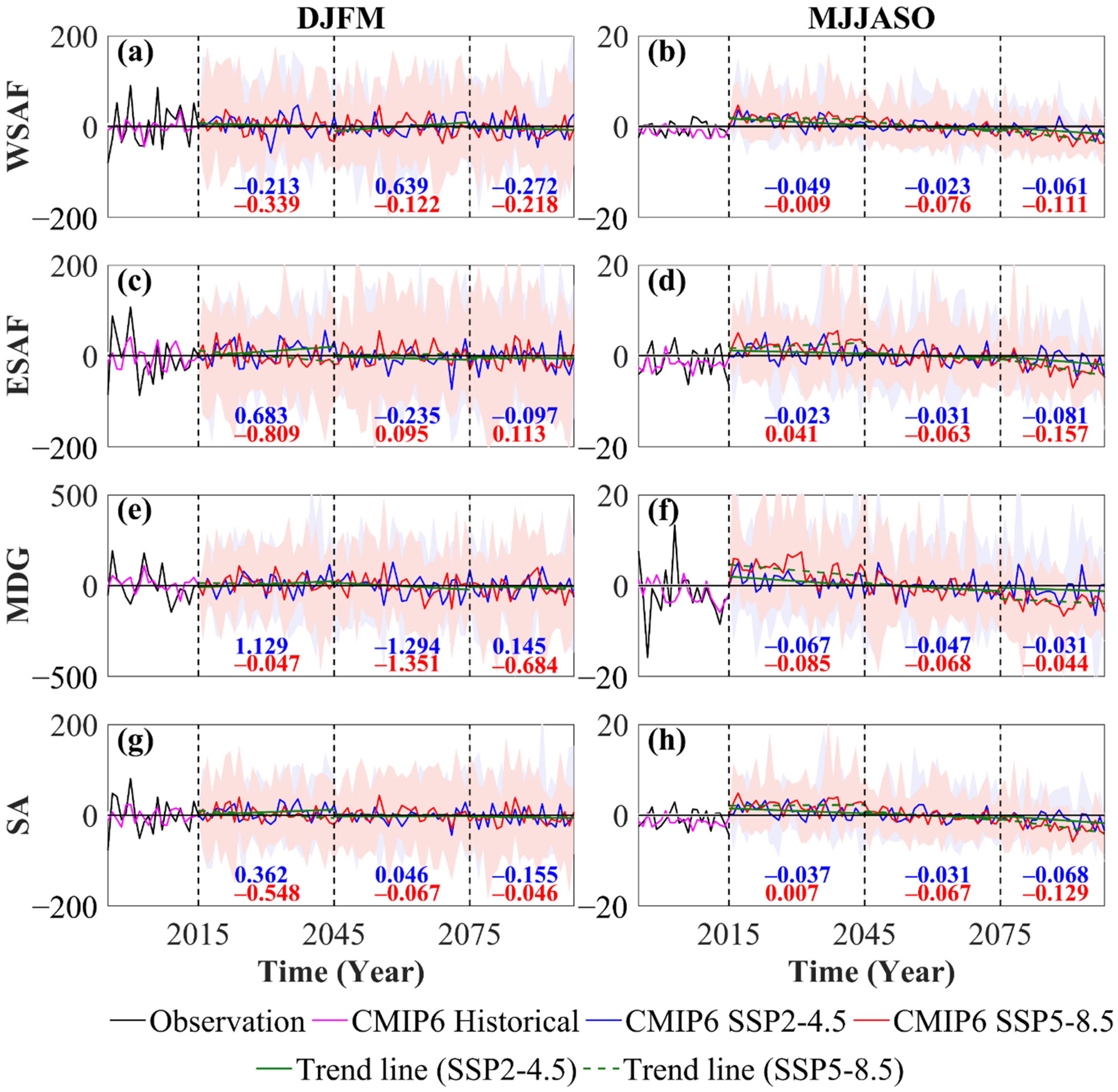
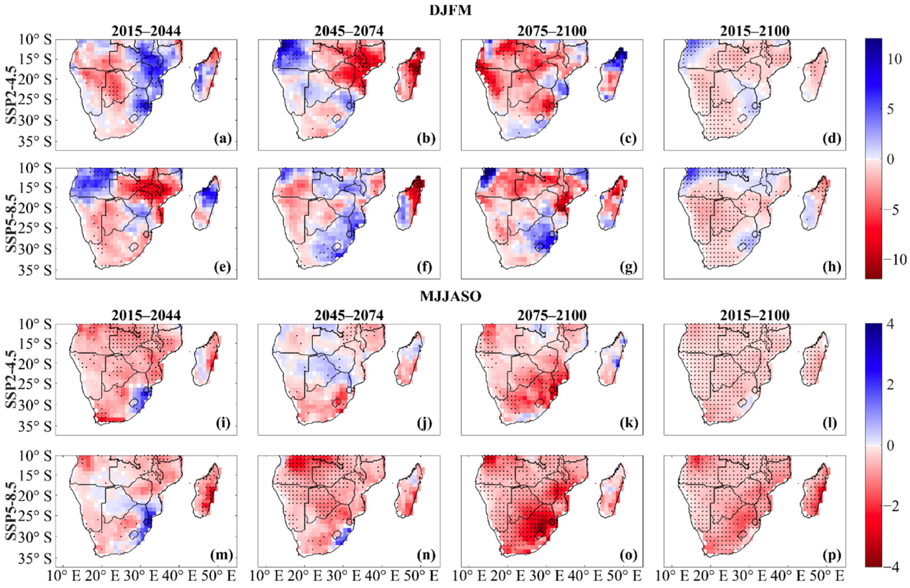
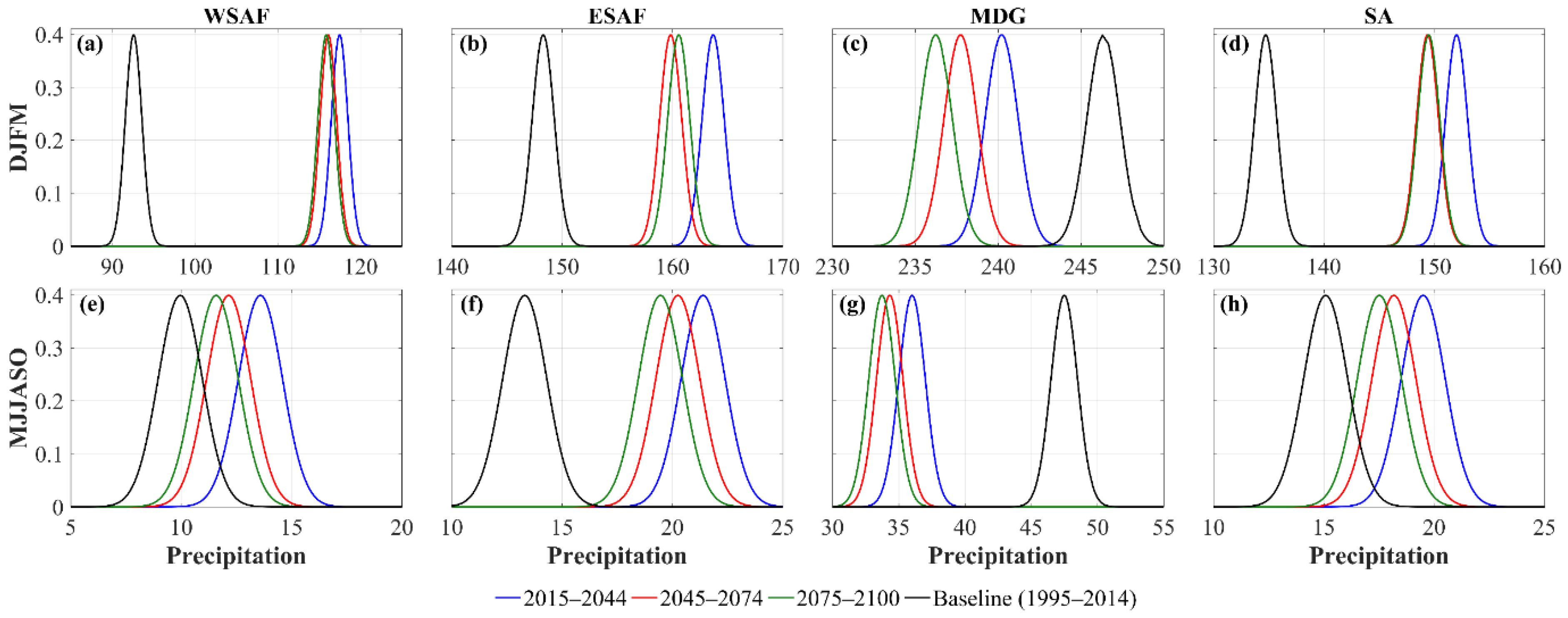
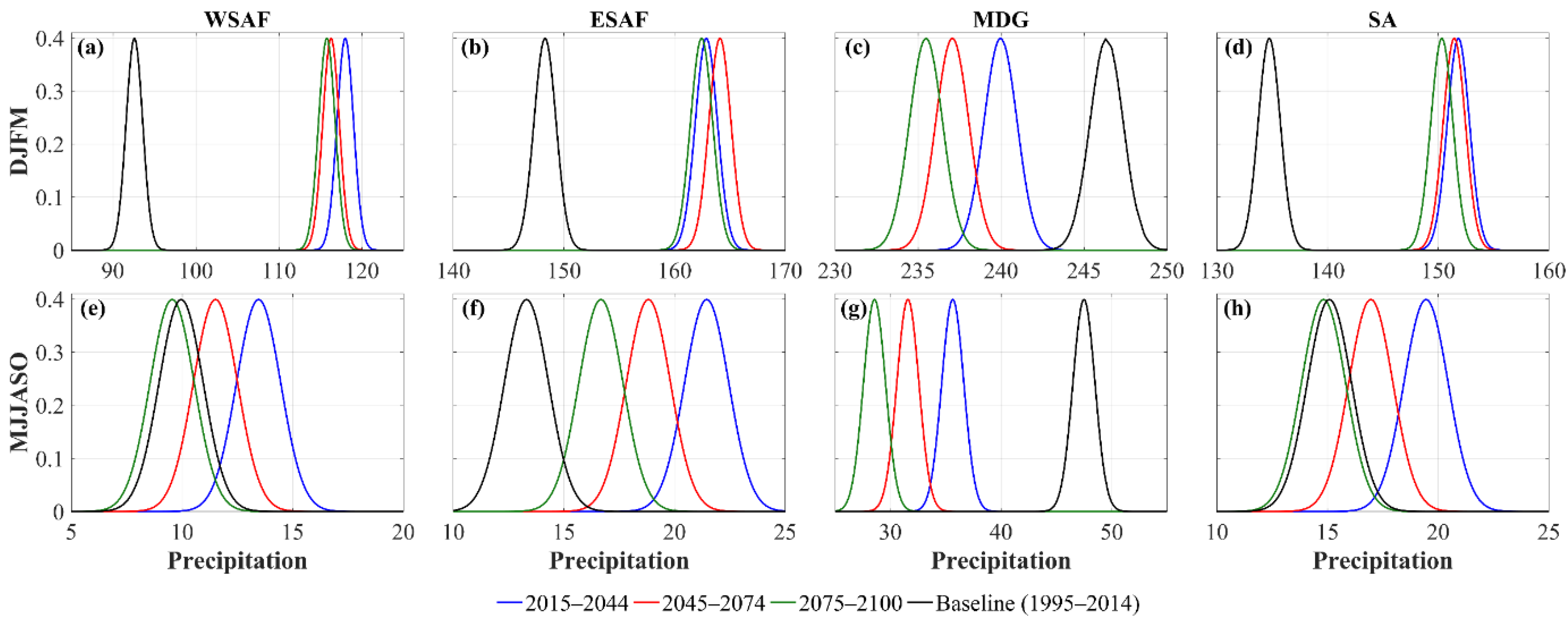
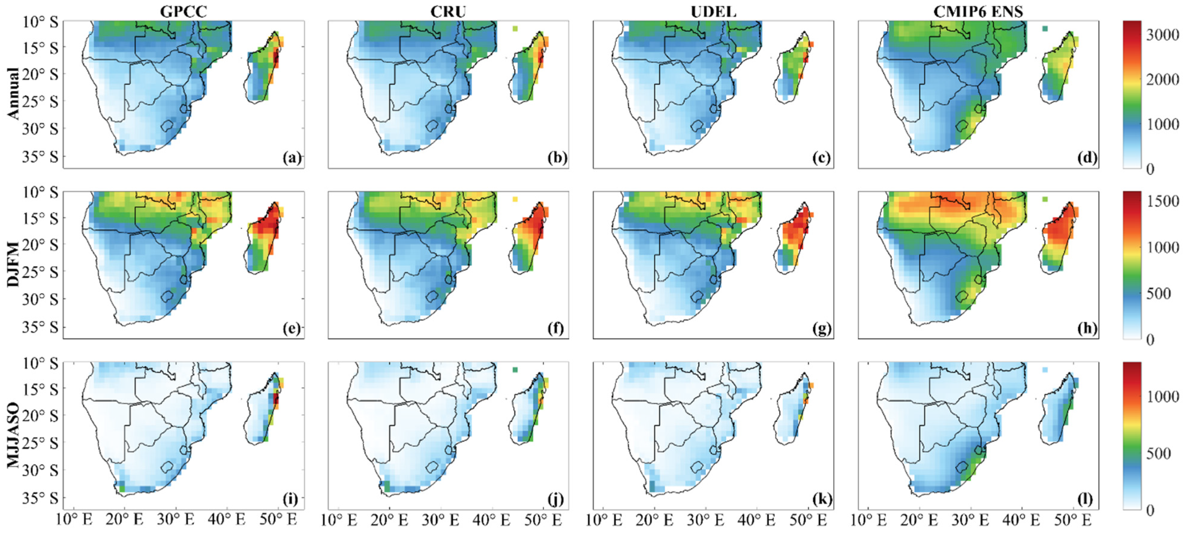
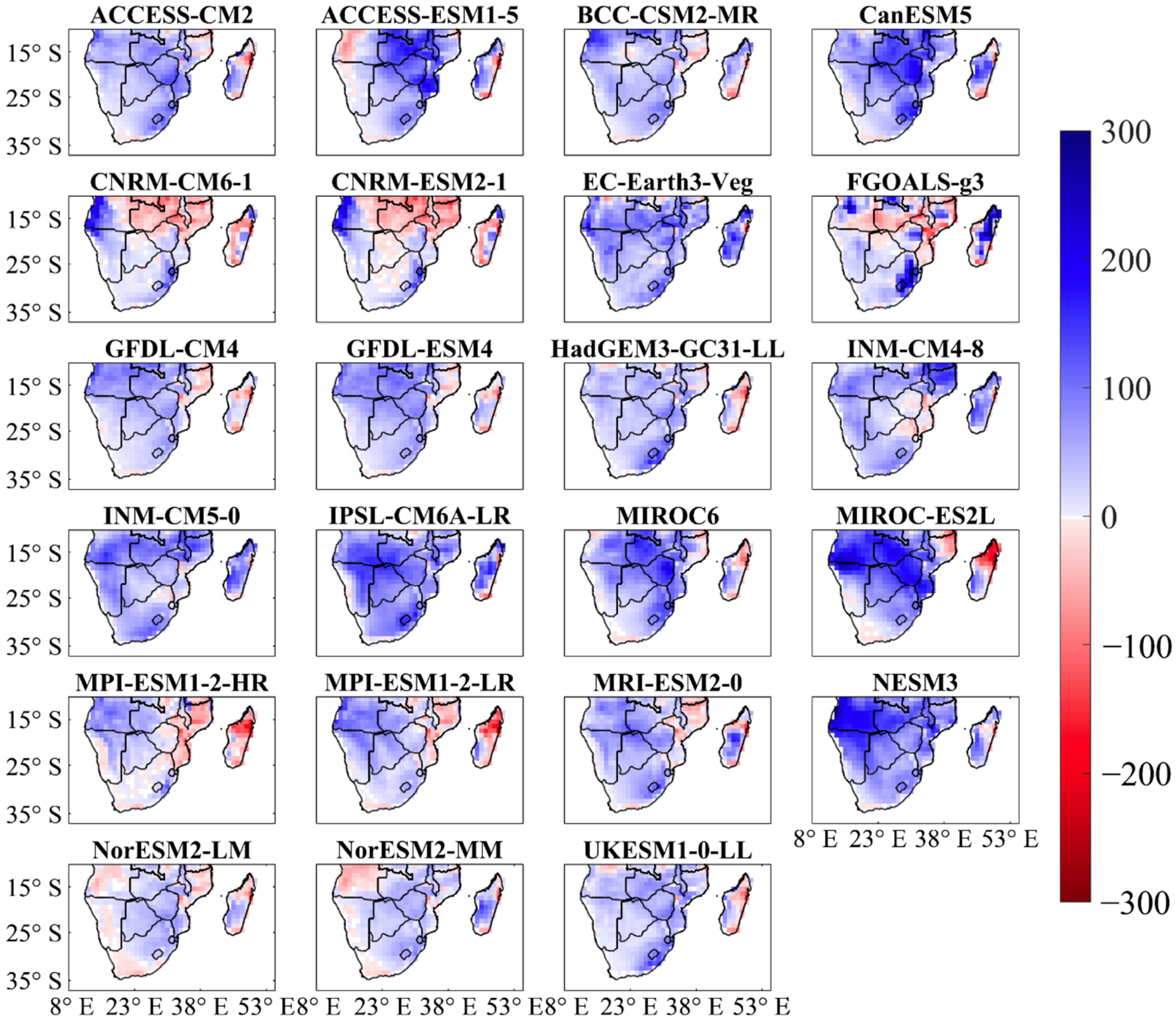
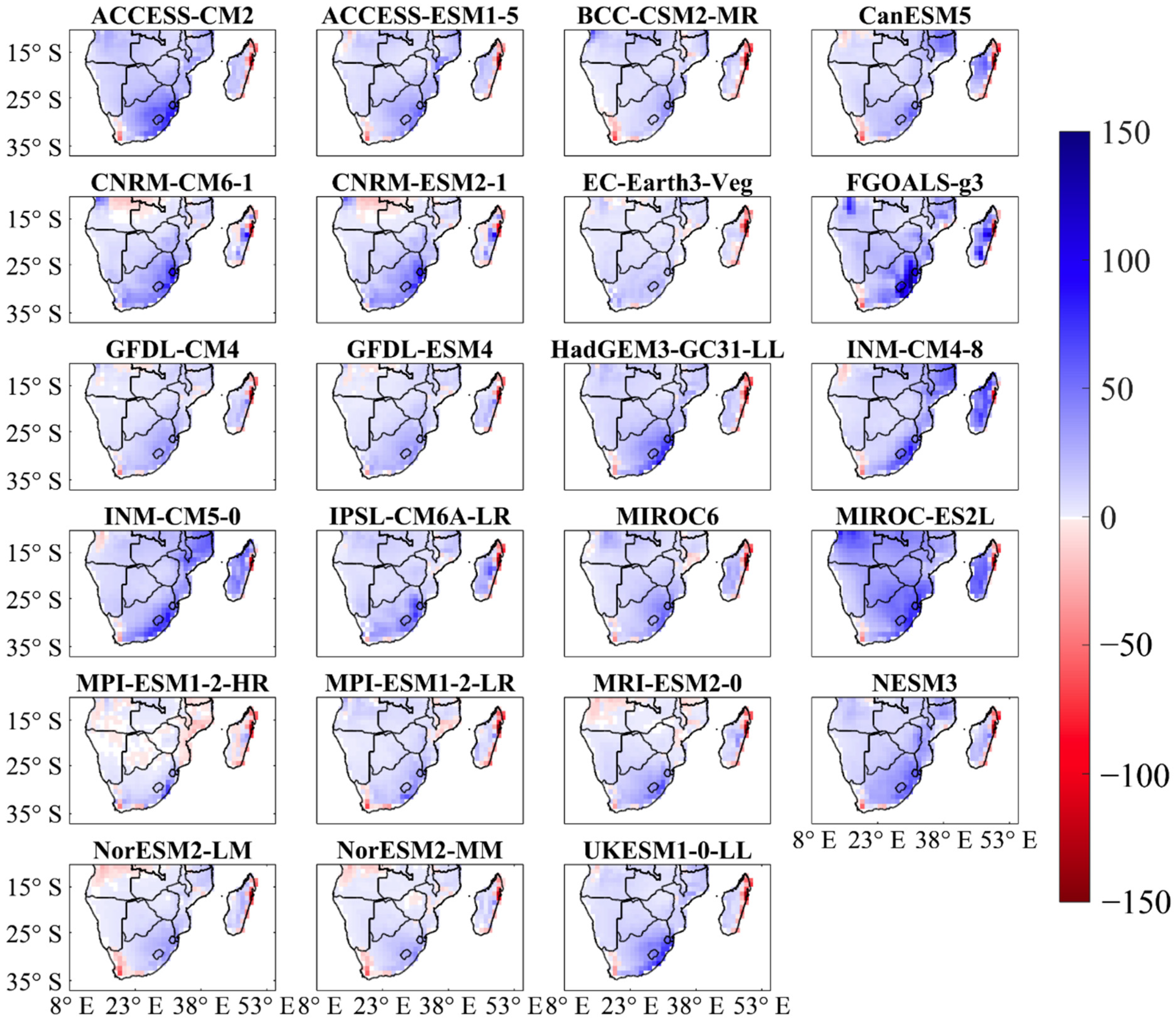
Table 1.
List of CMIP6 GCMs and their reporting institutions and countries, and grid increment horizontal resolutions.
Table 1.
List of CMIP6 GCMs and their reporting institutions and countries, and grid increment horizontal resolutions.
| Model Number | Model Name | Modeling Center/Nation | Horizontal Resolution (lat. × lon.) |
|---|---|---|---|
| 1 2 | ACCESS–CM2 ACCESS–ESM1–5 | Commonwealth Scientific and Industrial Research Organization/Australia | 1.25° × 1.875° 1.25° × 1.875° |
| 3 | BCC–CSM2–MR | Beijing Climate Center China Meteorological Administration/China | 1.125° × 1.125° |
| 4 | CanESM5 | Canadian Centre for Climate Modelling and Analysis/Canada | 2.8° × 2.8° |
| 5 6 | CNRM–CM6–1 CNRM–ESM2–1 | Centre National de Recherches Météorologiques–Centre Européen de Recherche et de Formation Avancée en Calcul Scientifique/France | 1.4° × 1.4° 1.4° × 1.4° |
| 7 | EC–Earth3–Veg | EC–EARTH consortium/Europe | 0.7° × 0.7° |
| 8 | FGOALS–g3 | Chinese Academy of Sciences/China | 2.25° × 2° |
| 9 10 | GFDL–CM4 GFDL–ESM4 | NOAA Geophysical Fluid Dynamics Laboratory/USA | 1° × 1.25° 1° × 1.25° |
| 11 | HadGEM3–GC31–LL | Met Office Hadley Centre/UK | 1.25° × 1.875° |
| 12 13 | INM–CM4–8 INM–CM5–0 | Institute for Numerical Mathematics, Russian Academy of Science/Russia | 1.5° × 2° 1.5° × 2° |
| 14 | IPSL–CM6A–LR | L’Institut Pierre–Simon Laplace/France | 1.26° × 2.5° |
| 15 16 | MIROC6 MIROC–ES2L | Japan Agency for Marine–Earth Science and Technology, Atmosphere and Ocean Research Institute, The University of Tokyo, National Institute for Environmental Studies, and RIKEN Center for Computational Science/Japan | 1.4° × 1.4° 2.8° × 2.8° |
| 17 18 | MPI–ESM–1–2–HR MPI–ESM–1–2–LR | Max Planck Institute for Meteorology/Germany | 0.9375° × 0.9375° 1.875° × 1.875° |
| 19 | MRI–ESM2–0 | Meteorological Research Institute /Japan | 1.125° × 1.125° |
| 20 | NESM3 | Nanjing University of Information Science and Technology/China | 1.875° × 1.875° |
| 21 22 | NorESM2–LM NorESM2–MM | Norwegian Climate Centre/Norway | 1.875° × 2.5° 0.9375° × 1.25° |
| 23 | UKESM1–0–LL | Met Office Hadley Centre/UK | 1.25° × 1.875° |
Publisher’s Note: MDPI stays neutral with regard to jurisdictional claims in published maps and institutional affiliations. |
© 2021 by the authors. Licensee MDPI, Basel, Switzerland. This article is an open access article distributed under the terms and conditions of the Creative Commons Attribution (CC BY) license (https://creativecommons.org/licenses/by/4.0/).
Share and Cite
MDPI and ACS Style
Lim Kam Sian, K.T.C.; Wang, J.; Ayugi, B.O.; Nooni, I.K.; Ongoma, V. Multi-Decadal Variability and Future Changes in Precipitation over Southern Africa. Atmosphere 2021, 12, 742. https://doi.org/10.3390/atmos12060742
AMA Style
Lim Kam Sian KTC, Wang J, Ayugi BO, Nooni IK, Ongoma V. Multi-Decadal Variability and Future Changes in Precipitation over Southern Africa. Atmosphere. 2021; 12(6):742. https://doi.org/10.3390/atmos12060742
Chicago/Turabian StyleLim Kam Sian, Kenny Thiam Choy, Jianhong Wang, Brian Odhiambo Ayugi, Isaac Kwesi Nooni, and Victor Ongoma. 2021. "Multi-Decadal Variability and Future Changes in Precipitation over Southern Africa" Atmosphere 12, no. 6: 742. https://doi.org/10.3390/atmos12060742
Note that from the first issue of 2016, this journal uses article numbers instead of page numbers. See further details here.