Article

Statistical Assessment and Temperature Study from the Interlaboratory Application of the WLTP–Brake Cycle

1
Joint Research Centre (JRC), European Commission, Via E Fermi 2749, 21027 Ispra, Italy
2
Link Engineering Co., 43855 Plymouth Oaks Blvd., Plymouth, MI 48170, USA
3
Ford-Werke GmbH, Henry-Ford-Straße 1, 50735 Köln, Germany
4
Audi AG, 85045 Ingolstadt, Germany
5
General Motors Company, Novi, MI 48377, USA
6
Brembo S.p.A., 24040 Stezzano (BG), Italy
7
ITT Friction Technologies, Via Crocetta 11/c, 12032 Barge (CN), Italy
8
TMD Friction Services GmbH, Schlebuscher Str. 99, 51381 Leverkusen, Germany
9
Link Europe GmbH, Am Fleckenberg 10, 65549 Limburg an der Lahn, Germany
10
Ford-Werke GmbH, Süsterfeldstraße 200, 52072 Aachen, Germany
*
Author to whom correspondence should be addressed.
Atmosphere 2020, 11(12), 1309; https://doi.org/10.3390/atmos11121309
Submission received: 4 November 2020 / Revised: 27 November 2020 / Accepted: 30 November 2020 / Published: 2 December 2020
(This article belongs to the Special Issue Study of Brake Wear Particle Emissions)

Abstract

:
The relative contribution of brake emissions to traffic-induced ambient Particulate Matter (PM) concentrations has increased over the last decade. Nowadays, vehicles’ brakes are recognised as an important source of non-exhaust emissions. Up to now, no standardised method for measuring brake particle emissions exists. For that reason, the Particle Measurement Programme (PMP) group has been working on the development of a commonly accepted method for sampling and measuring brake particle emissions. The applied braking cycle is an integral part of the overall methodology. In this article, we present the results of an interlaboratory study exploring the capacity of existing dynamometer setups to accurately execute the novel Worldwide Harmonised Light-Duty Vehicles Test Procedure (WLTP)–brake cycle. The measurements took place at eight locations in Europe and the United States. Having several dynamometers available enabled the coordination and execution of the intended exercise, to determine the sources of variability and provide recommendations for the correct application of the WLTP–brake cycle on the dyno. A systematic testing schedule was applied, followed by a thorough statistical analysis of the essential parameters according to the ISO 5725 standards series. The application of different control programmes influenced the correct replication of the cycle. Speed control turned out to be more accurate and precise than deceleration control. A crucial output of this interlaboratory study was the quantification of standard deviations for repeatability (between repeats), sample effect (between tests), laboratory effect (between facilities), and total reproducibility. Three critical aspects of the statistical analysis were: (i) The use of methods for heterogeneous materials; (ii) robust algorithms to reduce the artificial increase in variability from values with significant deviation from the normal distribution; and (iii) the reliance on the graphical representation of results for ease of understanding. Even if the study of brake emissions remained out of the scope of the current exercise, useful conclusions are drawn from the analysis of the temperature profile of the WLTP–brake cycle. Urban braking events are generally correlated to lower disc temperature. Other parameters affecting the brake temperature profile include the correct application of soak times, the temperature measurement method, the proper conditioning of incoming cooling air and the adjustment of the cooling airspeed.

1. Introduction

Non-exhaust brake particle emissions have received much attention during the last decade. There are studies reporting that the relative contribution of non-exhaust particle emissions to traffic-induced ambient PM concentrations has increased over the last decade [1]. Some mention that non-exhaust emissions have already surpassed exhaust emissions, while others project that their relative contribution to traffic-related air pollution will reach 90% by 2030 [2]. Not only the scientific community and health research organisations but also regulatory bodies and the industry around the world have been looking at the topic from different perspectives. Thus far, there is no consensus on fundamental research topics, such as real-world brake particle emission factors [3], the contribution of brake wear to ambient PM concentrations [3], and possible adverse health effects of brake debris [4,5]. However, there is a common understanding that future regulation should aim in limiting anthropogenic contributions to particulate matter from the foundation brakes.
The absence of a standardised method to measure brake emissions is partially responsible for the lack of factual data on some research topics [6]. Several different approaches for sampling and measuring brake particle emissions have been proposed. These include studies at the brake component level on a pin-on-disc configuration [7,8], at the brake couple level on a brake dynamometer [9,10,11,12,13,14,15], and at full vehicle level both in the laboratory [16,17] and on-road [18,19]. Mathissen et al. [17] summarised in detail the different setups applied for studying brake particle emissions. Despite the different approaches, there is a consensus that possible future regulation should rely on a brake dynamometer-based methodology.
Legacy duty cycles for dynamometer testing address performance, endurance, and noise test purposes (i.e., SAE J2522 for the AK Master). Recently, some of these cycles have been modified (i.e., LACT cycle) to better suit real-world applications [20], while others from the field of exhaust emissions (i.e., JC08 Transient Cycle, NEDC/WLTP) have also been employed [9,21] to study brake particle emissions. Although these cycles can provide useful information regarding brake emissions, they do not cover the full range of typical driving/braking conditions. For that reason, a dedicated Task Force (TF1) under the umbrella of the United Nations Particle Measurement Programme Informal Working Group (UNECE PMP IWG) worked on the development of a novel brake cycle which would be representative of real-world brake applications. The WLTP–brake cycle was developed and validated at the vehicle and brake-dyno level [13] and became available to the research community in 2018.
As part of developing a standard test method for sampling and measuring brake emissions, the TF1 assessed results from multiple testing facilities and research entities. The review of the findings and their value-added propositions provided evidence supporting the use of inertia dynamometer testing for studying brake emissions. Besides having the ability to follow the WLTP–brake driving profile, the dynamometer needs to feature an enclosed system with proper controls for cooling airspeed, temperature, and relative humidity (RH). Having several dynamometers available to the TF1 enabled the coordination and execution of the intended WLTP–brake cycle to determine the sources of variability at eight locations in Europe and the United States. The current paper aims to present a high-level statistical assessment, as well as some first findings regarding the implementation of the WLTP–brake cycle to different brake dynamometer facilities. The study of brake emissions remained out of the scope of the current exercise.

2. Experiments and Methods

2.1. Inertia Dynamometer Capabilities

Labs conducted all measurements using single-ended performance or single-ended Noise, Vibration and Harshness (NVH) dynamometer with standard data collection and control systems. Lab 8 employed a performance dynamometer adapted for emission measurements; however, did not conduct any emissions measurement within the current study. Regarding climatic controls, several labs featured full climate control of the inertia dynamometer at (20 ± 2) °C and (50 ± 5)%RH. All labs were requested to use dynamometers capable of regulating incoming cooling airflow rate to replicate the vehicle’s brake temperature profiles. The labs were requested to run the dedicated control programme provided by Ford Werke GmbH (Ford) or by Link Engineering Co. (LINK); however, the application of lab-specific internal control programmes was acceptable. All labs employed rigid fixtures without a dust shield built from a vehicle knuckle assembly. Table 1 summarises the hardware and testing conditions applied to the interlab comparison.
The main objective related to the incoming cooling airflow is to adjust it to the vehicle’s temperature regimes. The baseline thermal regimes were derived from the proving ground measurement conducted during the development phase of the WLTP–brake cycle. The base proposal for adjusting the dynamometer cooling airspeed (or airflow) used the best fit curve for the cooling phase of two high‒speed events of Trip #10 of the WLTP–brake cycle. Alternatively, labs were allowed to adjust the cooling settings to achieve the best fit with vehicle temperature applying the full duration of Trip #10. The preferred mounting position for the calliper was to mimic the in-vehicle position relative to incoming cooling air.
Another critical parameter to consider—within each dynamometer’s capabilities—is the parasitic vehicle losses. No standard method for correcting for the parasitic losses was available at the time of the exercise. Therefore, each lab applied their respective control software to reduce the total torque demand from the foundation brake to reflect the vehicle’s resistive forces. The correction of the torque set-point improved the braking behaviour’s fidelity compared to the vehicle, the dissipation of kinetic energy, and the thermal regimes on the dynamometer.

2.2. Brake Components

All labs received three sets of production discs and brake pads. Two of the sets were from the same batch used for the vehicle measurements on the proving ground [13]. More specifically, Ford Werke GmbH distributed among the labs two grey cast iron brake discs and two pairs (inner and outer) of low-metallic brake pads typical of the European market. The third (spare) set was of similar specifications and allowed the verification of the test setup, cooling air adjustment, and fine-tuning of the control programmes.
Each lab used in-house fixtures using OEM‒level brake L1 knuckle assemblies. The labs received production callipers from the same batch. The labs used a threshold pressure of zero and a calliper efficiency of 100% to calculate the coefficient of friction. Mathissen et al. [13] provide additional details regarding the brake components used in the current exercise.

2.3. Test Cycle and Application of Control Program

The testing schedule selected for this interlab exercise was the WLTP–brake cycle. The cycle was developed based on real-world driving data derived from the WLTP reference database. It consists of 303 braking events split into 10 consecutive trips (Trip #1–Trip #10) with a total duration of approximately 4½ h plus the soak periods in-between trips. The cycle includes distinct segments for urban, rural, and motorway driving. The cycle itself and the methodology followed for its development are described in detail by Mathissen et al. [13]. Additional metrics for speed, deceleration, kinetic energy, and brake power dissipation, along with a list of brake events, are available in the PMP Brake Emissions Protocol—Part 1 [22].
All labs were requested to follow the WLTP–brake cycle by applying the time-resolved speed trace. As described previously, and reflecting the nature of the laboratory testing, dynamometers (vintage and capabilities) and control programmes were different in several cases. As a result, the different control strategies induced differences in some of the labs’ primary input parameters with visible effects on the outcomes. Other variability sources include the servo controller’s specific response, the brake application system, and the actual algorithm to correct (compensate) for parasitic vehicle losses.

2.4. Test Schedule at Each Lab

The study involved eight labs from Europe and the United States. Labs agreed to conduct two tests (T1 and T2), with each test comprising six repetitions (R1 to R6) of the WLTP–brake cycle, which itself consists of 10 trips (Trip #1 to Trip #10). T1 was performed with new brake components. T2 used the same brake couple as in T1. Not all labs managed to follow all requirements and suggestions, due to technical limitations or time constraints (Table 1). Figure 1 illustrates the simplified structure of the tests. Within each repetition, after the end of each trip and before initiating the next trip, the sequence includes a soak time to allow the disc temperature to cool down and reach 25 °C.
During the cooldown, the dynamometer imposes a slow rotation of the disc. The setup used an embedded thermocouple (hereafter mentioned as TCEmb) in the disc’s friction area. The TCEmb measured the brake temperature in real-time and controlled the start of each trip. The location of the TCEmb was in the braking surface of the outboard plate (wheel side). The TC’s radial position was 10 mm outwards from the centre of the friction path and recessed 0.5 mm below the braking surface [22]. Besides, some labs installed a rubbing TC (hereafter mentioned as TCRub) with the radial position as the TCEmb. Besides the TC(s) mounted on the disc, the labs embedded one additional TCEmb to measure the brake pad’s temperature, located in the outer pad’s centre, 1 mm below the braking surface.

2.5. Overview of Outputs and Test Results

Labs agreed to report test outputs using the standard format VDA 305/EKB 3008 [23]. After the testing campaign, each lab submitted the EEC and EED files for T1 and T2.
The EED files’ adaptation to the WLTP–brake cycle creates a single file for the entire cycle for each repeat. Essentially, an EED file is a table, of which each column represents a measurement signal. Every row on the EED file represents a sampling period. The main parameters reported as time-resolved values at 1 Hz for each test (T1-T2), each repetition (R1-R6), and each trip (#1-10) included: Elapsed time [s]; Brake linear speed [km/h]; Brake deceleration [m/s2]; Brake torque [N·m]; Brake pressure [bar]; Friction coefficient μ [‒]; Disc and pad temperatures [°C]; Cooling airspeed [km/h]; Cooling air temperature [°C]; Cooling air RH [%].
The EEC file is the primary data exchange format as a CSV file. This type of file makes the data exchange among testing facilities independent to the original software used on a given dynamometer. The main parameters reported as time-resolved values at 1 Hz for each test (T1-T2), each repetition (R1-R6), and each trip (#1-10) included: Trip [#]; Time and date of the braking event [–]; Initial braking speed set-point and actual [km/h]; Final braking speed (release speed) set-point and actual [km/h]; Deceleration set-point and actual [m/s2]; Average-by-distance brake torque [N·m]; Average-by-distance brake pressure [bar]; Average-by-distance friction coefficient μ [‒]; Initial, final, and maximum disc temperature (TCEmb and TCRub) [°C]; Initial, final, and maximum brake pad(s) temperature (TCEmb) [°C]; Average-by-time cooling airspeed [km/h]; Average-by-time cooling air temperature [°C]; Average-by-time cooling air RH [%].

3. Results and Discussion

3.1. Statistical Evaluations

3.1.1. High-Level Statistical Evaluation for Braking Speed and Total Deceleration

The first level of statistical assessment focuses on answering two critical questions—how accurate were the different labs to control the brake speed and the deceleration from the WLTP–brake cycle? Kinetic energy is a function of the square of the braking and release speeds; therefore, the study of braking speed provides an insight into the primary input to the amount of kinetic energy dissipated by the brake. Additionally, assessing brake deceleration provides useful metrics related to the rate of kinetic energy dissipation (braking power), and thus, brake temperature rise during braking. Table 2 presents the essential speed, and deceleration statistics for all labs averaged over the six repetitions of T1. Table 2 also provides a high-level summary of the corresponding vehicle statistics (WLTP). The summary metrics depict the behaviour for the entire cycle and its urban, rural, and motorway sections.
This part of the statistical evaluation involves all events and is separated by type of driving (urban, rural, motorway) as defined in Valverde et al. [24]. All the estimates (in absolute values or as a per cent) for accuracy/bias and precision/scatter relate to the nominal value established on the WLTP–brake cycle. Accuracy of braking speed and deceleration is the bias or deviation from its nominal value. The braking speed and deceleration precision measured as scatter or variability corresponding to a 95% confidence interval from the six repeats of the cycle during T1. The data review for most labs shows that the application of different control programmes influenced the correct replication of the cycle. The root causes for such discrepancies may relate to programming errors, the dynamometer control programme skipping or missing certain brake events, and data entry errors during the compilation of results from all labs. The WLTP–brake cycle has many brake events combined with drastic differences in set-points between consecutive events. This makes the metrics for test quality highly sensitive to potential errors in the control programme, data collection, or data reporting. Since there is no intention to migrate towards a unique and universal control programme, it is necessary to ensure all labs conducting this cycle rely on standard speed metrics and an agreed-upon method to correct for parasitic vehicle losses.
Overall, speed control seems to be more accurate and precise than deceleration control. Most dynamometers convert the deceleration set-point to an equivalent torque set-point. The relatively low torque levels during the WLTP–brake cycle on the primary test vehicle (from 160 N·m to 200 N·m on average on the front axle’s brake) can coalesce with other mechanical, electrical, and servo response characteristics (hysteresis, linearity, accuracy, zero offsets, ramp rates, and hydraulic servo‒controller settings, among others). For the vehicle under test, the average braking torque equates to less than 5% of a typical inertia dynamometer’s full scale.
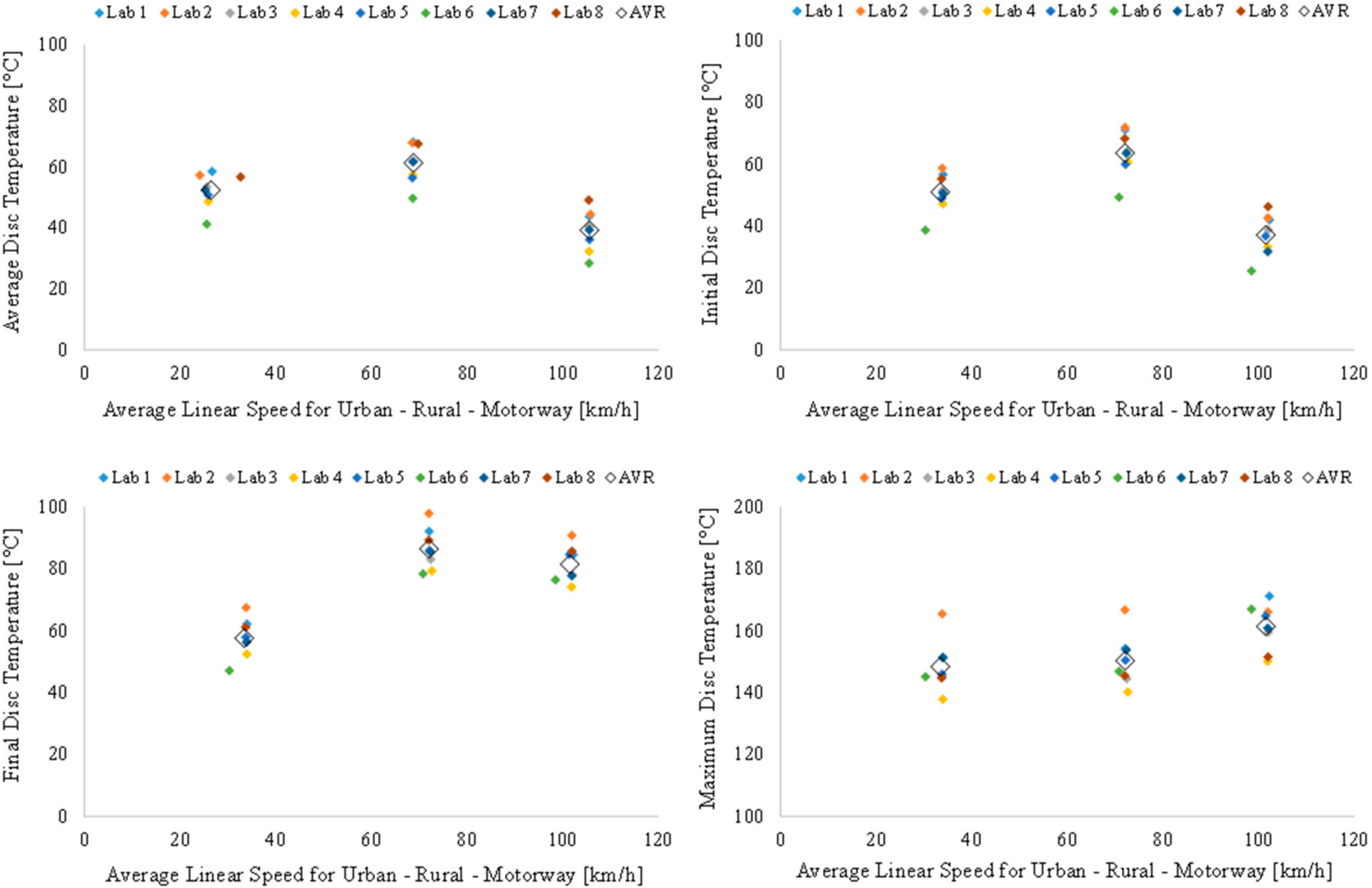
Accuracy/bias for each lab and speed range relative to the nominal set-points from the WLTP–brake cycle displayed as a scatter plot in Figure 2 (left-hand side). The bias in speed is smaller than 1 km/h compared to the individual set-points; the weighted bias compared to the nominal WLTP–brake cycle is 2.1 km/h (4.6%) on average for all labs combined. Labs 3, 4, 7, and 8 exhibited a weighted average bias below 0.2 km/h (1%). Lab 5 exhibited a bias comparable to the overall averages except for an average bias of 20 km/h during the motorway section. Labs 1 and 2 exhibited a weighted average between 4–5 km/h, with rural and motorway events being more penalised. Lab 6 exhibited a systematic bias or about 4.5 km/h (>10%) for all types of brake events. Regarding deceleration, labs exhibited a weighted average bias of 0.13 m/s2, which corresponds to 13% of the nominal value. It is noteworthy that Labs 1, 4, and 7 controlled the brake with a bias higher than 15%. These labs indicated issues with the design of the control programme and the use of an incorrect set of parameters for the parasitic vehicle losses. Labs 3 and 8 exhibited the smallest bias in all three different speed ranges.
Precision/scatter for each lab and speed range relative to the nominal set-points from the WLTP–brake cycle displayed as a scatter plot in Figure 2 (right-hand side). On average, all labs exhibited a speed variation lower than 0.5% during 95% of the brake events for all six repetitions of T1. Labs 1, 4, and 8 had the smallest scatter (less than 0.2%), while Labs 3, 5, and 6 exhibited a weighted average scatter close to 1%. As expected, urban brake events exhibit the most significant level of variability compared to rural and motorway events. Regarding deceleration, data from all labs show that the weighted average scatter is 3.3% of the nominal deceleration levels. This value is below the legacy limit of 5% accepted for torque control. The tolerance for torque control combines actual deceleration rate and brake inertia. Labs 1, 4, 7, and 8 were able to limit variability to 1.5% on average, while Labs 2 and 5 exhibited variability of about 8.5% (mainly due to urban braking events). The scatters for all rural and motorway events for all labs remained low as they did not exceed 1.8% of the nominal. Another source of variability is the variance in the reference deceleration measured on the vehicle at the proving ground. Using data from proving ground on different vehicles, the variance on deceleration is estimated at 8.85 × 10⁻⁵ (m/s2)2 [25].
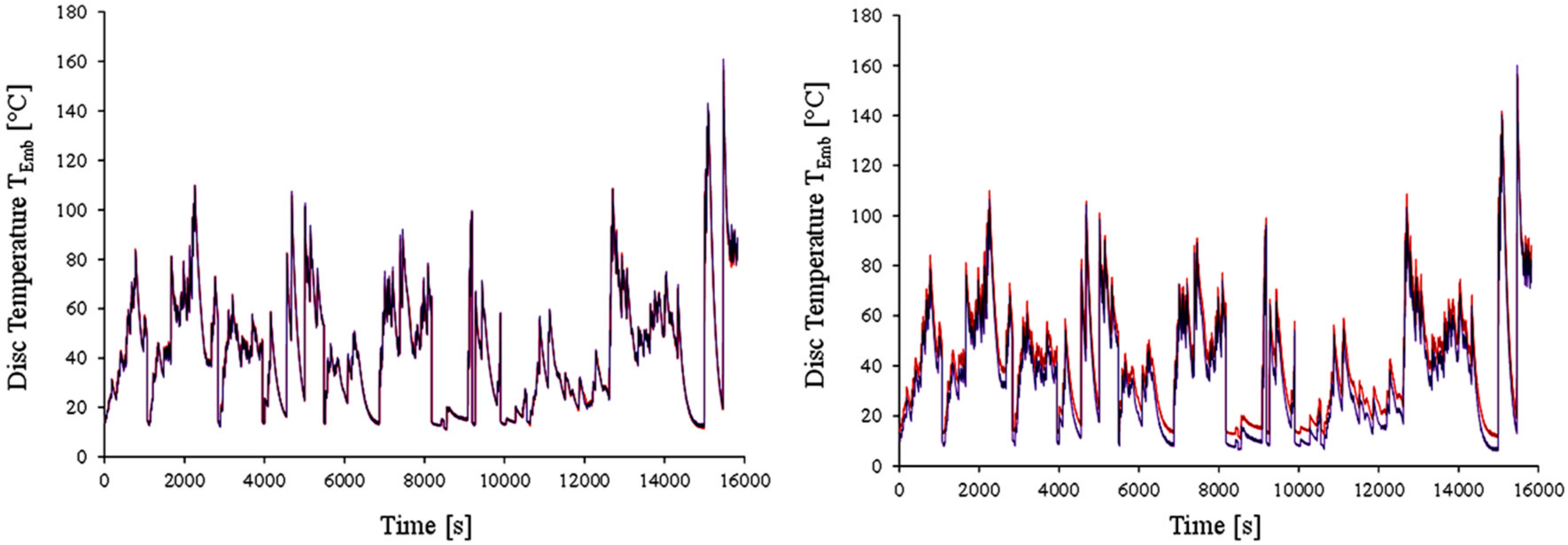
Regarding deceleration, the application of different control programmes and test parameters can influence the correct replication of the brake power dissipation during the cycle. For example, Figure 3 illustrates the distribution of all braking events (T1–R1) for Labs 1 and 3 based on deceleration rate bins of 0.1 m/s2. As discussed previously, Lab 1 executed significantly more braking events with a deceleration higher than 1.0 m/s2 compared to Lab 3 and the nominal WLTP–brake cycle. As a result, the average deceleration rate for Lab 1 over the entire cycle is higher.
These findings indicate that some labs might need to revise their control strategy to improve the precision—mainly, but not only, during urban events. These events comprise almost 85% of the brake events during the WLTP–brake cycle; therefore, they are the most significant part of the overall cycle.
Figure 4 shows the linear relationship of braking deceleration between each lab and the vehicle. Even though most labs exhibited high linearity (high R‒squared factor), the linear relationship to vehicle level (slope factor) varied from 0.8143 for Lab 7 to 1.4274 for Lab 1. Labs 1 and 4 exhibited significantly higher deceleration above the nominal. On the other hand, Labs 6 and 7 indicate significantly lower deceleration below the nominal, with Lab 6 showing more significant bias at decelerations below 1 m/s2. The regression for Lab 6 uses a total least squared regression to include the variance on vehicle deceleration per the method and the spreadsheet illustrated by Cantrell et al. [26]. Comparing the common linear least squared regression (minimising the vertical distance to the regression line) to the total least squared regression (minimising the perpendicular distance to the regression line) for other labs yields a difference of less than 1%. The values in Figure 4 reflect the deceleration levels for the foundation brake after correcting for the resistive vehicle forces. The differences in brake deceleration levels also help explain some of the variations observed in brake temperatures discussed later in the document.

3.1.2. Statistical Assessment of Time-Resolved Speed Violations and Error

The next level of numerical assessment of the dynamometer data pertains to the time-resolved speed response at 1 Hz. The two standard metrics to qualify the cycle’s execution relative to the speed trace include: (i) Speed violations as the % of the time the brake speed were outside the limits established on the Annex 6 of the UN GTR No. 15–5th amendment (6th amendment to be published soon) [27]; and (ii) Speed error as the Root Mean Square of the Speed Error (RMSSE) per SAE J2951 [28] also expressed as % of the maximum error allowed by the GTR 15. The cited documents provide more details regarding the implementation of the metrics.
This paragraph aims to determine for every nominal value on the speed trace at 1 Hz whether there is a speed violation or not. According to Annex 6 of the UN GTR No. 15, the speed trace for a given timestamp t is allowed to deviate from the nominal value within a predefined threshold of ±2 km/h. When the speed trace exceeds this threshold, then a violation is recorded for the given timestamp t. The calculation for total speed violations (above and below) for the entire trip follows Equation (1). More details regarding the equations and the metrics’ implementation can be found to the respective Global Technical Regulation and its recent amendment [27].
S v i o l ,   % = t = 1 15826 a b s ( S v i o l , t ) 15826
In Equation (1) S v i o l ,   % represents the total speed violations, as a per cent of the entire drive-on time of the WLTP–brake cycle (15,826 s), and a b s ( S v i o l , t ) is the count of instances (at 1 Hz) when the dynamometer speed is below or above the speed tolerance. Table 3 indicates the summary of speed violations as a per cent of total time for all six repetitions of the WLTP–brake cycle on T1. Lab 6 did not exhibit any speed violation, followed closely by Labs 4 and 5, which performed the cycles with less than 3% of the time being outside the nominal speed profile. On the other hand, Labs 3 and 8 exhibited 42% and 32% of speed violations, respectively, failing to correctly follow the nominal speed profile. Labs 1 and 2 exhibited more significant numbers of speed violations during R1, whereas significantly improved to the following repetitions. This behaviour hints to possible control programme optimisations before continuing to subsequent repetitions. In contrast, Lab 8 performed the first five repeats with ~37% speed violations and made changes to R6 to reduce the violations to 0.5%.
The examination of the RMSSE parameter yields similar conclusions. For each timestamp of a given speed trace, the RMSSE for a given cycle as a per cent is determined using Equation (2). More details regarding the equations and the metrics’ implementation are available at the Society of Automotive Engineers (SAE) Standard J:2951 [28].
R M S S E %   = R M S S E R M S S E l i m i t × 100 %
RMSSE% is the ratio between the RMSSE of the entire test and the RMSSElimit calculated for the upper or lower speed limits defined per GTR 15 or GRPE 81-12, expressed as a per cent. Table 4 indicates the summary RMSSE (km/h) and per cent RMSSE for all repeats on T1. The WLTP row refers to the maximum RMSSE metric while still complying with the speed tolerance. Labs 4 and 6 managed to conduct the six repeats below 50% of the acceptable limit, while Lab 5 did not exceed the acceptable limit in any of the repeats. Labs 1 and 2 completed five repeats between 85% and 95% of the acceptable limit. Labs 7 and 8 had only one or two repeats below the maximum RMSSE limit of 3.2 km/h (rounded value for 3.191 km/h).
It is essential to contrast the speed metrics (using the entire 1 Hz dataset) with the accuracy and precision during braking to understand the speed control during the cycle fully. Even though Labs 3, 7, and 8 exhibited a performance comparable or better than other labs in the latter metrics (braking speed and average deceleration), the two metrics for speed (speed violations and RMSSE) for the entire cycle (at 1 Hz) tended to exhibit lower-than-average performance. It is interesting to note that Lab 3 develops braking decelerations with high‒fidelity compared to the WLTP–brake cycle. This contrast hints that Lab 3 performed better during braking than in-between braking events (Table 2).

3.1.3. Statistical Analysis and Derivation of Standard Deviations Per ISO 5725-5

The analysis provided in this part relies entirely on the series of ISO 5725-5 standards. The current study followed the general guidance designed for heterogeneous materials [29], while the general formulae accommodate the fact that not all labs were able to report all the results for each level-braking event [30]. The general statistical approach involves three factors arranged in a specific hierarchy: The factor “laboratory” at the highest level, a factor “samples within laboratories” as the next level, and a factor “test results within samples” as the lowest level of the hierarchy. The methods applied in this study provide statistical estimates removing the possible variation between samples.
The scrutiny of the data for consistency, stragglers, and outliers relied on the implementation of the h* and k* statistics as outlined by Mandel and applied in ISO 5725-2 [31]. The h* statistic detects the difference between means and the k* statistic detects the difference between variances. These statistics allow for the detection of stragglers (95th percentile) and outliers (99th percentile) for lab averages, lab ranges, and test results. The (*) denotes metrics and statistics derived using robust algorithms. The use of robust methods allows the calculation of the standard deviations for repeatability (between tests) and reproducibility (between dynamometers) minimising the influence of outlying data [30]. The use of robust methods determines the standard deviations to use as the denominators in the h* and k* statistics, and to calculate the overall averages, avoiding distortion on the results. Besides, the statistics obtained from robust methods generate estimates of repeatability, intermediate precision, and reproducibility standards deviations.
The current paper follows the usual practice for heterogeneous materials for preparing two samples for each lab. The tests (T1 and T2) on each sample generated six results (R1 to R6) for each of the 303 levels (braking events). This dataset allows three applications of Algorithms A and S to estimate the repeatability and reproducibility. The iteration process repeats several times until the change in the robust estimates (s * is the robust standard deviation, and w *is the robust medial per ISO 5725 series of standards) is small. The analysis team for this project defined a limit of less than 5% change or four iterations, whichever was achieved first. The output of the robust Algorithms generates the estimates of the repeatability and reproducibility standard deviations and the standard deviation between samples.
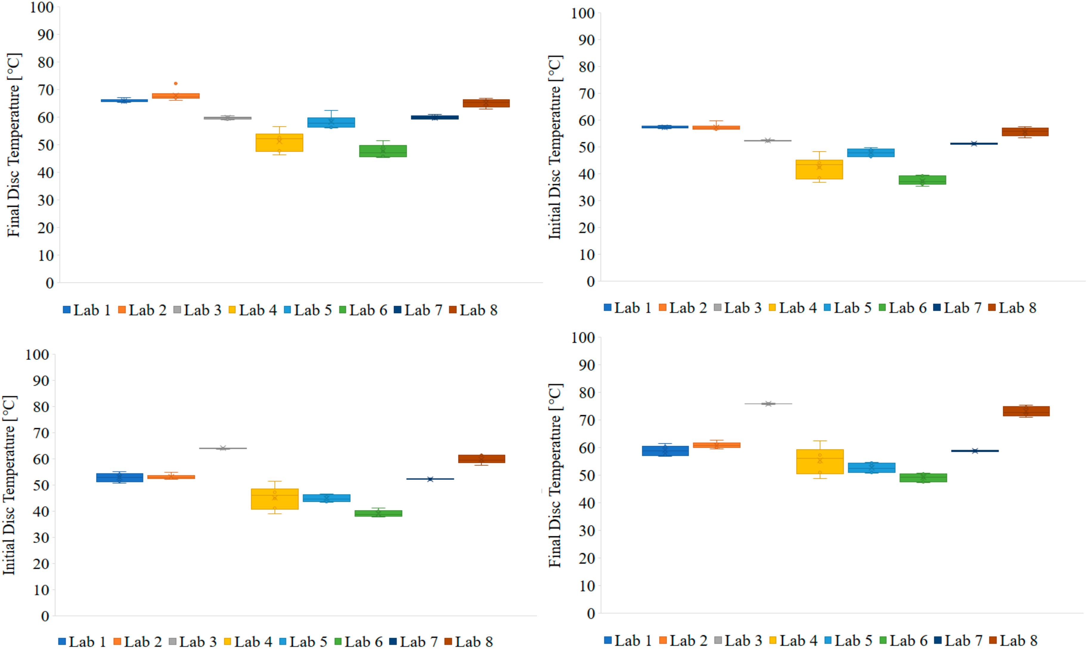
Table 5 provides the summary standard deviations for main measurands as a per cent of the average as calculated based on the application of robust methods. These include metrics for standard deviations for repeatability s r j * , sample effect s H j * , lab effect s L j * , and reproducibility s R j * . The statistics indicate values for all levels combined (303 brake events), for the 50th and the 95th percentiles, and each trip. The values in Table 5 indicate the per cent of the general average for all events, the 50th percentile, and the 95th percentile values. Moreover, the table provides the values as per cent of the general average for each trip. More details regarding the application of the equations, as well as examples with calculations, are provided in the PMP Brake Emissions Protocol—Part 1 [22].
Table 5 shows that the repeatability standard deviation s r j * is less than 1% of the mean values for braking speed and deceleration, as well as for the maximum brake temperature (regardless of the measurement method) and the cooling air temperature. In general, it seems that the repeatability within the labs for most parameters is within reasonable ranges both for the whole cycle, as well as for individual trips. Regarding the variation between samples as expressed by s H j * , it follows the trends described for the repeatability standard deviation. Table 5 shows that only the maximum temperature measured with TCRub exhibited relatively high variation (between 15% and 25% of the mean value) between labs, while all other parameters showed no significant difference between T1 and T2 (below 0.5% of the mean value for control parameters: Braking speed, braking deceleration, and braking torque). When studying the standard deviation for the between laboratory effect s L j * it seems that most parameters come with relatively high values. More specifically, deceleration and maximum brake temperature standard deviations are frequently higher than 15%. In contrast, the standard deviation of cooling air parameters depends on whether the examination includes all labs or only the ones with conditioned air for temperature and humidity. Finally, the standard deviation for reproducibility seems to be at an acceptable level. It is again the maximum temperature that comes with relatively high values, regardless of the measurement method, while deceleration seems to be less reproducible compared to the rest of the examined parameters.

3.2. Brake Temperature Study

3.2.1. Influence of Driving Conditions on Brake Temperature

One topic for investigation is the behaviour of the brake system under different driving conditions. Most braking events during the WLTP–Brake cycle—but also in real life—occur under urban conditions. Therefore, it is essential to understand how the brake system behaves in terms of its temperature under such conditions. Figure 5 illustrates the average, initial, final, and maximum disc temperature recorded for all labs at urban, rural, and motorway conditions over the R1 of T1. Temperatures were measured by utilising TCEmb. The remaining five repetitions (R2 to R6) of the cycle during T1 were comparable to R1; therefore, conclusions drawn from Figure 5 can be generalised.
Figure 5 shows that labs exhibited a relatively uniform behaviour in terms of disc temperature despite the differences in the execution of the WLTP–Brake cycle described in the previous paragraphs. Lab 6 exhibited an overall slightly lower average and initial brake temperatures compared to the other labs. On the other hand, Labs 2 and 5 seem to correlate with slightly higher final and peak temperatures; however, differences are within a few °C. Overall, rural driving correlates with a higher average, initial, and final disc temperature. Urban driving comes with relatively low final braking average temperature (~50–70 °C), and most importantly, with low maximum disc temperature (~150 °C). This lower temperature can indicate reduced Particle Number (PN) emissions in urban environments [32].
On the contrary, motorway driving correlates with low initial but with higher final and maximum braking temperatures. This higher temperature behaviour derives from the high-energy braking events taking place over motorway driving. This kind of event results in a higher increase of the brake temperature during the braking procedure than lower energy events observed over Urban and rural driving. Average (EED data at 1 Hz) and initial braking temperatures (EEC data at braking speed) exhibit small differences from each other and follow the same ranking in descending order: rural, urban, and motorway.

3.2.2. Influence of Cooling Air Parameters on Brake Temperature

One parameter with a significant influence on the brake temperature profile is the incoming cooling air. The proper control of the cooling air temperature and RH allows the lab to minimise uncertainty during testing. TF1 has agreed on applying an incoming cooling air temperature of (20 ± 2) °C and RH of (50 ± 5) % RH on average for the entire test. Table 6 presents the average incoming cooling air temperature and RH (and the 95% limits over the repetition) for all labs in T1 (per EED files). All values in red indicate non-compliance with the requested value for the incoming cooling air temperature.
Table 6 shows that five labs managed to stay within the specification of (20 ± 2) °C for the incoming cooling air’s mean temperature. On the other hand, Labs 4 and 6 ran T1 with a mean cooling air temperature approximately 10 °C lower than the target value, while Lab 8 was approximately 10 °C higher than the target value. However, to verify whether the labs really managed to comply with the cooling air temperature specification one needs to look to the individual repetitions rather than the mean values. From this assessment, it seems that only Labs 1, 2, and 3 managed to comply with the specification during all six repetitions. On the other hand, Labs 5 and 7 seem to comply when considering the average values (19.2 °C and 19.7 °C, respectively); however, fail to maintain the temperature regime within the defined threshold for one or more individual repetitions. For instance, Lab 5 managed to keep the average temperature of the incoming cooling air during R1 to 19.6 °C; however, instantaneous values deviated between 8.4 °C and 26.3 °C. This information can only be retrieved from the detailed report and not the averaged values depicted in Table 6. Similarly, R1 and R5 of Lab 7 did not follow the temperature specification with the deviations ranging between 9.2 °C and 30.2 °C, and this is reflected in the high 95 percentile of the average values. Such high temperature fluctuations may influence the brake temperature profile and result in a defective test for brake emissions. Labs 4, 6, and 8 were 10 °C below or above the target temperature both in terms of average value and within the individual runs.
Table 6 shows that only five labs managed to stay within the specification of (50 ± 5) % for the mean RH of the incoming cooling air. However, like with the cooling air temperature, there is a need to assess the behaviour within each individual repetition to understand whether RH control was successful. A very good example of the need for such an assessment is Lab 7. Despite meeting the target RH in terms of the mean averaged value (49.4%), it failed to comply during all individual repetitions. This behaviour was due to the RH’s very high fluctuation during the tests and highlighted the necessity of examining repetitions separately and not only as a whole. For some friction couples, such deviations may influence the coefficient of friction and the properties of the air transporting the aerosol (brake debris) to the instrument cluster.
After examining all individual repetitions, only Labs 1 and 2 managed to stay within the specification for the whole T1. Lab 4 failed to maintain the average RH within the defined limits over R4, R5, and R6. A good example is R4 which was within the predefined limits only for 13% of the time. In this case, RH was substantially higher than the requested 50% and reached values up to 70%. Labs 7 and 8 failed to comply with the average RH specification for all repetitions. On the other hand, Lab 3 seems to control the RH properly; however, not within the 5% threshold. The average value remains almost constant and very close to the target 50%, while the tests’ deviations are marginally higher than 5%. This deviation indicates a possible need to relax the ±5% threshold or introduce a predefined period allowing deviations from this value.
The following analysis uses data from Lab 4 to study the influence of the incoming cooling air temperature on the brake temperature profile. Another advantage of using data from only one lab is to keep the rest of the testing parameters constant during all repeats. This approach allows the assignment of observed differences in the brake temperature primarily to the conditions for the incoming cooling air temperature. Figure 6 depicts the average disc temperature recorded in each one of the six repetitions of T1. The results include both TCEmb (blue marks) and TCRub (red marks), while polynomial fits are indicative and do not correspond to any model for convective heat transfer.
Despite the temperature difference in the readings of the two TCs, there seems to be a similar trend for both variants. Figure 6 shows that reducing cooling air temperature results in a reduction of average disc temperature. It seems that the reduction of the average disc temperature is not directly proportional to the reduction of cooling air temperature. More specifically, cooling the incoming air by approximately 8.5 °C induces a reduction of the disc temperature between 10 °C and 15 °C. This is expected as convective heat transfer is non-linear. Overall, it is evident that the laboratory needs to strictly control the temperature of the incoming cooling air to be able to follow the target temperature profile.
The difference is also apparent when examining the 1 Hz data for the disc temperature. Table 6 shows that R2 and R3 of Lab 4 exhibited a performance comparable for cooling air temperature and RH, resulting in identical average disc temperatures. Figure 7 (left-hand side) depicts this well, illustrating the disc temperature profile of the two repetitions throughout the entire cycle. The two repetitions resulted in identical disc temperature profiles over the whole duration of the cycle. On the other hand, Figure 7 (right-hand side) illustrates the differences between R2 (red line) and R5 (purple line), especially for temperatures below 60 °C. In this case, R2 was conducted with an average cooling air temperature of 13.4 °C, resulting in generally higher disc temperatures. In comparison, R5 was performed with an average cooling air temperature of 8.4 °C and resulted in significantly lower disc temperatures. Moreover, it is imperative to take into account the fact that R5 ran with 20% higher RH than R2.

3.2.3. Influence of the Temperature Measurement Method on Brake Temperature

Brake disc temperature was measured using TCEmb and TCRub. The two methods provide neither the same readings nor the same level of accuracy in the measurement of disc temperature. Figure 8 illustrates the mean of the average values (middle line of the box) for each one of the six repetitions of T1 for initial, final and maximum disc temperature. The median divides the box into a bottom half and a top half. The bottom line of the box represents the first quartile. The top line of the box represents the third quartile. The whiskers (vertical lines ending with a dash) extend from each end of the box to the minimum value and the maximum value. Statistics for all labs came from the corresponding EEC files. The boxplot graphs show both TCEmb (left-hand side panels) and TCRub (right-hand side panels) measurement values for comparison purposes.
Figure 8 shows that the mean of the average initial brake temperature for each of the six repetitions measured with the TCEmb fall within a 20 °C difference (~40–60 °C). For measurements using TCRub the mean temperature values lie within a slightly broader range of 25 °C (~40–65 °C). When the labs that managed to regulate the incoming cooling air at (20 ± 1) °C and (50 ± 5) % RH are considered (Labs 1, 2, 3, 5 and 7), then mean TCEmb values fall within a narrow range of less than 10 °C (~50–60 °C). On the other hand, the range of mean temperature values measured utilising TCRub does not improve significantly and lies within 20 °C (~45–65 °C). Similar to the initial temperatures, the mean brake temperature values measured with the TCEmb fall again within a 20 °C difference (~50–70 °C). For the TCRub, the mean final temperature values lie within a broader range of approximately 30 °C (~50–80 °C). Again, considering only the labs that regulated the incoming cooling air, TCEmb mean values fall within a relatively narrow range of 10 °C (~60–70 °C). On the other hand, the means values for TCRub for final temperature do not exhibit a significant improvement, falling within a 25 °C range (~50–75 °C). These findings provide the first indication that TCEmb gives more precise temperature measurements compared to TCRub.
Examination of mean values of the averaged maximum disc temperature confirms the previous statement; temperature measurements employing TCEmb are more robust and repeatable compared to TCRub. The bottom panels in Figure 8 clearly illustrate that the mean maximum temperature values measured with the TCEmb are very close to each other for most of the labs and lie within a 30 °C range. On the other hand, the average values for the maximum temperature values measured with the TCRub deviate significantly among the labs and lie between 55 °C and 60 °C (i.e., Maximum Temperature between Lab 3 and Lab 4). The assessment above concludes that temperature measurement and subsequent analysis shall use only TCEmb. The same tests with TCRub can result in twice as high deviations.
Figure 9 depicts the disc final temperature profile for all 303 brake events of the R1–T1 using TCEmb (left-hand side) and TCRub (right-hand side), respectively. Both figures include only the labs that were able to control the temperature and humidity of the incoming cooling air as requested. Temperature measurement with TCEmb is more robust and exhibits a lower deviation among the labs, remaining mostly below 20 °C for all braking events. In comparison, TCRub provides readings with deviations between labs of up to 50 °C, especially for high energy braking events close to the end of the WLTP–Brake cycle.

3.2.4. Influence of the Initial Cycle Temperature on the Brake Temperature Profile

Labs were requested to start each one of the 10 trips within the WLTP–brake cycle from the initial brake temperature of 25 °C. After each trip, the cycle includes a soak time to cool down and reach the target temperature, which shall represent the ambient temperature during the vehicle test. The soak time varied significantly between the trips of the cycle depending on the level of temperature reached over the previous trip. Moreover, soak time varied significantly also among the labs, due to the difference among the setups and the application of different cooling air flowrates. Table 7 gives an overview of the soak times applied by different labs in all repetitions of T1. For Lab 3, it was not possible to calculate the exact soak times, due to some issues with the EED files. Soak times are provided in [h], while values in parenthesis represent the percentage (%) of total soak time over the whole duration of the test.
The application of different initial disc temperature at the beginning of each repetition influences the average disc temperature over the cycle. Figure 10 illustrates the average (left) and maximum (right) disc temperature over the cycle measured by TCEmb plotted against the disc temperature at the beginning of the cycle. From the evidence presented, it seems that increasing the disc temperature at the beginning of the cycle increases the average brake temperature over the cycle. Lab 6 seems to behave differently in terms of temperature regimes (generally lower average temperatures) compared to the other labs, due to the different cooling strategy (application of constant airspeed of 45 km/h). However, Lab 6 seems to follow the same direction regarding the influence of temperature at the beginning of the cycle to the average brake temperature.
A remarkable find is that the application of different initial disc temperature at the beginning of the cycle does not seem to influence the maximum disc temperature over the cycle. Figure 10 shows that most of the tests were performed with an initial disc temperature of approximately 20–25 °C and resulted in maximum disc temperature in a wide range of 150–190 °C. Moreover, Lab 4 that performed tests with entirely different initial disc temperature resulted in maximum disc temperature of approximately 160 °C, regardless of the initial cycle temperature. It seems that other parameters are affecting maximum temperature rather than the temperature at the beginning of the cycle, and thus, the correct application of soak times.
Moving forward, all labs need to follow a strict soaking protocol to avoid differences in the temperature regime and conduct repeatable and reproducible tests. The proper soak applies even if maximum temperature—and thus, PN emissions—does not seem to be affected by the correct application of soaking.

4. Conclusions

The increasing relevance of brake particle emissions to overall ambient PM concentrations renders the development of a standardised method for measuring brake particle emissions of utmost importance. The execution of interlaboratory (Round-Robin) studies is a regular practice when setting-up a standardised method. This kind of studies allows for useful conclusions to be drawn and helps bring forward suggestions for improvement of the suggested methodologies. The main achievement of the current exercise was the elaboration and submission of several proposals related to the development of the PMP Brake Protocol for measuring brake particle emissions [22]. Several parameters have been found to influence the correct application and execution of the WLTP–brake cycle. The most important are summarised below:
  • Dyno control strategy—it is important to properly control the speed traces during the application of the WLTP–brake Cycle. Brake speed and deceleration are heavily influenced by the dyno control strategy and incorrect control might lead to false execution of brake events. This phenomenon is more pronounced in urban braking events.
  • Parasitic losses—it is important for the labs to apply proper corrections to reduce the total torque demand from the foundation brake to reflect the vehicle’s resistive forces. No standard method for correcting for the parasitic losses exists. For that reason, a detailed proposal has been submitted to the GRPE Informal Working Document 81-12 [22].
  • Incoming cooling air temperature—it heavily affects the brake temperature profile. Thus, it is necessary to strictly control this parameter during the execution of the WLTP–brake cycle. It is proposed to set cooling air temperature during the test within (20 ± 2) °C. Furthermore, it is proposed to allow for a more relaxed limit of (20 ± 5) °C for up to 5% of the duration of the WLTP–Brake cycle.
  • Incoming cooling air relative humidity—it seems to affect brake temperature profile; however, it was not possible to quantify its effect within the current exercise. It is proposed to set cooling air RH during the test within (50 ± 5) °C. Additionally, it is proposed to allow for a more relaxed limit of (50 ± 10) °C for up to 5% of the duration of the WLTP–Brake cycle.
  • Incoming cooling airspeed—different test setups feature entirely different geometries leading to incomparable cooling conditions for the brake system. This heavily affects the brake temperature profile. There is a need to establish a commonly accepted methodology to adjust the airstream speed to provide comparable thermal regimes across facilities. A detailed proposal has been submitted to the GRPE Informal Working Document 81-12 [22].
  • Soaking protocol—brake temperature at the beginning of each trip influences the temperature profile during the trip. Labs need to follow a strict soaking protocol to avoid differences in the temperature regime and conduct repeatable and reproducible tests. The proper soak applies even if maximum temperature—and thus, PN emissions—does not seem to be affected by the correct application of soaking.
  • Temperature measurement method—the selection of the proper instrumentation has a significant impact on the temperature regimes. TCEmb provides more accurate measurements compared to TCRub. Thus, TCEmb is the preferable option for temperature measurements during emission tests.
Apart from parameters affecting the correct execution of the WLTP–brake cycle it was possible to extract useful conclusions related to the brake temperature, which is recognised as one of the most critical parameters influencing particle emissions.
  • Urban driving correlates with relatively low final and maximum braking temperature. This trend possibly points to generally lower Particle Number (PN) emissions in urban environments. This assumption shall be further analysed and confirmed through actual emissions testing.
  • Rural driving is linked to high average, initial and final disc temperatures. This possibly indicates relatively high brake emissions in rural environments; however, other parameters like the braking frequency shall be taken into account.
  • Motorway driving correlates with high final and maximum braking temperatures. This higher temperature behaviour occurs during the high-energy braking events taking place over motorway driving.
  • A remarkable find is that the application of different initial disc temperature at the beginning of the cycle does not seem to influence the maximum disc temperature over the cycle. This allows for a relaxation of the set temperature value for the beginning of the test from 25 °C to 35 °C.

Author Contributions

Conceptualization, T.G. and J.G.; data curation, T.G., C.A., A.H. and R.V.; formal analysis, C.A. and A.H.; investigation, T.G., S.G., M.R., G.P., A.S., A.G., A.P., M.Z., S.A. and M.M.; methodology, T.G., C.A., J.G., S.G., M.R., G.P., A.S., A.G., A.P., S.A. and R.V.; supervision, J.G.; validation, C.A., S.G., M.R., G.P., A.S., A.G. and M.M.; visualization, M.R., A.G. and A.S.; writing—original draft, T.G.; writing—review and editing, T.G., C.A., J.G., G.P. and M.M. All authors have read and agreed to the published version of the manuscript.

Funding

This research received no external funding.

Conflicts of Interest

The authors declare no conflict of interest.

References

  1. Environment Directorate—Environment Policy Committee. Non-exhaust Emissions from Road Transport. Causes, Consequences and Policy Responses; OECD—Organization for Economic Co-Operation and Development: Paris, France, 2020. [Google Scholar]
  2. UK Air Quality Expert Group; Department for Environment, Food and Rural Affairs—Scottish Government—Welsh Government—Department of the Environment in Northern Ireland. Non-exhaust Emissions from Road Traffic; PB14581 (2019). Available online: https://uk-air.defra.gov.uk/library/reports.php?report_id=992 (accessed on 1 December 2020).
  3. Grigoratos, T.; Martini, G. JRC Scientific and Policy Reports. Non-Exhaust Traffic Related Emissions. Brake and Tyre Wear PM; Publications Office of the European Union: Luxembourg, 2014. [Google Scholar] [CrossRef]
  4. Gerlofs-Nijland, M.; Bokkers, B.; Sasche, H.; Reijnders, J.; Gustafsson, M.; Boere, A.; Fokkens, P.; Leseman, D.; Augsburg, K.; Cassee, F. Inhalation toxicity profiles of particulate matter: A comparison between brake wear with other sources of emission. Inhal. Toxic. 2019, 31, 89–98. [Google Scholar] [CrossRef]
  5. Volta, A.; Sforzini, S.; Camurati, C.; Teoldi, F.; Maiorana, S.; Croce, A.; Benfenati, E.; Perricone, G.; Lodi, M.; Viarengo, A. Ecotoxicological effects of atmospheric particulate produced by braking systems on aquatic and edafic organisms. Environ. Int. 2020, 137, 105564. [Google Scholar] [CrossRef]
  6. Grigoratos, T.; Martini, G. Brake wear particle emissions: A review. Environ. Sci. Pollut. Res. 2015, 22, 2491–2504. [Google Scholar] [CrossRef] [PubMed] [Green Version]
  7. Wahlström, J.; Lyu, Y.; Matějka, V.; Söderberg, A. A pin-on-disc tribometer study of disc brake contact pairs with respect to wear and airborne particle emissions. Wear 2017, 384–385, 124–130. [Google Scholar] [CrossRef]
  8. Alemani, M.; Nosko, O.; Metinoz, I.; Olofsson, U. A study on emission of airborne wear particles from car brake friction pairs. SAE Int. J. Mater. Manuf. 2015, 9, 147–157. [Google Scholar] [CrossRef]
  9. Hagino, H.; Oyama, M.; Sasaki, S. Laboratory testing of airborne brake wear particle emissions using a dynamometer system under urban city driving cycles. Atmospheric Environ. 2016, 131, 269–278. [Google Scholar] [CrossRef] [Green Version]
  10. Agudelo, C.; Deacon, P.; Marschall, M.; Markiewicz, R.; Hortet, A.; Tiwari, A.; Anderson, R. Systematic assessment of brake emissions during dynamometer tests. In Proceedings of the EuroBrake2017 Conference, Dresden, Germany, 2–4 May 2017. [Google Scholar]
  11. Gramstat, S.; Cserhati, A.; Lugovyy, D.; Schroder, M. Investigations of brake particle emissions—Testing method, vehicle peculiarities and friction material influence. In Proceedings of the EuroBrake2017 Conference, Dresden, Germany, 2–4 May 2017. [Google Scholar]
  12. Mamakos, A.; Arndt, M.; Hesse, D.; Augsburg, K. Physical characterization of brake-wear particles in a PM10 dilution tunnel. Atmosphere 2019, 10, 639. [Google Scholar] [CrossRef] [Green Version]
  13. Mathissen, M.; Grochowicz, J.; Schmidt, C.; Vogt, R.; zum Hagen, F.H.; Grabiec, T.; Steven, H.; Grigoratos, T. A novel real-world braking cycle for studying brake wear particle emissions. Wear 2018, 414–415, 219–226. [Google Scholar] [CrossRef]
  14. Perricone, G.; Matějka, V.; Alemani, M.; Valota, G.; Bonfanti, A.; Ciotti, A.; Olofsson, U.; Söderberg, A.; Wahlström, J.; Nosko, O.; et al. A concept for reducing PM10 emissions for car brakes by 50%. Wear 2018, 396–397, 135–145. [Google Scholar] [CrossRef]
  15. Perricone, G.; Matĕjka, V.; Alemani, M.; Wahlström, J.; Olofsson, U. A test stand study on the volatile emissions of a passenger car brake assembly. Atmosphere 2019, 10, 263. [Google Scholar] [CrossRef] [Green Version]
  16. Chasapidis, L.; Grigoratos, T.; Zygogianni, A.; Tsakis, A.; Konstandopoulos, A. Study of brake wear particle emissions of a minivan on a chassis dynamometer. Emiss. Control. Sci. Technol. 2018, 4, 271–278. [Google Scholar] [CrossRef] [Green Version]
  17. Mathissen, M.; Grigoratos, T.; Lahde, T.; Vogt, R. Brake wear particle emissions of a passenger car measured on a chassis dynamometer. Atmosphere 2019, 10, 556. [Google Scholar] [CrossRef] [Green Version]
  18. Mathissen, M.; Scheer, V.; Vogt, R.; Benter, T. Investigation on the potential generation of ultrafine particles from the tire-road interface. Atmos. Environ. 2011, 45, 6172–6179. [Google Scholar] [CrossRef]
  19. Kwak, J.H.; Kim, H.; Lee, J.; Lee, S. Characterization of non-exhaust coarse and fine particles from on-road driving and laboratory measurements. Sci. Total. Environ. 2013, 458–460, 273–282. [Google Scholar] [CrossRef]
  20. Zum Hagen, F.H.F.; Mathissen, M.; Grabiec, T.; Hennicke, T.; Rettig, M.; Grochowicz, J.; Vogt, R.; Benter, T. Study of brake wear particle emissions: Impact of braking and cruising conditions. Environ. Sci. Technol. 2019, 53, 5143–5150. [Google Scholar] [CrossRef]
  21. Hesse, D.; Augsburg, K.; Kuhn, U.; Leicht, R. Influence of regenerative braking on the emission behavior of friction brakes. In Proceedings of the 48th PMP Meeting, Joint Research Centre, Ispra, Italy, 7–8 November 2018; Available online: https://wiki.unece.org/display/trans/PMP+48th+session (accessed on 1 December 2020).
  22. UNECE (2020)—Informal Document GRPE-81-12 (2020). (PMP) Brake Emissions Protocol—Part 1. Available online: https://www.unece.org/trans/main/wp29/wp29wgs/wp29grpe/grpeinf81.html (accessed on 1 December 2020).
  23. EKB—European Brake Noise Experts Group. VDA—EKB 3008 Data Exchange Format. Version in April 2013. Available online: https://www.vda.de/en/services/Publications.html (accessed on 1 December 2020).
  24. Valverde Morales, V.; Bonnel, P. On-Road Testing with Portable Emissions Measurement Systems (PEMS)—Guidance Note for Light-Duty Vehicles; Publications Office of the European Union: Luxembourg, 2018; ISBN 978-92-79-77345-7. [Google Scholar] [CrossRef]
  25. Agudelo, C.; Vedula, P.; Bautell, J.; Stanard, A.; DeFreis, T. Thermal and braking regimes during proving ground measurements using the wltp-brake cycle for brake emissions measurements. In Proceedings of the EuroBrake2019 Conference, Dresden, Germany, 21–24 May 2019. [Google Scholar]
  26. Cantrell, C.A. Technical note: Review of methods for linear least-squares fitting of data and application to atmospheric chemistry problems. Atmospheric Chem. Phys. Discuss. 2008, 8, 5477–5487. [Google Scholar] [CrossRef] [Green Version]
  27. UNECE Amendment 5 to UN GTR. No.15—Amendment 5 to UN Global Technical Regulations Concerning the Worldwide Harmonized Light Vehicles Test Procedure (WLTP). 2019. Available online: https://www.unece.org/trans/main/wp29/wp29wgs/wp29gen/wp29glob_registry.html (accessed on 1 December 2020).
  28. SAE. Drive Quality Evaluation for Chassis Dynamometer Testing; SAE International: Warrendale, PA, USA, 2014. [Google Scholar]
  29. ISO. Accuracy (Trueness and Precision) of Measurement Methods and Results—Part 1: General Principles and Definitions; International Organization for Standardization (ISO): London, UK, 1994. [Google Scholar]
  30. ISO. Accuracy (Trueness and Precision) of Measurement Methods and Results—Part 5: Alternative Methods for the Determination of the Precision of a Standard Measurement Method; ISO 5725-5:1998; International Organization for Standardization (ISO): London, UK, 1998. [Google Scholar]
  31. ISO. Accuracy (Trueness and Precision) of Measurement Methods and Results—Part 2: Basic Method for the Determination of Repeatability and Reproducibility of a Standard Measurement Method; ISO 5725-2:2019; International Organization for Standardization (ISO): London, UK, 1998. [Google Scholar]
  32. Alemani, M.; Wahlström, J.; Olofsson, U. On the influence of car brake system parameters on particulate matter emissions. Wear 2018, 396–397, 67–74. [Google Scholar] [CrossRef]
Figure 1. Schematic hierarchy of Labs (Lab 1–Lab 8), Tests (T1 and T2), Repeats (R1–R6) and Trips (Trip #1–Trip #10).
Atmosphere 11 01309 g001
Figure 2. Plots for deceleration versus speed bias (left-hand side) and scatter (right-hand side) for all labs compared to the WLTP–brake cycle.
Atmosphere 11 01309 g002
Figure 3. Histograms for all decelerations during T1‒R1 for Lab 1 and Lab 3 and the nominal WLTP–brake cycle—the continuous lines represent the lognormal distribution for each dataset.
Atmosphere 11 01309 g003
Figure 4. Deceleration by event for each lab (T1-R1), the vehicle, and the overall average. The solid grey line identifies the ideal regression line (vehicle). The dataset with a regression line yavg = 1.0786x + 0.0413 indicates the general average excluding Lab 6.
Atmosphere 11 01309 g004
Figure 5. Average, initial, final, and maximum disc temperature for all labs at urban, rural, and motorway conditions over the R1 of T1—data includes time-resolved temperature extracted at 1 Hz from the EED files for the entire WLTP Brake cycle.
Atmosphere 11 01309 g005
Figure 6. Average brake temperature from EED file at 1 Hz as a function of incoming air temperature—the trendlines represent polynomial models for both variants.
Atmosphere 11 01309 g006
Figure 7. Disc temperature profile measured by TCEmb for Lab 4 during T1. Left-hand side depicts R2 (red line) vs R3 (purple line). Right-hand side depicts R2 (red line) vs R5 (purple line).
Atmosphere 11 01309 g007
Figure 8. Boxplots for the average disc temperatures—the plots illustrate values for initial (upper panels), final (middle panels), and maximum (bottom panels) temperatures.
Atmosphere 11 01309 g008aAtmosphere 11 01309 g008b
Figure 9. Final disc temperature profile measured by TCEmb (left-hand side) and TCRub (right-hand side) for R1 during T1.
Atmosphere 11 01309 g009
Figure 10. Average (left-hand side) and maximum (right-hand side) disc temperature over the WLTP–brake cycle plotted against the disc temperature at the beginning of the cycle.
Atmosphere 11 01309 g010
Table 1. Summary of the applied hardware and testing conditions—green cells indicate the lab followed the recommended method. Orange cells indicate the lab used an acceptable or equivalent method. Red cells point to significant deviations. Cells with (*) indicate tests not completed.
Item or ConditionLab 1Lab 2Lab 3Lab 4Lab 5Lab 6Lab 7Lab 8
T1T2T1T2T1T2T1T2T1T2T1T2T1T2T1T2
Dynamometer [1 = Performance, 2 = NVH, 3 = Emissions]1121111111221*3 #*
Climate Control [1 = Temp. and RH, 2 = Temp. only, 3 = Fresh]1111113111221*3*
Control programme [1 = Ford, 2 = Link US, 3 = Lab specific]2212332211332*3*
Cooling air adjustment [1 = 2 curves, 2 = Trip #10, 3 = Other]2211111211332*1*
Test plan [1 = 2 successful tests, 2 = 1 successful test]1111111111112*2*
Pads [1= RR batch–New, 2 = RR batch—used, 3 = Dummies]1212121212121*3*
Disc [1= RR batch–New, 2 = RR batch—used, 3 = Dummies]1212121212121*3*
Disc temperature method [1 = TCRub, 2 = TCEmb, 3 = Both]3333333333333*3*
Temperature control for soak application [1 = TCRub, 2 = TCEmb]1111111111112*1*
# Single-ended performance dynamometer adapted for emission measurements.
Table 2. Average and 95th percentile limits for braking speed and deceleration—data split into Total, Urban, Rural, and Motorway events.
LabBraking Speed [km/h]Total Deceleration [m/s2]
AllUrbanRuralMotorwayAllUrbanRuralMotorway
WLTP41.133.873.1102.60.970.931.171.25
Lab 141.8 ± 0.136.5 ± 0.163.0 ± 0.184.3 ± 0.11.31 ± 0.011.26 ± 0.021.47 ± 0.011.70 ± 0.01
Lab 241.4 ± 0.236.8 ± 0.261.3 ± 0.273.0 ± 0.20.89 ± 0.080.84 ± 0.101.13 ± 0.001.14 ± 0.00
Lab 341.4 ± 0.333.8 ± 0.372.2 ± 0.2102.1 ± 0.20.98 ± 0.030.94 ± 0.031.18 ± 0.021.26 ± 0.02
Lab 441.4 ± 0.133.8 ± 0.172.1 ± 0.1102.0 ± 0.11.22 ± 0.001.18 ± 0.001.45 ± 0.001.49 ± 0.01
Lab 541.3 ± 0.335.2 ± 0.367.6 ± 0.382.2 ± 0.30.89 ± 0.080.84 ± 0.091.17 ± 0.001.17 ± 0.00
Lab 637.1 ± 0.329.5 ± 0.367.6 ± 0.397.4 ± 0.30.88 ± 0.030.83 ± 0.031.07 ± 0.021.13 ± 0.02
Lab 741.5 ± 0.133.9 ± 0.172.1 ± 0.2102.0 ± 0.20.84 ± 0.010.80 ± 0.010.98 ± 0.011.02 ± 0.01
Lab 841.4 ± 0.133.7 ± 0.172.1 ± 0.0102.0 ± 0.10.98 ± 0.010.94 ± 0.011.18 ± 0.011.25 ± 0.01
Table 3. Summary of speed violations for all six repetitions during T1 for all labs—the % values indicate the amount of time during the entire cycle that the dynamometer speed was outside the ±2 km/h threshold. (*) denotes missing data.
LabSpeed Violations Per Repeat [%]Mean [%]
R1R2R3R4R5R6
L120.17.67.87.76.67.99.6
L211.22.12.22.32.53.03.9
L340.644.042.443.139.843.442.2
L41.00.20.10.00.90.40.4
L51.72.23.02.2**1.5
L60.00.00.00.00.00.00.0
L710.110.210.810.810.29.410.3
L838.938.437.537.737.60.531.8
Mean15.413.113.013.012.28.112.6
Table 4. Summary of RMSSE and % RMSSE values for T1 for all labs—mean values include only the actual lab results. (*) denotes missing data.
LabRMSSE [km/h]Mean [km/h]
R1R2R3R4R5 R6
WLTP3.23.23.23.23.23.23.2
L15.4 (170%)2.8 (87%)2.8 (87%)2.8 (87%)2.7 (86%)2.8 (89%)3.2 (100%)
L216.8 (526%)2.8 (87%)2.8 (88%)2.8 (89%)2.8 (89%)3.0 (93%)5.2 (162%)
L313.7 (428%)14.8 (464%)13.9 (435%)14.4 (451%)13.0 (407%)13.6 (428%)13.9 (435%)
L41.5 (47%)1.2 (38%)1.1 (34%)1.2 (36%)1.5 (46%)1.4 (43%)1.3 (41%)
L52.6 (82%)2.8 (88%)3.0 (94%)2.9 (90%)**2.8 (89%)
L60.5 (15%)0.3 (11%)0.7 (21%)0.6 (18%)0.6 (19%)0.4 (14%)0.5 (16%)
L73.2 (100%)3.4 (108%)3.5 (110%)3.6 (113%)3.2 (101%)3.0 (93%)3.3 (104%)
L816.3 (511%)15.8 (495%)15.7 (491%)15.7 (491%)15.9 (500%)1.2 (37%)13.4 (421%)
Mean7.5 (235%)5.5 (172%)5.4 (170%)5.5 (172%)5.7 (178%)3.6 (114%)5.5 (174%)
Table 5. Summary standard deviations for main measurands as a per cent of the average.
MeasurandMetricMeanPercentilesTrip
12345678910
Number of Levels (Brake Events)
30350th95th29422818492687114
Standard Deviation [% of the Mean for the Applicable Range of Data]
Braking speed [km/h] s r j * 0.10.10.10.20.10.10.10.10.30.10.10.20.1
s H j * 0.00.10.10.10.00.0-0.0-0.00.00.10.0
s L j * 4.24.42.35.44.23.83.13.611.03.33.27.84.6
s R j * 0.40.40.30.50.40.30.30.31.70.30.30.90.5
Average-by-distance deceleration [m/s2] s r j * 0.30.30.30.40.30.30.20.30.40.20.30.30.2
s H j * 0.20.20.30.10.10.20.10.11.60.10.10.30.2
s L j * 17.616.116.919.418.117.416.817.014.918.016.717.717.1
s R j * 8.48.17.78.08.69.66.98.28.111.66.49.08.3
Average-by-distance torque [N·m] s r j * 0.30.20.30.40.30.20.20.20.30.10.20.20.2
s H j * 0.10.10.20.10.00.10.00.10.30.00.10.20.1
s L j * 6.75.77.16.66.57.56.27.010.45.66.15.96.7
s R j * 3.83.44.23.03.34.04.53.77.94.94.43.53.9
Average-by-distance pressure [kPa] s r j * 5.92.58.215.65.74.02.62.42.82.22.52.51.9
s H j * 1.92.32.1-1.12.31.72.41.81.71.70.92.2
s L j * 9.28.48.79.810.19.59.29.411.08.79.17.78.4
s R j * 10.99.610.918.610.810.310.09.311.59.89.58.68.9
Average-by-distance COF [µ] s r j * 5.12.610.312.86.34.32.63.03.12.32.62.42.2
s H j * 2.52.24.50.82.22.83.03.01.91.62.11.62.5
s L j * 8.27.010.710.18.98.27.16.89.05.96.87.68.2
s R j * 9.88.313.817.011.19.77.07.410.86.66.48.88.5
Maximum temperature with TCEmb [°C] s r j * 1.81.61.72.72.21.91.71.62.11.31.61.51.4
s H j * 2.92.82.73.52.53.72.73.24.03.43.24.12.4
s L j * 15.816.211.914.415.716.513.215.929.313.613.825.016.1
s R j * 16.517.212.615.016.216.814.117.222.213.115.022.116.8
Maximum temperature with TCRub [°C] s r j * 2.22.02.23.42.42.22.12.02.11.81.61.61.9
s H j * 5.75.84.96.45.46.15.25.510.03.95.47.65.8
s L j * 18.619.015.624.617.819.114.717.925.818.116.325.418.4
s R j * 17.918.015.623.917.115.414.417.021.818.115.927.918.0
Cooling air temperature (controlled) [°C] s r j * 1.11.01.41.51.20.90.91.01.01.01.11.10.9
s H j * 0.60.71.1-0.40.50.40.60.90.60.10.70.7
s L j * 1.51.22.63.21.01.01.21.2-1.51.51.11.2
s R j * 1.61.42.42.51.41.31.61.61.01.51.81.51.5
Cooling air temperature (all) [°C] s r j * 1.41.12.02.71.21.01.01.21.11.21.21.31.1
s H j * 1.21.32.00.41.11.10.91.21.91.40.51.41.4
s L j * 31.531.732.129.730.630.830.731.631.933.232.332.632.4
s R j * 4.23.18.79.22.82.73.33.31.34.13.93.53.4
Cooling air RH (controlled) [%RH] s r j * 3.52.96.67.13.52.42.23.12.83.32.63.32.9
s H j * 0.10.61.9------0.2--0.2
s L j * 1.11.02.82.51.20.70.60.81.80.50.60.70.9
s R j * 3.73.07.47.73.82.52.33.23.53.42.63.43.0
Cooling air RH (all) [%RH] s r j * 4.13.57.17.34.13.33.23.72.84.03.54.13.3
s H j * 0.20.92.1---------0.3
s L j * 8.78.89.97.07.47.68.19.29.410.09.710.09.3
s R j * 5.24.39.49.85.34.14.14.64.45.24.35.04.3
Table 6. Averaged temperature and RH of incoming air for T1—cells in red indicate non-compliant repeats and with an (*) data not available for that repeat.
Temperature [°C]
Lab 1Lab 2Lab 3Lab 4Lab 5Lab 6Lab 7Lab 8
R120.0 ± 1.420.0 ± 0.819.8 ± 0.515.0 ± 1.319.2 ± 2.511.2 ± 0.319.6 ± 3.430.9 ± 0.8
R220.0 ± 1.520.0 ± 1.419.8 ± 0.313.4 ± 0.619.2 ± 0.111.0 ± 0.119.7 ± 0.428.2 ± 2.1
R320.1 ± 0.820.0 ± 1.019.9 ± 0.313.4 ± 0.819.2 ± 0.110.8 ± 0.319.7 ± 0.926.8 ± 0.6
R420.0 ± 1.320.0 ± 1.019.8 ± 0.311.5 ± 5.119.2 ± 0.110.9 ± 0.419.7 ± 0.730.8 ± 3.0
R520.0 ± 1.420.0 ± 1.019.9 ± 0.58.4 ± 0.8*10.6 ± 0.219.6 ± 3.329.6 ± 2.1
R619.9 ± 1.520.0 ± 1.419.8 ± 0.46.5 ± 1.2*10.5 ± 0.119.7 ± 0.830.2 ± 2.2
Mean20.0 ± 0.120.0 ± 0.019.8 ± 0.011.4 ± 6.519.2 ± 0.010.2 ± 0.519.7 ± 0.129.4 ± 3.2
Relative Humidity [%RH]
Lab 1Lab 2Lab 3Lab 4Lab 5Lab 6Lab 7Lab 8
R150.0 ± 3.950.0 ± 3.349.5 ± 9.350.5 ± 2.949.6 ± 6.1*48.5 ± 15.138.0 ± 4.4
R250.0 ± 3.950.1 ± 3.850.0 ± 5.352.2 ± 1.450.1 ± 0.7*50.5 ± 10.940.9 ± 1.3
R350.0 ± 3.750.0 ± 2.949.7 ± 5.951.2 ± 3.150.0 ± 0.5*48.3 ± 16.343.8 ± 1.8
R450.0 ± 4.050.1 ± 3.150.2 ± 5.059.7 ± 23.550.1 ± 0.7*51.2 ± 14.836.7 ± 8.7
R550.0 ± 4.050.0 ± 3.050.1 ± 5.670.7 ± 2.8**49.3 ± 17.041.8 ± 6.9
R650.0 ± 3.950.2 ± 4.749.7 ± 5.464.1 ± 4.4**48.7 ± 18.342.2 ± 4.2
Mean50.0 ± 0.050.1 ± 0.249.9 ± 0.558.1 ± 0.450.0 ± 0.4*49.4 ± 2.340.6 ± 5.3
Table 7. Soak times required by different labs in all six repetitions of T1—values in parenthesis represent the percentage (%) of soak time relative to the entire duration of the cycle. (*) denotes missing data.
RepeatSoak Duration [h]
Lab 1Lab 2Lab 3Lab 4Lab 5Lab 6Lab 7Lab 8
12.2 (33%)2.2 (33%)*1.4 (24%)0.9 (16%)0.4 (7%)1.4 (24%)1.7 (28%)
22.2 (33%)2.1 (32%)*1.3 (23%)0.8 (16%)0.4 (7%)1.2 (21%)1.7 (28%)
32.1 (32%)2.0 (32%)*1.5 (25%)0.8 (15%)0.4 (7%)1.3 (23%)1.7 (28%)
42.1 (32%)2.1 (32%)*1.3 (22%)0.8 (16%)0.4 (8%)1.7 (27%)1.7 (27%)
52.1 (32%)2.2 (33%)*1.2 (21%)*0.3 (7%)1.7 (28%)1.8 (29%)
62.2 (33%)2.3 (34%)*1.3 (23%)*0.3 (6%)1.5 (25%)1.5 (26%)
Publisher’s Note: MDPI stays neutral with regard to jurisdictional claims in published maps and institutional affiliations.

