Urbanization affects the urban meteorology in different ways. Large friction velocity due to buildings in urban areas enhances downward momentum flux near the surface and affects the urban wind fields. The heat fluxes from urban settings and anthropogenic activities can have big impacts on urban temperature, vertical mixing, static stability of the atmosphere, the ABL height and humidity. Through the coupling between thermodynamic and dynamic processes, the change in horizontal temperature gradient between urban areas and adjacent rural areas or lakes and oceans due to the urban heat island (UHI) effect, can lead to the change of urban meso-scale circulations. Furthermore, the changes of local and non-local vertical diffusivity by the changes in surface urban heat flux, the static stability of the atmosphere and friction velocity can introduce additional impacts on urban temperature, wind and humidity.
The impact of urbanization on the urban meteorology can be measured in different ways. Due to the lack of long term and well covered observations in pre-urbanization period at the same geographic location, the meteorological field differences between the urban area and adjacent rural areas are often used to assess the urbanization impacts. The disadvantage of this approach is that the urban-rural differences may contain the contribution of the effects of different incoming radiative forcing due to different cloud coverage, and different meteorological fields associated with geographic locations and water bodies as well as the downwind effects of the urban air itself. With the numerical model, the impact can be examined by comparing the diurnal variations of monthly mean differences between the TEB and non-TEB simulations at the same geographic locations. Because the comparisons are made at the same location, the extraneous effects involved in the first approach can be avoided, and the magnitude of the urbanization impact can be better assessed. This approach is used in our work to assess the impact of the TEB scheme over the downtown areas of Toronto, New York City, Detroit and Chicago.
4.1. Impact on Vertical Diffusivity
Vertical turbulent mixing plays an important role in the dynamic process in the ABL. It can be affected by the changes of urban heat flux and momentum flux. Therefore, understanding the impact on turbulent mixing can help better understand influence of urbanization on dynamic and thermodynamic processes as well as the transport of air pollutants in urban areas.
The diffusion coefficient
K is used to describe the strength of the Reynolds stress
produced by unresolved turbulent mixing, where
is the unresolved scalar
C. It affects the evolution of
C through the diffusion term
. In GEM-MACH,
K is derived from the turbulent kinetic energy (TKE)—a prognostic variable in the TKE equation. In the scheme the surface heat flux affects TKE through the ABL convective velocity (
) and Obuhkov length used in the lower boundary condition as well as the Richardson number in the statistic stability function [
47]. The friction velocity (surface momemtum) affects KTE through the boundary condition at the bottom.
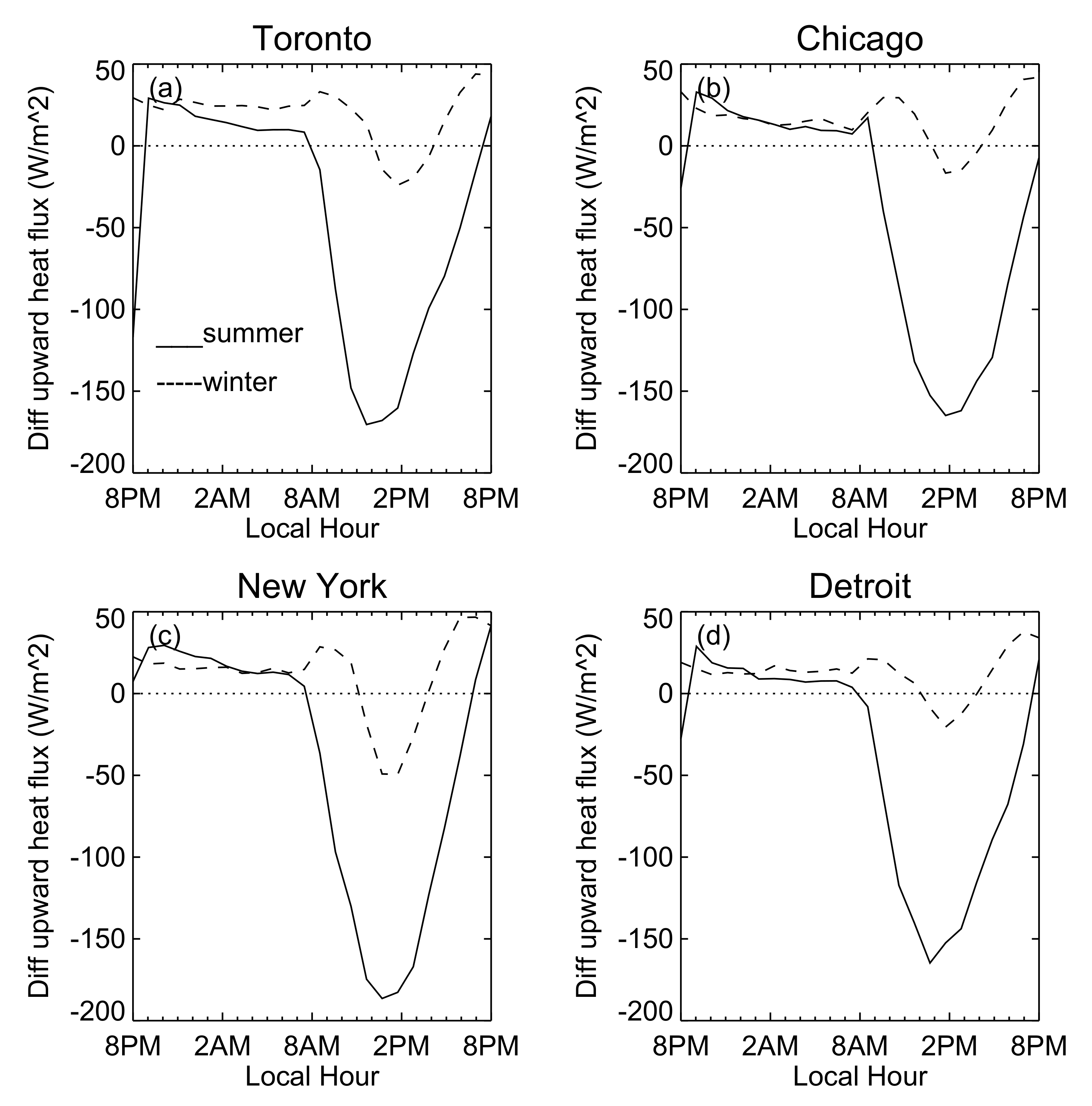
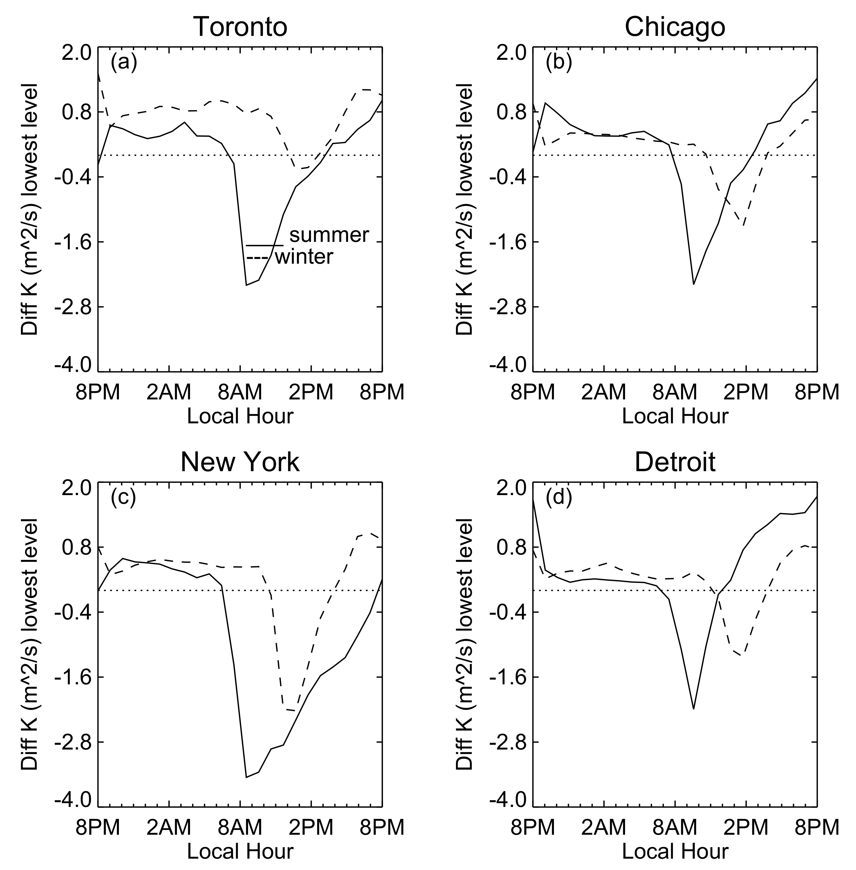
In order to examine the impact of the TEB scheme on the vertical diffusivity, monthly mean diurnal variations of
K differences between the TEB and non-TEB simulations are computed. The differences at the lowest model level (24 m above the ground) over the four urban centers in July and January are shown in
Figure 5. The figure shows that in July, the diurnal variation patterns and magnitudes of the differences over the four urban centers are similar with a negative value (between 7:00 a.m. to 4:00 p.m.) during the daytime peaking at 8:00 a.m. and a positive value in the early morning and at nighttime. Among the four urban centers, New York City has the largest differences during the daytime due to big surface heat flux reduction (
Figure 4). In January, the diurnal variation patterns over the four centers are similar. However, the magnitudes of the differences over the three U.S. urban centers are very different from that over Toronto. The former ones are just half of the latter in the early morning and at nighttime, but much larger magnitudes during the daytime. In addition, the negative differences over the three U.S. urban centers last much longer.
The comparison of the diffusion coefficient differences between summer and winter suggests that the reductions of
K by urbanization in summer and winter are different in both magnitude and variation pattern. In summer, the magnitude of the reduction over the four urban centers during the daytime is about 2 m
/s which is larger than 1 m
/s in winter over the three U.S. urban centers, and much larger than 0.2 m
/s over Toronto. Furthermore, the maximum reduction occurs around 8:00 a.m. in summer which is much earlier than 12:00 a.m. in winter. In addition to the differences during the daytime,
K enhancement in the early morning and at nighttime over Toronto is twice as much as that in summer. All these differences are due to the very different diurnal variation pattern and magnitude of the heat flux difference between summer and winter shown in
Figure 4.
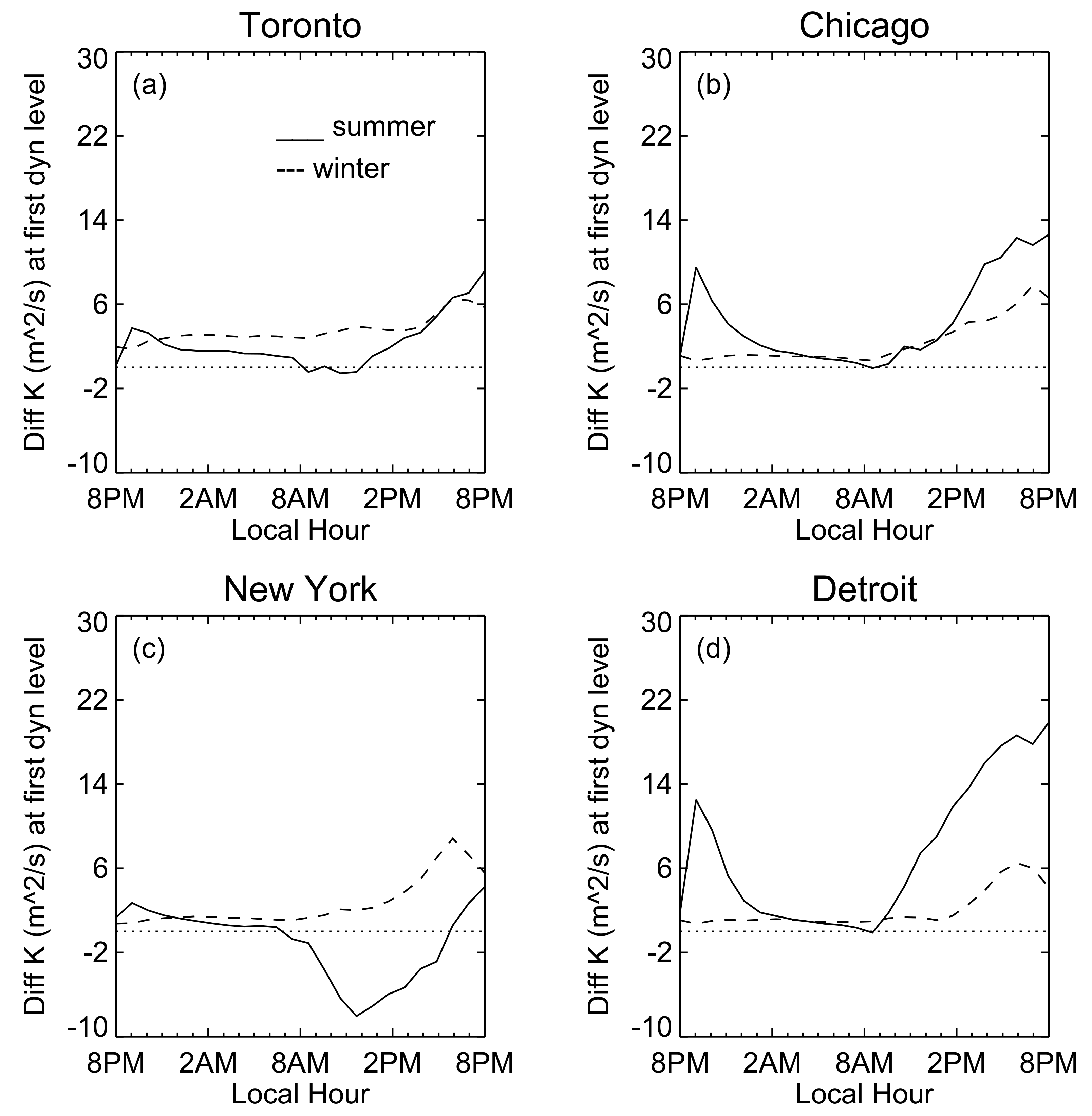
In GEM-MACH,
K at the lowest momentum level (about half level above the lowest model level) is used to compute the time tendency of temperature and chemical species at the lowest model level. Therefore the
K differences at this model level need to be examined. The monthly mean diurnal variation of this difference over the four urban centers is presented in
Figure 6. The comparison between
Figure 5 and
Figure 6 shows that the differences at the two levels are very different. While the winter differences have negative values during the daytime at the lowest model level, they are positive over 24 h at the lowest momentum level. In summer, the differences have negative values over the four urban centers at the lowest model level, they have big negative values only over new York City and extremely small negative values over Toronto. It will be shown that these features can help understand the sensitivity of concentration of chemical species to urbanization.
4.2. Impact On Temperature
The impact of the TEB scheme on urban temperature can be measured at different height including the level within the canopy layer, at top of canopy layer and within the urban boundary layer (UBL0. The temperature differences at these levels are used to measure the canopy, surface and UBL UHI effects [
4]. In the following we will examine the temperature differences at the lowest model level and at at 1.5 m.
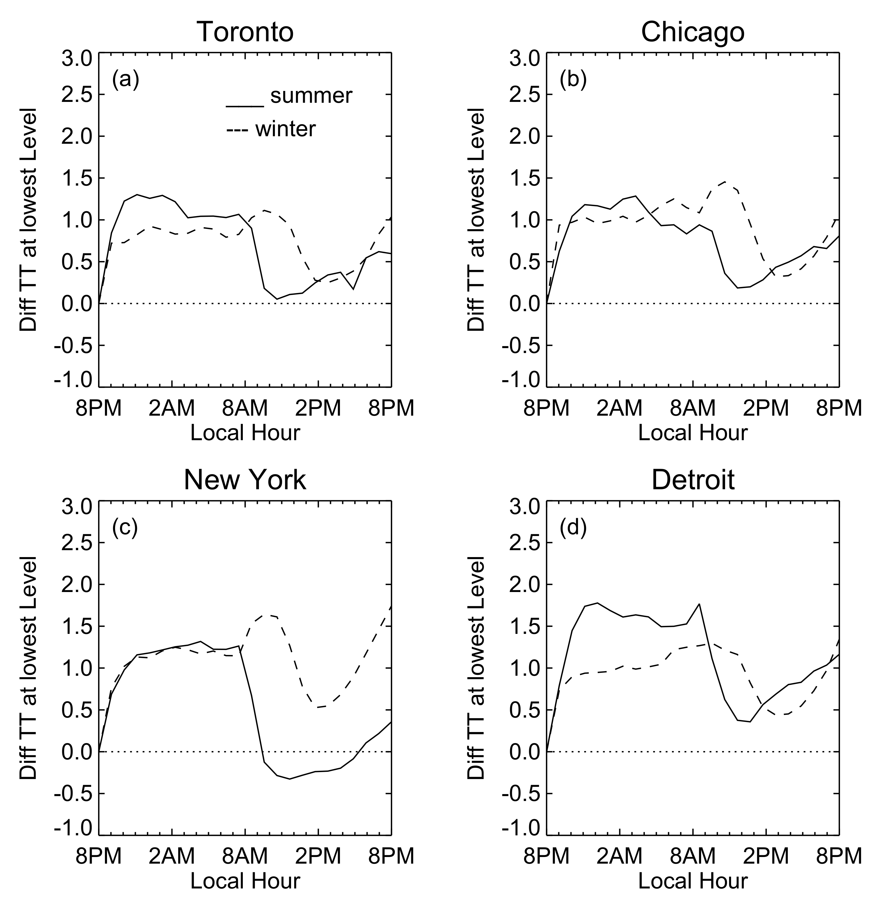
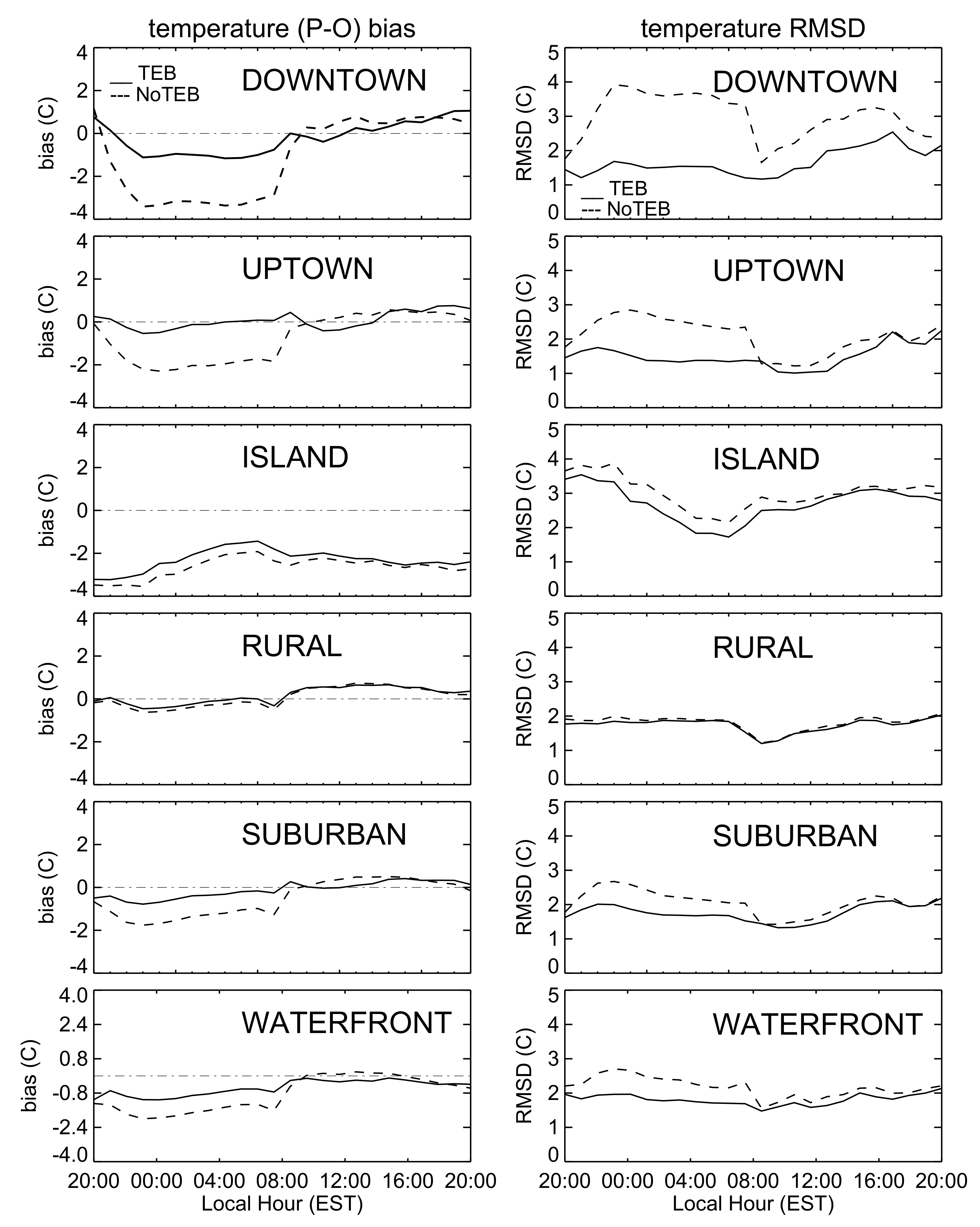
The monthly mean diurnal variations of the temperature differences between TEB and non-TEB simulations at the lowest model level are shown in
Figure 7. In the figure, about 1
C to 1.5
C temperature enhancement by the TEB scheme appears in the early morning until 8:00 a.m. and at nighttime over the four urban centers in both summer and winter. Corresponding to the reduction of surface heat flux, the temperature difference drops quickly from 8:00 a.m. until 10:00 a.m. in summer and 12:00 a.m. in winter, and then gradually decreases. The difference remains positive over the four urban centers in winter and also in summer except over New York City where the temperature difference is negative between 8:00 a.m. and 4:00 p.m. The positive temperature differences during the daytime suggest that urbanization can lead to the UHI effect not only in the early morning and at nighttime, but also during the daytime when the urban surface heat fluxes are reduced by the TEB scheme (
Figure 4). The comparison of the summer and winter cases suggests that in the early morning and at nighttime the UHI effect is stronger in summer than in winter, but weaker during the daytime except over the urban center of Detroit.
Due to the use of the same initial and lateral and upper boundary conditions, absence of direct feedback of chemistry to solar radiation in GEM-MACH and negligible humidity differences above 400 m, the incoming solar radiation at the lowest model level is the same in the TEB and non-TEB simulations. Thus urbanization affects urban temperature by changing the surface heat flux, vertical mixing and wind. Because the temperature difference between the two adjacent model grids (2.5-km) is less than 0.2
C, and the change of wind speed by the TEB scheme is about 0.4 (m/s) in average (see
Section 4.3.1), the change of the temperature advection over one hour due to the wind change is very small (0.08
C) The contributions of the changes in surface heat flux and diffusivity are discussed in the following part.
In order to understand the mechanism underlying the impact of the change of surface heat fluxes and vertical mixing on urban temperature, Ren and Stroud [
35] employed a theoretical model to show explicitly how the changes in urban surface flux and vertical diffusivity as well as the reference state affect urban temperature. In a semi-infinite domain, the analytical solution with a time-varying
, where
T is a dimensionless variable, to the simple model shows that the temperature response
to the change of surface heat fluxes and vertical mixing can be described by the following equation
where
.
and
are the differences of diffusion coefficient and surface heat fluxes between the TEB and non-TEB simulations shown in
Figure 5 and
Figure 7, respectively. Equation (
2) shows that the Green function (
G) decreases as height increases, and is small/big when diffusivity is weak/strong in general. The work of Ren and Stroud shows that
is negative below 80 m.
The temperature differences shown in
Figure 7 are produced by the combined effects of
and
. Ren and Craig examine the contribution of each effect based on Equation (
1) with the typical values of
,
and
K. The results show that because
is positive in the early morning and at nighttime, and the vertical gradient of the reference temperature is also positive due to temperature reversion, the enhanced
by the TEB scheme leads to warm effect. However, the temperature enhancement by
is about 0.2
C due to weak temperature difference between the lowest model level and the level above. The temperature increments produced by positive
during the period have similar magnitude to that shown in
Figure 7. Therefore,
is the dominant contributor to the UHI phenomenon. The results also show that the impact of
on
is also small during the daytime.
The small impact can be also understood by examining the temperature differences between the noontime and 16:00 p.m. During this period,
at the lowest momentum level is positive except over New York City and increases quickly in both summer and winter. According to Equation (
1), the positive
would lead to temperature decrease because the gradients of
and
G are negative. However the temperature differences during this period increase rather than decrease as
increases. This suggests that
is a dominant contributor to the variation of
during the daytime.
According to Equation (
1) the impact of
on urban temperature is modulated by
G. This modulation effect can be applied to explain the different temperature response in the early morning and during the daytime in summer. Equation (
1) shows that the drop of
during the daytime from its value in the early morning is a consequence of reduction of
. Although the magnitude of the surface heat flux reduction during the daytime in summer is about seven times larger than the magnitude of heat flux enhancement during the early morning and nighttime (
Figure 4), the corresponding temperature drop shown in
Figure 7 has the same magnitude as that of temperature enhancement. Because the diffusivity during the daytime is about 20 times larger than the diffusivity in the early morning, the strong diffusivity would damp the impact of
through
G according to Equation (
1), and this explains the disproportionate temperature response to the surface heat flux changes during the daytime.
The modulation effect on the impact of
on
through
G can be also applied to explain the different temperature responses to the surface heat flux changes in summer and winter. Although
Figure 5 shows that in the early morning, the surface heat flux enhancements in the downtown areas of Toronto and Detroit, are stronger in winter, the corresponding temperature enhancements shown in
Figure 7, however, are about 0.5
C lower. According to Equation (
1), the weaker temperature responses are due to a stronger diffusivity in winter (not shown). During the daytime, the surface heat flux reductions by the TEB scheme are about seven times stronger in summer than those in winter. Furthermore, the corresponding temperature drops in winter and summer are similar over the downtown areas of Toronto, Chicago and Detroit, and have about 1
C difference over New York City. The strong damping effect by
G associated with strong diffusivity in summer is responsible for the weaker temperature responses.
Equation (
1) shows that the temperature response to
is the convolution of
and
. This suggests that the positive temperature response in the early morning can impact the temperature response during the daytime. This impact and the strong damping effect by diffusivity explain the positive
in winter over the four urban centers and in summer over the three urban centers during the daytime when
is negative.
The fact that the temperature at a given time is the convolution of
and
can be also employed to understand the different evolution pattern of temperature (
Figure 7) and heat flux differences (
Figure 5). While
Figure 4 shows that corresponding to the diurnal variation of radiation, the evolution patters of heat flux differences are nearly symmetric around noontime, such symmetry, however, does not exist in the diurnal variation of temperature differences in summer. The variation of the temperature is much slower in the afternoon than in the morning. The convolution of
and
destroys such symmetry even though the evolution of diffusion coefficient is symmetric around noontime.
In GEM, the lowest model level over downtown Toronto is at around 24 m, and the temperature at the screen-level (1.5 m) is calculated diagnostically. The impact of the TEB scheme on the temperature at this level has similar diurnal variation pattern as that at the lowest model level but with larger magnitudes (2.5 C).
The impact of urbanization on temperature is not limited to the lowest model level, and the variation of the impact with height is discussed in
Section S2.
4.2.1. Impact on Humidity
In the TEB scheme, the impact of roofs and roads on urban hydrology is considered in the evolution equation of water-reservoir [
21], and the turbulent fluxes of heat and humidity are calculated in a similar way. Due to the small impact of the change of wind, the urbanization affects the urban humidity through surface heat flux and the vertical mixing. Because the surface of urban components in the TEB scheme is impervious and the liquid precipitation intercepted by roads and roofs goes into underground sewer systems, the surface humidity fluxes in the TEB simulation should be much weaker than that in the non-TEB simulation in urban areas.
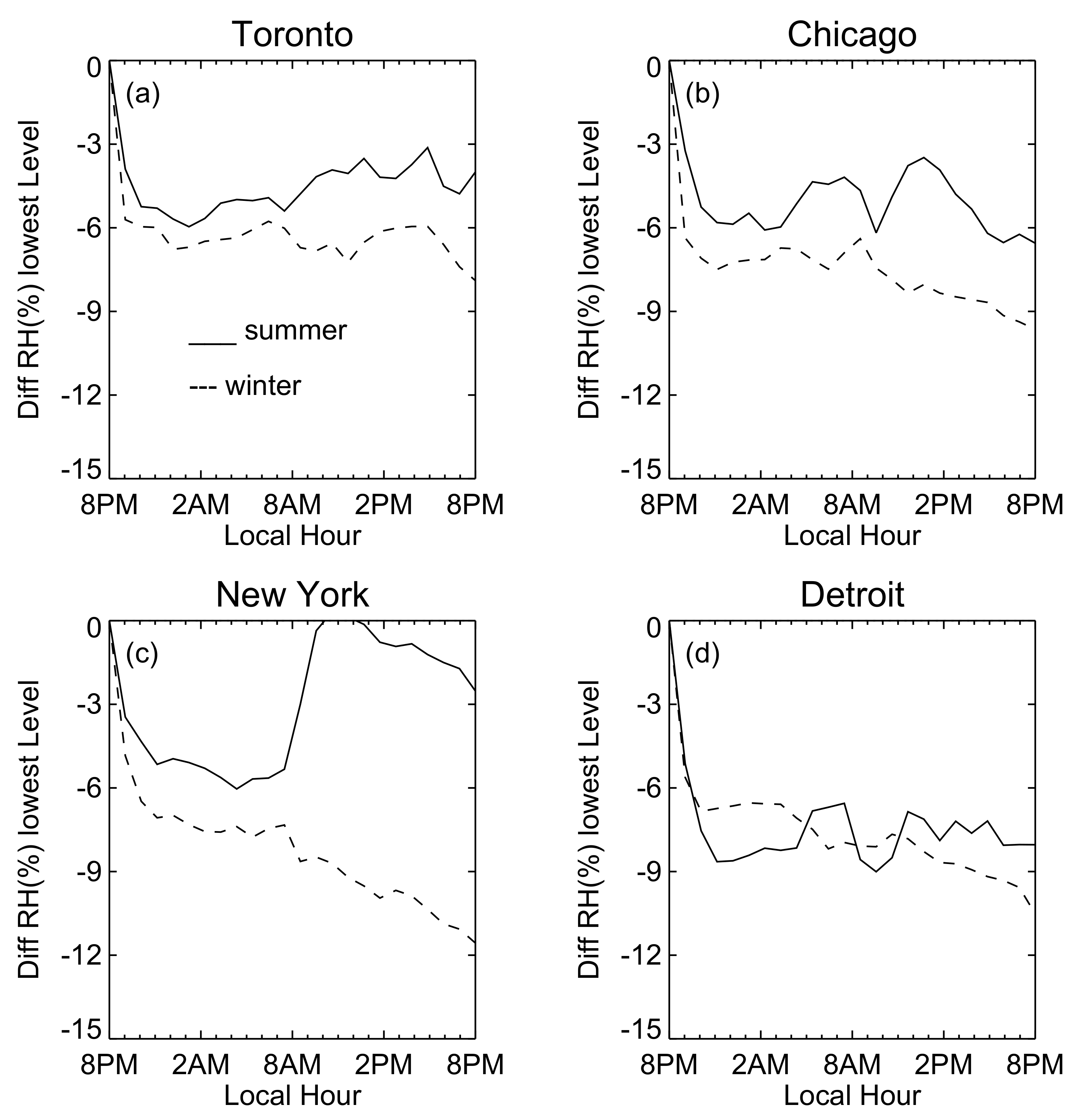
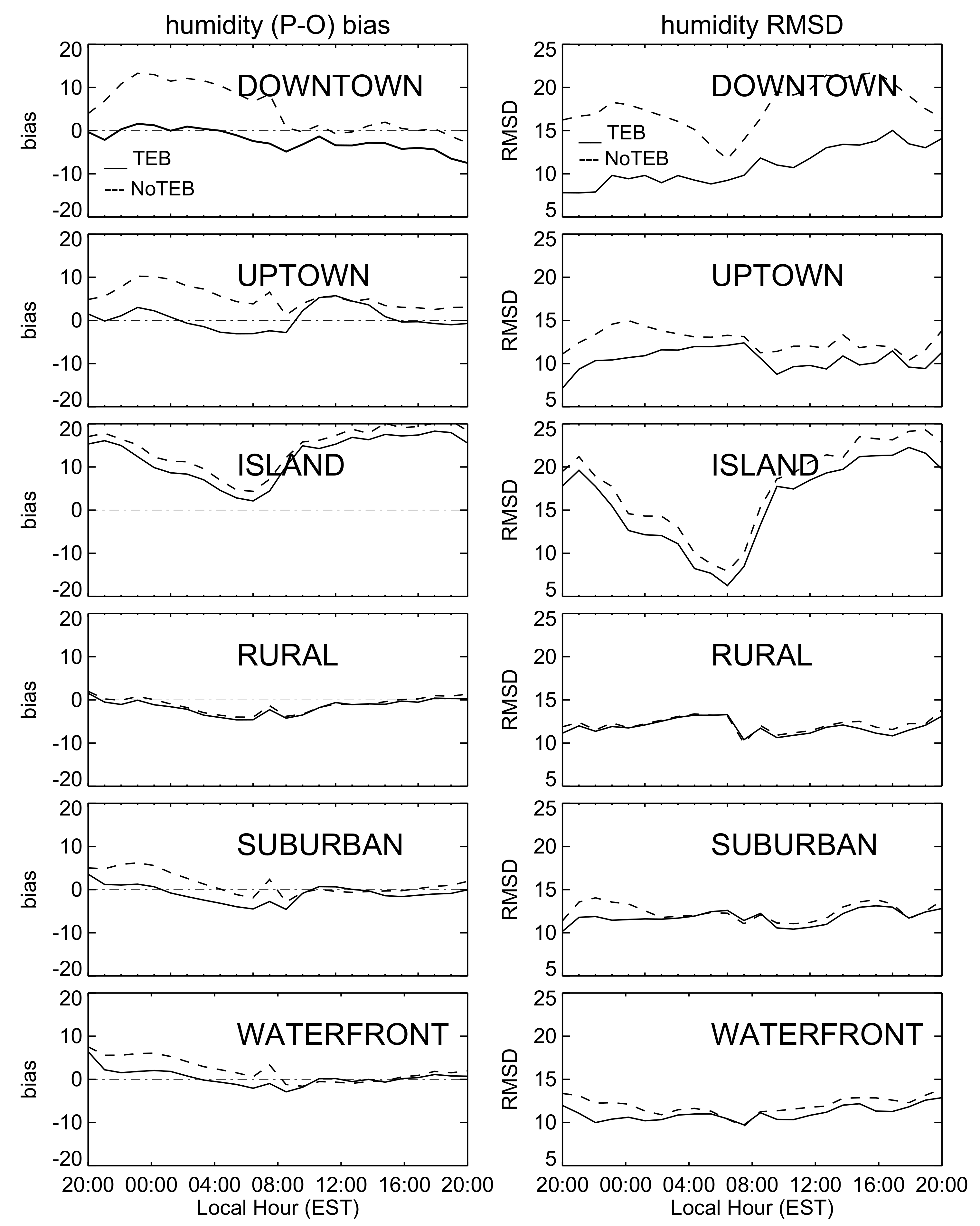
In order to examine the impact of the TEB scheme on humidity, the diurnal variations of the monthly mean urban relative humidity difference over the four urban centers are computed, and the differences at the lowest model level are presented in
Figure 8. It can be seen from the figure that urbanization leads to the reductions of humidity in both summer and winter, and the reduction is larger in winter than in summer. The variation of the differences in summer is smooth except over New York City. In winter, the TEB scheme leads to continuous drop of relative humidity except over Toronto. The impact on humidity can lead to not only the change of latent heat flux, but also changes in the uptake of water onto hydroscopic particles, as well as chemical reactions such as
.
Specific humidity is another variable measuring the humidity level in the atmosphere. Comparison between the TEB and non-TEB simulations shows that the TEB scheme also leads to the reduction of specific humidity over the four urban centers. In winter, the reduction at the lowest model level is about 2% of the specific humidity in the non-TEB simulation between 8:00 p.m. to 8:00 a.m. over the four urban centers, and 14% over New York, 7% over other centers between 10:00 a.m. to 7:00 p.m. In summer, the reduction is also about 2% of the specific humidity in the non-TEB simulation between 8:00 p.m. to 8:00 a.m. over the four centers, and is about 3% over New York, 6% over Toronto, and 10% over Chicago and Detroit. The TEB impacts on relative humidity and specific humidity decay rapidly with height, and they become negligible above 400 m.
4.2.2. Impact on the ABL Height
Because the top of the ABL separates the boundary layer and free troposphere, the ABL height describes the vertical extent of mixing process generated within the ABL, and thus imposes constraints on the exchange of momentum, energy and chemical species between the ABL and free atmosphere [
48]. Studies show that the ABL height has a strong negative correlation with air pollution in big cities [
49,
50]. In GEM-MACH, the ABL height is involved in the TKE scheme through
in the surface boundary condition in the unstable case [
47]. It is also utilized in two places: in the calculation of the plume-rise height for anthropogenic major point source emissions and forest fire emissions, and in assigning the minimum of diffusion coefficient within the ABL.
In numerical models, the ABL height is not a prognostic variable. Different methods have been used to calculate the ABL height, and each method produces quite different results [
51]. Among these methods, potential temperature (PT)-based method and the Richardson number (R
)-based methods are two popular methods. Because the PT-based method is used to compute the ABL height in GEM-MACH, the differences in vertical temperature profiles between the TEB and non-TEB simulations suggest that the TEB model would have a great impact on the ABL height.
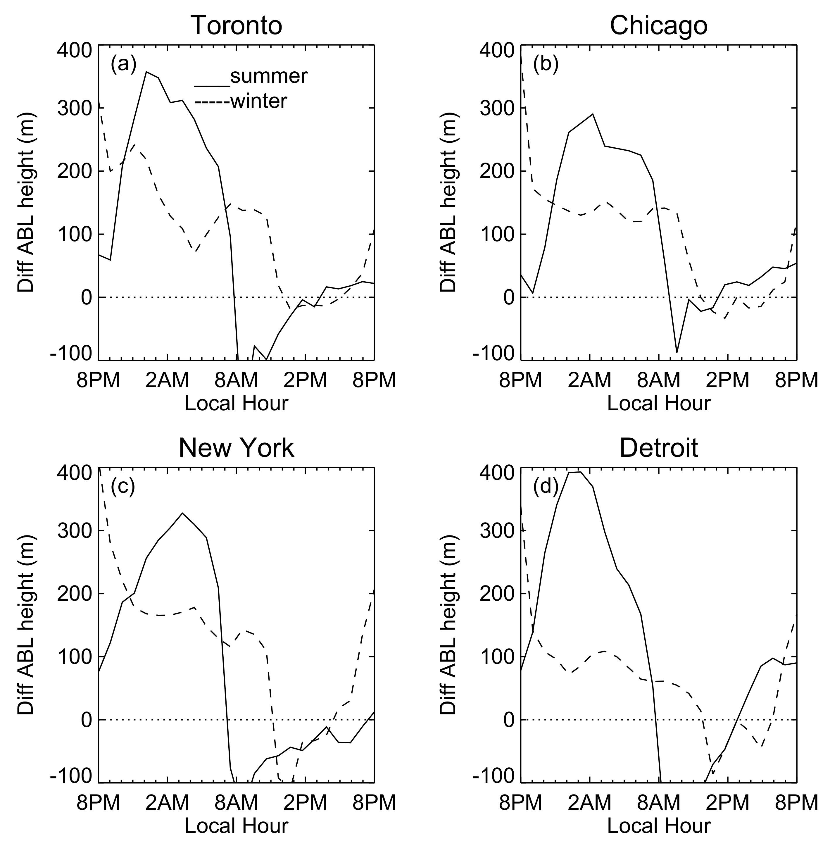
The monthly mean diurnal variations of the ABL height differences between the TEB and non-TEB simulations are shown in
Figure 9. It can be seen from the figure that the TEB scheme has similar impact on the ABL height in summer over the four urban centers. Large positive difference drops rapidly from 2:00 a.m. and becomes negative around 8:00 a.m. It then starts to increase until 4:00 p.m. and has very small changes between 4:00 p.m. and 8:00 p.m. Rapid increase occurs between 8:00 p.m. and 2:00 a.m.
The diurnal variations of the differences in winter are different from those in summer. The positive differences in the early morning are much smaller and variations are much slower than those in summer. Rapid drops occur at around 8:00 a.m. and continue until noontime. The drops are much deeper over New York City and Detroit than over Toronto and Chicago. While the differences over New York City and Detroit start to increase quickly after noontime and reach maximum value around 7:00 p.m., they remain around zero over Toronto and Chicago until 4:00 p.m. The enhancement of the ABL height in the late afternoon by the TEB scheme is much larger in winter than in summer.
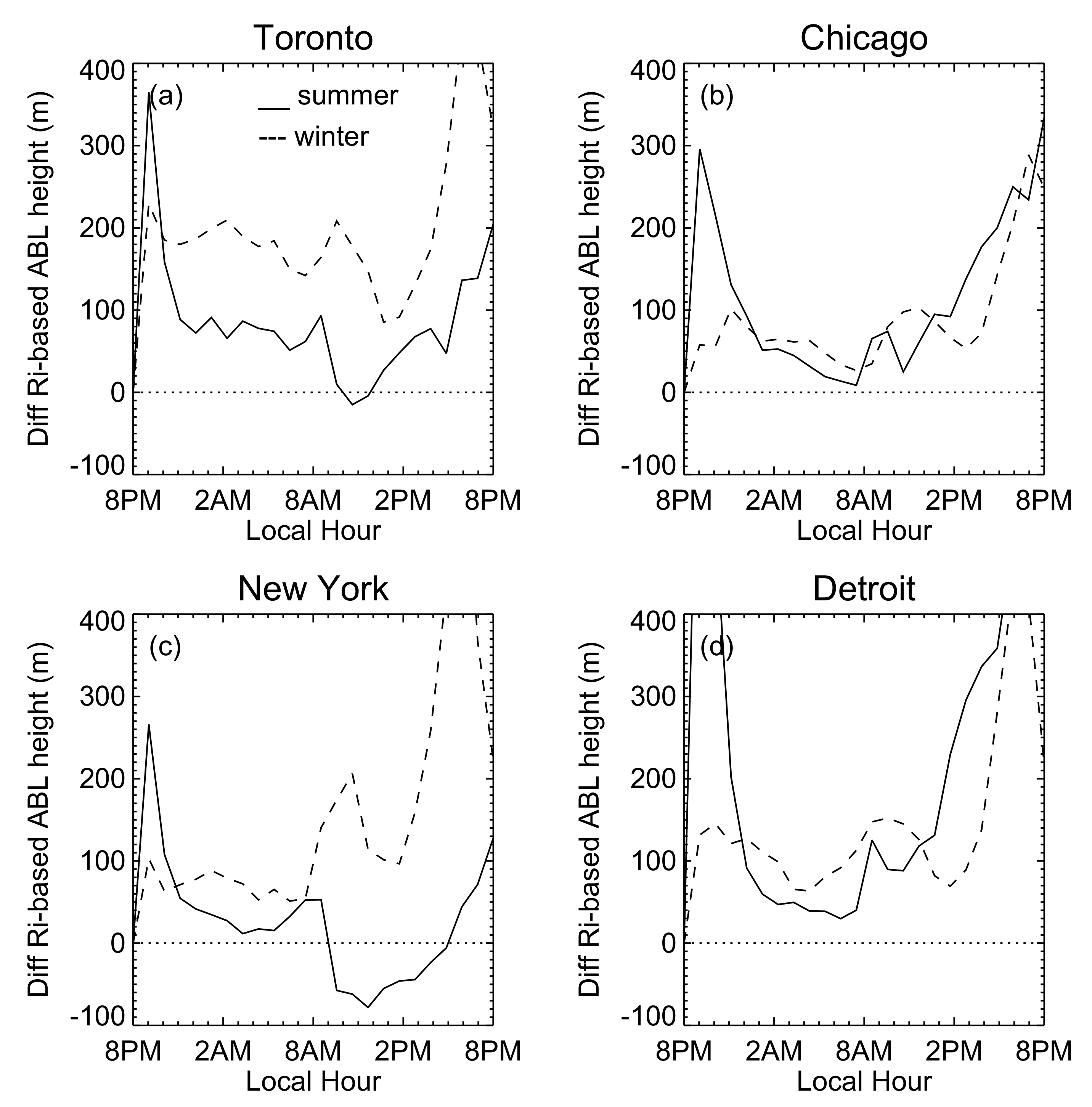
To show the sensitivity of the ABL height calculated using the
-based method, ABL height differences based on this method are computed offline, and their diurnal variations are shown in
Figure 10. In the figure, the differences are zero at 8:00 p.m. due to re-initialization. The figure shows that in summer, the differences are quite similar between 4:00 p.m. to 8:00 a.m. over the four urban areas. During this period, the TEB scheme leads to the ABL height enhancement. The enhancements increase rapidly from 4:00 p.m. until 10:00 p.m., then drop quickly between 10:00 p.m. and 11:00 p.m. They continue to drop after 11:00 p.m. but with a much slower rate until 7:00 a.m. and then increase slightly until 8:00 a.m. Between 8:00 a.m. and 4:00 p.m. the difference over New York City is different from those over the other three urban areas. During this period, while the TEB scheme leads to as much as 100 m reduction over New York City, but small enhancement in other three urban areas (except a small reduction around 9:00 a.m. over Toronto). In winter, the TEB scheme leads to the enhancement of the ABL height over the whole day over the four urban centers. The differences over the four areas are very similar with a large enhancement in the afternoon. The evolution patterns between 1:00 a.m. and 6:00 p.m. are similar to those in summer except over New York City.
The comparison between
Figure 9 and
Figure 10 suggests that the sensitivities of the ABL height based on the two approaches are quite different. In summer, while the large PT-based ABL height enhancements appear in the early morning, and large reductions appear in the morning over the four urban areas, the large R
-based enhancements appear at the nighttime, and large reductions appear only over New York City. In winter, while the large PT-based ABL height enhancements appear between 8:00 p.m. to 10:00 p.m., and reductions appear in the early afternoon over the four urban areas, the large R
-based enhancements appear in the late afternoon, and there is no reduction.
4.4. Impacts on Urban Pollutants and AQHI
Air pollutants have adverse effects on human health and cause damages on trees, vegetables and buildings. Their impacts are measured by the Air Quality Health index (AQHI) developed by the Environment and Climate Change Canada (
https://www.canada.ca/en/environment-climate-change/services/air-quality-health-index/, accessed on 10 February 2020). Due to high population density and high concentration of air pollutants in the urban areas, the impacts of urbanization on urban chemical environment have been widely studied. In the following part the impacts of the TEB scheme on the evolution of some major urban pollutants and AQHI are examined by comparing the TEB and non-TEB simulation results.
Several factors including boundary conditions, short-wave solar radiation and meteorological conditions can affect the regional model simulations of major air pollutants. In the TEB and non-TEB simulations, the same chemical and meteorological lateral and upper boundary conditions are used. Although the same surface emissions are used in TEB and non-TEB simulations, the dry deposition velocities can be different over urban areas due to different surface momentum flux. Therefore, surface chemical boundary conditions can be different in the two simulations. Due to the lack of direct feedback of chemistry to solar radiation and extremely small differences in humidity above 400 m, the incoming solar radiation should be roughly the same in the two simulations. However, the reflected solar radiations in the two simulations over urban areas can be different due to different albedo. Thus changes in meteorological fields, chemical boundary conditions at bottom, chemical reactions, and reflected solar radiations can lead to differences in the concentration of air pollutants between the two simulations. These differences are examined in this section.
4.4.1. Impact on Carbon Monoxide
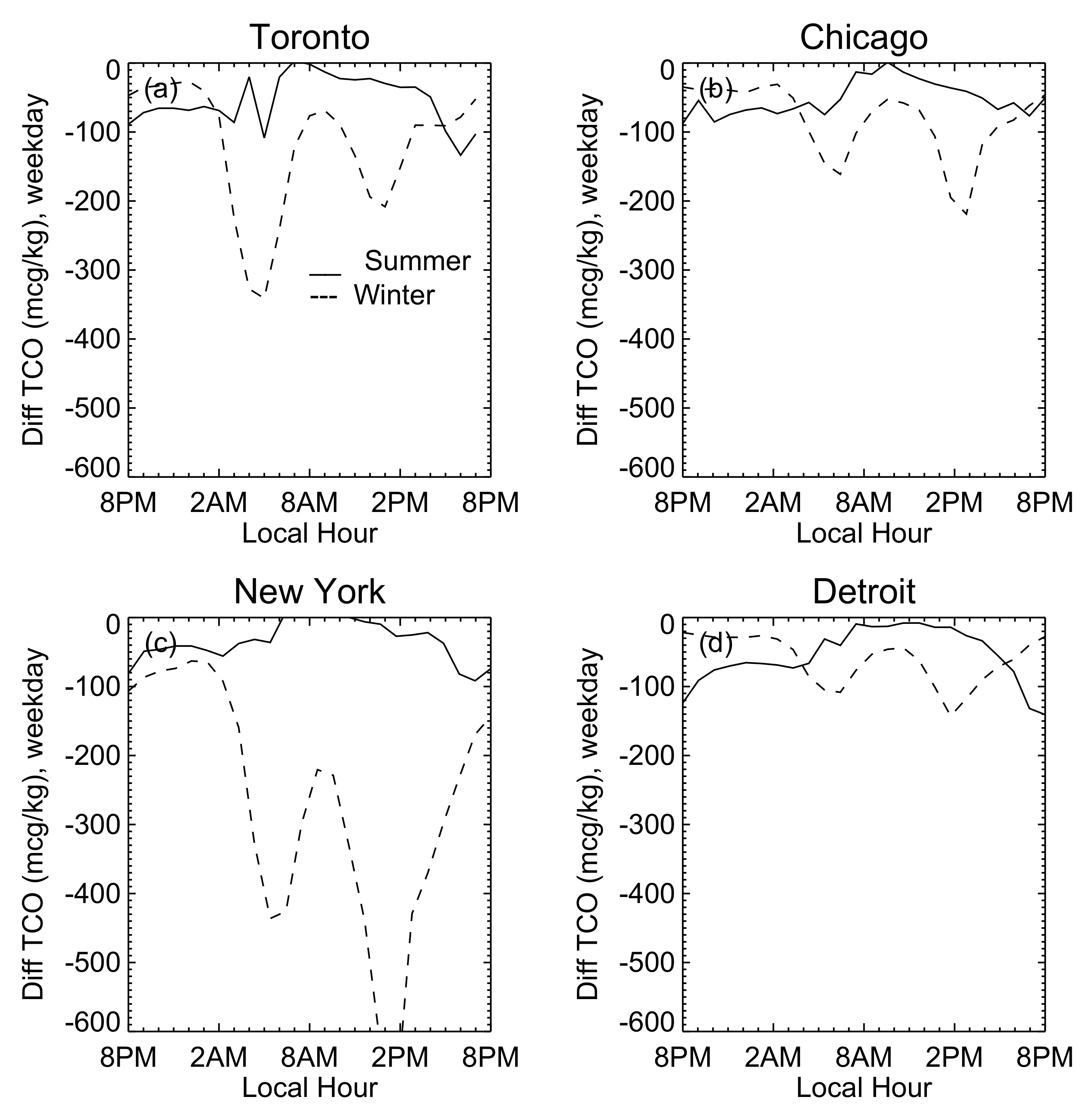
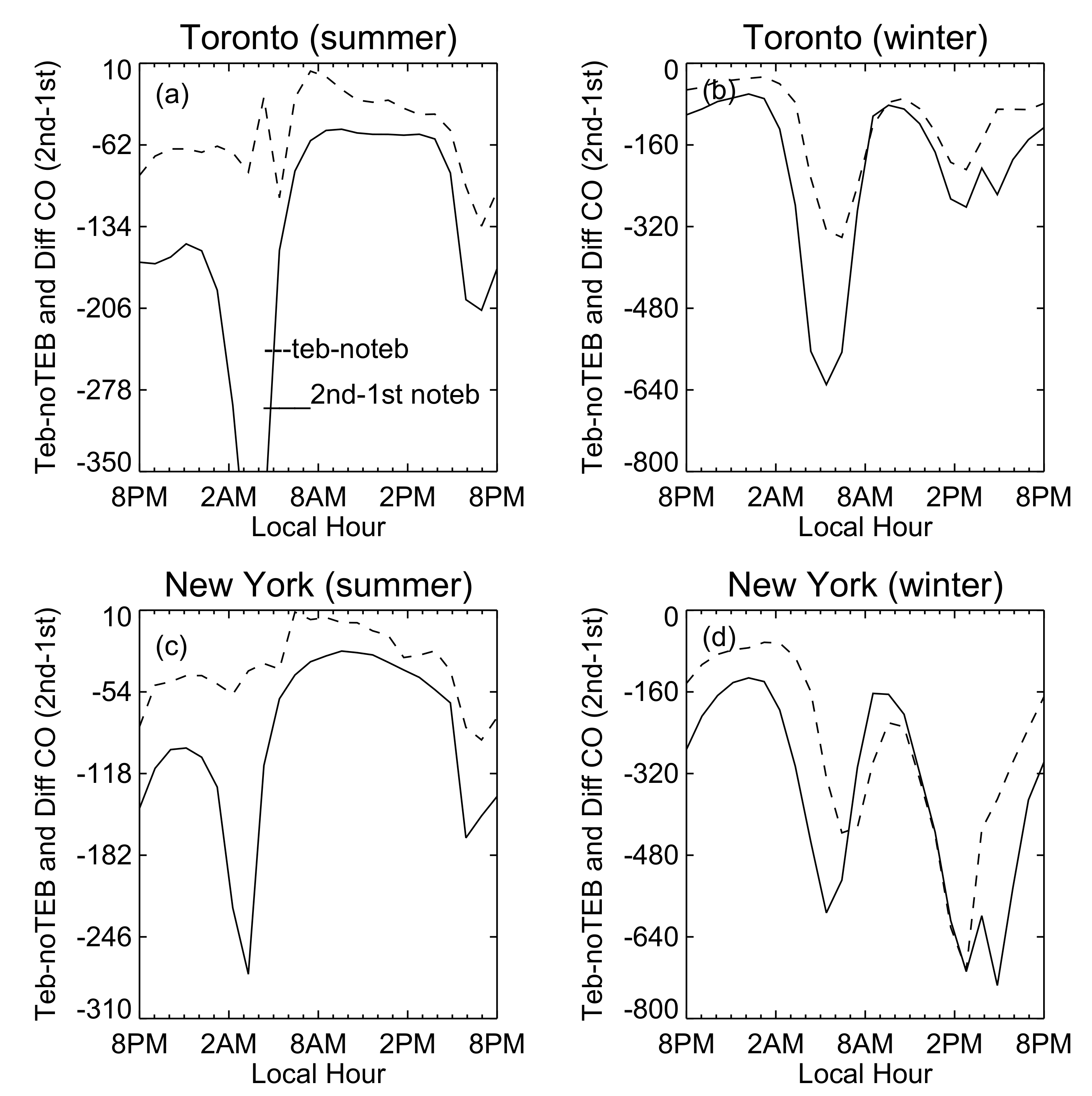
Among the major air pollutants, carbon monoxide (CO) can be taken as a passive tracer. The concentration differences between the TEB and non-TEB simulations can be attributed to the change of meteorological fields due to the TEB effects. The TEB impacts on the CO mixing ratio can be seen from
Figure 12 which shows the weekday mean diurnal variations of the mixing ratio differences between the TEB and non-TEB simulations. The figure shows that in summer, the diurnal variation of CO mixing ratio differences over the four urban centers are quite similar. The TEB scheme leads to 50
g/kg mixing ratio decrease in the early morning and 100
g/kg (about 28%) decrease in the late afternoon. Between 8:00 a.m. and noontime, the TEB scheme has a small impact. In winter, the diurnal variation patterns of the differences are also similar over the four urban centers with two drops of the differences: one in the early morning between 0:00 a.m. and 4:00 a.m. and another at around noontime. However, the magnitudes of the two drops are very different over different urban centers. Over New York City, the first drop is more than 400
g/kg (25%), four times larger than that over Detroit, and the second drop is about 600
g/kg (50%), which is five times larger that over Detroit.
The figure also shows that the TEB has very different impacts in summer and winter. In summer, the differences over the four urban centers vary slowly in the early morning, but vary rapidly in winter, especially over Toronto and New York City. During the daytime, big difference appears in the late afternoon in summer, but appears around 1:00 p.m. in winter. Overall, the TEB scheme leads to much larger mixing ratio decrease in winter time than in summer time.
The changes of both wind and vertical mixing by the TEB scheme can contribute to the mixing ratio difference shown in
Figure 12. Although their contributions cannot be separated, the contribution of the changes in wind can be assessed based on the magnitude of
, where
is the horizontal gradient of mixing ratio. Because the magnitude of this term is less than 30
g/kg/h in the early morning over Toronto and New York City, it cannot account for 100
g/kg/h drops. Therefore the contribution associated with the change of vertical mixing is dominant.
Because the impact of diffusivity on tracer concentration can also be described by the 1-D diffusion model, Equation (
1) can be applied to interpret the numerical results shown in
Figure 12. Because the same boundary and initial conditions are used in the TEB and non-TEB simulations, the differences in mixing ratios between the two simulations in the 1-D model can be written as
Unlike the temperature gradient which is positive in the early morning, the gradient of the CO concentration is always negative. Thus according to Equation (
4), positive/negative
at the lowest momentum level would lead to the decrease/increase of mixing ratio (because the gradient of
G is negative). Comparison between
Figure 6 and
Figure 12 suggests that it is indeed the case. Positive
in winter corresponds to negative
over the four urban areas over 23 h. In summer, positive
also corresponds to negative
. Furthermore, the negative
between 8:00 a.m. and 12:00 a.m. in summer over New York City and Toronto corresponds to (small) positive
.
According to Equation (
4), the impact of change of vertical diffusivity on tracers is modulated by the vertical gradients of mixing ratio of the non-TEB simulation and
G. For a given
, large/small magnitude of the vertical gradients of
and
G would enhance/weaken the impact. To examine the modulation effects, CO mixing ratio difference between the lowest model level and one level above in the non-TEB simulation (
) is used to represent the vertical gradient of mixing ratio. Because the TEB scheme has a larger impact on mixing ratio over urban centers of New York City and Toronto, the diurnal variations of (
) over the two urban centers are presented in
Figure 13 along with the mixing ratio differences between the TEB and non-TEB simulations (
) at the lowest model level. It can be seen from the figure that except in the early morning in summer, the diurnal variation patterns of
and
are quite similar. The correlation between
and
is more robust in the afternoon than in the morning due to larger
, and the correlation in winter is more robust than in summer.
The modulation of the vertical gradient of
G can be identified by comparing the variation of
during the daytime in summer. According to Equation (
4) the negative
shown in
Figure 6 over New York City and Toronto between 8:00 a.m. and 12:00 a.m. in summer would enhance mixing ratio. Although the magnitude of
over New York City is much larger than that in Toronto, the enhancements over the two urban centers are quite similar (
Figure 12). Because the values of
over the two centers are similar, the similar mixing ratio enhancements should be due to a weaker vertical gradient of
G. This weaker gradient is caused by a stronger diffusivity over New York City which is much stronger than the diffusivity over Toronto. The numerical results show that the TEB scheme has similar impacts on PM
.
4.4.2. Impact on NO, NO and O(g)
Because NO
and O
(g) are involved in photochemical reactions, they cannot be taken as a passive tracers. Thus both
and the change of chemical reactions due to the change of mixing ratio by
can affect the mixing ratio of the two species. Their impacts can be seen in
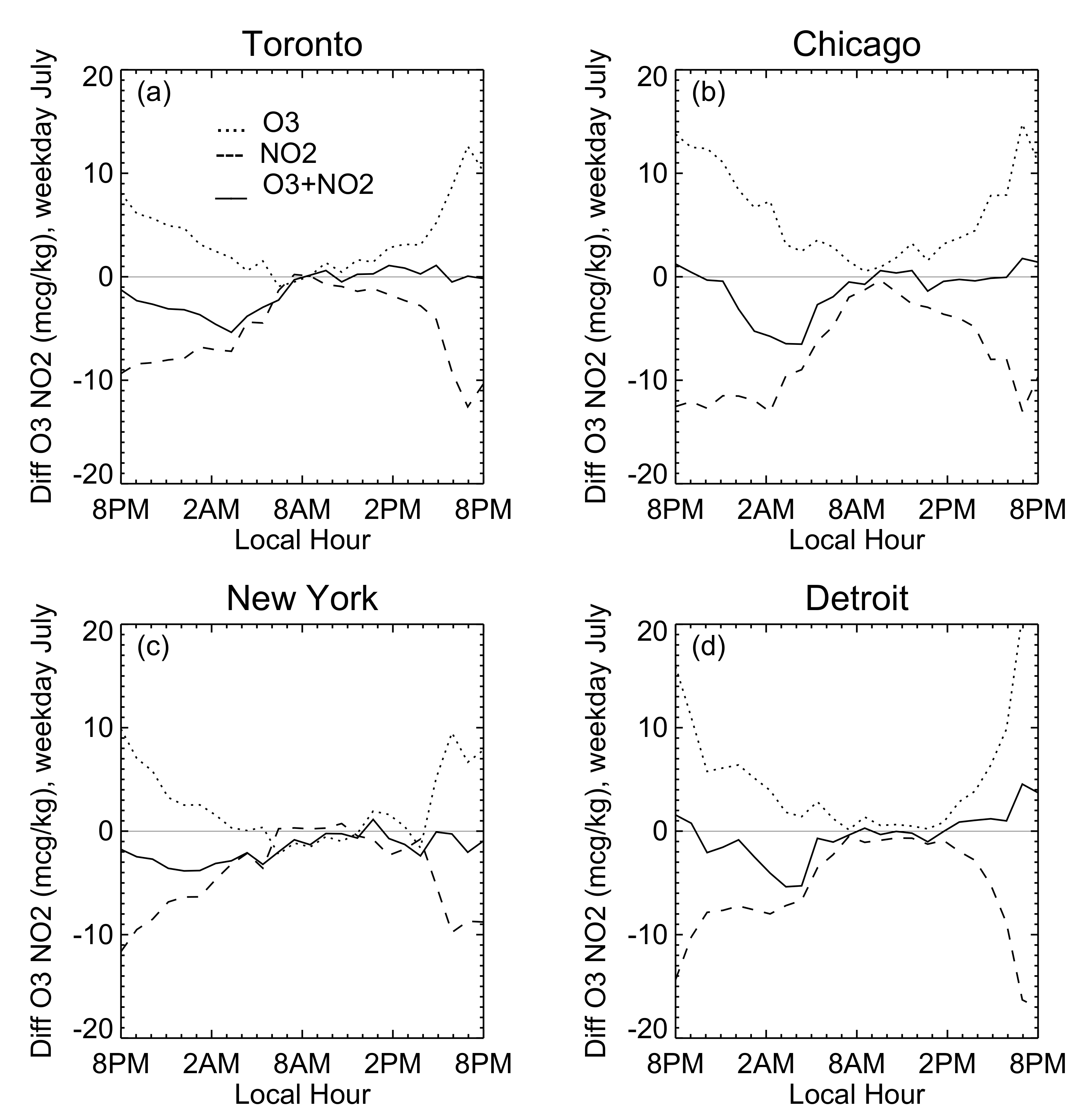
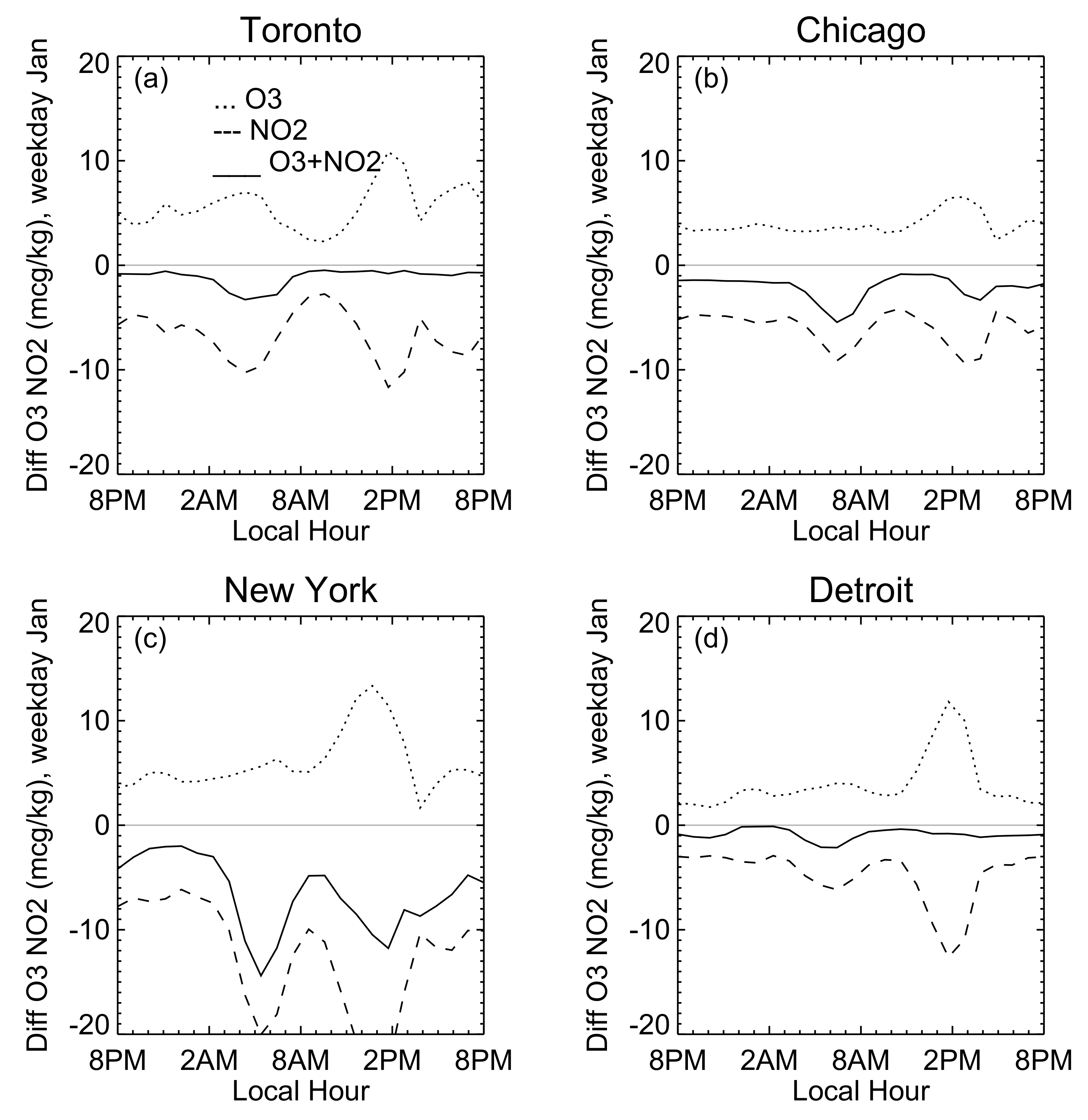
Figure 14 which shows the diurnal variations of the weekday mean NO
mixing ratio differences (
) in summer and winter. The comparison between this figure and
Figure 12 suggests that the evolution patterns of the mixing ratio differences of CO and NO
are quite similar over the four urban centers, suggesting that
plays a major role in affecting the mixing ratio. Numerical results also show that in summer the variation of mixing ratio of NO
correlates closely with the vertical gradient except in the early morning (between 0:00 a.m. to 2:00 a.m.). In winter, strong positive correlation can be identified except between 1:00 p.m. and 6:00 p.m. over Toronto and between noontime and 4:00 p.m. over New York City during which the correlations are negative (not shown).
O
(g) is produced by the photochemical reactions of nitrogen oxides (NO
) and volatile organic components (VOCs) during the daytime, and is destructed by reacting with NO to form NO
. Therefore the diurnal variation of O
(g) difference (
) should be opposite to the variation of the NO
(summation of NO and NO
) difference as shown in
Figure 15. In summer, the variations of the O
(g) differences correlates negatively with the variations of the NO
difference. However, the magnitudes of the two differences are different. In the early morning, the magnitude of NO
can be 10
g/kg more than that of
, and about 5
g/kg at nighttime. In winter, however, the magnitudes of
are much smaller than those of
except in the afternoon over urban center of Detroit, and
has no response to the strong variation of
in the morning and at nighttime. Numerical results show that the modulations of
and
to
and
are similar to the modulation of
to
.
4.4.3. Impact on AQHI
AQHI is a scale designed by ECCC and Health Canada to measure the health impact of short-term exposure to air pollution. The concentrations of three major pollutants including ground-level ozone,
and
are used to calculate AQHI through the following formula
Because the value of AQHI increases exponentially with the increase of the concentrations of the three pollutants, high value of AQHI means great health risk associated with the air quality. Because AQHI is a nonlinear function of the concentrations of the three pollutants, the monthly mean difference of AQHI is not the linear combination of the monthly mean differences of the three pollutants.
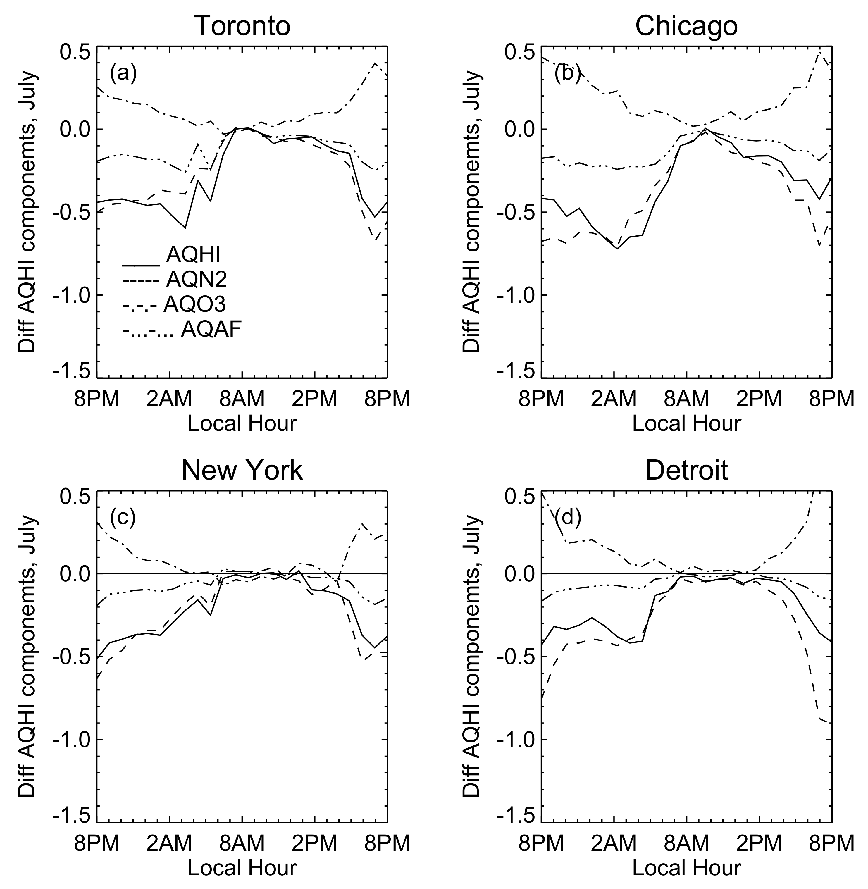
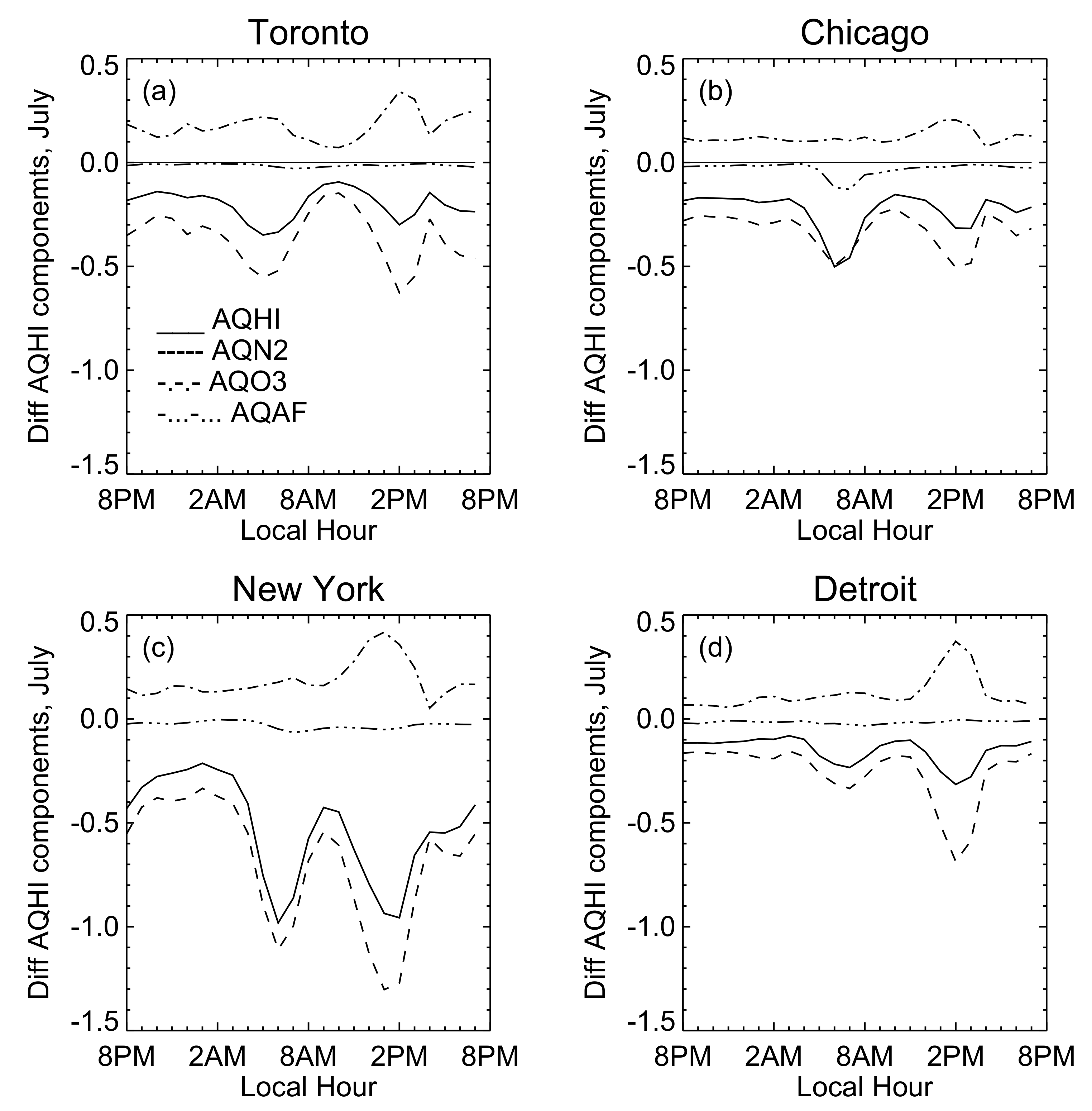
To show the impact of the TEB scheme on AQHI, monthly mean hourly AQHIs in July and January are computed, and the weekday mean diurnal variations of AQHI and its components (AQ
, AQ
and AQ
) are presented in
Figure 16 and
Figure 17 for July and January, respectively. It can be seen from the two figures that while the TEB effect leads to the reduction of AQHI in summer between late afternoon and early morning in summer, it leads to the reduction in the whole day in winter. The impacts of the TEB scheme on AQHI are stronger in summer than in winter except over New York City where the reduction of AQHI can be as big as 1. The impacts are similar over the four urban centers in summer. and over Toronto, Chicago and Detroit in winter.
It can been seen from
Figure 16 and
Figure 17 that in summer, the enhanced AQHI by O
(g) enhancement in the early morning and at nighttime is offset by the reduced AQHI by the reductions of PM
and NO
. In winter, the contribution of PM
is extremely small and the reduction of AQHI is entirely due to the contribution of the reduction of NO
. In both summer and winter, the reduction of
by the TEB scheme plays a dominant role in reducing AQHI.
The numerical results also show that the reduction of AQHI in summer is much larger in weekend than in weekdays between late afternoon and early morning, but it is smaller in winter during this period (not shown).

 ,
, 


