The R Language as a Tool for Biometeorological Research


Laboratory of General and Agricultural Meteorology, Agricultural University of Athens, Iera Odos 75, 11855 Athens, Greece
Atmosphere 2020, 11(7), 682; https://doi.org/10.3390/atmos11070682
Submission received: 11 June 2020
/
Revised: 24 June 2020
/
Accepted: 27 June 2020
/
Published: 28 June 2020
(This article belongs to the Special Issue Challenges in Applied Human Biometeorology)
Abstract
:R is an open-source programming language which gained a central place in the geosciences over the last two decades as the primary tool for research. Now, biometeorological research is driven by the diverse datasets related to the atmosphere and other biological agents (e.g., plants, animals and human beings) and the wide variety of software to handle and analyse them. The demand of the scientific community for the automation of analysis processes, data cleaning, results sharing, reproducibility and the capacity to handle big data brings a scripting language such as R in the foreground of the academic universe. This paper presents the advantages and the benefits of the R language for biometeorological and other atmospheric sciences’ research, providing an overview of its typical workflow. Moreover, we briefly present a group of useful and popular packages for biometeorological research and a road map for further scientific collaboration on the R basis. This paper could be a short introductory guide to the world of the R language for biometeorologists.
1. Introduction: The Biometeorology in the New Research Era
As Tromp (1963) [1] defined, biometeorology is “the impact of the weather and climate on humans and their environment (animals and plants)” giving a succinct and full description of this interdisciplinary science. The origins of this science’s branch lie in antiquity, but its vigorous growth only dates back to the years following World War II [2]. Ancient Chinese, Indians, and Greeks were studying the influence of weather on everyday activities, health, and wellbeing. The advances made by Hippocrates, Glisson, Benjamin Franklin, Huntington, de Ruder and Petersen identify the uninterrupted interest on the two-way interaction between the atmosphere and bio-environment [2,3,4]. Right after World War II, when computer power became more accessible and cheaper, a new wave of ideas and applications emerged. More complicated and accurate mathematical models coincided to describe human thermal biology and its interactions with the atmosphere. Höppe (1999) introduced the MEMI (Munich Energy balance Model for Individuals) model and the PET (Physiologically Equivalent Temperature) index, and Matzarakis, Lin, Nastos and many other scientists applied the new human energy budget index into urban and other complex environments [5,6,7,8,9,10,11,12,13,14]. Moreover, software applications such as RayMan, ENVI-met and UMEP gave further abilities to human biometeorology to provide solutions for landscape design, tourism, urban planning and so on [15,16,17,18]. Lastly, biometeorology covers a broad spectrum of topics, such as the interaction of the weather with animals, insects, pollution, working conditions, energy consumption, tourism and others [3,19,20,21,22].
Today, biometeorology evolves big data obtained by climate reanalysis processes, by thousands of meteorological stations on airborne, seaborne, or ground platforms, along with radar and lidar data. This adverse data enhanced with the emerging computational capacity and collaborative tools is the steam engine of the new era of research. The interdisciplinarity of these scientific branches requires new skills in order to achieve high quality research. The biometeorological research community sporadically takes advantage of the R language’s characteristics. Hence, we can find published papers in high reputation journals which are the outcome of R’s assisted analysis. Focusing mainly on the human biometeorological discipline, we can find papers dealing with health [23,24,25] or human behaviour [26,27] besides some core issues about the behaviour and calibration of thermal comfort indices and human thermal perception [28,29,30,31,32] along with the biometeorological conditions in urban or other complex environments [31,33,34,35,36,37,38]. The objective of the present article is the presentation of the research workflow linked and empowered by a data-analysis-oriented scripting R language. The main contribution of this paper is a brief guidance for the biometeorological research via R coding. Moreover, a grouped introduction of the most popular and useful R packages is presented for the implementation of a reproducible scientific workflow.
2. Methods and Tools in Biometeorology
2.1. The Classic Research Workflow
Interactions between weather or climate and the bio environment are complicated as a consequence of the spatiotemporal heterogeneity [39], and this complexity is mirrored by scientists’ research methodologies. As a community, we must answer clearly as to what we want, what we need and, finally, what we use for the purposes of our research. Hence, we want to handle big and varying data (factorial or numerical) from deferent sources (great variety of formats and structures) and to analyse and disseminate the results of the research. The community we want to interact with is far broader than the biometeorology academia. It consists of architects, landscape designers, physiologists, psychologists, biologists, climatologists and urban planners. We need tools for data acquisition and collection, for data organisation, for data modelling and, finally, for the dissemination of the results (presentation/communication). Generally, we use a stack of different software packages that drive us to excessive destruction and diaspora of our techniques and methodologies. This is a great leak of energy, a waste of time and a loss of valuable resources. The above common practice makes the automation and reproducibility of our science more laborious and sometimes impossible.
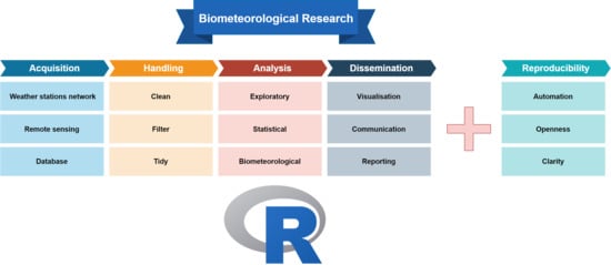
The following graph (Figure 1) is the classic or typical research workflow having 4+1 steps. The first step, as anticipated, is the data acquisition, followed by the data handling step. Then there is the analysis of the prepared data with the biometeorological methods. Finally, there is the step of results dissemination.
These are the four steps to conduct complete research. However, an important concern nowadays is the achievement of the reproducibility of our research. It is not a necessary step, but it boosts our research results’ reliability.
2.1.1. Data Acquisition
The first process of the research workflow is data acquisition. The adverse sources lead to a great variety of data file formats and structures. In order to obtain data, scientists are obliged to retrieve them from differently structured databases, to download them from data-loggers which extract different formats and to download them serially and sometimes manually [40,41,42]. This process leads us to use different graphical user interfaces (GUIs). Hence, every connection with a new data source is a new experience demanding new skills and time of getting used to. In the research workflow, there is no standard software or practice; this is why scientists are forced to improvise, spending time and resources [43,44]. Usually, researchers utilise software like browsers (e.g., Chrome®, Firefox®, Opera®), FTP clients, or SQL applications, but each and every data source is a different universe of thousands of clicks.
2.1.2. Data Handling
After the data acquisition, data handling, wrangling and management processes follow. This stage consists mainly of cleaning and filtering the acquired data and making them tidy. As van den Burg [45] indicates, “data scientists spend the majority of their time on preparing data for analysis” and, moreover, “data scientists spent up to 80% of their time on importing, organizing, cleaning, and wrangling their data in preparation for the analysis”. The most profound reason for spending time on wrangling and tidying the data is due to what has been called the double Anna Karenina principle of data wrangling: “every messy dataset is messy in its own way, and every clean dataset is also clean in its own way” [45,46]. The basic procedures of the data handling stage are managing double recordings and missing values, checking for systematic errors (noise) or other errors and dealing with outliers [47,48]. The tasks for the above procedures are among others concatenation, merging, grouping data and, finally, forming tables of data with a neat and clear structure. In order to do this, researchers usually utilise spreadsheet software (e.g., Excel®, Calc®), text editors and database-oriented software. The above is the result of thousands of clicks during repetitive activities.
2.1.3. Data Analysis
When the data are in the appropriate form, we can apply the analysis. This procedure is overly sensitive to mistakes made during the previous steps (data acquisition and handling). Data analysis can yield results if you complete the process correctly, but the value of the results is directly affected by the quality of the inputs [48,49,50]. This step usually consists of the exploratory analysis, which is a way to find the main characteristics of the dataset and reveal any patterns or anomalies, usually by visual means and methods. The major goal of exploratory data analysis, as Peng and Matsui [44] said, is to determine the problem of our data (if there are any), and if the question we ask can be answered by the data we possess.
Usually, after the exploratory data analysis comes the main statistical analysis to shed light on the correlations, the variances or other hidden relations of the data. It is common practice to apply methods to infer or to predict based on our data. It is essential to try to model our data in order to draw conclusions and to give some explanations about the phenomenon we study [51,52].
The classic data analysis consists of a labyrinth of manual processes and many pages of notes about the tasks and the research sequence [53,54]. Researchers following the classic pathway usually use a spreadsheet (e.g., Excel®, Calc®, etc.) and statistics (e.g., SPSS®, Statistica®, JUMP®, etc.) software. In order to conduct biometeorological research, we have to go some steps further in analyses, using specialized software, such as RayMan, ENVI-met or UMEP, in order to calculate complex synthetic parameters over complex environmental data on varying scales from a neighbourhood to a mega-city [15,17,18]. Hence, it is obvious that the classic way to conduct biometeorological analyses is full of different softwares, producing different types of outputs that researchers must convert to become inputs for the next software.
2.1.4. Results Dissemination
Probably the next most crucial part of the research workflow after the analysis is the dissemination of the results and conclusions. For this process, researchers use text editors like Microsoft Word®, Apple Pages® and Libre Office Writer®, along with desktop publishing applications like Photoshop® and CorelDraw® to produce diagrams and figures. Moreover, the presentation of the results is done through software like PowerPoint® and Keynote®. Hence, more software skills are necessary to facilitate communication to the broad public and society, and some additional thousands of clicks are added to researcher’s routine.
2.2. Reproducibility or Why We Use Code in Research
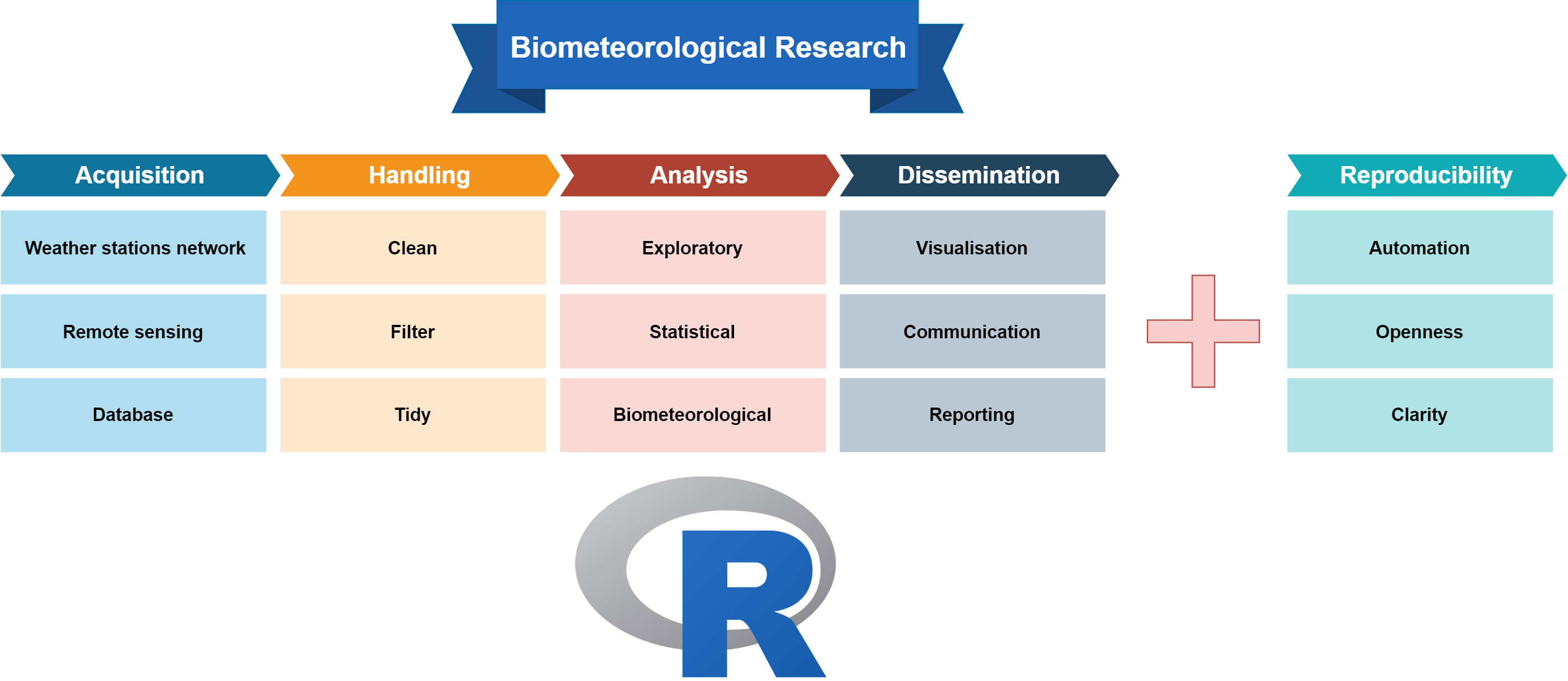
Nowadays, an important concern in science is reproducibility. As Powers and Hampton indicate [54] “Reproducibility is a key tenet of the scientific process that dictates the reliability and generality of results and methods”. It is exceedingly difficult—almost impossible—to conduct reproducible science or research without automation and open procedures and methodologies. When the research workflow consists of clicks and many different software tools, the reproduction is impossible (Figure 2).
The most important reason for shifting from the classic research workflow to a code-enhanced workflow is to achieve automation and reproducibility. Working with a programming language, we can form an uninterrupted chain of processes, starting from the raw data and ending with the dissemination of the results. The programming language itself is the language to communicate with the computer. Most of them have their own strict grammar and syntax.
The automation due to a programming language offers, first of all, faster data processing. The analysis of scientific datasets sometimes consumes weeks of valuable research time. Each project (which may include field measurements, remote sensing processes, simulations or modelling) can yield a vast amount of data files. Each of these files must be handled repetitively in order to open it, examine the content and sometimes pre-process them in order to bring them into the correct format or structure. Probably, the modified content of the data files should be added to or merged with other data files. Doing the above process manually makes research a time and money sink.
Moreover, by doing manual data processes repeatedly, we increase the probability of making mistakes. The automation of the research via programming gives us the potential to avoid checking each and every result’s products, such as tables, graphs and output data files. The only thing we must check is our code (the script). The automation procedure can be shorter using “packages”. That is why some programming languages have incorporated functions libraries in the form of packages. By loading a package, the user obtains new ready-to-use functions, compiled codes, and sometimes sample data. Moreover, packages are accompanied by documentation and vignettes about the package’s usage. Hence, the researcher does not have to analytically write down code for all the processes but can load the appropriate packages and use the predefined functions. As shown in Figure 1, automation is a part of reproducibility, and Figure 2 illustrates that the necessary “ingredient” for achieving the gold standard of full replication is code (programming language script).
3. The R Biometeorological Research Workflow
Therefore, in order to avoid all these drawbacks of the classic research workflow, such as spending time on learning to use new software or the high probability of making mistakes, and at the same time to achieve clear, open and reproducible research, we need to work with a programming language. At this point, we have to remark that almost all programming languages can achieve every process, but the big question is what it costs. Some languages are extremely fast and efficiently utilise the processing power of the computer. Other languages are very capable of creating a mobile phone or other user-friendly applications, but in the academic and research community, the fundamental questions are how much time the researcher needs to become familiar with each tool and if this time investment is scientifically profitable. Hence, in research, we need a highly readable programming language, with a clear and simple syntax which does not require professional skills and degrees in computer science to use it. To be clear, the research community needs a programming language for non-programmers. R has all the beneficial attributes to be the primary tool for biometeorological research because it is a general-purpose data analysis language which can be easily and quickly learned without any previous coding experience.
3.1. R’s main Characteristics
Briefly, we can describe R as a modern, functional programming language that allows for the rapid development of ideas, together with object-oriented features for rigorous software development [55]. Moreover, it is particularly important that R is a multiplatform, free, and open-source software. That allows every research group to use it without limitations, independent of the funding resources or the operating systems the researchers use, and the open-source characteristic is a guarantee for the quick development of new tools. R mainly consists of the language plus the run-time graphic environment and the system debugger. There are many implementations of integrated development environments (IDEs), such as RStudio®, Jupyter® with R kernel or R Tools for Visual Studio®, for easy and unobstructed software or code script development. The language was introduced by Ihaka and Gentleman [56] in 1996 as a combination of two previous computer languages, S and Scheme [57]. The R community is highly active and talented; hence, there is a vast number of free tutorials, forums, training datasets and documentations.
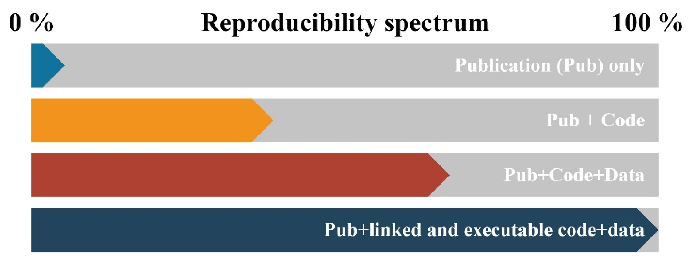
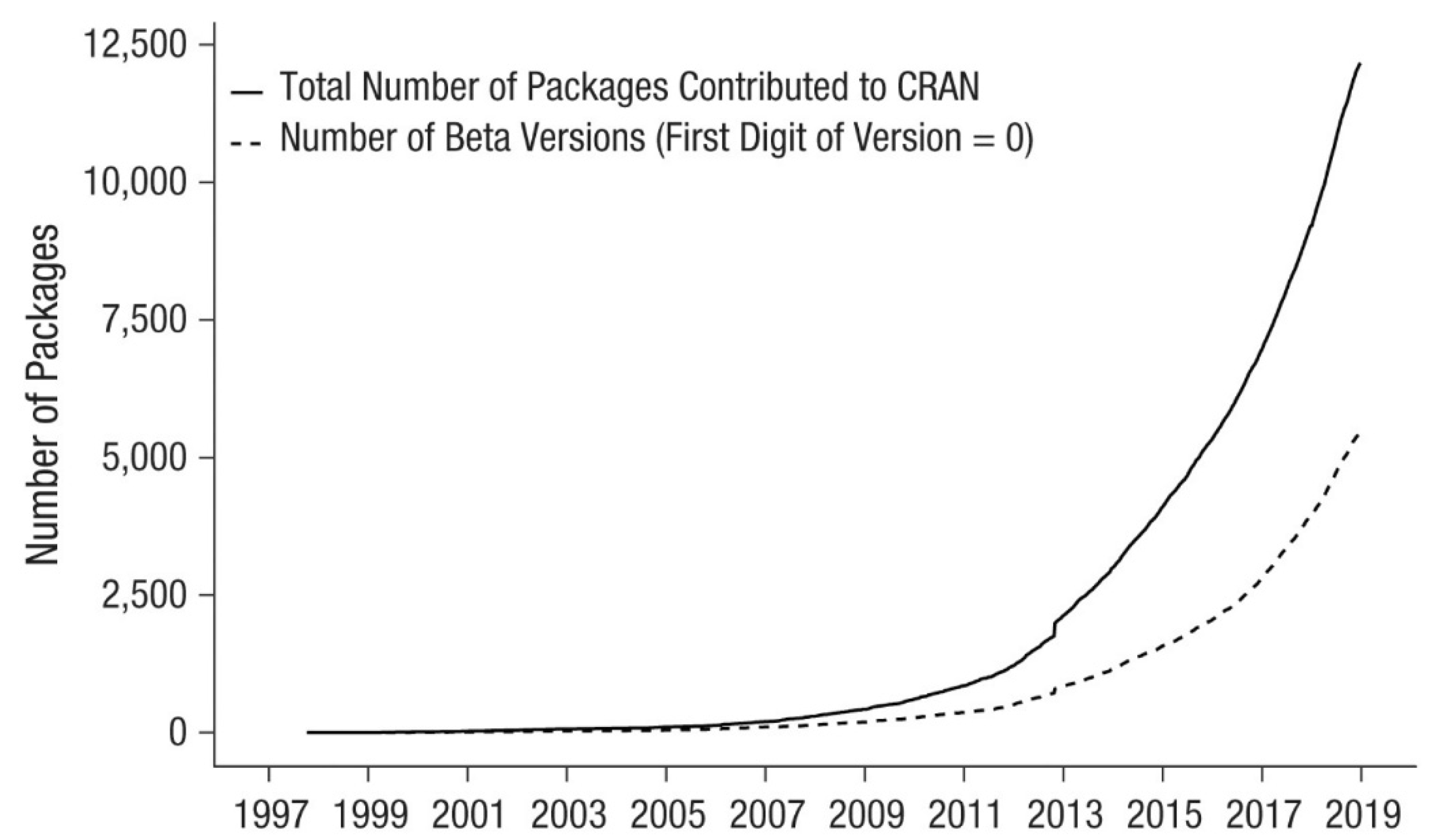
Additionally, the R community develops the packages (the specialised libraries) at an almost exponential productivity rate (Figure 3). Most of them are available from the Comprehensive R Archive Network (CRAN) online repository of sites which carry identical material, consisting of R distribution(s), contributed extensions, documentation for R, and binaries. The number of packages is far higher than 12,500 (in 2019) because there are more repositories, such as Bioconductor and GitHub containing hundreds of R packages. It is very important that the R user is not obliged to create “environments” or to check for versioning compatibility between the core of the language and the packages, or to take care of loading dependent packages separately. This is a priceless characteristic for scientists without a programming background.
At this point, we must mention the disadvantages of R. First, R uses only the physical memory (RAM) of the computer. This is an apparent restriction to our programming ambitions but the new generations of personal computers (PCs) come by default with an adequate amount of RAM to handle even Big Data. Besides, there are many techniques and specialised packages for data management. Another drawback of R is its speed since it is not made for multiprocessor processing by default. Nevertheless, there are R packages that enable parallel computing with R. The last disadvantage of the R language is that it cannot produce executable files. That means that we cannot send an application to our colleagues, but we can send the code and run this on their computer. This weakness of R is probably a hidden strength because it invigorates the research transparency and openness.
In the following sections, there is a selection of packages covering the needs of the common biometeorological research accompanied by tables with the names of the packages and short descriptions (The name of each package in the tables is an active link to the source of the package).
3.2. Data Acquisition with R
The foremost action of the research group is to acquire the data for the analysis. In atmospheric sciences such as biometeorology, there is a big variety of data sources. This means, as already mentioned, that a biometeorologist may collect field data from various types of loggers or scanned questionnaires. Moreover, for the same project, the research group could be obliged to use data from the registry of a hospital, from the meteorological service and so on. The result of the above is a variety of formats in terms of files with a different extension and in terms of files with the same extension but a different structure. We can separate the data acquisition in data input/output from local sources and web database sources (Table 1).
With the term local, we mean the data distribution via any means (e.g., USB stick, email, cloud services), and with the term web sources, we mean the distribution via a structured web service which provides an API (application programming interface) as a contact point. From the plethora of R’s data input packages, we suggest “readr” [58] as a solution for a fast and friendly way to read rectangular data in csv, tsv and fwf format. As Peng [59] pinpoint, “readr functions such as read_csv (reading csv files) optimize dramatically the reading speed of R”.
Another very useful package for reading and writing the widely used spreadsheets files is “xlsx” [60]. It is an easy-to-use package that gives us the ability to read the content of an xlsx file and its separate worksheets. It is very popular among R users because it enables the uninterrupted data flow from the non-R-literate scientific community to the R users and vice versa. For the same purpose, we can utilise the “foreign” [61] and “haven” [62] packages because they are made for easy input and output data for SPSS, SAS, Minitab and Stata native formats. These packages can read and import data created by the above widely used statistic software and export datasets to a readable format enhancing interoperability. Moreover, the “feather” package [63] is made to read and write feather files, a lightweight binary columnar data store designed for maximum speed. With this package we can afford the weight of big data files securely.
Apart from the aforementioned packages, base R can easily and accurately import every type of data file if the user describes the structure and the characteristics of its contents. The packages, first of all, are a shortcut if we want to bypass all the detailed coding, achieving higher processing speed.
As was already mentioned, in biometeorology, researchers use data from big databases; they offer their content via web services and APIs, like NASA, COPERNICUS and others. The R community has already created the related data for an easy and uninterrupted connection with the databases. In Table 1, users can find a selection of the most popular packages for data retrieval in the atmospheric content web databases. The “rnoaa” package [64] is dedicated to the NOAA (National Oceanic and Atmospheric Administration) data sources from current weather data to sea ice and historic recordings. With almost a single line of R code, the researcher can define the type of data, the location (if needed), the time period and other details and download them. The “nasapower” package [65] is specialised in NASA-POWER dataset acquisition with enhanced functionality. A very useful package is “Copernicus” [66] that is specialised in Global Land Vegetation Products and their products, such as NDVI, LAI and other indices. Moreover, an example of a widely used dataset for a wide range of research are the MODIS satellite products. The “MODIS” package [67] provides automated access to global online data archives.
Another valuable package for biometeorological research is the “rWBclimate” [68] that can give access to the World Bank’s climate circulation models data. A vast amount of useful data derived from EUMETSAT is available with the usage of the “cmsaf” package [69] in the widely used format of NetCDF. Finally, the “NASAaccess” package [70] with more than 50 integrated functions give access to gridded Ascii files containing climate and weather information. Of course, there are a few dozens of packages made for acquiring data from web bases such as Landsat, ESA and so on. All the above data can also become accessible using a web browser or an FTP client software but using R packages makes the process automatic, quick, and accurate in quite an easy way with two to three lines of code.
3.3. Data Handling with R
As a data analysis-oriented language, R is highly effective in handling and managing data in an unprecedented way. Researchers are literally “educated” on how to handle and what can do with their data by the software they used. The limitations of the software are the limitations of the research practice and, at the end of the day, are the limitations of the scientist’s ideas. The R language preserves absolute freedom on data handling and manipulation. If there is a central argument on choosing the coding practice instead of using data analysis or statistical software, this is the freedom and subsequent capability of managing the data powerfully.
The most popular R packages for data handling are “data.table” [71] and “dplyr” [72]. The first is one level above base R and provides all the necessary functions (tools) to subset, rename, summarise, merge or group, bind and, of course, do every calculation we need between columns or rows of a data table or between separate data tables. On the other hand, “dplyr” has introduced six “verbs” (i.e., functions) in order to do all the work “data.table” functions do, but in a different syntax. The last version (1.0) of “dplyr” improved its speed, and with its neat syntax, it is the flagship of data handling in the R world. As presented in Table 2, the next widely used data handling package is “reshape2” [73]. The main purpose of this package is the reshaping of the data format from the long to the wide structure and vice versa. As Wickham [74] mentioned, this process is usually tedious and frustrating. The “reshape2”, gives us two functions to do all this important work. Some of the basic modifications of data table structures can be made with the “pivot_longer” and “pivot_wider” functions of the “dplyr” package. The package “lubridate” [75] is focused on the date and time parts of our datasets. It contains some particularly useful functions for handling and parsing such data. In addition, it gives new capabilities on time zones or time-series data.
The introduced packages are a subset of a big number of R packages for data handling (e.g., stringr, tidyr). However, those four packages are enough for easy, fast and accurate data handling processes. It is worth mentioning that during coding synthesis we can use every package we need, and all of them are made to collaborate with the others.
3.4. Biometeorological Data Analysis with R
As anticipated, the R community has already created specialised packages for biometeorological research. The “comf” package [76] is made to easily calculate some of the most widely used human thermal comfort indices such as PMV (Predicted Mean Vote) and PPD (Predicted Percentage Dissatisfied) [77] or estimate synthetic parameters such as MRT (Mean Radiant Temperature). In total, in this package, more than 20 indices and related biometeorological (or bioclimatological) parameters are incorporated. The following related package is “ClimInd” [78] which gives us the functions to calculate more than 100 climatic and bioclimatic indices (Table 3). The variety of the indices is great, covering a spectrum from temperature-based to tourism indices.
Another very promising R package for human biometeorological index calculations is “rBiometeo” [79]. The predefined functions of this package vary from human energy balance indices such as PMV to the classic thermohygrometric index (THI). In order to feed the biometeorological indices with input data we can use the “climate” R package [80] that is specialised in the automation of meteorological data downloading. It is well connected with OGIMET, NOAA and other publicly available databases. Moreover the “RNCEP” package [81] contains functions to temporally aggregate data, producing user-defined variables, and to visualise these data on a map, encouraging the exploration of relationships between biological systems and atmospheric conditions.
In biometeorological research, the conversion between metric systems and units is a common practice. The “weathermetrics” package [82] provides ready-to-use functions to facilitate all the possible unit and metrics conversions. The catalogue of the biometeorologically related R packages is exceedingly long because, in research practice, we use functions from packages oriented or made for other scientific disciplines. Along with the functions of the above packages, we can use advanced mathematics functions such as Generalized Additive Models from the “mgcv” package [83] or propensity score analysis with the “MatchIt” package [84]. Moreover, advanced R users can create and publish their biometeorological R package, or they can define and apply their own functions.
3.5. Results Dissemination with R
Probably one of R’s most powerful attributes is the communication of the research results to the broad public. It is well known that with R, we can easily create beautiful and neat graphs, and we can report the research results in the form of a web page (HTML), slides or any type and format of documents.
A very quick and effective R package for plotting is the “lattice” [85]. It can plot univariate and multivariate data graphs with almost a line of code. It is very famous for the trellis graphs which display the distribution of a variable or the relationship between variables, separately for each level or more other variables [86]. On the other hand, the “ggplot2” package [87] is the flagship of the R graphics. The “gg” means grammar of graphics and Hadley Wickham [88], the author of this package, introduced a new way of working with data plots. The main concept is that the graph consists of five separate layers: the “mapping”, which contains the set of aesthetics, the “data” which contains the presented dataset, the “geom” which describes the type of the data illustration (e.g., line, dot, boxplot), the “stat” which describes the statistical transformation we probably want to do with data, and the “position” which adjusts the overlapping method of the objects. The above layers are not mandatory for every graph we create. The justification for using ggplot2 for data graphs is a long catalogue of clear advantages, such as automatic and easy legends and colours (with pallets), lots of default characteristics, easy faceting, flexibility on changing systems from cartesian to logarithmic and so on. Finally, the usage of the ggplot2 package gives us the privilege of unrestricted choices about the graphs’ output format, resolution and size. All in all, it is an absolutely professional tool for scientific graphs. The next R package (Table 4) for results dissemination is “plotly” [89], which was initially created for the Python programming language. This unique tool creates interactive, publication-quality graphs. In addition, its ability to present 3D plots in a very effective way, along with the production of animated plots, ranks “plotly” among the essential tools for results dissemination.
Since the communication of research results is not only a matter of graphs, scientists need tools for reporting and sharing their findings. There is a group of R packages which can embody the R functional code inside a classic digital document, or an HTML page via automatic compilation. Hence, the “rmarkdown” package [90] helps us to create dynamic analysis documents that combine code with rendered output. With this package, the biometeorological results can be combined with the data and the related code into a polished document which can be the state of the art in terms of reproducibility. The package “rmarkdown” gives outputs in doc, pdf and HTML using the markdown [91] and free text syntax, enriched with code chunks.
Nowadays, it is common for research groups to communicate their findings in blogs. Hence, the “blogdown” R package [92] is an ideal solution because it is dedicated to creating web pages made with “rmarkdown”. This package in collaboration with a static site generator can create web sites (blogs) in several minutes. In addition to the above, the “bookdown” R package [93] facilitates writing books and long-form articles and reports with the rmarkdown syntax. With this excellent package, authors can easily create printer-ready books and e-books with automations in terms of their style and structure. Of course, there is a group of predefined functions that create a table of contents, indices and other parts of a book.
The last R package which is very useful for the communication and dissemination of biometeorological research results is “shiny” [94]. With this tool, scientists can create interactive web applications with R code. In this way, the scientific community can share the results, or the data by an integrated graphic environment that makes them explorable by the public. The shiny web applications can contain maps and interactive graphs (e.g., bar plots, box plots and pie charts). Apart from the visual parts of the web applications, parts of text and code can coexist. Finally, the user of shiny-made applications can produce outputs in doc and pdf formats or can download the created images or the data results in csv and other formats.
3.6. A Reproducible Research Example with the R Language
In order to clarify the way in which R empowers the reproducibility and the automation of biometeorological research, a full example is added as Supplementary Material. This example is presented as an Rmarkdown (.Rmd) file, which is a hydridic file containing the descriptive text and the R code. When the researcher runs this file, a new text rendered file (pdf) is produced along with the codes output (graphs and a data table). All the above is also available from the GitHub repository at https://github.com/icharalamp/Atmosphere_mdpi_R_as_a_tool.
4. Conclusions
As analysed above, the R language covers the entire spectrum of biometeorological research needs. This subset of the presented packages proves that the researcher can cover all the essential yet specific needs from data acquisition to results dissemination. We pinpointed that R’s base language syntax and its packages are by default fully documented. The wide and productive R community provides invaluable and continuous help from an amateur to a professional level. Moreover, the power of this language is not only the more than 15,000 packages but the ability of the user to easily create their own package and share it with the community through the official repositories (e.g., CRAN, GitHub and Bioconductor). The obligated “openness” of R’s code is a way for deeper and clean collaboration. Last but not least, the language’s ability to import and export data in any known format allows R users to be in intimate connection with the non-R-literate scientific community. Finally, as is obvious, the R language could be the lingua franca in biometeorological research.
Supplementary Materials
The following are available online at https://www.mdpi.com/2073-4433/11/7/682/s1, File1: RMarkdown file containing text and code. File2: PDF file rendered from the RMarkdown file.
Funding
This research received no external funding.
Conflicts of Interest
The author declares no conflict of interest.
References
- Tromp, S.W. Human biometeorology. Int. J. Biometeorol. 1963, 7, 145–158. [Google Scholar] [CrossRef]
- Tout, D.G. Biometeorology. Prog. Phys. Geogr. Earth Environ. 1987, 11, 473–486. [Google Scholar] [CrossRef]
- Flemming, G. The importance of air quality in human biometeorology. Int. J. Biometeorol. 1996, 39, 192–196. [Google Scholar] [CrossRef] [PubMed]
- McGregor, G.R. Human biometeorology. Prog. Phys. Geogr. Earth Environ. 2012, 36, 93–109. [Google Scholar] [CrossRef]
- Höppe, P. The physiological equivalent temperature—A universal index for the biometeorological assessment of the thermal environment. Int. J. Biometeorol. 1999, 43, 71–75. [Google Scholar] [CrossRef]
- Algeciras, J.A.; Consuegra, L.G.; Matzarakis, A. Spatial-temporal study on the effects of urban street configurations on human thermal comfort in the world heritage city of Camagüey-Cuba. Build. Environ. 2016, 101, 85–101. [Google Scholar] [CrossRef]
- Charalampopoulos, I.; Nouri, A.S. Investigating the behaviour of human thermal indices under divergent atmospheric conditions: A sensitivity analysis approach. Atmosphere 2019, 10, 580. [Google Scholar] [CrossRef] [Green Version]
- de Abreu-Harbich, L.V.; Labaki, L.C.; Matzarakis, A. Effect of tree planting design and tree species on human thermal comfort in the tropics. Landsc. Urban Plan. 2015, 138, 99–109. [Google Scholar] [CrossRef]
- Giannaros, T.M.; Kotroni, V.; Lagouvardos, K.; Matzarakis, A. Climatology and trends of the Euro-Mediterranean thermal bioclimate. Int. J. Climatol. 2018, 38, 3290–3308. [Google Scholar] [CrossRef]
- Kántor, N.; Chen, L.; Gál, C.V. Human-biometeorological significance of shading in urban public spaces—Summertime measurements in Pécs, Hungary. Landsc. Urban Plan. 2018, 170, 241–255. [Google Scholar] [CrossRef]
- Kaplan, S.; Peterson, C. Health and environment: A psychological analysis. Landsc. Urban Plan. 1993, 26, 17–23. [Google Scholar] [CrossRef] [Green Version]
- Lin, T.-P.; Matzarakis, A. Tourism climate and thermal comfort in Sun Moon Lake, Taiwan. Int. J. Biometeorol. 2008, 52, 281–290. [Google Scholar] [CrossRef] [PubMed]
- Matzarakis, A.; Mayer, H. The extreme heat wave in Athens in July 1987 from the point of view of human biometeorology. Atmos. Environ. Part B Urban Atmos. 1991, 25, 203–211. [Google Scholar] [CrossRef]
- Nastos, P.T.; Matzarakis, A. The effect of air temperature and human thermal indices on mortality in Athens, Greece. Theor. Appl. Climatol. 2012, 108, 591–599. [Google Scholar] [CrossRef]
- Bruse, M.; Fleer, H. Simulating surface–plant–air interactions inside urban environments with a three dimensional numerical model. Environ. Model. Softw. 1998, 13, 373–384. [Google Scholar] [CrossRef]
- Fröhlich, D.; Matzarakis, A. spatial estimation of thermal indices in Urban Areas—Basics of the SkyHelios Model. Atmosphere 2018, 9, 209. [Google Scholar] [CrossRef] [Green Version]
- Lindberg, F.; Grimmond, C.S.B.; Gabey, A.; Huang, B.; Kent, C.W.; Sun, T.; Theeuwes, N.E.; Järvi, L.; Ward, H.C.; Capel-Timms, I.; et al. Urban multi-scale environmental predictor (UMEP): An integrated tool for city-based climate services. Environ. Model. Softw. 2018, 99, 70–87. [Google Scholar] [CrossRef]
- Matzarakis, A.; Rutz, F.; Mayer, H. Modelling radiation fluxes in simple and complex environments—application of the RayMan model. Int. J. Biometeorol. 2007, 51, 323–334. [Google Scholar] [CrossRef]
- Gaughan, J.; Lacetera, N.; Valtorta, S.E.; Khalifa, H.H.; Hahn, L.; Mader, T. Response of domestic animals to climate challenges. In Biometeorology for Adaptation to Climate Variability and Change; Ebi, K.L., Burton, I., McGregor, G.R., Eds.; Springer: Dordrecht, The Netherlands, 2009; pp. 131–170. ISBN 978-1-4020-8921-3. [Google Scholar]
- Hatfield, J.L.; Dold, C. Agroclimatology and wheat production: Coping with climate change. Front. Plant Sci. 2018, 9. [Google Scholar] [CrossRef] [Green Version]
- Hondula, D.M.; Balling, R.C.; Andrade, R.; Scott Krayenhoff, E.; Middel, A.; Urban, A.; Georgescu, M.; Sailor, D.J. Biometeorology for cities. Int. J. Biometeorol. 2017, 61, 59–69. [Google Scholar] [CrossRef]
- Sofiev, M.; Bousquet, J.; Linkosalo, T.; Ranta, H.; Rantio-Lehtimaki, A.; Siljamo, P.; Valovirta, E.; Damialis, A. Pollen, Allergies and Adaptation. In Biometeorology for Adaptation to Climate Variability and Change; Ebi, K.L., Burton, I., McGregor, G.R., Eds.; Springer: Dordrecht, The Netherlands, 2009; pp. 75–106. ISBN 978-1-4020-8921-3. [Google Scholar]
- Vasconcelos, J.; Freire, E.; Almendra, R.; Silva, G.L.; Santana, P. The impact of winter cold weather on acute myocardial infarctions in Portugal. Environ. Pollut. 2013, 183, 14–18. [Google Scholar] [CrossRef] [PubMed]
- Quinn, A.; Tamerius, J.D.; Perzanowski, M.; Jacobson, J.S.; Goldstein, I.; Acosta, L.; Shaman, J. Predicting indoor heat exposure risk during extreme heat events. Sci. Total Environ. 2014, 490, 686–693. [Google Scholar] [CrossRef] [PubMed] [Green Version]
- Telfer, S.; Obradovich, N. Local weather is associated with rates of online searches for musculoskeletal pain symptoms. PLoS ONE 2017, 12, e0181266. [Google Scholar] [CrossRef] [PubMed] [Green Version]
- Charalampopoulos, I.; Nastos, P.T.; Didaskalou, E. Human thermal conditions and North Europeans’ web searching behavior (Google Trends) on mediterranean touristic destinations. Urban Sci. 2017, 1, 8. [Google Scholar] [CrossRef] [Green Version]
- Samson, D.R.; Crittenden, A.N.; Mabulla, I.A.; Mabulla, A.Z.P. The evolution of human sleep: Technological and cultural innovation associated with sleep-wake regulation among Hadza hunter-gatherers. J. Hum. Evol. 2017, 113, 91–102. [Google Scholar] [CrossRef]
- Charalampopoulos, I. A comparative sensitivity analysis of human thermal comfort indices with generalized additive models. Theor. Appl. Climatol. 2019. [Google Scholar] [CrossRef]
- Nouri, A.S.; Charalampopoulos, I.; Matzarakis, A. Beyond singular climatic variables—Identifying the dynamics of wholesome Thermo-Physiological factors for existing/future human thermal comfort during hot dry mediterranean summers. Int. J. Environ. Res. Public Health 2018, 15, 2362. [Google Scholar] [CrossRef] [Green Version]
- Chinazzo, G.; Wienold, J.; Andersen, M. Daylight affects human thermal perception. Sci. Rep. 2019, 9. [Google Scholar] [CrossRef] [PubMed]
- Półrolniczak, M.; Tomczyk, A.M.; Kolendowicz, L. Thermal conditions in the city of Poznań (Poland) during selected heat waves. Atmosphere 2018, 9, 11. [Google Scholar] [CrossRef] [Green Version]
- Schweiker, M.; Wagner, A. Influences on the predictive performance of thermal sensation indices. Build. Res. Inf. 2017, 45, 745–758. [Google Scholar] [CrossRef]
- Quinn, A.; Kinney, P.; Shaman, J. Predictors of summertime heat index levels in New York City apartments. Indoor Air 2017, 27, 840–851. [Google Scholar] [CrossRef] [PubMed]
- Kolendowicz, L.; Półrolniczak, M.; Szyga-Pluta, K.; Bednorz, E. Human-biometeorological conditions in the southern Baltic coast based on the universal thermal climate index (UTCI). Theor. Appl. Climatol. 2018, 134, 363–379. [Google Scholar] [CrossRef] [Green Version]
- Just, M.G.; Nichols, L.M.; Dunn, R.R. Human indoor climate preferences approximate specific geographies. R. Soc. Open Sci. 2019, 6, 180695. [Google Scholar] [CrossRef] [PubMed] [Green Version]
- Salamone, F.; Bellazzi, A.; Belussi, L.; Damato, G.; Danza, L.; Dell’Aquila, F.; Ghellere, M.; Megale, V.; Meroni, I.; Vitaletti, W. Evaluation of the visual stimuli on personal thermal comfort perception in real and virtual environments using machine learning approaches. Sensors 2020, 20, 1627. [Google Scholar] [CrossRef] [PubMed] [Green Version]
- Silva, A.S.; Almeida, L.S.S.; Ghisi, E. Decision-making process for improving thermal and energy performance of residential buildings: A case study of constructive systems in Brazil. Energy Build. 2016, 128, 270–286. [Google Scholar] [CrossRef]
- Charalampopoulos, I.; Tsiros, I.; Chronopoulou-Sereli, A.; Matzarakis, A. A note on the evolution of the daily pattern of thermal comfort-related micrometeorological parameters in small urban sites in Athens. Int. J. Biometeorol. 2014, 59, 1223–1236. [Google Scholar] [CrossRef] [PubMed]
- Steiner, J.L.; Hatfield, J.L. Winds of change: A century of agroclimate research. Agron. J. 2008, 100, S-132–S-152. [Google Scholar] [CrossRef] [Green Version]
- Lees, J.M. Open and free: Software and scientific reproducibility. Seismol. Res. Lett. 2012, 83, 751–752. [Google Scholar] [CrossRef]
- Peng, R.D. Reproducible research in computational science. Science 2011, 334, 1226–1227. [Google Scholar] [CrossRef] [Green Version]
- Stodden, V. Reproducible research: Tools and strategies for scientific computing. Comput. Sci. Eng. 2012, 14, 11–12. [Google Scholar] [CrossRef] [Green Version]
- Lowndes, J.S.S.; Best, B.D.; Scarborough, C.; Afflerbach, J.C.; Frazier, M.R.; O’Hara, C.C.; Jiang, N.; Halpern, B.S. Our path to better science in less time using open data science tools. Nat. Ecol. Evol. 2017, 1, 0160. [Google Scholar] [CrossRef] [PubMed] [Green Version]
- Peng, R.D.; Matsui, E. The Art of Data Science; Leanpub: Victoria, BC, Canada, 2015; ISBN 978-1-365-06146-2. [Google Scholar]
- van den Burg, G.J.J.; Nazábal, A.; Sutton, C. Wrangling messy CSV files by detecting row and type patterns. Data Min. Knowl. Disc. 2019, 33, 1799–1820. [Google Scholar] [CrossRef] [Green Version]
- Wickham, H. Tidy Data. J. Stat. Softw. 2014, 59, 1–23. [Google Scholar] [CrossRef] [Green Version]
- Han, J.; Kamber, M.; Pei, J. Data Mining Concepts and Techniques; Elsevier: Amsterdam, The Netherlands, 2011; ISBN 978-0-12-381479-1. [Google Scholar]
- Márquez, F.P.G.; Lev, B. Big Data Management; Springer International Publishing: Berlin/Heidelberg, Germany, 2016; ISBN 978-3-319-45498-6. [Google Scholar]
- Leek, J. The Elements of Data Analytic Style; Leanpub: Victoria, BC, Canada, 2015. [Google Scholar]
- Sandve, G.K.; Nekrutenko, A.; Taylor, J.; Hovig, E. Ten simple rules for reproducible computational research. PLoS Comput. Biol. 2013, 9, e1003285. [Google Scholar] [CrossRef] [Green Version]
- Hothorn, T.; Everitt, B.S. A Handbook of Statistical Analyses Using R; CRC press: Boca Raton, FL, USA, 2014; ISBN 1-4822-0458-4. [Google Scholar]
- Weiss, N.A.; Weiss, C.A. Introductory Statistics; Pearson; Addison-Wesley: Boston, MA, USA, 2008; ISBN 0-321-39361-9. [Google Scholar]
- Munafò, M.R.; Nosek, B.A.; Bishop, D.V.M.; Button, K.S.; Chambers, C.D.; du Sert, N.P.; Simonsohn, U.; Wagenmakers, E.-J.; Ware, J.J.; Ioannidis, J.P.A. A manifesto for reproducible science. Nat. Hum. Behav. 2017, 1, 1–9. [Google Scholar] [CrossRef] [Green Version]
- Powers, S.M.; Hampton, S.E. Open science, reproducibility, and transparency in ecology. Ecol. Appl. 2019, 29, e01822. [Google Scholar] [CrossRef] [Green Version]
- Eglen, S.J. A quick guide to teaching R Programming to computational biology students. PLoS Comput. Biol. 2009, 5, e1000482. [Google Scholar] [CrossRef] [Green Version]
- Ihaka, R.; Gentleman, R.R. A language for data analysis and graphics. J. Comput. Graph. Stat. 1996, 5, 299–314. [Google Scholar] [CrossRef]
- Grunsky, E.C.R. A data analysis and statistical programming environment—An emerging tool for the geosciences. Comput. Geosci. 2002, 28, 1219–1222. [Google Scholar] [CrossRef]
- Wickham, H.; Hester, J.; Francois, R. Readr: Read Rectangular Text Data. Available online: https://CRAN.R-project.org/package=readr (accessed on 25 April 2020).
- Peng, R.D. R Programming for Data Science; Leanpub: Victoria, BC, Canada, 2016; ISBN 978-1-365-05682-6. [Google Scholar]
- Dragulescu, A.; Arendt, C. Xlsx: Read, Write, Format Excel 2007 and Excel 97/2000/XP/2003 Files. Available online: https://CRAN.R-project.org/package=xlsx (accessed on 10 May 2020).
- R Core Team foreign. Read Data Stored by “Minitab”, “S”, “SAS”, “SPSS”, “Stata”, “Systat”, “Weka”, “dBase”. Available online: https://CRAN.R-project.org/package=foreign (accessed on 12 May 2020).
- Wickham, H.; Miller, E. Haven: Import and Export “SPSS”, “Stata” and “SAS” Files. Available online: https://CRAN.R-project.org/package=haven (accessed on 25 April 2020).
- Wickham, H. feather: R Bindings to the Feather “API”. Available online: https://CRAN.R-project.org/package=feather (accessed on 25 April 2020).
- Chamberlain, S. Rnoaa: “NOAA” Weather Data from R. Available online: https://CRAN.R-project.org/package=rnoaa (accessed on 10 May 2020).
- Sparks, A.H. Nasapower: NASA POWER API Client. Available online: https://CRAN.R-project.org/package=nasapower (accessed on 12 May 2020).
- Stevens, A. Copernicus. Available online: https://github.com/antoinestevens/copernicus (accessed on 4 June 2020).
- Mattiuzzi, M.; Detsch, F. MODIS: Acquisition and Processing of MODIS Products. Available online: https://CRAN.R-project.org/package=MODIS (accessed on 12 May 2020).
- Hart, E. RWBclimate: A package for accessing World Bank climate data. Available online: https://CRAN.R-project.org/package=rWBclimate (accessed on 12 May 2020).
- Kothe, S. Cmsaf: Tools for CM SAF NetCDF Data. Available online: https://CRAN.R-project.org/package=cmsaf (accessed on 12 May 2020).
- Mohammed, I. NASAaccess: Downloading and reformatting tool for NASA Earth observation data products. Available online https://github.com/nasa/NASAaccess: (accessed on 12 May 2020).
- Dowle, M.; Srinivasan, A. Data.table: Extension of ‘data.frame’. Available online: https://CRAN.R-project.org/package=data.table (accessed on 10 May 2020).
- Wickham, H.; François, R.; Henry, L.; Müller, K. Dplyr: A Grammar of Data Manipulation. Available online: https://CRAN.R-project.org/package=dplyr (accessed on 25 April 2020).
- Wickham, H. Reshape2: Flexibly Reshape Data: A Reboot of the Reshape Package. Available online: https://CRAN.R-project.org/package=reshape2 (accessed on 25 April 2020).
- Wickham, H. Reshaping data with the reshape package. J. Stat. Softw. 2007, 21, 1–20. [Google Scholar] [CrossRef]
- Spinu, V.; Grolemund, G.; Wickham, H. Lubridate: Make Dealing with Dates a Little Easier. Available online: https://CRAN.R-project.org/package=lubridate (accessed on 12 May 2020).
- Schweiker, M.; Mueller, S.; Kleber, M.; Kingma, B.; Shukuya, M. Comf: Functions for Thermal Comfort Research. Available online: https://CRAN.R-project.org/package=comf (accessed on 15 May 2020).
- Fanger, P.O. Thermal Comfort. Analysis and Applications in Environmental Engineering; McGraw-Hill Book Company: New York, NY, USA, 1970; ISBN 978-0-07-019915-6. [Google Scholar]
- Reig-Gracia, F.; Vicente-Serrano, S.M.; Dominguez-Castro, F.; Bedia-Jiménez, J. ClimInd: Climate Indices. Available online: https://CRAN.R-project.org/package=ClimInd (accessed on 10 May 2020).
- Crisci, A.; Morabito, M. RBiometeo: Biometeorological Functions in R. Available online: https://github.com/alfcrisci/rBiometeo (accessed on 15 May 2020).
- Czernecki, B.; Glogowski, A.; Nowosad, J. Climate: Interface to Download Meteorological (and Hydrological) Datasets. Available online: https://CRAN.R-project.org/package=climate (accessed on 17 May 2020).
- Kemp, M.U.; van Loon, E.E.; Shamoun-Baranes, J.; Bouten, W. RNCEP: Global weather and climate data at your fingertips. Methods Ecol. Evol. 2012, 3, 65–70. [Google Scholar] [CrossRef]
- Anderson, B.; Peng, R.; Ferreri, J. Weathermetrics: Functions to Convert Between Weather Metrics. Available online: https://CRAN.R-project.org/package=weathermetrics (accessed on 15 May 2020).
- Wood, S. Mgcv: Mixed GAM Computation Vehicle with Automatic Smoothness Estimation. Available online: https://CRAN.R-project.org/package=mgcv (accessed on 19 May 2020).
- Ho, D.; Imai, K.; King, G.; Stuart, E. MatchIt: Nonparametric Preprocessing for Parametric Causal Inference. Available online: https://CRAN.R-project.org/package=MatchIt (accessed on 17 May 2020).
- Sarkar, D. Lattice: Trellis Graphics for R. Available online: https://CRAN.R-project.org/package=lattice (accessed on 5 February 2020).
- Kabacoff, R. R in Action. Data Analysis and Graphics with R; Manning: New York, NY, USA, 2011. [Google Scholar]
- Wickham, H.; Chang, W.; Henry, L.; Pedersen, T.L.; Takahashi, K.; Wilke, C.; Woo, K.; Yutani, H.; Dunnington, D. Ggplot2: Create Elegant Data Visualisations Using the Grammar of Graphics. Available online: https://CRAN.R-project.org/package=ggplot2 (accessed on 5 February 2020).
- Wickham, H. ggplot2: Elegant Graphics for Data Analysis; Springer: New York, NY, USA, 2016; ISBN 978-3-319-24277-4. [Google Scholar]
- Sievert, C.; Parmer, C.; Hocking, T.; Chamberlain, S.; Ram, K.; Corvellec, M.; Despouy, P. Plotly: Create Interactive Web Graphics via “plotly.js”. Available online: https://CRAN.R-project.org/package=plotly (accessed on 5 February 2020).
- Xie, Y.; Allaire, J.J.; Grolemund, G. R Markdown: The Definitive Guide; Chapman and Hall/CRC: New York, NY, USA, 2018; ISBN 978-1-138-35933-8. [Google Scholar]
- Gruber, J. Markdown. Available online: http://daringfireball.net/projects/markdown/ (accessed on 5 February 2020).
- Xie, Y. Blogdown: Create Blogs and Websites with R Markdown. Available online: https://CRAN.R-project.org/package=blogdown (accessed on 5 February 2020).
- Xie, Y. Bookdown: Authoring Books and Technical Documents with R Markdown. Available online: https://CRAN.R-project.org/package=bookdown (accessed on 5 February 2020).
- Chang, W.; Cheng, J.; Allaire, J.J.; Xie, Y.; McPherson, J. Shiny: Web Application Framework for R. Available online: https://CRAN.R-project.org/package=shiny (accessed on 5 February 2020).
Figure 1.
The classic biometeorological research workflow.

Figure 2.
The reproducibility spectrum, modified by Peng 2011 [41].
Figure 2.
The reproducibility spectrum, modified by Peng 2011 [41].

Figure 3.
The number of R packages contributed to the Comprehensive R Archive Network (CRAN) [58].
Figure 3.
The number of R packages contributed to the Comprehensive R Archive Network (CRAN) [58].


Table 1.
R packages data acquisition.
| Package Name | Short Description | |
|---|---|---|
| Manual (local) input | readr | Fast and friendly way to read rectangular data (like csv, tsv, and fwf). |
| xlxs | Provides tools to read and write xlsx files and control the appearance of the spreadsheet files. | |
| foreign | Reading and writing data stored by some versions of ‘Epi Info’, ‘Minitab’, ‘S’, ‘SAS’, ‘SPSS’, ‘Stata’, ‘Systat’, ‘Weka’ and ‘dBase’ files. | |
| haven | Reading and writing data stored by of ‘SAS’, ‘SPSS’, ‘Stata’. | |
| feather | Read and write in an easy-to-use binary file format (feather) for storing data frames. | |
| Web database acquisition | rnoaa | Is an R wrapper to many NOAA APIs. Select and download each type of data |
| nasapower | Making quick and easy to automate downloading from NASA POWER global meteorology, surface solar energy and climatology data. | |
| MODIS | Downloading and processing functionalities for the Moderate Resolution Imaging Spectroradiometer (MODIS). | |
| Copernicus | Downloading data from the COPERNICUS data portal through the fast HTTP access. | |
| rWBclimate | Download model predictions from 15 different global circulation models in 20-year intervals from the World Bank. Access historical data and create maps at 2 different spatial scales. | |
| cmsaf | Provides satellite-based climate data records of essential climate variables of the energy budget and water cycle. The data records are generally distributed in NetCDF format. | |
| NASAaccess | Can generate gridded ASCII tables of climate (CIMP5) and weather data (GPM, TRMM, GLDAS) needed to drive various hydrological models (e.g., SWAT, VIC, RHESSys). |
Table 2.
Data handling R packages.
| Package Name | Short Description |
|---|---|
| data.table | Integrated and quick data handling. |
| dplyr | A powerful package with a noticeably clear syntax to transform, summarise and do calculation into and between tabular data frames. |
| reshape2 | Is dedicated to the transformation processes between wide and long data frame format. |
| lubridate | Providing functions to deal with date and time formats and time spans. |
Table 3.
Biometeorological data analysis packages.
| Package Name | Short Description |
|---|---|
| comf | Calculates various common and less common thermal comfort indices, convert physical variables and evaluate the performance of thermal comfort indices. |
| ClimInd | Computes 138 standard climate indices at monthly, seasonal and annual resolution. |
| rBiometeo | Human thermal comfort and many biometeorological indices used in Institute of Biometeorology in Florence. Biometeorological indices used in Institute of Biometeorology in Florence |
| climate | Automized downloading of meteorological and hydrological data from publicly available repositories. |
| RNCEP | Contains functions to retrieve, organise and visualise weather data from the NCEP/NCAR Reanalysis and NCEP/DOE Reanalysis II datasets. |
| weathermetrics | Conversions between primary weather metrics. |
Table 4.
R packages for results dissemination.
| Package Name | Short Description | |
|---|---|---|
| Visualisation | lattice | High-level data visualisation system, with an emphasis on multivariate data. |
| ggplot2 | A system for ‘declaratively’ creating graphics, based on “The Grammar of Graphics”. | |
| plotly | An all-in-one interactive graphics package (3D and animated). | |
| Communication | rmarkdown | Writing functional reports with embedded code and its results in .doc, .pdf, HTML format. |
| blogdown | Publishing web pages created with rmarkdown. | |
| bookdown | Facilitating writing ebooks, ready to print books, long articles and reports. | |
| shiny | Building interactive web applications focused on data sharing. |
© 2020 by the author. Licensee MDPI, Basel, Switzerland. This article is an open access article distributed under the terms and conditions of the Creative Commons Attribution (CC BY) license (http://creativecommons.org/licenses/by/4.0/).
Share and Cite
MDPI and ACS Style
Charalampopoulos, I. The R Language as a Tool for Biometeorological Research. Atmosphere 2020, 11, 682. https://doi.org/10.3390/atmos11070682
AMA Style
Charalampopoulos I. The R Language as a Tool for Biometeorological Research. Atmosphere. 2020; 11(7):682. https://doi.org/10.3390/atmos11070682
Chicago/Turabian StyleCharalampopoulos, Ioannis. 2020. "The R Language as a Tool for Biometeorological Research" Atmosphere 11, no. 7: 682. https://doi.org/10.3390/atmos11070682
Note that from the first issue of 2016, this journal uses article numbers instead of page numbers. See further details here.