WRF Sensitivity Analysis in Wind and Temperature Fields Simulation for the Northern Sahara and the Mediterranean Basin

Abstract

Different configurations for the Weather Research and Forecasting (WRF) model were evaluated to improve wind and temperature fields predictions in the Northern Sahara and the Mediterranean basin. Eight setups, associated with different combinations of the surface layer physical parameters, the land surface model, and the grid nudging parameters, were considered. Numerical simulations covered the entire month of November 2017. Model results were compared with surface data from meteorological stations. The introduction of the grid nudging parameters leads to a general improvement of the modeled 10 m wind speed and 2 m temperature. In particular, nudging of wind speed parameter inside the planetary boundary layer (PBL) provides the most remarkable differences. In contrast, the nudging of temperature and relative humidity parameters inside the PBL may be switched off to reduce computational time and data storage. Furthermore, it was shown that the prediction of the 10 m wind speed and 2 m temperature is quite sensitive to the choice of the surface layer scheme and the land surface model. This paper provides useful suggestions to improve the setup of the WRF model in the Northern Sahara and the Mediterranean basin. These results are also relevant for topics related with the emission of mineral dust and sea spray within the Mediterranean region.

1. Introduction

The proper assessment of wind and temperature near the Earth’s surface (over sea and ground) is very important for many applications, including human comfort, wind energy, wave modeling, coastal meteorology, cyclone forecasting, and aerosols studies. In particular, the latter topic is important for a wide range of fields, since aerosols are a key component of the atmosphere, playing a pivotal role from global to local scales in climatology [1], oceanic biogeochemical cycles [2], cloud microphysics [3], cyclone development [4], air quality [5], visibility [6], and human health [7], to cite just a few examples.

Aerosol particles are derived from both continental and oceanic sources, and they can be of either natural or anthropogenic origin. They are mainly emitted by fossil fuel and biomass combustion; by deserts and seas, mainly during windy conditions; and occasionally by volcano eruptions. Despite huge uncertainties [8], sea spray is the largest single source of aerosol mass injected into the atmosphere at the global level, followed by desert dust [9]. The aerosol transport is strongly dependent on the meteorological conditions, in particular wind speed and direction.

It is important to point out that the simulation of the emission and transport of aerosol particles depends crucially on the accuracy of the simulated meteorology and on the precision of the surface layer (SL) schemes over land and ocean. Desert dust particles are produced by wind erosion and soil resuspension; sea spray aerosol is produced by a complex interaction between wind and waves. From the modeling point of view, the aeolian erosion in semi-arid regions occurs when a threshold value of the surface friction velocity is reached; this value depends on the soil moisture and the type of surface layer scheme that is implemented in numerical models [10,11], while for sea spray, a critical value of about 4 m s⁻¹, at which waves break to dissipate the excess of energy, may be considered [12]. The variability of sea spray production is mainly attributed to wind, but sea surface temperature also plays a key role as demonstrated using comprehensive satellite data [13].

Despite the efforts of the scientific community, numerical modeling of desert dust and sea spray transport is still challenging due to the high uncertainties related to emission features, and to the simulation of ambient conditions, mainly wind speed, which is one of the main drivers of both processes (e.g., [14,15]).

From the point of view of meteorological modeling, coupling land surface models (LSMs) with SL physics parameterizations is fundamental to providing an accurate characterization of surface fluxes, which depend crucially on land and water surface features.

Building improved forecast of wind speed and temperature fields has been the subject of a number of previous works [16] concerning different geographical areas and motivations—e.g., agrometeorological predictions and damage warning systems.

This paper aims at analyzing the capability of the Weather Research and Forecasting (WRF; http://www2.mmm.ucar.edu/wrf/users/) model to reproduce the wind speed and temperature fields in a numerical domain covering the Northern Sahara Desert and the Mediterranean basin. The perspective is to improve the simulation of the emissions of mineral dust and sea spray in the framework of the WRF–Chem model [17] in the context of regional earth system modeling [18,19].

In the present paper, among the large number of LSMs, SL modules, and (grid or spectral) analysis nudging strategies that are actually available within the WRF numerical weather prediction system, we search for the configuration that provides the optimal meteorological forecasts for wind speed and temperature. A traditional approach to consider for improving model performance is four-dimensional data assimilation (FDDA) or nudging technique. The dynamical downscaling is based on a Newtonian relaxation method that preserves the features of the large-scale gridded analysis field. In this context, an important part of this work consists in evaluating the FDDA grid-nudging for horizontal wind speed, temperature, and relative humidity. Tran et al. [20] have performed nudging sensitivity tests with both observational and analysis nudging recommending that observational nudging be applied to surface temperature and wind to improve WRF performance in simulating the inversion layer structure.

Comparison of simulations with experimental data will indicate the most suitable configuration for the WRF model in the above-mentioned numerical domain. It is important to mention that alternative approaches to nudging may be considered such as the statistical postprocessing method named generalized linear model and parameter correction [16].

Saharan dust outbreaks over the Mediterranean basin have been mainly observed during the spring and autumn months [21]. Generally, in October and November, the intensity of the dust episodes over the western and central Mediterranean [22] is higher than in the rest of the year. For this reason, in order to evaluate the model response, surface observations of hourly wind speed and temperature from 1 to 30 November 2017 at 23 weather stations were used. This period was chosen because it was mainly characterized by high wind conditions in the area of interest and data availability. Data were provided by the University of Toulon and by the University of Wyoming (http://weather.uwyo.edu/index.shtml).

The paper is organized as follows: Section 2 describes materials and methods utilized for this study, including the description of the numerical setup and of the used dataset; in Section 3, results and discussions are presented; finally, in Section 4, the conclusions of the study are drawn.

2. Materials and Methods

2.1. Model Setup

The simulation domain (Figure 1) covers the Northern Sahara and Mediterranean basin with 250 points in the West–East direction and 150 points in the South–North direction. The horizontal grid spacing is 20 km. Simulations are made for the entire month of November 2017, starting at 0000 UTC 1 November and ending at 2300 UTC 30 November.

Initial and boundary conditions of temperature, horizontal wind, and relative humidity are downloaded from NCAR/NCEP Final Analysis from Global Forecast System (FNL from GFS– ds083.2), which are produced every 6 h with 1° resolution (http://www2.mmm.ucar.edu/wrf/users/download/free_data.html).

Eight different setups were considered: (i) the first four reflecting different combinations of land use categories and physical parameters describing the land surface model and the surface layer scheme; and (ii) the last four representing different arrangements of the nudging parameters.

2.1.1. Preprocessing WPS

The Weather Research and Forecasting model version 3.9.1.1 and the corresponding version of the WRF Preprocessing System (WPS) are used in the present research. The function of the WPS is to define the WRF grid, generate terrestrial information for WRF, and incorporate reanalyses or forecasts from another model (large-scale forcings) into the WRF grid system. The resulting time-dependent (analysis) fields consist of 3D wind, potential temperature, and water vapor, and a number of additional 2D surface fields.

Although some new land cover classifications have been developed and incorporated in the WRF model [23], by default, the WPS/geogrid program interpolates land use categories from Moderate Resolution Imaging Spectroradiometer (MODIS) IGBP 21-category data [24,25]. It is possible anyway to select an alternative set of land use categories based on the U.S. Geological Survey (USGS) land-cover classification. It is important to remark that the MODIS-based data contain 21 categories of land use, which are not a subset of the 24 USGS categories [26].

2.1.2. Land Use Categories and Physical Parameterizations

As shown in

Table 1. Physical parameterization employed in the first four setups of WRF runs.

		sf_sfclay_physics		sf_surface_physics
Run	WPS Land Use	Option Number	Model	Option Number	Model
MY	MODIS	5	MYNN	3	RUC
MY1	USGS	5	MYNN	3	RUC
NOAH	MODIS	1	MM5 similarity	4	Noah-MP
RU	MODIS	1	MM5 similarity	3	RUC

, the first four runs reflect different combinations of land use categories and physical parameters for: (i) the WPS preprocessor (MODIS-21 or USGS-24 land use); (ii) the surface-layer scheme (sf_sfclay_physics); and (iii) the Land-Surface Model (sf_surface_physics). The Mellor–Yamada–Nakanishi-Niino (MYNN-level 2.5) turbulent kinetic energy parameterization (bl_pbl_physics) is used to describe the planetary boundary layer (PBL) [27] for all configurations.

The MY and MY1 runs (Table 1) differ in the land-use datasets; this will allow investigating the sensitivity of the model with respect to the WPS land use categories. The NOAH and RU runs (Table 1) differ in the Land-Surface Model: two schemes are tested—the Noah LSM with Multi-Parameterization options (Noah-MP) [28,29] and the Rapid Update Cycle (RUC) LSM [26,30]. The Noah-MP LSM provides multiple options to parameterize the different processes determining the interaction between land and atmosphere, including a layer and a specific subgrid parameter describing the vegetation canopy and the vegetated/bare ground patterns to account for the influence of vegetation on the radiation transfer and the surface and energy budget [29]. The RUC LSM solves the energy and moisture budgets with 9 layers for soil, snow cover, and vegetation [26].

The NOAH/RU and MY/MY1 runs differ in the surface layer physics parameterizations. Two surface layer schemes are tested, the revised MM5 model [31] and the MYNN-2.5 model [27]. These two schemes are employed to determine friction velocity and other exchange coefficients for the calculation of surface heat and moisture fluxes in the selected LSMs. These fluxes provide a lower boundary condition for the vertical transport in the PBL that is parameterized with the Mellor–Yamada–Nakanishi–Niino (MYNN) level 2.5 model [27].

Besides the PBL parameterization, the following physical options are common in all configurations. The Rapid Radiative Transfer Model (RRTMG) for both shortwave (ra_sw_physics = 4) and longwave (ra_lw_physics = 4) radiation is used [32], and the two-moment cloud microphysics scheme of Morrison et al. [33] is used (mp_physics = 10) for the description of the microphysics processes. Finally, since the grid spacing is greater than 10 km, the Kain–Fritsch scheme [34] is selected (cu_physics = 1) for the cumulus parameterization.

2.1.3. Nudging

The second set of four simulations consists in applying the analysis grid-nudging technique for horizontal wind speed, temperature, and relative humidity [35]. There is an alternative nudging strategy based on spectral technique, mainly valid for the upper troposphere [36]. The dynamical downscaling is based on a solution that retains the large-scale features (from the large-scale forcing), while the small-scale features are developed by the model. We will examine grid nudging in the downscaling of NCEP/NCAR data with the WRF model. The influence of nudging on the predicted variables is investigated by gradually introducing nudging parameters in the MY1 configuration, which has been chosen as the base model arrangement for testing the different nudging strategies.

Table 2. Different arrangements of nudging parameters for (i) horizontal wind speed (u, v); (ii) temperature (T), and relative humidity (Q).

Runs	(u, v)	(T, Q)
N0	No nudging in the first ten levels	No nudging in the PBL
N1	No nudging in the PBL	No nudging in the PBL
N2	Nudging in the PBL	No nudging in the PBL
N3	Nudging in the PBL	Nudging in the PBL

PBL—planetary boundary layer.

illustrates the different combinations of analysis grid-nudging. The different combinations consist in varying the variables that are nudged in the first ten levels or in the PBL, while nudging is always active above it. The variables are (i) horizontal wind speed (u, v); (ii) temperature (T), and relative humidity (Q). This may be realized switching on or off the following WRF namelist variables: if_zfac_uv, if_zfac_t, if_zfac_q, if_nopbl_nudging_uv, if_nopbl_nudging_t, and if_nopbl_nudging_q.

Namely, the configuration N0 is equivalent to the default nudging configuration. N1 corresponds to no nudging in the PBL for u, v, T, and Q. For N2, only horizontal winds are nudged at all vertical levels, while no nudging is conducted for T and Q within the PBL. Finally, N3 corresponds to a total nudging.

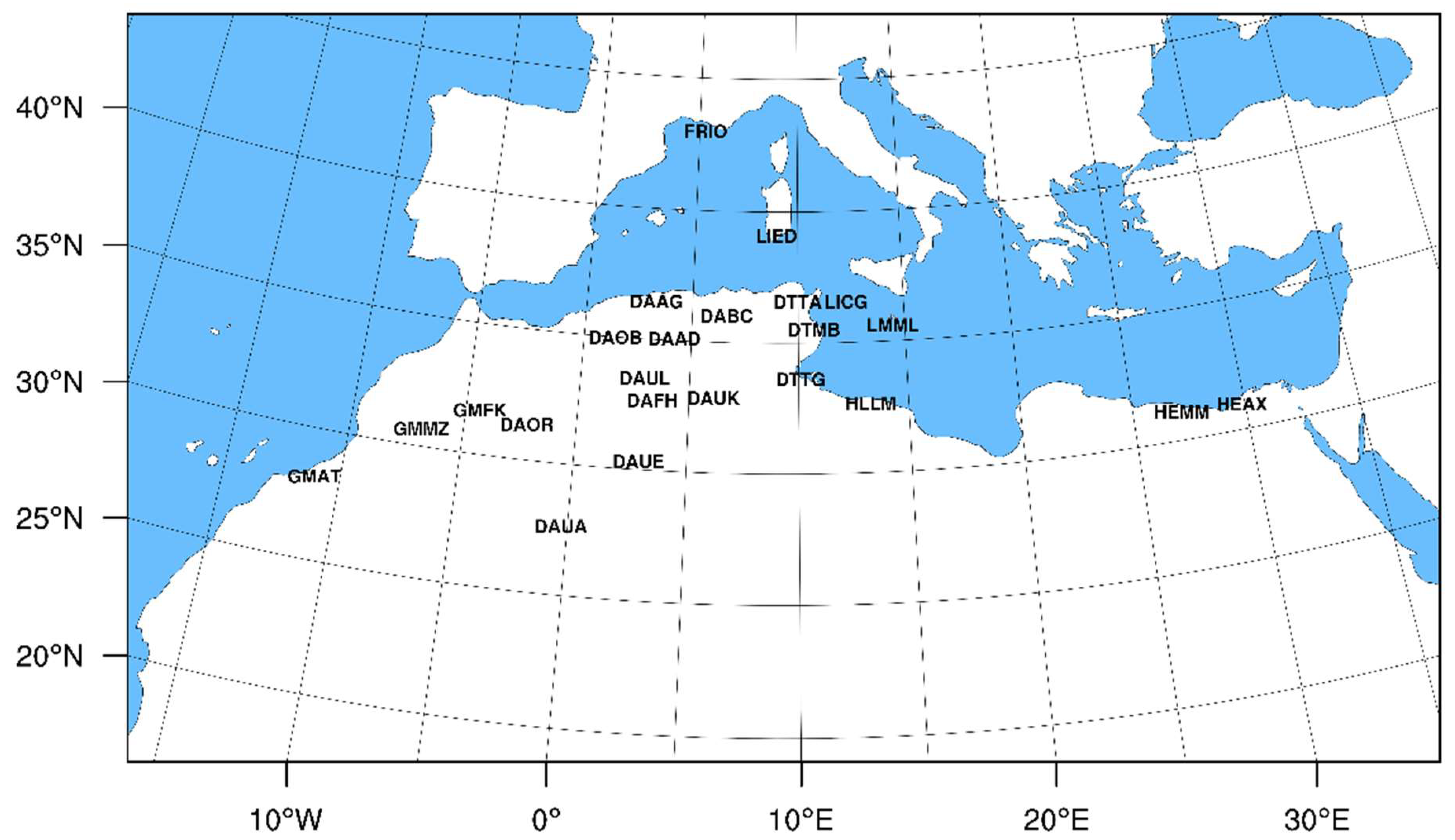
2.2. Global Surface Observational Dataset

Surface observations of hourly wind speed and temperature from 1 to 30 November 2017 at 23 meteorological stations were used. Figure 1 shows the location of the meteorological aviation reporting (METAR) (excluding FRIO) stations in the simulated domain with acronyms by the International Civil Aviation Organization, while the coordinates (lat, lon, elev) are reported in

Table 3. Acronym and position (lat, lon, elev) of the meteorological aviation reporting (METAR) stations.

Stations in the Northern Sahara	Country	ICAO Station Name	Latitude	Longitude	Altitude (m)
Bou Saada	Algeria	DAAD	35.33 N	4.20 E	461
Dar El Beida Houari	Algeria	DAAG	36.72 N	3.25 E	25
Constantine El Bey	Algeria	DABC	36.28 N	6.62 E	694
Tilrempt Hassi	Algeria	DAFH	32.93 N	3.32 E	774
Tiaret	Algeria	DAOB	35.25 N	1.43 E	1127
Bechar Ouakda	Algeria	DAOR	31.62 N	2.23 W	773
Adrar Touat	Algeria	DAUA	27.88 N	0.28 W	263
El Golea	Algeria	DAUE	30.57 N	2.87 E	397
Touggourt Sidi Mahd	Algeria	DAUK	33.12 N	6.13 E	85
Laghouat	Algeria	DAUL	33.77 N	2.93 E	765
Habib Bourguiba	Tunisia	DTMB	35.77 N	10.75 E	2
Tunis Carthage	Tunisia	DTTA	36.83 N	10.23 E	4
Gabes	Tunisia	DTTG	33.88 N	10.10 E	5
Tan-Tan Civ Mil	Morocco	GMAT	28.43 N	11.15 W	200
Er Rachidia Rma	Morocco	GMFK	31.95 N	4.40 W	1045
Ouarzazate	Morocco	GMMZ	30.92 N	6.90 W	1140
Alexandria	Egypt	HEAX	31.20 N	29.95 E	7
Mersa Matruh	Egypt	HEMM	31.33 N	27.22 E	30
Tripoli Mitiga	Libya	HLLM	32.89 N	13.28 E	11
Stations in the Mediterranean basin
Pantelleria	Italy	LICG	36.82 N	11.97 E	191
Decimomannu	Italy	LIED	39.35 N	8.97 E	28
Luqa	Malta	LMML	38.85 N	14.48 E	91
Frioul	France	FRIO	43.26 N	5.29 E	40

ICAO—International Civil Aviation Organization.

. Source areas of Saharan dust located between Algeria and Tunisia contribute to dust outbreak episodes over the Mediterranean basin [37,38,39]. Therefore, 13 of the 19 weather stations in Northern Africa considered in the present study are located between Algeria and Tunisia (Table 3).

Apart from the data of the FRIO meteorological station, which were provided by the Mediterranean Institute of Oceanography of the University of Toulon (https://www.mio.univ-amu.fr/?lang=en), all the measurement data were obtained from the University of Wyoming web site (http://weather.uwyo.edu/index.shtml). These weather stations utilize the World Meteorological Organization-approved METAR format, which is a standard common format for reporting weather information for aviation meteorology every 30 min or 1 h.

2.3. The Statistical Method for the Model Performance Evaluation

The model performance evaluation [40] of WRF was assessed comparing the simulated 10 m wind speed and 2 m temperature with observational data. A set of four statistical indexes, i.e., the mean bias (MB), the mean absolute error (MAE), the root mean square error (RMSE), and the correlation coefficient (COR), were estimated for simulated and observational values according to the equations in

Table A1. Statistical indexes formulas for predicted (pred) and observed (obs) values.

$MB=\frac{{{\displaystyle \sum }}_{\mathrm{i}=1}^{\mathrm{n}}\left({\mathrm{X}}_{\mathrm{i}-\mathrm{pred}}-{\mathrm{X}}_{\mathrm{i}-\mathrm{obs}}\right)}{n}$

$MAE=\frac{{{\displaystyle \sum }}_{\mathrm{i}=1}^{\mathrm{n}}{|\mathrm{X}}_{\mathrm{i}-\mathrm{pred}}-{\mathrm{X}}_{\mathrm{i}-\mathrm{obs}}|}{n}$

$RMSE=\sqrt{\frac{{{\displaystyle \sum }}_{\mathrm{i}=1}^{\mathrm{n}}{\left({\mathrm{X}}_{\mathrm{i}-\mathrm{pred}}-{\mathrm{X}}_{\mathrm{i}-\mathrm{obs}}\right)}^2}{n}}$

$COR=\frac{{{\displaystyle \sum }}_{i=1}^n\left({\mathrm{X}}_{\mathrm{i}-\mathrm{pred}}-{\overline{X}}_{pred}\right)\left({\mathrm{X}}_{\mathrm{i}-\mathrm{obs}}-{\overline{X}}_{obs}\right)}{\sqrt{{{\displaystyle \sum }}_{i=1}^n{\left({\mathrm{X}}_{\mathrm{i}-\mathrm{pred}}-{\overline{X}}_{pred}\right)}^2 {\left({\mathrm{X}}_{\mathrm{i}-\mathrm{obs}}-{\overline{X}}_{obs}\right)}^2} }$

MB—mean bias; MAE—mean absolute error; RMSE—root mean square error; COR—correlation coefficient.

. In addition, for selected stations, a direct comparison between time series model outputs and observational data is shown. Finally, to make a synthesis of all results, the Taylor diagrams [41] are depicted.

3. Results and Discussion

3.1. Analysis of the Model Output for the Northern Sahara

First, the results are presented as overall statistics of all the meteorological stations located in the Northern Sahara and listed in Table 3. Then, the three METAR stations that may be considered as the most representative of the dust area sources are discussed in detail.

3.1.1. Overall Statistics

In

Table 4. Summary of the overall statistics between predicted and measured 2 m temperature at meteorological aviation reporting (METAR) stations in the Northern Sahara.

Runs	MB (K)	MAE (K)	RMSE (K)	COR
MY	0.11	2.33	9.80	0.87
NOAH	0.88	2.28	9.70	0.86
RU	0.52	2.37	10.32	0.86
MY1	0.14	2.33	9.81	0.87
N0	−0.27	2.12	8.51	0.89
N1	−0.32	2.14	8.64	0.89
N2	−0.46	2.27	9.36	0.89
N3	−0.47	2.24	9.31	0.89

MB—mean bias; MAE—mean absolute error; RMSE—root mean squared error; COR—correlation coefficient.

, we have reported the overall statistics calculated considering the 2 m temperature for the whole set of Sahara METAR stations. In terms of MB, a remarkable distinction is evident between runs with and without nudging. The positive mean biases (up to 0.88 K) indicate an overestimation of the predicted 2 m temperature for the simulations with no nudging (MY, NOAH, RU, and MY1), whereas the negative mean biases (up to 0.47 K) identify an underestimation of the predicted surface temperature for the simulations with nudging (N0, N1, N2, and N3). In terms of MAE and COR, there are no substantial differences between the simulations, since the values are in the ranges [2.12–2.37] K and [0.86–0.89], respectively, although the nudging simulations appear more skillful. The most remarkable difference is evident when considering the RMSE, for which the simulations with nudging (N0-N3) show lower values, with the lowest RSME value of 8.51 K in N0.

Other important considerations can be drawn: (i) the comparison between the MY and MY1 temperature statistics (Table 4) suggests no substantial differences by switching from MODIS to USGS land use dataset for WPS preprocessing; (ii) NOAH (sf_surface_physics = 4) is slightly better compared to RUC (sf_surface_physics = 3) (lower RMSE), but has higher MB; (iii) as surface layer physics, the MYNN [27] similarity scheme (MY) performs slightly better than the MM5 similarity [31] scheme (RU) in predicting 2 m temperature. The overall statistical analysis of the model runs shows that the nudged run (N0) is the best model configuration for predicting surface temperature in the Northern Sahara, having the highest COR (0.89) and the lowest temperature MAE (2.12 K) and RMSE (8.51 K).

The overall statistical analysis for the 10 m wind speed is depicted in

Table 5. Summary of the statistics between predicted and measured 10 m wind speed at meteorological aviation reporting (METAR) stations in the Northern Sahara.

Runs	MB (m s−1)	MAE (m s−1)	RMSE (m s−1)	COR
MY	−0.18	1.58	4.82	0.51
NOAH	0.92	1.92	7.02	0.52
RU	−0.06	1.60	4.99	0.48
MY1	0.12	1.65	5.27	0.51
N0	−0.03	1.51	4.45	0.59
N1	−0.08	1.46	4.23	0.61
N2	−0.46	1.42	3.94	0.64
N3	−0.51	1.46	4.08	0.64

MB—mean bias; MAE—mean absolute error; RMSE—root mean squared error; COR—correlation coefficient.

. One may identify a larger variation (between min and max) of the statistical parameters compared to the temperature. Again, in terms of MB, a little underestimation of the predicted surface wind speed is evident for the simulations with nudging (i.e., N0, N1, N2, and N3) while the greatest overestimation occurs for the NOAH run with MB = 0.92 m s⁻¹. The better performance of the runs with nudging is apparent when considering MAE and RMSE and the correlation.

Like for Table 4, similar considerations may be drawn analyzing Table 5: (i) little differences are observed between the MY and MY1 runs for all statistical indexes, with better results for the MY case (MODIS IGBP 21-category); (ii) NOAH run gives the overall worst results; (iii) the predicted wind speeds, from the different model runs with nudging, have higher correlations with the observations compared to the model setups with no nudging, with COR values in the range of 0.59–0.64 (down to 0.48 for the models without nudging). The highest COR (0.64) and the lowest wind speed MAE (1.42 m s⁻¹) and RMSE (3.94 m s⁻¹) suggest that the nudged run with N2-setup is the recommended configuration for predicting surface wind speed in the Northern Sahara.

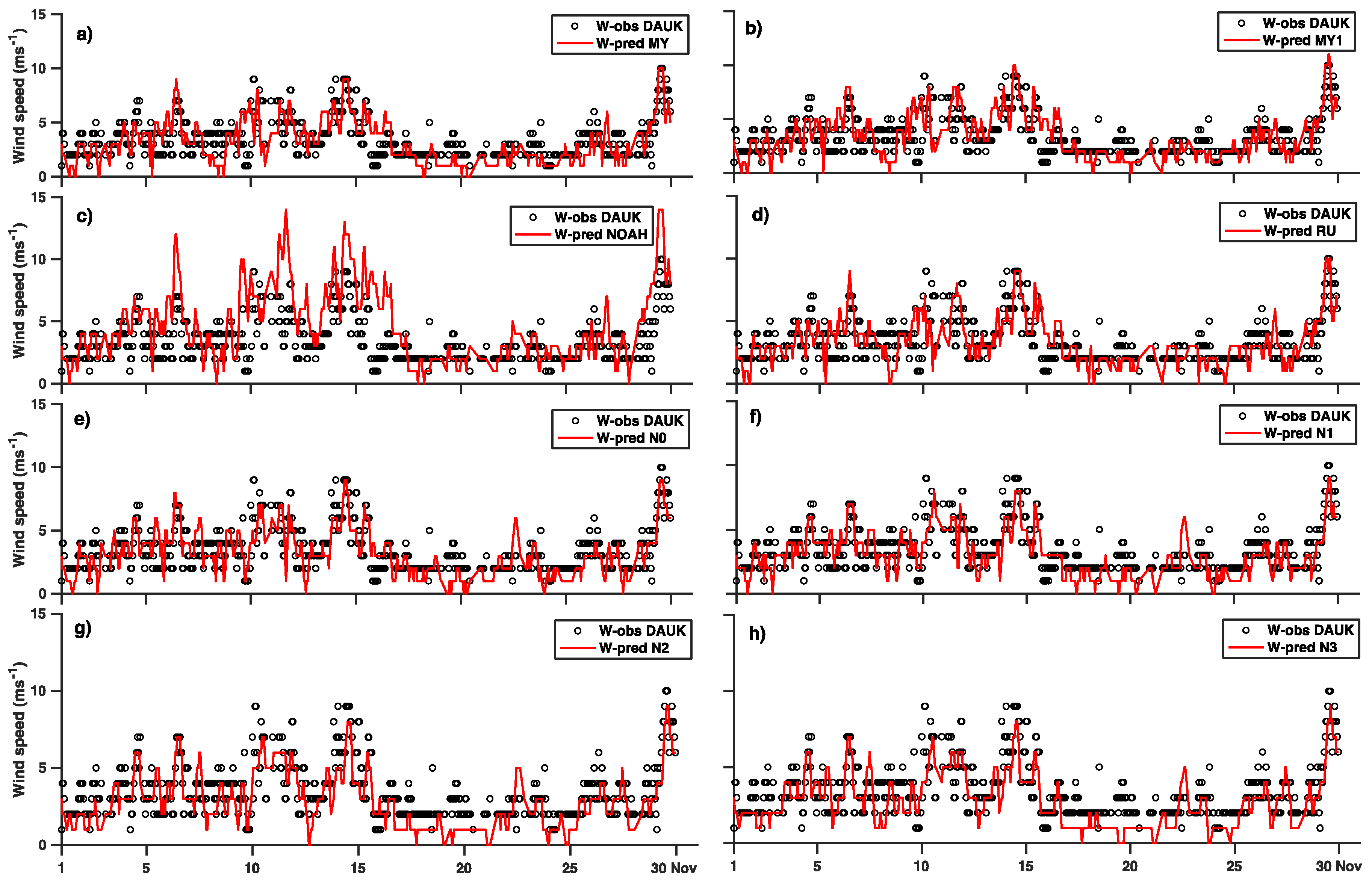
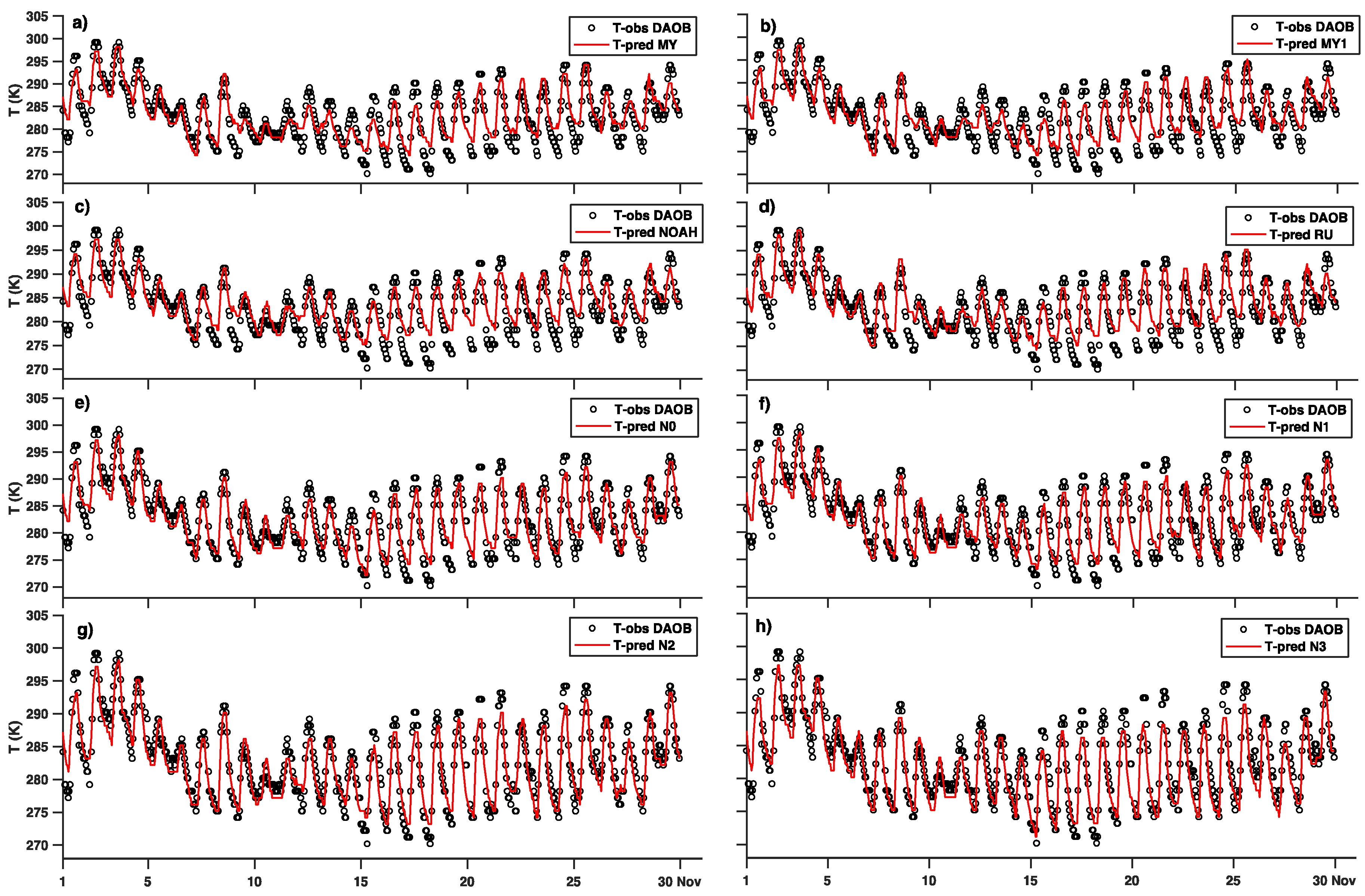
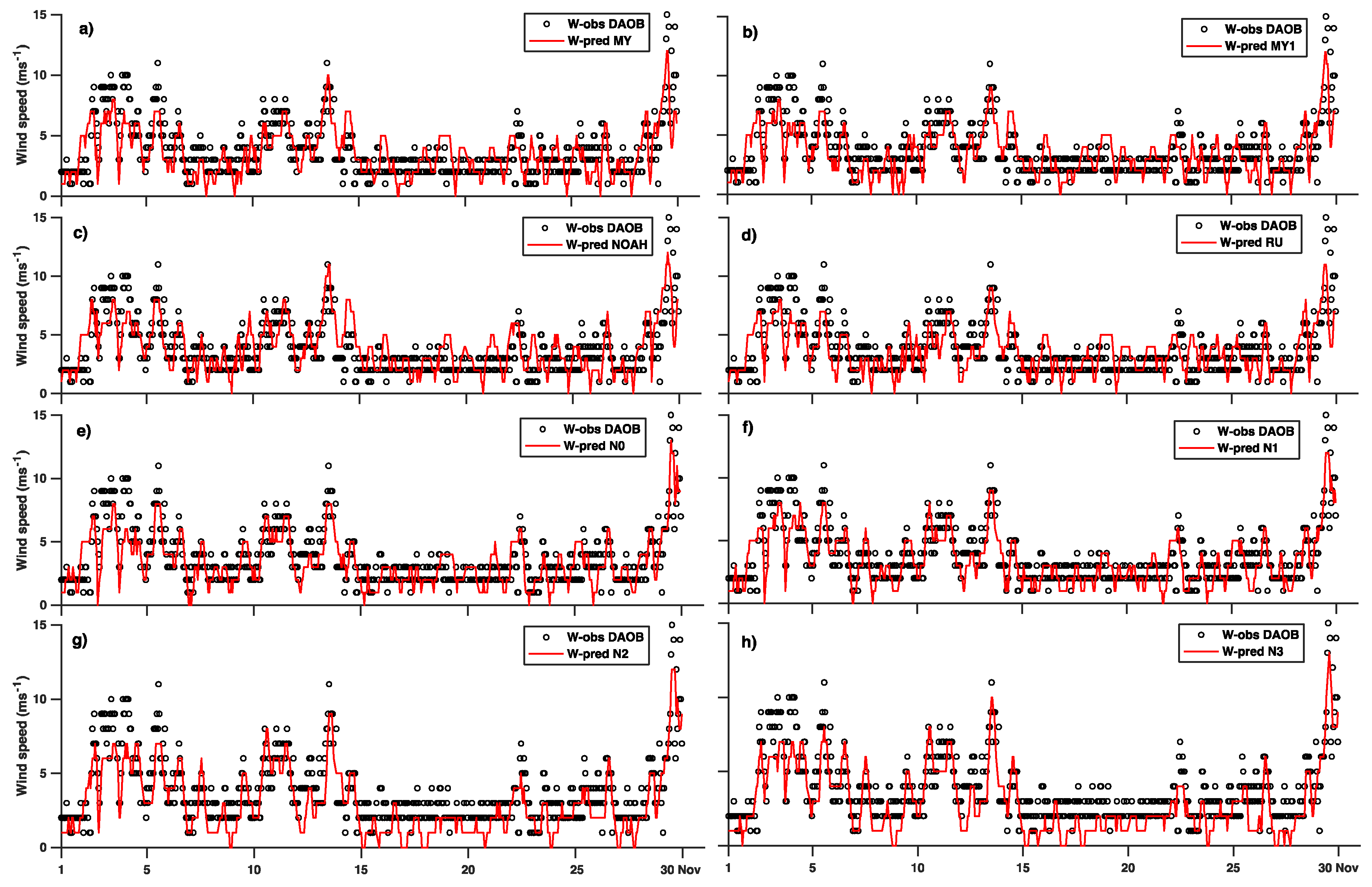
3.1.2. Time Series and Statistical Analysis on Selected Stations

Further insights are given analyzing the time series and statistics of 2 m temperature and 10 m wind speed in three METAR stations that may be considered as representative of the dust area sources. The selected METAR stations (DTMB, DAUK, and DAOB) are located in the northern region of Sahara Desert (Figure 1 and Table 3), between the Atlas Mountains (DAOB) and the coast of Tunisia (DTMB), while DAUK is located in an internal desert area of Algeria.

Figure 2 shows the time series of the predicted 2 m temperature (red continuous line) compared with the respective measurements (black circles).The time series span the whole month of November 2017, and each panel refers to each configuration as described in the legend.

Since DTMB is a coastal station, it may be subject to local circulation systems not properly resolved by a 20 km grid. The daily–night temperature cycle is well reproduced by all simulations with the best results for the nudged runs. In particular, the run N3 gives the best statistics in this station as can be seen in

Table A2. Mean absolute error (MAE), root mean square error (RMSE), and correlation coefficient (COR) for surface temperature (Temp) at Habib Bourguiba (Tunisia); meteorological aviation reporting (METAR) station code = DTMB.

Temp-DTMB	MAE (K)	RMSE (K)	COR
RU	1.90	6.21	0.86
NO	1.62	4.64	0.86
MY	1.84	5.48	0.87
MY1	1.90	5.78	0.87
N0	1.83	4.96	0.92
N1	1.82	4.92	0.91
N2	2.03	5.87	0.91
N3	1.39	3.24	0.91

(Appendix A).

These results are confirmed by analyzing the 10 m wind speed in Figure 3. It is evident how the introduction of the nudging produces a better modulation of the 10 m wind speed (in particular N3), especially for the maximum values, as confirmed by statistical indexes reported in

Table A3. Mean absolute error (MAE), root mean square error (RMSE), and correlation coefficient (COR) for surface wind at Habib Bourguiba (Tunisia); meteorological aviation reporting (METAR) station code = DTMB.

wind-DTMB	MAE (m s−1)	RMSE (m s−1)	COR
RU	1.88	8.03	0.43
NO	1.88	7.38	0.54
MY	1.73	6.41	0.58
MY1	1.73	6.48	0.57
N0	1.35	4.04	0.77
N1	1.32	3.96	0.77
N2	1.29	3.73	0.79
N3	1.27	3.63	0.78

(Appendix A).

Figure 4 shows the 2 m temperature comparison at DAUK station in an internal region of Algeria (Table 3). Again, the day/night temperature oscillations are well reproduced, especially by the nudged runs, and the best results are obtained for N3 as shown in

Table A4. Mean absolute error (MAE), root mean square error (RMSE), and correlation coefficient (COR) for surface temperature (Temp) at Touggourt Sidi Mahd (Algeria); meteorological aviation reporting (METAR) station code = DAUK.

Temp-DAUK	MAE (K)	RMSE (K)	COR
RU	2.14	7.72	0.93
NO	2.47	9.16	0.92
MY	1.82	5.96	0.93
MY1	1.88	6.26	0.93
N0	1.37	3.50	0.95
N1	1.35	3.54	0.95
N2	1.51	4.02	0.95
N3	1.32	3.22	0.94

(Appendix A).

The 10 m wind speed at DAUK is shown in Figure 5. In the second part of the month, the measured data present many periods with constant, low wind speed (at around 2 m s⁻¹), indicating anticyclonic conditions with weak pressure gradients. As depicted in

Table A5. Mean absolute error (MAE), root mean square error (RMSE), and correlation coefficient (COR) for surface wind at Touggourt Sidi Mahd (Algeria); meteorological aviation reporting (METAR) station code = DAUK.

wind-DAUK	MAE (m s−1)	RMSE (m s−1)	COR
RU	1.27	2.77	0.60
NO	1.96	7.11	0.64
MY	1.30	2.82	0.62
MY1	1.32	2.90	0.64
N0	1.08	1.88	0.72
N1	1.03	1.72	0.75
N2	1.11	1.91	0.76
N3	1.11	1.96	0.75

(Appendix A), the best results are for the nudging configuration N2.

Finally, in Figure 6 and Figure 7, we have reported the comparison of temperature and wind speed for DAOB station, which is located in the Atlas Mountains at 1127 m above sea level (Table 3). Diurnal excursions are very high since measured temperatures reach 0 °C at night and 25 °C during the day (Figure 6). This behavior is only reproduced by the nudged runs, with the best statistical results again from N2 configurations (

Table A6. Mean absolute error (MAE), root mean square error (RMSE), and correlation coefficient (COR) for surface temperature (Temp) at Tiaret (Algeria); meteorological aviation reporting (METAR) station code = DAOB.

Temp-DAOB	MAE (K)	RMSE (K)	COR
RU	2.05	6.47	0.92
NO	2.21	7.56	0.92
MY	2.18	6.84	0.91
MY1	2.17	6.81	0.91
N0	1.67	4.09	0.95
N1	1.64	3.92	0.95
N2	1.51	3.43	0.96
N3	1.67	4.43	0.96

Appendix A). The improvement is remarkable for both runs N2 and N3 (Figure 6).

The wind speed statistical analysis shown in

Table A7. Mean absolute error (MAE), root mean square error (RMSE), and correlation coefficient (COR) for surface wind at Tiaret (Algeria); meteorological aviation reporting (METAR)station code = DAOB.

wind-DAOB	MAE (m s−1)	RMSE (m s−1)	COR
RU	1.39	3.23	0.66
NO	1.40	3.30	0.67
MY	1.38	3.02	0.69
MY1	1.40	3.12	0.68
N0	1.20	2.48	0.76
N1	1.17	2.29	0.78
N2	1.27	2.50	0.81
N3	1.28	2.52	0.83

in Appendix A and in Figure 7 again confirms N2 as the best configuration. It is important to point out in Figure 7 that during the first week of the month, all simulations underestimate the wind speed while the comparison improves in the rest of the month.

3.2. Analysis of the Model Output for the Mediterranean Basin

First, the results are presented as overall statistics over all the meteorological stations located in the Mediterranean basin and listed in Table 3. Then, the results for each station in the Mediterranean basin are discussed in detail.

3.2.1. Overall Statistics

In

Table 6. Summary of the statistics between predicted and measured 2 m temperature at meteorological stations in the Mediterranean basin.

Runs	MB (K)	MAE (K)	RMSE (K)	COR
MY	0.68	1.76	5.01	0.82
NOAH	1.05	1.72	5.52	0.82
RU	0.89	1.83	5.42	0.81
MY1	0.74	1.82	5.20	0.82
N0	0.68	1.74	4.74	0.85
N1	0.72	1.73	4.74	0.84
N2	0.52	1.67	4.72	0.84
N3	0.62	1.54	3.85	0.89

MB—mean bias; MAE—mean absolute error; RMSE—root mean squared error; COR—correlation coefficient.

we have reported the overall statistics calculated considering the 2 m temperature measured at the three METAR stations (LICG, LIED and LMML) and the University of Toulon station denoted as FRIO in Table 3.

The analysis of Table 6 shows that the nudged runs (N0-N3) provide the overall best results for all statistical indexes. It is evident that the gradual inclusion of nudging improves the model performances. The MAE is reduced from 1.82 K of the MY1 run and to 1.54 K of the N3 run; analogously, the RMSE changes from 5.20 K (MY1) to 3.85 K (N3); and finally, the correlation coefficient increases from 82% (MY1) to 89% (N3).

Other considerations can be drawn: (i) comparisons between the MY and MY1 temperature statistics show no substantial differences when switching from MODIS to USGS land use WPS categories; (ii) the two surface layer schemes—that is the MM5 similarity scheme (RU) and the MYNN scheme (MY)—perform quite similarly in predicting 2 m temperature with the employed model set up with the MAE and RMSE of the RU case slightly higher than MY.

A remarkable conclusion is that the gradual introduction of nudging parameters from N0 to N3 run leads to lower-temperature MAE and RMSE compared to the reference case with no nudging (i.e., MY1) by 4.4–15.4% and 8.8–26%, respectively. Thus, N3 is the best model setup for predicting 2 m temperature in the Mediterranean basin, having the highest COR (0.89) and the lowest MAE (1.54 K) and RMSE (3.85 K).

Considering the overall statistics for the 10 m wind speed (

Table 7. Summary of the statistics between predicted and measured 10 m wind speed at meteorological stations in the Mediterranean basin.

Runs	MB (m s−1)	MAE (m s−1)	RMSE (m s−1)	COR
MY	−0.01	1.79	6.31	0.71
NOAH	0.68	2.02	7.32	0.68
RU	0.72	2.03	7.79	0.68
MY1	0.12	1.82	6.18	0.70
N0	−0.13	1.59	4.79	0.77
N1	−0.04	1.61	4.78	0.77
N2	0.00	1.66	5.02	0.78
N3	0.05	1.65	4.93	0.78

MB—mean bias; MAE—mean absolute error; RMSE—root mean squared error; COR—correlation coefficient.

), similar considerations may be drawn, as it is still evident that the inclusion of nudging improves in a robust way all the statistical indices. In particular, MAE is reduced from 1.82 m s⁻¹ of the MY1 run to 1.61 m s⁻¹ of the N1 run; analogously, RMSE passes from 6.18 m s⁻¹ (MY1) to 4.78 m s⁻¹ (N1); finally, the correlation coefficient increases from 0.70 (MY1) to 0.78 (N1).

No substantial differences are observed comparing the 10 m wind statistics between the NOAH and RU case and between the MY and MY1 case (Table 7). Therefore, employing either of the two LSMs (i.e., Noah-MP and RUC) and land use datasets (i.e., USGS and MODIS) is almost the same for predicting 10 m wind speed in the Mediterranean basin considering the above-mentioned model configurations.

As a surface layer scheme, the MYNN scheme performs better than the MM5 similarity scheme in predicting 10 m wind speed with the selected model set up, with the MAE and RMSE of the MY run lower than the RU case by 0.24 and 1.48 m s⁻¹, respectively.

N0 and N1 are the best model setups for predicting 10 m wind speed in the Mediterranean basin, having the lowest wind speed MAE (up to 1.61 m s⁻¹) and RMSE (up to 4.79 m s⁻¹). Introducing the nudging of horizontal wind speed in the PBL (i.e., N2 run) and total nudging (i.e., N3 run) leads to no substantial changes, with wind speed MAE and RMSE higher than the N0 and N1 runs by up to 0.07 and 0.24 m s⁻¹.

The predicted temperature and wind speed from the different model runs with nudging have slightly higher correlations with the observations compared to the ones with no nudging, with COR values in the range of 0.83–0.89 for the runs with nudging versus 0.77–0.82 for the ones with no nudging. Therefore, introducing nudging parameters leads to an overall improvement of the predicted surface temperature and wind speed in the Mediterranean basin for the model configurations that have been tested here.

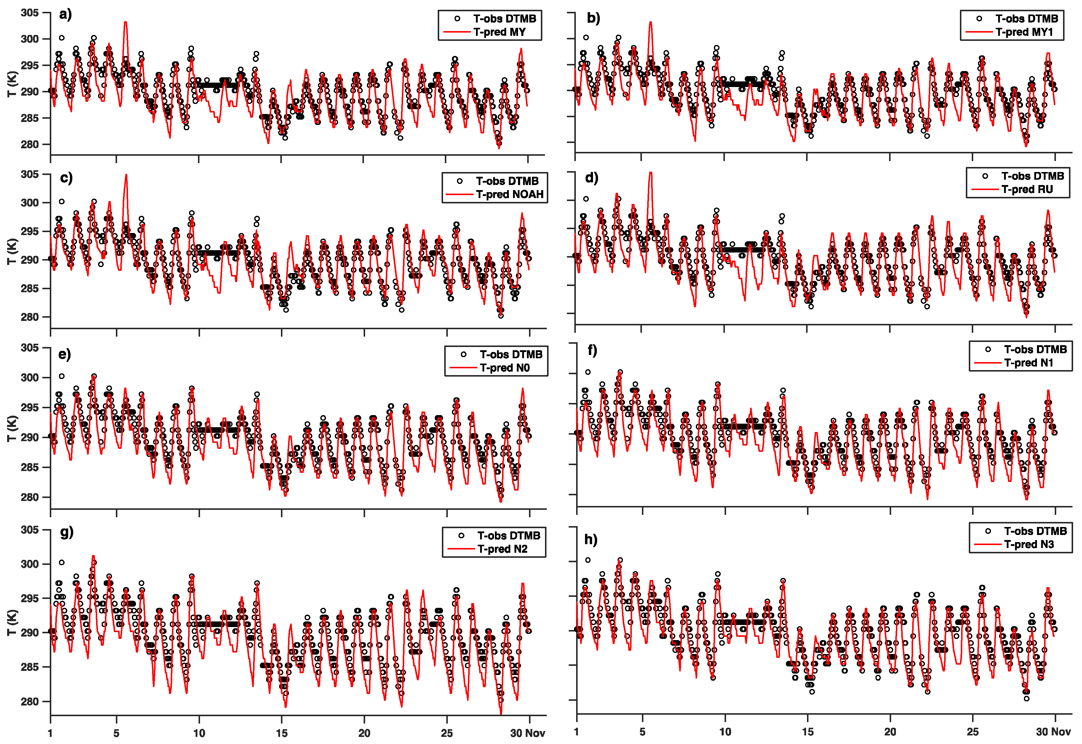
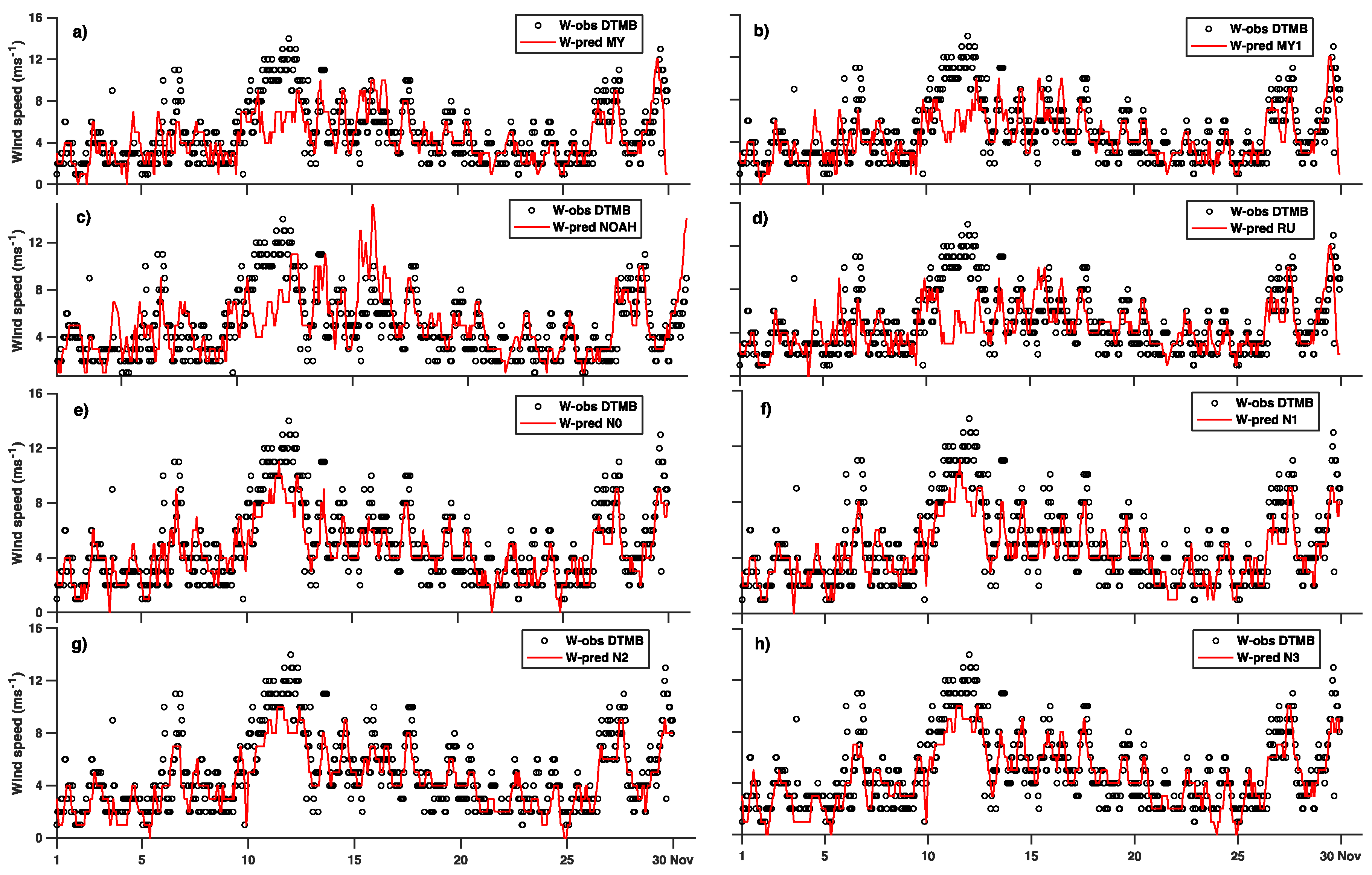
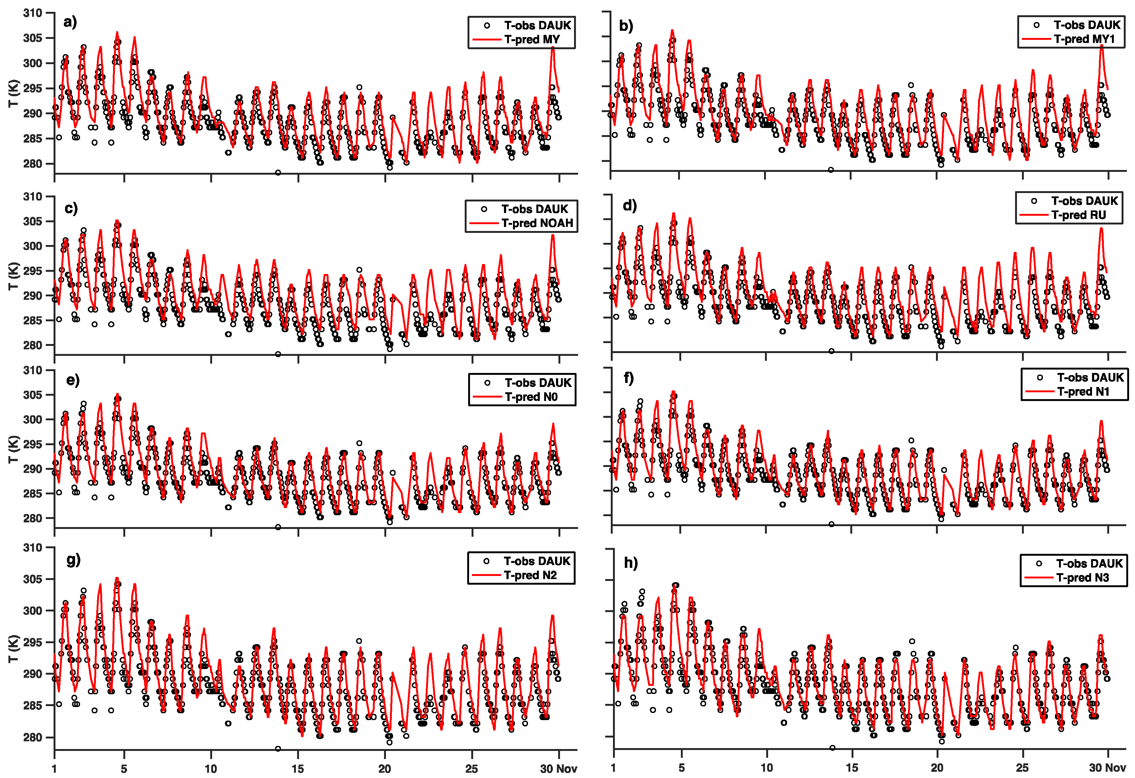
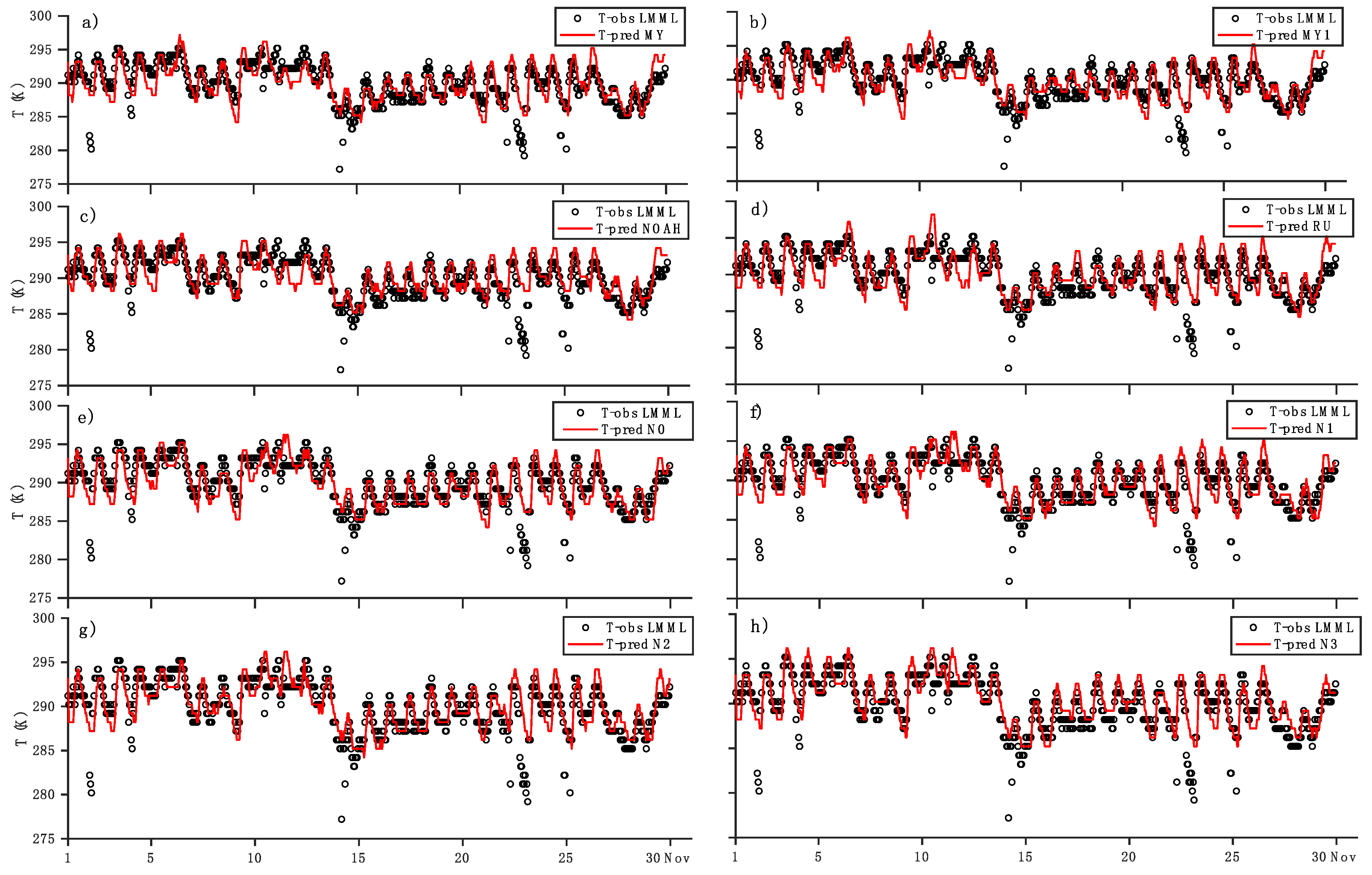
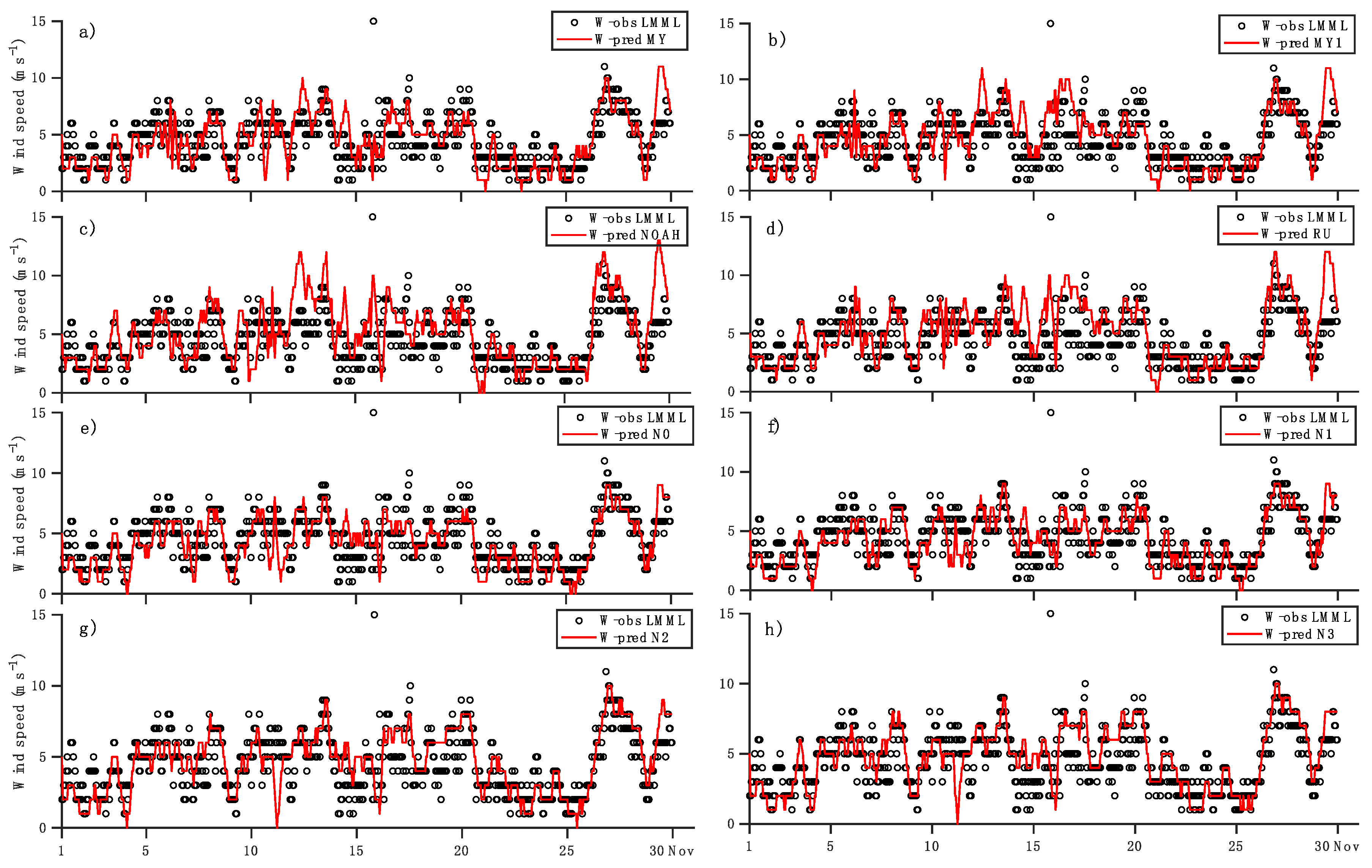
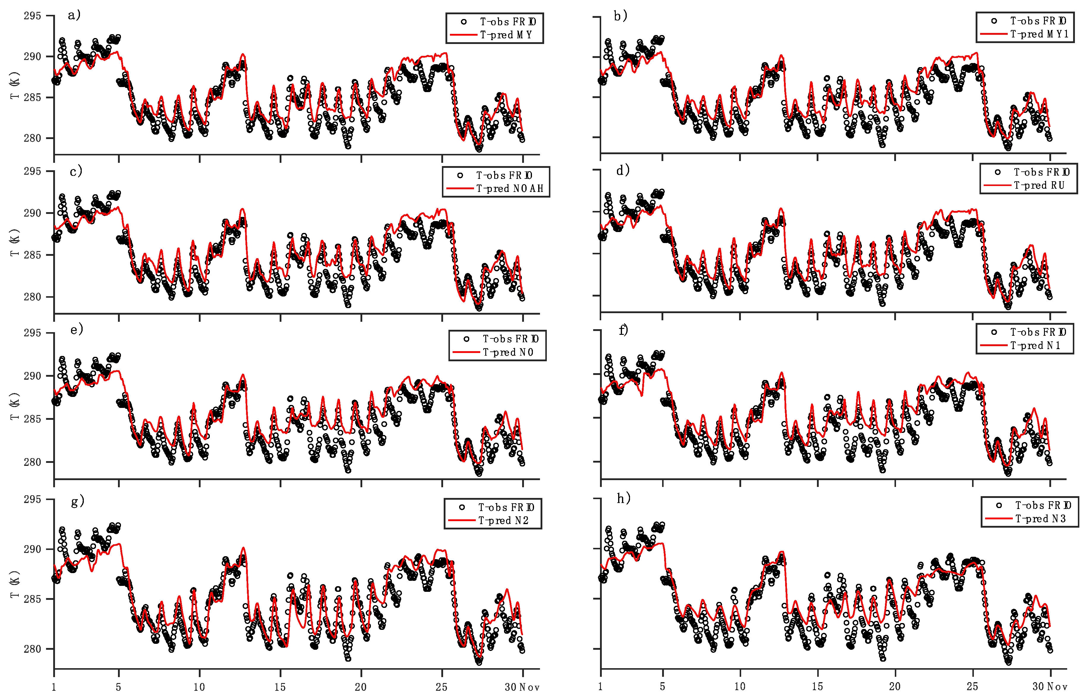
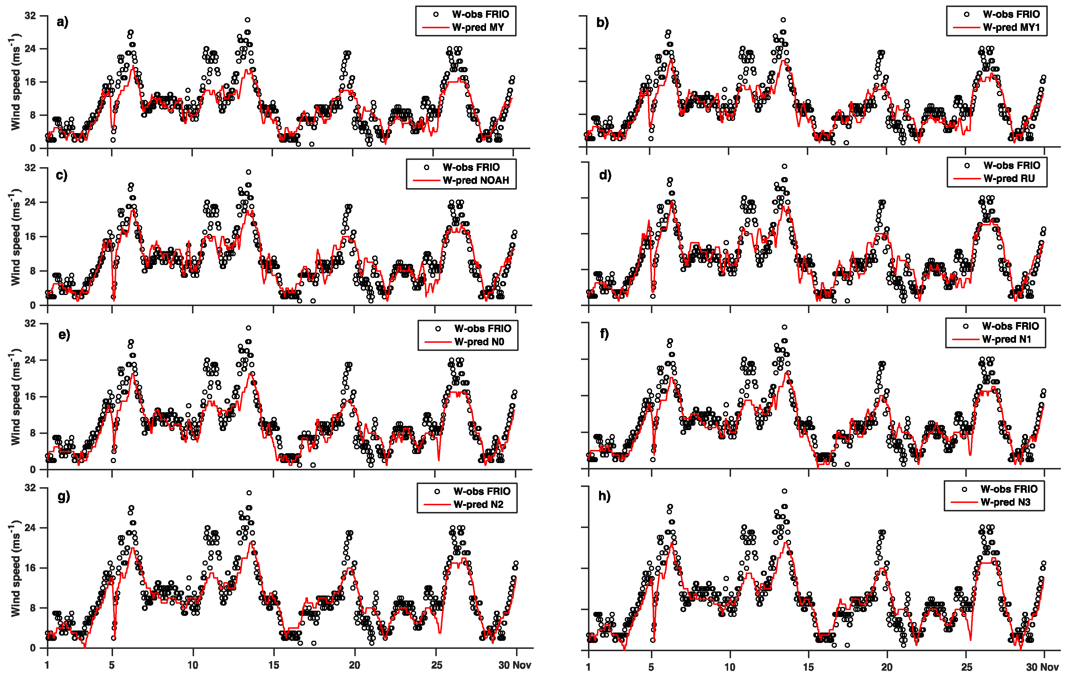
3.2.2. Time Series and Statistical Analysis on Selected Stations

Further insights may be obtained analyzing the time-series and the statistics of two specific surface stations in the Mediterranean basin. The first station that is considered is localized at Luqa Malta (METAR code LMML).

Figure 8 shows the temporal evolution of measured and modeled 2 m temperature. A reduced night/day variation typical of maritime conditions is apparent. This behavior is reproduced pretty well by all configurations, especially by the nudged run N3, and well represented in the statistical analysis depicted at

Table A8. Mean absolute error (MAE), root mean square error (RMSE), and correlation coefficient (COR) for surface temperature (Temp) at Luqa (Malta); meteorological aviation reporting (METAR) station code = LMML.

Temp-LMML	MAE (K)	RMSE (K)	COR
RU	1.48	4.14	0.75
NO	1.35	3.75	0.77
MY	1.43	3.68	0.77
MY1	1.42	3.59	0.78
N0	1.36	3.30	0.80
N1	1.32	3.38	0.79
N2	1.27	3.30	0.80
N3	1.21	2.77	0.84

in Appendix A. Some cold outbreaks are not reproduced in any configurations; this is probably a consequence of the coarse resolution that does not allow one to properly resolve the small island.

The wind speed is shown in Figure 9. Maximum values are much better reproduced by nudged runs, as confirmed by statistical analysis in

Table A9. Mean absolute error (MAE), root mean square error (RMSE), and correlation coefficient (COR) for surface wind at Luqa (Malta); meteorological aviation reporting (METAR) station code = LMML.

wind-LMML	MAE (m s−1)	RMSE (m s−1)	COR
RU	1.51	4.07	0.66
NO	1.60	4.53	0.66
MY	1.25	2.69	0.72
MY1	1.37	3.31	0.69
N0	1.13	2.25	0.74
N1	1.07	2.07	0.76
N2	1.10	2.28	0.74
N3	1.13	2.40	0.74

in Appendix A.

The other station analyzed in this Section is placed at the Island of Frioul, few kilometers offshore Marseille in southern France. Data are provided by the Mediterranean Institute of Oceanography of the University of Toulon.

Time evolution of 2 m temperature (Figure 10) is very well reproduced by all configurations except for the third week of the month, where only the N2 run is able to reproduce the day/night variation, as confirmed by the statistical analysis reported in

Table A10. Mean absolute error (MAE), root mean square error (RMSE), and correlation coefficient (COR) for surface temperature (Temp) at Frioul (France) station denoted as FRIO.

Temp-FRIO	MAE (K)	RMSE (K)	COR
RU	1.30	2.55	0.92
NO	1.30	2.56	0.91
MY	1.24	2.35	0.92
MY1	1.42	2.98	0.91
N0	1.39	3.00	0.91
N1	1.41	3.09	0.90
N2	1.10	2.21	0.90
N3	1.22	2.38	0.93

in Appendix A, RMSE in particular.This result supports the idea that the best results from grid-nudging are obtained when (T, Q) are not nudged within the PBL [35,42,43], as it is the case with the N2 run.

The wind speed is shown in Figure 11. It is remarkable that in November 2017, at least five events occurred with wind speed greater than 24 m s⁻¹, with a peak of 31 m s⁻¹ in the second week. All the configurations provide good results, but it does not seem that the nudged runs are able to improve the reproduction of the peaks. Under these severe wind conditions (112 km h⁻¹), in the WRF model, the isftcflx option should be activated, which provides alternative surface-layer options for high-wind ocean surface, as discussed by Green and Zhang [44].

Table A11. Mean absolute error (MAE), root mean square error (RMSE), and correlation coefficient (COR) for surface wind at Frioul (France) station denoted as FRIO.

wind-FRIO	MAE (m s−1)	RMSE (m s−1)	COR
RU	2.37	10.00	0.86
NO	2.39	10.12	0.86
MY	2.55	12.46	0.87
MY1	2.46	11.08	0.87
N0	2.30	9.87	0.89
N1	2.26	9.52	0.90
N2	2.27	9.31	0.90
N3	2.21	8.90	0.90

in Appendix A shows anyway that, like in many other cases, the N3 run produced the best statistics for the whole month.

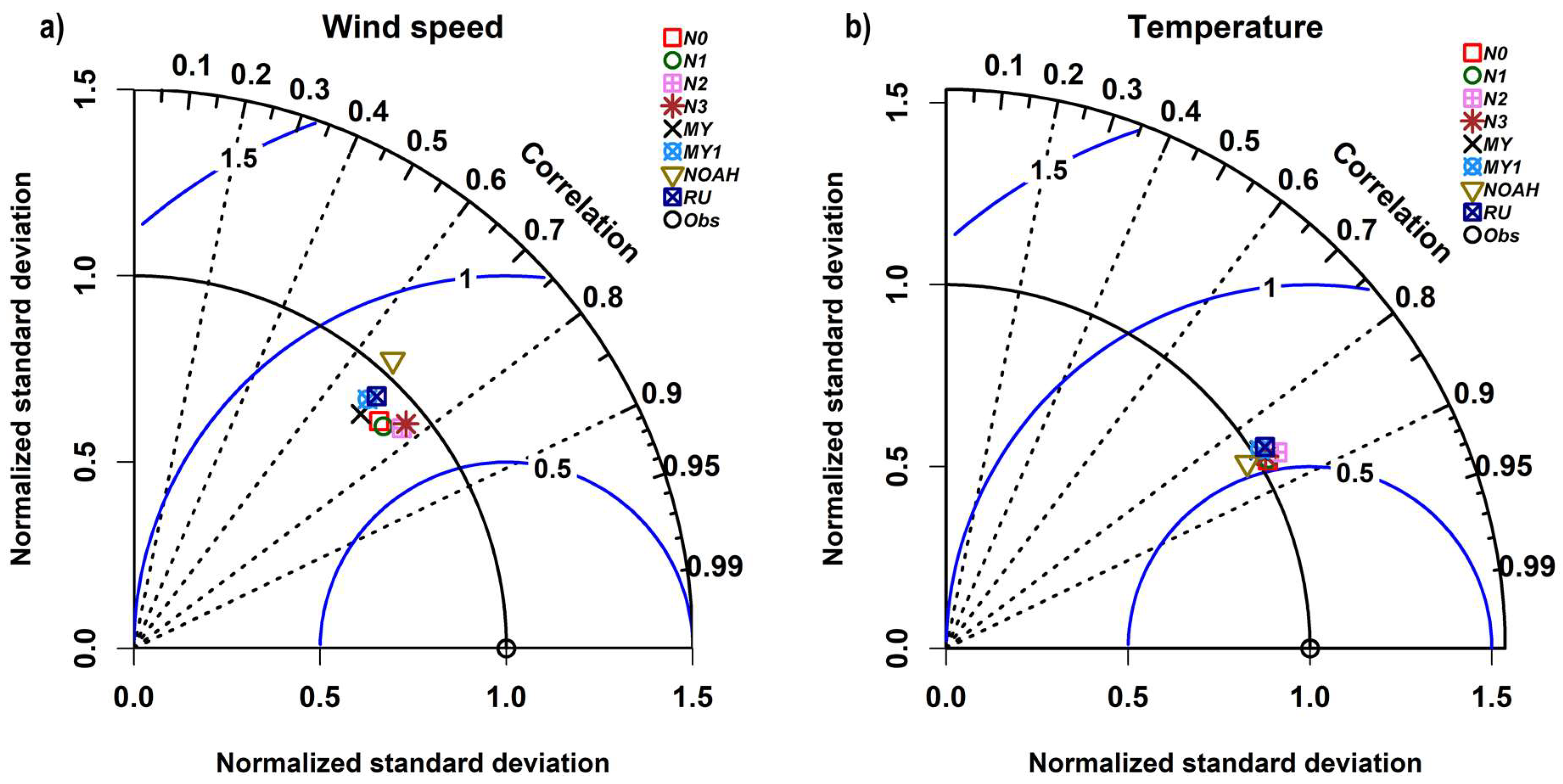
3.3. Global Statistics

To make a synthesis of the results, we have depicted the Taylor diagrams [41] for wind speed (Figure 12a) and temperature (Figure 12b). These diagrams have been calculated considering the whole experimental dataset and may be considered as a synthesis of the global results. Figure 12a provides a summary of the relative skill of different model setups in the simulation of the spatial pattern of mean wind speed. The azimuthal angle represents the Pearson correlation coefficient, for which it is evident that the configurations (with nudging) N2 and N3 give the best results. The same considerations may be reported for the centered RMSE (distance from blue lines).

Figure 12b shows a summary of the global temperature statistics. It is evident that in this case, the Taylor diagram reports a minor scatter between all model configurations with the best results for the N0 setup, confirming the considerations reported above.

4. Conclusions

This paper aims at analyzing the optimal configuration for the WRF model in reproducing the wind speed and temperature fields in a numerical domain that includes the Northern Sahara and the Mediterranean basin. This is important for the assessment of the emissions of mineral dust and sea spray in the Mediterranean region.

A series of simulations for the whole month of November 2017 was performed with the WRF model, version 3.9.1. Eight different setups were considered, the first four reflecting different combinations of the physical parameters describing the surface layer scheme and the land surface model, and the last four representing different arrangements of the nudging parameters. The model results were compared with the near-surface temperature and wind speed data downloaded from the global surface observational dataset available at the University of Wyoming web portal, and with an additional dataset provided by the Mediterranean Institute of Oceanography of the University of Toulon. In this way, the resulting distribution of meteorological stations covers the Northern Sahara and the Mediterranean basin. The results of the comparison are presented both in terms of overall statistics and for some selected stations.

The overall statistics for surface wind speed reveal that (i) the introduction of analysis grid-nudging produces a consistent improvement for all statistical indices that have been considered; (ii) nudging of horizontal wind speed (u, v) inside the planetary boundary layer (PBL) provides sensible differences, with the best overall results (iii) for the N2 run (nudging only for wind and in the PBL). The overall statistics analysis for 2 m temperature shows only a slight improvement of the nudged runs and that the nudging or no-nudging strategies of temperature (T) and relative humidity (Q) inside the PBL do not provide significant differences.

When considering selected stations, three in the Sahara and two in the Mediterranean basin, we have either N2 or N3 as best run for near-surface temperature and wind. This means that it is convenient to nudge the horizontal wind inside the PBL, but not the temperature. This study reveals and confirms that the introduction of analysis grid-nudging produces better results, especially for the surface wind speed. Another important conclusion is that the nudging of T and Q parameters inside the PBL should be switched off in order to avoid direct nudging at the levels that are close to the surface, where the analysis biases and errors are largest.

Furthermore, we would like to remark that the analysis grid-nudging is the optimal option for studies that involve the transport of natural aerosols. In this context, follow-up papers are planned, which will be focalized on (i) dust transport from the Sahara to the Mediterranean region and (ii) the effects of sea-spray aerosols on the dynamics of Medicanes.

References

1. Schultze, M.; Rockel, B. Direct and semi-direct effects of aerosol climatologies on long-term climate simulations over Europe. Clim. Dyn. 2018, 50, 3331. [Google Scholar] [CrossRef]
2. Mahowald, N.M.; Kloster, S.; Engelstaedter, S.; Moore, J.K.; Mukhopadhyay, S.; McConnell, J.R.; Albani, S.; Doney, S.C.; Bhattacharya, A.; Curran, M.A.J.; et al. Observed 20th century desert dust variability: Impact on climate and biogeochemistry. Atmos. Chem. Phys. 2010, 10, 10875–10893. [Google Scholar] [CrossRef] [Green Version]
3. Fan, J.; Wang, Y.; Rosenfeld, D.; Liu, X. Review of aerosol–cloud interactions: Mechanisms, significance, and challenges. J. Atmos. Sci. 2016, 73, 4221–4252. [Google Scholar] [CrossRef]
4. Rizza, U.; Canepa, E.; Ricchi, A.; Bonaldo, D.; Carniel, S.; Morichetti, M.; Passerini, G.; Santiloni, L.; Scremin Puhales, F.; Miglietta, M.M. Influence of wave state and sea spray on the roughness length: Feedback on medicanes. Atmosphere 2018, 9, 301. [Google Scholar] [CrossRef] [Green Version]
5. Petäjä, T.; Järvi, L.; Kerminen, V.-M.; Ding, A.J.; Sun, J.N.; Nie, W.; Kujansuu, J.; Virkkula, A.; Yang, X.-Q.; Fu, C.B.; et al. Enhanced air pollution via aerosol-boundary layer feedback in China. Sci. Rep. 2016, 6, 18998. [Google Scholar] [CrossRef] [PubMed] [Green Version]
6. van Eijk, A.M.; Piazzola, J.; van Zuijlen, S.; Cohen, L.; Moerman, M.; Missamou, T.; Tedeschi, G.; Stein, K. A world-wide comparison of aerosol data. In Optics in Atmospheric Propagation and Adaptive Systems XIX, 1000202, Proceedings of the SPIE Remote Sensing, Edinburgh, UK, 26–29 September 2016; Stein, K.U., Gonglewski, J.D., Eds.; SPIE: Edinburgh, UK, 2016. [Google Scholar] [CrossRef]
7. Stabile, L.; Massimo, A.; Rizza, V.; D’Apuzzo Evangelisti, M.A.; Scungio, M.; Frattolillo, A.; Cortellessa, G.; Buonanno, G. A novel approach to evaluate the lung cancer risk of airborne particles emitted in a city. Sci. Total Environ. 2018, 656, 1032–1042. [Google Scholar] [CrossRef] [PubMed]
8. de Leeuw, G.; Andreas, E.L.; Anguelova, M.D.; Fairall, C.W.; Lewis, E.R.; O’Dowd, C.; Schulz, M.; Schwartz, S.E. Production flux of sea spray aerosol. Rev. Geophys. 2011, 49, RG2001. [Google Scholar] [CrossRef] [Green Version]
9. Huneeus, N.; Chevallier, F.; Boucher, O. Estimating aerosol emissions by assimilating observed aerosol optical depth in a global aerosol model. Atmos. Chem. Phys. 2012, 12, 4585–4606. [Google Scholar] [CrossRef] [Green Version]
10. Fécan, F.; Marticorena, B.; Bergametti, G. Parametrization of the increase of the aeolian erosion threshold wind friction velocity due to soil moisture for arid and semi-arid areas. Ann. Geophys. 1999, 17, 149–157. [Google Scholar] [CrossRef] [Green Version]
11. Rizza, U.; Miglietta, M.M.; Mangia, C.; Ielpo, P.; Morichetti, M.; Iachini, C.; Virgili, S.; Passerini, G. Sensitivity of WRF-Chem model to land surface schemes: Assessment in a severe dust outbreak episode in the Central Mediterranean (Apulia Region). Atmos. Res. 2018, 201, 168–180. [Google Scholar] [CrossRef]
12. O’Dowd, C.D.; de Leeuw, G. Marine aerosol production: A review of the current knowledge. Phil. Trans. R. Soc. 2007, 365, 1753–1774. [Google Scholar] [CrossRef] [Green Version]
13. Salisbury, D.J.; Anguelova, M.D.; Brooks, I.M. On the variability of whitecap fraction using satellite-based observations. J. Geophys. Res. Oceans 2013, 118, 6201–6222. [Google Scholar] [CrossRef] [Green Version]
14. Knippertz, P.; Todd, M.C. Mineral dust aerosols over the Sahara: Meteorological controls on emission and transport and implications for modeling. Rev. Geophy. 2012, 50. [Google Scholar] [CrossRef]
15. Laussac, S.; Piazzola, J.; Tedeschi, G.; Yohia, C.; Canepa, E.; Rizza, U.; Van Eijk, A.M.J. Development of a fetch dependent sea-spray source function using aerosol concentration measurements in the North-Western Mediterranean. Atmos. Environ. 2018, 193, 177–189. [Google Scholar] [CrossRef]
16. Jeong, J.; Lee, S.J. A statistical parameter correction technique for WRF medium-range prediction of near-surface temperature and wind speed using generalized linear model. Atmosphere 2018, 9, 291. [Google Scholar] [CrossRef] [Green Version]
17. Grell, G.A.; Peckham, S.E.; Schmitz, R.; McKeen, S.A.; Frost, G.; Skamarock, W.C.; Eder, B. Fully coupled “online” chemistry within the WRF model. Atmos. Environ. 2005, 39, 6957–6976. [Google Scholar] [CrossRef]
18. Canepa, E.; Builtjes, P.J.H. Thoughts on earth system modelling: From global to regional scale. Earth Sci. Rev. 2017, 171, 456–462. [Google Scholar] [CrossRef]
19. Giorgi, F.; Gao, X.J. Regional earth system modeling: Review and future directions. Atmos. Ocean. Sci. Lett. 2018, 11, 189–197. [Google Scholar] [CrossRef] [Green Version]
20. Tran, T.; Tran, H.; Mansfield, M.; Lyman, S.; Crosman, E. Four dimensional data assimilation (FDDA) impacts on WRF performance in simulating inversion layer structure and distributions of CMAQ-simulated winter ozone concentrations in Uintah Basin. Atmos. Environ. 2018, 177, 75–92. [Google Scholar] [CrossRef]
21. Papayannis, A.; Amiridis, V.; Mona, L.; Tsaknakis, G.; Balis, D.; Bösenberg, J.; Chaikovski, A.; De Tomasi, F.; Grigorov, I.; Mattis, I.; et al. Systematic lidar observations of Saharan dust over Europe in the frame of EARLINET (2000–2002). J. Geophys. Res. Atmos. 2008, 113. [Google Scholar] [CrossRef] [Green Version]
22. Pey, J.; Querol, X.; Alastuey, A.; Forastiere, F.; Stafoggia, M. African dust outbreaks over the Mediterranean Basin during 2001–2011: PM 10 concentrations, phenomenology and trends, and its relation with synoptic and mesoscale meteorology. Atmos. Chem. Phys. 2013, 13, 1395–1410. [Google Scholar] [CrossRef] [Green Version]
23. Lee, S.J.; Berbery, E.H.; Alcaraz-Segura, D. Effect of implementing ecosystem functional type data in a mesoscale climate model. Adv. Atmos. Sci. 2013, 30, 1373–1386. [Google Scholar] [CrossRef]
24. Salomonson, V.V.; Barnes, W.L.; Maymon, P.W.; Montgomery, H.E.; Ostrow, H. MODIS: Advanced facility instrument for studies of the Earth as a system. IEEE Trans. Geosci. Remote 1989, 27, 145–153. [Google Scholar] [CrossRef]
25. Schowengerdt, R.A. Remote Sensing Models and Methods for Image Processing, 2nd ed.; Academic Press: San Diego, CA, USA, 1997. [Google Scholar]
26. Smirnova, T.G.; Brown, J.M.; Benjamin, S.G.; Kenyon, J.S. Modifications to the rapid update cycle land surface model (RUC LSM) available in the weather research and forecasting (WRF) model. Mon. Wea. Rev. 2016, 144, 1851–1865. [Google Scholar] [CrossRef]
27. Nakanishi, M.; Niino, H. Development of an improved turbulence closure model for the atmospheric boundary layer. J. Meteor. Soc. Jpn. 2009, 87, 895–912. [Google Scholar] [CrossRef] [Green Version]
28. Yang, Z.-L.; Niu, G.-Y.; Mitchell, K.E.; Chen, F.; Ek, M.B.; Barlage, M.; Longuevergne, L.; Manning, K.; Niyogi, D.; Tewari, M.; et al. The community Noah land surface model with multiparameterization options (Noah–MP): 2. Evaluation over global river basins. J. Geophys. Res. 2011, 116, D12110. [Google Scholar] [CrossRef]
29. Niu, G.-Y.; Yang, Z.-L.; Mitchell, K.E.; Chen, F.; Ek, M.B.; Barlage, M.; Kumar, A.; Manning, K.; Niyogi, D.; Rosero, E.; et al. The community Noah land surface model with multiparameterization options (Noah–MP): 1. Model description and evaluation with local–scale measurements. J. Geophys. Res. 2011, 116, D12109. [Google Scholar] [CrossRef] [Green Version]
30. Benjamin, S.G.; Grell, G.A.; Brown, J.M.; Smirnova, T.G. Mesoscale weather prediction with the RUC hybrid isentropic-terrain-following coordinate model. Mon. Wea. Rev. 2004, 132, 473–494. [Google Scholar] [CrossRef]
31. Jimenez, P.A.; Dudhia, J.; Gonzalez–Rouco, J.F.; Navarro, J.; Montavez, J.P.; Garcia–Bustamante, E. A revised scheme for the WRF surface layer formulation. Mon. Wea. Rev. 2012, 140, 898–918. [Google Scholar] [CrossRef] [Green Version]
32. Mlawer, E.J.; Taubman, S.J.; Brown, P.D.; Iacono, M.J.; Clough, S.A. Radiative transfer for inhomogeneous atmo- spheres: RRTM, a validated correlated-k model for the longwave. J. Geophys. Res. Atmos. 1997, 102, 16663–16682. [Google Scholar] [CrossRef] [Green Version]
33. Morrison, H.; Thompson, G.; Tatarskii, V. Impact of cloud microphysics on the development of trailing stratiform precipitation in a simulated squall line: Comparison of one-and two-moment schemes. Mon. Weather Rev. 2009, 137, 991–1007. [Google Scholar] [CrossRef] [Green Version]
34. Kain, J.S. The Kain–Fritsch convective parameterization: An update. J. Appl. Meteor. 2004, 43, 170–181. [Google Scholar] [CrossRef] [Green Version]
35. Stauffer, D.R.; Seaman, N.L.; Binkowski, F.S. Use of four-dimensional data assimilation in a limited-area mesoscale model Part II: Effects of data assimilation within the planetary boundary layer. Mon. Weather Rev. 1991, 119, 734–754. [Google Scholar] [CrossRef] [Green Version]
36. Lee, S.J.; Berbery, E.H.; Alcaraz-Segura, D. The impact of ecosystem functional type changes on the La Plata Basin climate. Adv. Atmos. Sci. 2013, 30, 1387–1405. [Google Scholar] [CrossRef]
37. Rizza, U.; Barnaba, F.; Miglietta, M.M.; Mangia, C.; Di Liberto, L.; Dionisi, D.; Costabile, F.; Grasso, F.; Gobbi, G.P. WRF-Chem model simulations of a dust outbreak over the central Mediterranean and comparison with multi-sensor desert dust observations. Atmos. Chem. Phys. 2017, 17, 93. [Google Scholar] [CrossRef] [Green Version]
38. Ginoux, P.; Prospero, J.M.; Gill, T.E.; Hsu, N.C.; Zhao, M. Global-scale attribution of anthropogenic and natural dust sources and their emission rates based on MODIS Deep Blue aerosol products. Rev. Geophys. 2012, 50, RG3005. [Google Scholar] [CrossRef]
39. Salvador, P.; Alonso-Pérez, S.; Pey, J.; Artíñano, B.; De Bustos, J.J.; Alastuey, A.; Querol, X. African dust outbreaks over the western Mediterranean Basin: 11-year characterization of atmospheric circulation patterns and dust source areas. Atmos. Chem. Phys. 2014, 14, 6759–6775. [Google Scholar] [CrossRef] [Green Version]
40. Canepa, E.; Irwin, J. Chapter 17: Evaluation of air pollution models. In Air Quality Modeling—Theories, Methodologies, Computational Techniques, and Available Databases and Software. Vol. II—Advanced Topics; Zannetti, P., Ed.; The EnviroComp Institute and the Air & Waste Management Association: Pittsburgh, PA, USA, 2004. [Google Scholar]
41. Taylor, K.E. Summarizing multiple aspects of model performance in a single diagram. J. Geophys. Res. Atmos. 2001, 106, 7183–7192. [Google Scholar] [CrossRef]
42. Liu, P.; Tsimpidi, A.P.; Hu, Y.; Stone, B.; Russell, A.G.; Nenes, A.; Seinfeld, J.H. Differences between downscaling with spectral and grid nudging using WRF. Atmos. Chem. Phys. 2012, 2. [Google Scholar] [CrossRef] [Green Version]
43. Stauffer, D.R.; Seaman, N.L. Use of four-dimensional data assimilation in a limited-area mesoscale model. Part I: Experiments with synoptic-scale data. Mon. Weather Rev. 1990, 118, 1250–1277. [Google Scholar] [CrossRef] [Green Version]
44. Green, B.W.; Zhang, F. Impacts of air-sea flux parameterizations on the intensity and structure of tropical cyclones. Mon. Weather Rev. 2013, 141, 2308–2324. [Google Scholar] [CrossRef] [Green Version]
Figure 1. The model domain and the network of meteorological stations in the Northern Sahara and the Mediterranean basin.
Atmosphere 11 00259 g001
Figure 2. Time series of temperature (T) observed at DTMB meteorological station versus T predicted by MY (a), MY1 (b), NOAH (c), RU (d), N0 (e), N1 (f), N2 (g), and N3 (h) simulations.
Atmosphere 11 00259 g002
Figure 3. Time series of wind speed observed at DTMB meteorological station versus wind speed predicted by MY (a), MY1 (b), NOAH (c), RU (d), N0 (e), N1 (f), N2 (g), and N3 (h) simulations.
Atmosphere 11 00259 g003
Figure 4. Time series of temperature (T) observed at DAUK meteorological station versus T predicted by MY (a), MY1 (b), NOAH (c), RU (d), N0 (e), N1 (f), N2 (g), and N3 (h) simulations.
Atmosphere 11 00259 g004
Figure 5. Time series of wind speed observed at DAUK meteorological station versus wind speed predicted by MY (a), MY1 (b), NOAH (c), RU (d), N0 (e), N1 (f), N2 (g), N3 (h) simulations.
Atmosphere 11 00259 g005
Figure 6. Time series of temperature (T) observed at DAOB meteorological station versus T predicted by MY (a), MY1 (b), NOAH (c), RU (d), N0 (e), N1 (f), N2 (g), N3 (h) simulations.
Atmosphere 11 00259 g006
Figure 7. Time series of wind speed observed at DAOB meteorological station versus wind speed predicted by MY (a), MY1 (b), NOAH (c), RU (d), N0 (e), N1 (f), N2 (g), and N3 (h) simulations.
Atmosphere 11 00259 g007
Figure 8. Time series of temperature (T) observed at LMML meteorological station versus T predicted by MY (a), MY1 (b), NOAH (c), RU (d), N0 (e), N1 (f), N2 (g), and N3 (h) simulations.
Atmosphere 11 00259 g008
Figure 9. Time series of wind speed observed at LMML meteorological station versus wind speed predicted by MY (a), MY1 (b), NOAH (c), RU (d), N0 (e), N1 (f), N2 (g), and N3 (h) simulations.
Atmosphere 11 00259 g009
Figure 10. Time series of temperature (T) observed at FRIO meteorological station versus T predicted by MY (a), MY1 (b), NOAH (c), RU (d), N0 (e), N1 (f), N2 (g), and N3 (h) simulations.
Atmosphere 11 00259 g010
Figure 11. Time series of wind speed observed at FRIO meteorological station versus wind speed predicted by MY (a), MY1 (b), NOAH (c), RU (d), N0 (e), N1 (f), N2 (g), and N3 (h) simulations.
Atmosphere 11 00259 g011
Figure 12. Taylor diagrams for (a) wind speed and (b) temperature for the whole dataset. The dashed line represents correlation, the radial distance (black line) from the origin represents the normalized standard deviation, and the semicircles (blue line) centered at the observed (Obs) marker represent the centered root mean square error.
Atmosphere 11 00259 g012