Value-Set-Based Approach to Robust Stability Analysis for Ellipsoidal Families of Fractional-Order Polynomials with Complicated Uncertainty Structure

Abstract

This paper presents the application of a value-set-based graphical approach to robust stability analysis for the ellipsoidal families of fractional-order polynomials with a complex structure of parametric uncertainty. More specifically, the article focuses on the families of fractional-order linear time-invariant polynomials with affine linear, multilinear, polynomic, and general uncertainty structure, combined with the uncertainty bounding set in the shape of an ellipsoid. The robust stability of these families is investigated using the zero exclusion condition, supported by the numerical computation and visualization of the value sets. Four illustrative examples are elaborated, including the comparison with the families of fractional-order polynomials having the standard box-shaped uncertainty bounding set, in order to demonstrate the applicability of this method.

1. Introduction

Robustness plays a fundamental role in automatic control theory and practice [1,2,3,4]. Parametric uncertainty represents a natural, effective, but also a relatively simple tool for the mathematical description of real-life systems with potentially complex behavior (including nonlinearities, fast dynamics or changes in physical parameters) by means of linear time-invariant (LTI) models. The systems with parametric uncertainty are frequently given by so-called families of plants or families of polynomials, which have known structure but only imprecisely known parameters that are supposed to vary “slowly” within prescribed bounds. For example, the family of closed-loop characteristic polynomials is a typical object of interest. The crucial question is if a family of polynomials with parametric uncertainty remains stable for all possible variations of uncertain parameters. Thus, the methods for analyzing the robust stability of the systems with parametric uncertainty have been researched for several decades [5,6].

The family of polynomials is determined by two main factors: its structure (especially the structure of uncertainty), and the uncertainty bounding set. There is a wide range of parametric uncertainty structures with various complexity, generality, and specific needs for their robust stability analysis. The uncertainty structures can be classified as independent, affine linear, multilinear, polynomic, and general [5,7,8,9]. Moreover, the uncertainty needs to be quantified a priori in order to know its “size”. For this purpose, three main types of the uncertainty bounding set can be utilized, namely, the vector of uncertain parameters can be bounded either by a box, or by an ellipsoid (a sphere as a specific case), or by a diamond [5]. Anyway, a box version is the most popular, but an ellipsoidal bound is also of great importance. The corresponding families of polynomials are called the ellipsoidal polynomial families [10,11], or spherical polynomial families [5,12,13,14,15,16,17]. Strictly speaking, many works, e.g., [5,12,15], use the term “spherical polynomial family” solely for a family with the simplest independent uncertainty structure and uncertainty bounding set in the shape of an ellipsoid. In such a case, it can be considered as the analogy to the standard interval polynomial. However, the term “spherical polynomial family” or more frequently “ellipsoidal polynomial family” is used in more general meaning in this paper, i.e., for a family with any parametric uncertainty structure and uncertainty bounding set in the shape of a sphere or an ellipsoid, respectively. Thus, the term “spherical/ellipsoidal polynomial family” itself is considered not to give any information about the uncertainty structure, but only notifies that the family has a spherical/ellipsoidal uncertainty bounding set. The information about the uncertainty structure must be added. Note that the spherical/ellipsoidal parametric uncertainty itself is, by its definition, always dependent, but the (in)dependency of the uncertainty structure is discussed here.

Despite the fact that the spherical/ellipsoidal parametric uncertainty has not been researched so often as the classical box-shaped parametric uncertainty, there is still a range of works dealing with the spherical/ellipsoidal parametric uncertainty and related problems, but, to the best of the authors’ knowledge, only for integer-order (IO) systems and not for fractional-order (FO) systems yet, apart from the works addressing the more general infinite-dimensional systems, e.g., [18,19]. Robust pole-placement technique for plants with ellipsoidally uncertain parameters, based on a convex minimax programming, was proposed in [20]. Connection of the identification (performed in the bounded-error context) and controller design (using H_∞ optimization) through ellipsoidal descriptions of parameter uncertainty was discussed in [21]. The similar problem of connecting the prediction error identification methods, which leads to ellipsoidal parametric uncertainty regions, and robust state feedback control was also presented in [22], but via linear matrix inequalities (LMIs). Before that, the paper [23] showed that robust stabilization of a scalar plant affected by ellipsoidal parametric uncertainty could be treated as a convex LMI problem. Furthermore, various identification and robust control methods for systems with ellipsoidal parametric uncertainty are addressed in [24,25,26,27]. Looking more deeply to robust stability analysis of systems with parametric uncertainty and uncertainty bounding set in the shape of a sphere/ellipsoid, there are several techniques available in the literature. The Soh-Barger-Dabke theorem [5,28] represents the method for spherical polynomial families with independent uncertainty structure, i.e., it is the spherical analogy to the classical Kharitonov theorem. Moreover, extensions that are applicable for solving the robust stability for closed-loop systems with affine linear structure of uncertainty are provided by the theorem of Biernacki, Hwang and Bhattacharyya [5,29] and by the theorem of Barmish and Tempo [5,30], which is based on the idea of the spectral set. Furthermore, well-known Tsypkin-Polyak criterion [31] can be utilized for testing the robust stability or rather for computing the robustness margin under spherical uncertainty. It should be noted that the spherical version of Tsypkin-Polyak criterion is directly connected with the results given by Soh-Berger-Dabke theorem [5].

There is a relative lack of robust stability analysis methods for systems with complicated structures of parametric uncertainty. Fortunately, the combination of the value set concept and the zero exclusion condition [5] is applicable for a wide range of uncertainty structures, including the most complex ones [7,8,32]. Its IO version [8] was extended to the FO cases in, e.g., [33,34,35,36], and subsequently applied to the FO polynomials with complicated uncertainty structure (and standard box-shaped uncertainty bounding set) in [9].

The FO calculus [37,38,39] and its applications in many fields [40] have been intensively researched lately. Obviously, the area of control engineering has been deeply influenced by the FO calculus as well—remind just a few works among many others [41,42,43,44,45]. It is understandable that a combination of robust and FO control represents very attractive research direction nowadays—see the detailed literature review of robust stability analysis for FO LTI systems with parametric uncertainty in the introduction of the paper [9].

Besides the classical control systems, there is an interesting class of problems related to control of quantum systems that model the evolution characterizing physical phenomena at atomic scales [46,47]. Naturally, the robustness of quantum control systems belongs among the studied topics as well [48,49].

To sum up, to the best of the authors’ knowledge, it has been already published works dealing with robust stability of the spherical/ellipsoidal families of IO polynomials as well as works focused on the families of FO polynomials with box-shaped uncertainty bounding set, even with complicated uncertainty structure, but there are currently no works directly addressing the robust stability of spherical/ellipsoidal families of FO polynomials, except for potentially applicable techniques for more general infinite-dimensional systems.

Therefore, this paper is intended to deal with robust stability analysis of the ellipsoidal families of FO polynomials with complex parametric uncertainty structure, namely with affine linear, multilinear, polynomial, or general uncertainty structure. The investigation of the robust stability is performed by means of the graphical approach using the value set concept and the zero exclusion condition, which is exceptionally universal and which is applicable to the spherical/ellipsoidal families of IO or FO (as shown here) polynomials as well. This paper is the extended version of the previously published conference contributions [10,11], in which the value sets of ellipsoidal families of IO polynomials with affine linear and multilinear uncertainty structures were studied, respectively, and [50], which was aimed at FO polynomials with independent uncertainty structure. Even before, the robust stability of spherical families of IO polynomials with independent uncertainty structure was addressed in [16,17], and in their extended journal version [15]. The publications [15,16,17] used the relevant function of the Polynomial Toolbox for Matlab [12].

The paper is organized as follows. In Section 2, the families of FO polynomials are introduced. Section 3 then presents a classification of the structures of parametric uncertainty. The uncertainty bounding set, with the emphasis on its ellipsoid-shaped type, is described in Section 4. Further, robust stability analysis of families of FO polynomials with ellipsoidal parametric uncertainty is discussed in Section 5. The extensive Section 6 demonstrates the applicability of the value-set-based approach to robust stability testing via four illustrative examples with the ellipsoidal families of FO polynomials with various complicated uncertainty structures (affine linear, multilinear, polynomic, and general one). And finally, Section 7 offers some concluding remarks.

As stated before, some preliminary results related to this article were presented at the 8th Computer Science On-line Conference 2019 [10], 3rd Computational Methods in Systems and Software 2019 [11], and 30th International DAAAM Symposium [50].

2. Families of Fractional-Order Polynomials

The FO calculus represents the real or even complex order generalization of the IO calculus. It can be formally introduced by the unified continuous integro-differential operator (differintegral), which is defined as follows [40,43,44,45]:

$${}_{a}D_t^{\alpha }=\{\begin{array}{ll}\frac{d^{\alpha }}{d{t}^{\alpha }}\hfill & \mathrm{Re}\alpha >0\hfill \\ 1\hfill & \mathrm{Re}\alpha =0\hfill \\ {\displaystyle \underset{a}{\overset{t}{\int }}{(d\tau )}^{-\alpha }}\hfill & \mathrm{Re}\alpha <0\hfill \end{array}$$

(1)

where $\alpha$ is the order of the differintegration that is restricted to a real number in this paper, t is the independent variable and a is a lower bound of it. If $\alpha \ge 0$ and a = 0, the notation a can be omitted. Similarly, the independent variable t can also be omitted if there is no other variable. The differintegral itself can be defined in several ways. The three most widely used definitions bear the names of Riemann-Liouville (RL), Grünwald-Letnikov (GL), and Caputo. The RL and GL definitions are more suitable to problems under zero initial conditions, and they are equivalent for engineering applications. On the other hand, the Caputo’s definition is particularly useful for problems under nonzero initial conditions because the nonzero initial values of the function f(t) are not handled satisfactorily in RL and GL definitions [45].

The RL definition is given by [43,44,45]:

$${}_{a}D_t^{\alpha }f(t)=\frac{1}{\mathsf{\Gamma }(n-\alpha )}\frac{d^n}{d{t}^n}{\displaystyle \underset{a}{\overset{t}{\int }}\frac{f(\tau )}{{(t-\tau )}^{\alpha -n+1}}d\tau }$$

(2)

where α is supposed to lie within the interval $n-1<\alpha \le n$ and where $\mathsf{\Gamma }(.)$ is the Gamma function.

The Laplace transform of the RL derivative is given as [38,43,44]:

$$L\left\{{}_{0}D_t^{\alpha }f(t)\right\}={\displaystyle \underset{0}{\overset{\infty }{\int }}{e}^{-st}{}_{0}D_t^{\alpha }f(t)dt}=s^{\alpha }F(s)-{\displaystyle \sum _{m=0}^{n-1}{s}^m{}_{0}D_t^{\alpha -m-1}{f(t)|}_{t=0}}$$

(3)

for $n-1<\alpha \le n$, where s is the complex frequency variable.

Under zero initial conditions, the Laplace transform of all three mentioned fractional derivatives is reduced to [44]:

$$L\left\{{}_{0}D_t^{\alpha }f(t)\right\}=s^{\alpha }F(s)$$

(4)

The FO polynomial with parametric uncertainty has the form [9]:

$$p(s,q)={\rho }_n(q)s^{{\alpha }_n}+{\rho }_{n-1}(q)s^{{\alpha }_{n-1}}+\cdots +{\rho }_1(q)s^{{\alpha }_1}+{\rho }_0(q)s^{{\alpha }_0}$$

(5)

where $q\in {ℝ}^k$ is the vector of real uncertain parameters (or just uncertainty in short), ${\alpha }^n>{\alpha }^{n-1}>\cdots >{\alpha }^1>{\alpha }^0$ are real numbers and ${\rho }_i(q)$ for $i=0,1,\dots ,n$ are coefficient functions.

The family of FO polynomials is defined as [5]:

$$P=\left\{p(s,q):q\in Q\right\}$$

(6)

where Q represents the uncertainty bounding set.

As can be seen, the families of FO polynomials are determined by the combination of the uncertain FO polynomial (5) (with emphasis on its uncertainty structure) and the uncertainty bounding set Q.

3. Parametric Uncertainty Structure

The parametric uncertainty structure is given by the form of coefficient functions ${\rho }_i(q)$ in (5). Generally, the more complicated coefficient functions and the more complicated interconnections among them mean the more complex task of the robust stability analysis. In other words, the level of complexity of ${\rho }_i(q)$ is the deciding factor of the convenient robust stability analysis technique. The parametric uncertainty structures for IO systems can be classified as follows [5,7,8,9]:

• Independent uncertainty structure
• Affine linear uncertainty structure
• Multilinear uncertainty structure
• Polynomic uncertainty structure
• General uncertainty structure

Moreover, there are some special cases, such as:

• Single parameter uncertainty
• Retarded quasi-polynomials

A relatively detailed description of these uncertainty structures (with emphasis on the uncertainty bounding set in the shape of a box) can be found in [9]. To summarize it:

For the independent uncertainty structure, each uncertain parameter may enter into the one and only coefficient function. Nevertheless, the FO case of this “independent” uncertainty structure is more complex as the real and imaginary parts can be mutually dependent in fact, and consequently, the classical IO version of the Kharitonov theorem is not applicable for FO families [33].

The affine linear uncertainty structure represents the scenario in which more parameters may enter into the same coefficient function, but the structure of the functions has to be affine linear one. A possible method for robust stability of a class of FO systems with affine linear uncertainty structure has been presented in [51].

For the multilinear uncertainty structure, if all but one uncertain parameter are fixed, then the coefficient function becomes affine linear in this non-fixed parameter. In short, the coefficient functions may include the products of parameters. The robust stability of FO systems with multilinear uncertainty structure is solved, e.g., in [36].

The polynomic structure of uncertainty means that the coefficient functions are represented by the multivariable polynomials in uncertain parameters. Investigation of robust stability is a nontrivial task. Formally, the polynomic structure can be transformed into the multilinear structure with a new uncertainty bounding set, but it is not much helpful from the viewpoint of robust stability investigation. [9]

And finally, the general uncertainty structures contain the coefficient functions in the form of arbitrary multivariable functions of uncertain parameters under the assumption that the functions are continuous on relevant intervals. Generally, there are no analytical robust stability analysis tools available. [9]

The mentioned classification of parametric uncertainty structures is independent of the shape of the uncertainty bounding set (see below), so it is valid also for spherical/ellipsoidal families of polynomials. Strictly speaking, the spherical/ellipsoidal parametric uncertainty is always dependent by its definition, but it can still be combined with the independent uncertainty structure.

4. Uncertainty Bounding Set

An a priori bound Q for the vector of real uncertain parameters q is assumed for systems with parametric uncertainty. This Q is called the uncertainty bounding set and it is supposed as a ball in an appropriate norm. The typical shapes of Q are a box (for L_∞ norm), a sphere or an ellipsoid (for L₂ norm or weighted L₂ norm, respectively), and a diamond (for L₁ norm). [5,10,11,15].

The most common case uses the L_∞ norm [5,10,11,15]:

$${\Vert q\Vert }_{\infty }=\underset{i}{\max }\left|q_i\right|$$

(7)

and a ball in this norm is referred to as a box. In practice, the box is given by its components, that is, by the real intervals determining the minimal and maximal bounds for the individual uncertain parameters.

The second important case utilizes the L₂ norm or weighted L₂ norm [5,10,11,15]. Standard Euclidean norm is:

$${\Vert q\Vert }_2=\sqrt{{\displaystyle \sum _{i=1}^n{q}_i^2}}$$

(8)

and the weighted Euclidean norm has the form:

$${\Vert q\Vert }_{2,W}=\sqrt{q^{T}Wq}$$

(9)

where $q\in {ℝ}^k$ and $W=\mathrm{diag}\left(w_1^2,w_2^2,\dots ,w_k^2\right)$ is a positive definite symmetric matrix of size $k\times k$ that constitutes the weighting matrix. Assuming r ≤ 0 and $q^0\in {ℝ}^k$, the ellipsoid in ${ℝ}^k$ centered at $q^0$ can be defined by the inequality:

$${\left(q-q^0\right)}^{T}W\left(q-q^0\right)\le r^2$$

(10)

or equivalently:

$${\Vert q-q^0\Vert }_{2,W}\le r$$

(11)

For example, the special case of the two-dimensional ellipse of uncertain parameters (k = 2) can be readily visualized for:

$$W=\left[\begin{array}{cc}{w}_1^2& 0\\ 0& w_2^2\end{array}\right]$$

(12)

The corresponding ellipse is shown in Figure 1 [5,15].

It is worth to discuss the choice of the Q shape, i.e., if a box or an ellipsoid should be preferred for a given problem. In a number of engineering applications, the variations of the real physical parameters mutually independent, and consequently, it is natural to suppose Q as a box. Nevertheless, according to [5], the ellipsoids can be convenient under “imprecise description” of the uncertainty bounds, in other words, if the true Q lies between some minimally perturbed Q_min and maximally perturbed Q_max (both given by the boxes) and an ellipsoid can interpolate them. Moreover, the selection should respect available methods for the solution of the problem at hand [5]. Besides, as stated in [52], the mathematical models based on the physical principles typically have Q in the shape of a box, but the identification techniques mostly lead to Q in the shape of an ellipsoid (see also [20]).

5. Robust Stability of Families of Fractional-Order Polynomials with Ellipsoidal Parametric Uncertainty

It was already shown that the family of FO polynomials is described generally by (6). Obviously, this family is robustly stable if and only if $p(s,q)$ is stable for all $q\in Q$. In this paper, uncertainty bounding set Q is supposed to be an ellipsoid and the FO uncertain polynomial (5) is assumed to have some complicated parametric uncertainty structure (affine linear, multilinear, polynomial, or general). Thus, the resulting families of FO polynomials studied in this paper are called the ellipsoidal families of FO polynomials with complex uncertainty structure. From the robust stability viewpoint, there are two main complications that significantly reduce the number of suitable tools for analyzing such families: the complexity of the uncertainty structure, and FO. As mentioned above in the Introduction, many existing methods, such as the Soh-Barger-Dabke theorem [5,28], Biernacki-Hwang-Bhattacharyya theorem [5,29], Barmish-Tempo theorem [5,30], and Tsypkin-Polyak criterion [31] are applicable to the IO families with relatively simple uncertainty structures.

However, there is a versatile graphical technique combining the value set concept with the zero exclusion condition [5] available. It fundamentally works not only for the complex uncertainty structures [7,8] (including a class of retarded quasi-polynomials [53], anisochronic models with internal delays [32] and FO systems [9,33,34,35,36], but also for (IO) systems with ellipsoidal parametric uncertainty [5,10,11,15]. The robust stability of FO polynomials with a complicated structure of parametric uncertainty and box-shaped uncertainty bounding set by means of the universal graphical approach was studied in [9]. On the other hand, the ellipsoidal families of FO polynomials represent the topic of interest in this work.

Given the family of polynomials (6), the value set at the frequency $\omega \in ℝ$ is defined in [5] as:

$$p(j\omega ,Q)=\left\{p(j\omega ,q):q\in Q\right\}$$

(13)

i.e., $p(j\omega ,Q)$ is the image of Q under $p(j\omega ,q)$. In other words, the value set can be obtained by substituting s for $j\omega$, fixing $\omega$, and letting q range over the set Q.

The zero exclusion condition is formulated as [5]: Suppose that a family of polynomials (6) has an invariant degree with associated Q that is pathwise connected, continuous ${\rho }_i(q)$ for $i=0,1,\dots ,n$ and at least one stable member $p(s,q^0)$. Then the family (6) is robustly stable if and only if the origin (zero point) is excluded from the value set $p(j\omega ,Q)$ at all frequencies $\omega \ge 0$, that is, (6) is robustly stable if and only if:

$$0\notin p(j\omega ,Q)\forall \omega \ge 0$$

(14)

It was derived in [5] that the value set for an ellipsoidal family of IO polynomials with independent parametric uncertainty structure can be expressed analytically as follows. Assume the ellipsoidal polynomial family with invariant degree $n\ge 1$ described by:

$$\begin{array}{l}p(s,q)=p_0(s)+{\displaystyle \sum _{i=0}^n{q}_i{s}^i}\\ p_0(s)=p(s,q^0)={\displaystyle \sum _{i=0}^n{a}_i{s}^i}\\ {\Vert q\Vert }_{2,W}\le r\\ W=\mathrm{diag}\left(w_1^2,w_2^2,\dots ,w_n^2\right)\end{array}$$

(15)

Then, the value set at each frequency $\omega >0$ is given by an ellipse centered at the nominal $p_0(j\omega )$ with major axis in the real direction having a length:

$$R=2r{\left({\displaystyle \sum _{ieven}{w}_i^2{\omega }^{2i}}\right)}^{1/2}$$

(16)

and major axis in the imaginary direction having a length:

$$I=2r{\left({\displaystyle \sum _{iodd}{w}_i^2{\omega }^{2i}}\right)}^{1/2}$$

(17)

Furthermore, for the degenerate event of $\omega =0$, the value set is defined by the real interval:

$$p(j0,Q)=\langle a_0-r,a_0+r\rangle$$

(18)

Incidentally, these computations are implemented in the routine “spherplot” in the Polynomial Toolbox for Matlab (available from the version 2.5) [12]. Nevertheless, the application of this technique is limited to the IO case and independent uncertainty structure.

In this paper, the computation and visualization of the value sets for the ellipsoidal families of FO polynomials with complex parametric uncertainty structure are based on random or fixed-step sampling (gridding) the uncertain parameters and on the subsequent direct calculation of the related partial points of the value sets for an assumed range of non-negative frequencies. These straightforward sampling approaches are used because it is generally very difficult to find the meaningful areas in the space of uncertain parameters a priori—e.g., the examples in the following Section 6 will demonstrate that some parts of boundaries of the value sets may be mapped from the internal points in the parameter space. The probabilistic methods in the analysis and design of systems subject to deterministic and stochastic uncertainty are discussed e.g., in [54,55]. When the value sets are plotted, the robust stability can be readily checked with the necessary and sufficient condition. The utilized brute-force sampling method of calculating the value sets is relatively easy-to-use even for the ellipsoidal families of FO polynomials with very complex uncertainty structures. On the other hand, a large computational time is requested for a high number of uncertain parameters and/or their dense sampling (gridding). The similar fixed-step sampling principle of obtaining the value sets has been already used e.g., in [9,32,53] for different classes of systems.

6. Illustrative Examples

The applicability of the value-set-based approach to robust stability investigation for the ellipsoidal families of FO polynomials is demonstrated in this Section through four illustrative examples. With respect to the information in the previous Section 5, the Examples 1 and 2 (with affine linear and multilinear uncertainty structure, respectively) use the combination of fixed-step (for value set boundaries) and random (for representatives of internal points) sampling the uncertainty bounding sets. The Example 3, with polynomic uncertainty structure, utilizes just fixed-step gridding the surface area of the uncertainty bounding set in the shape of a (three-dimensional) ellipsoid. Finally, the Example 4 (general uncertainty structure) applies only the random sampling of the elliptical uncertainty bounding set.

All figures within this Section were plotted in the Matlab environment. The colors of points, lines, or areas in these figures have no strict meaning, and they are used for visual purposes only.

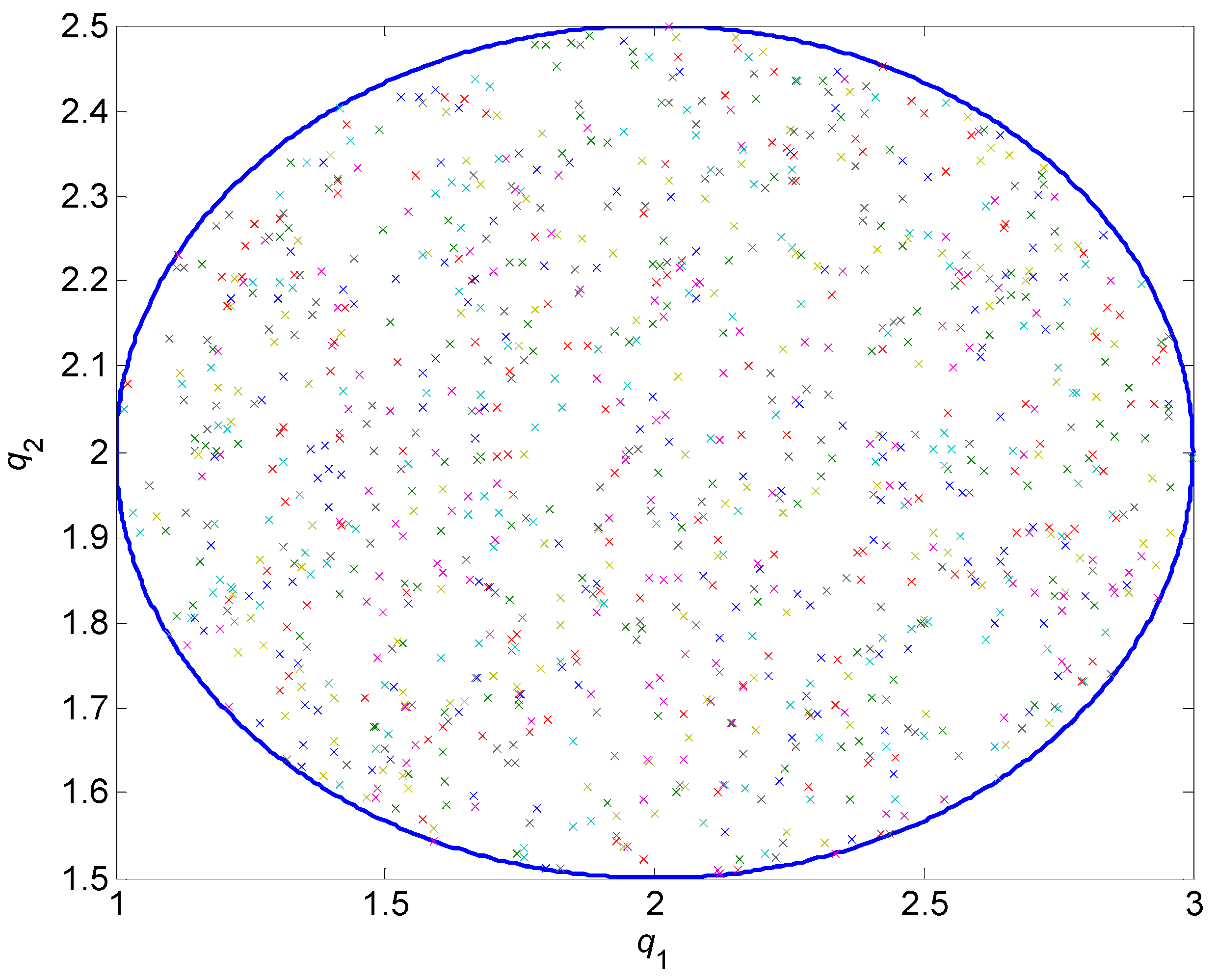
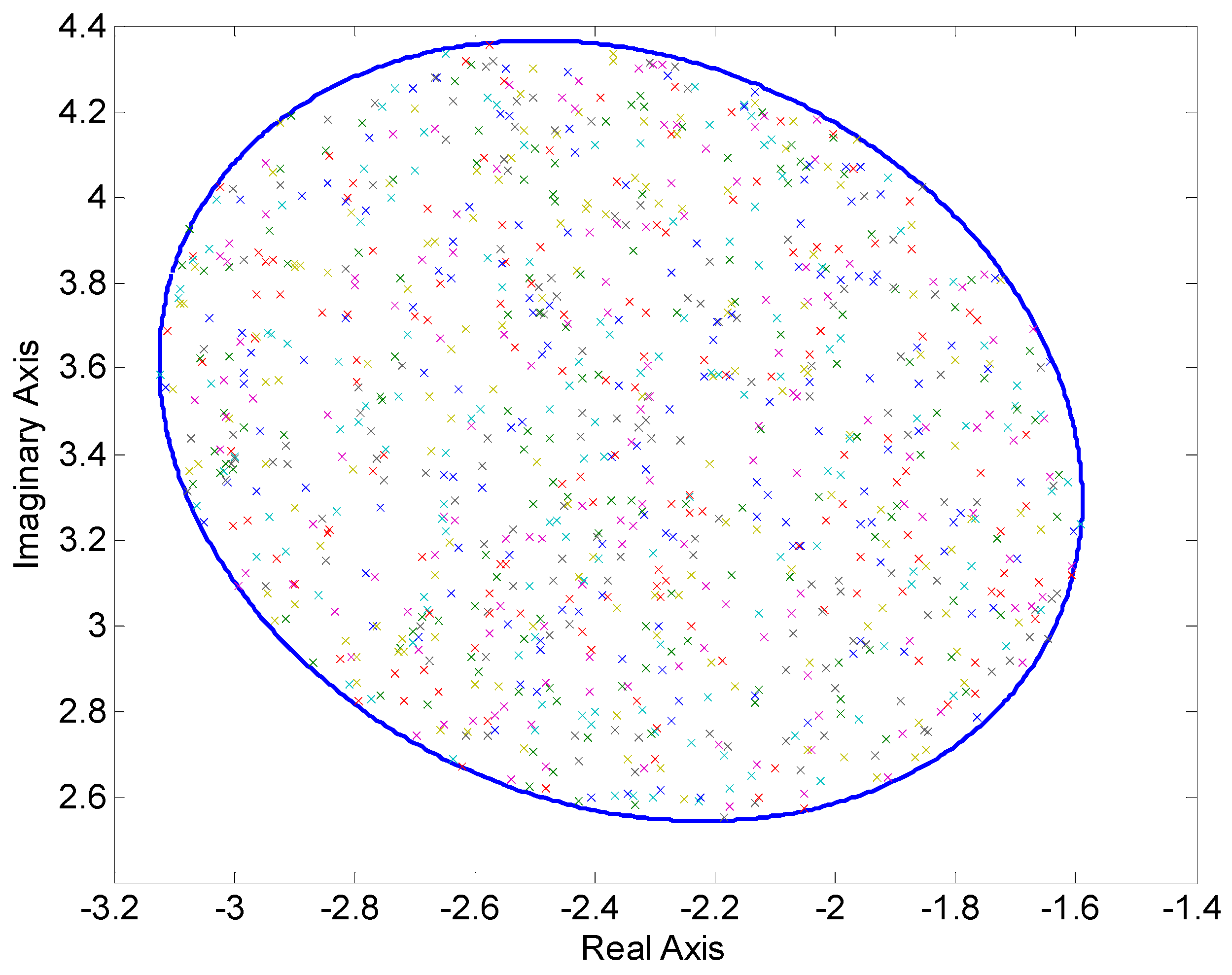
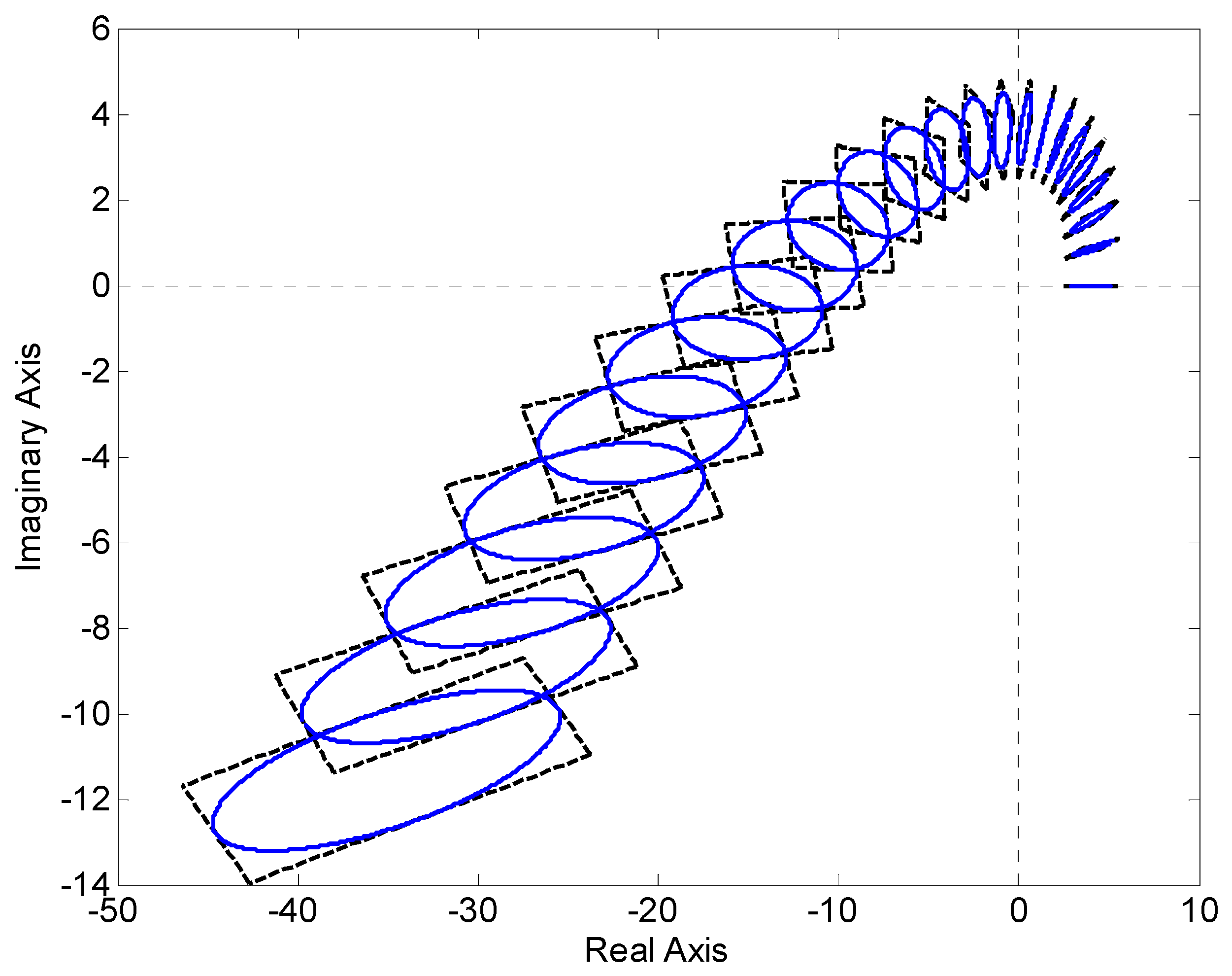
6.1. Example 1—Affine Linear Uncertainty Structure

First, suppose the family of FO polynomials defined by the combination of the uncertain polynomial with affine linear uncertainty structure (inspired by its IO version in [10]):

$$p_{LAF}(s,q)=s^{3.1}+\left(2q_1+q_2+2\right)s^{2.2}+\left(q_1+2q_2+1\right)s^{0.9}+\left(q_1+q_2\right)$$

(19)

and two kinds of uncertainty bounding set:

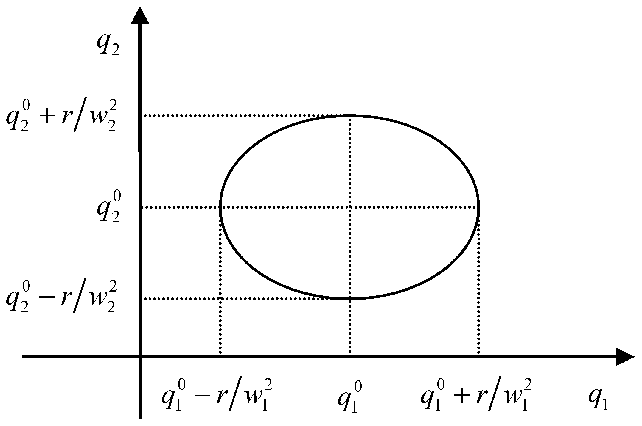
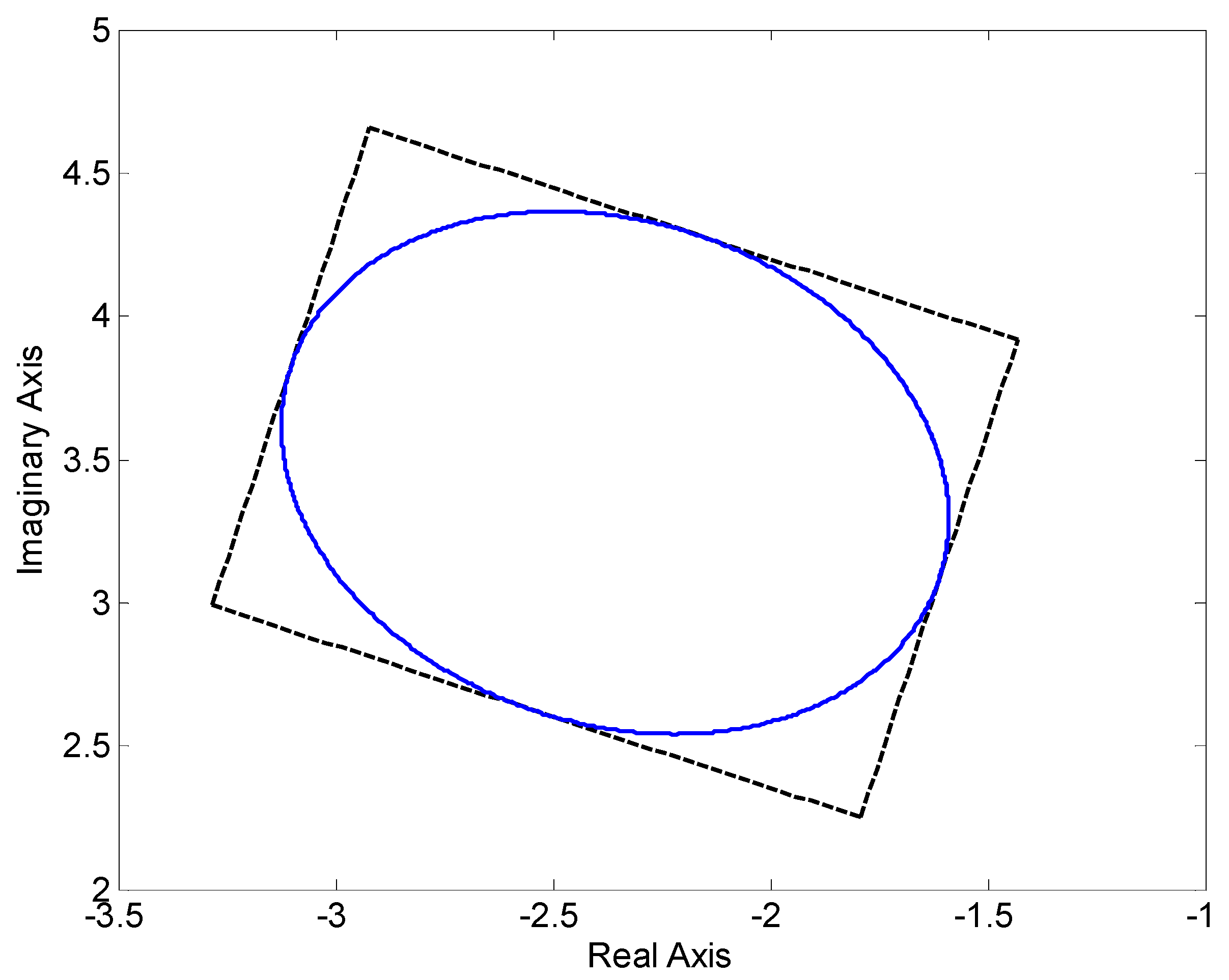
• Weighted L₂ norm (an ellipsoid, or actually an ellipse in this two-dimensional case):

  $$\begin{array}{l}{\Vert q-q^0\Vert }_{2,W}\le 1\\ q^0=\left[2,2\right]\\ W=\left[\begin{array}{cc}{w}_1^2& 0\\ 0& w_2^2\end{array}\right]=\left[\begin{array}{cc}1& 0\\ 0& 2\end{array}\right]\end{array}$$

  (20)

  that is, equivalently:

  $$\begin{array}{l}{\left(q_1-q_1^0\right)}^2+2{\left(q_2-q_2^0\right)}^2\le 1\\ q^0=\left[2,2\right]\end{array}$$

  (21)
• L_∞ norm (a box, or actually a rectangle in this two-dimensional case):

  $$\begin{array}{l}{q}_1\in \left[1,3\right]\\ q_2\in \left[1.5,2.5\right]\end{array}$$

  (22)

The two-dimensional elliptical uncertainty bounding set (20), (21), with two uncertain parameters q₁ and q₂ that may vary within given bounds, is visualized in Figure 2, which shows not only the boundary (blue curve) but also 1000 randomly chosen internal points. Moreover, the rectangle formed by the displayed axes in Figure 2 concurs with the rectangular uncertainty bounding set (22).

The value set of the ellipsoidal family of FO polynomials with affine linear uncertainty structure given by (19) and (20) for the frequency $\omega =1$ is shown in Figure 3. The horizontal axis, labeled as “Real Axis”, represents the real parts of the value set generally defined by (13), and the vertical axis, labeled as “Imaginary Axis” represents the imaginary parts of this value set. The same notation is also used in all the following relevant figures. The plotted value set consists of its boundaries, which are related to the boundaries of the elliptical uncertainty bounding set (20) from Figure 2, and the images of 1000 randomly selected points within this elliptical uncertainty bounding set. As can be seen, all internal points from the parameter space remain inside the value set in the complex plane as well. In other words, the boundaries of the value set are mapped only from the boundaries of the uncertainty bounding set (in the parameter space) for the studied case of the ellipsoidal family of FO polynomials. However, it should be noted that some parts of the boundaries in the uncertain parameter space can generally (in more than two-dimensional case) be mapped into the interior of the value set—see the example at page 142 in [5] where an edge of an uncertain cuboid is mapped to the inside the value set, and see also the Section 6.3 (Example 3). Anyway, it still holds true that the value set boundaries are mapped only from the uncertainty bounding set boundaries. The abovementioned results are valid for the affine linear uncertainty structure (and simpler “independent” one), but they need not be true for more general and more complex uncertainty structures as will be shown later.

Furthermore, Figure 4 compares the value set of the ellipsoidal version of the family (19), (20) (blue solid curve) with the value set of the classical box version of the family (19), (22) (black dashed curve)—both for $\omega =1$. The same comparison but for the value sets in the range of frequencies from 0 to 2.2 with the step 0.1 is shown in Figure 5 (the value sets would reach the fourth quadrant for higher frequencies since the highest order in (19) is 3.1). In compliance with the zero exclusion condition, which is described in the previous Section 5, both ellipsoidal and box version of the family of FO polynomials are robustly stable because all preconditions including the existence of a stable member are fulfilled and the complex plane origin (zero point) is excluded from the plotted value sets.

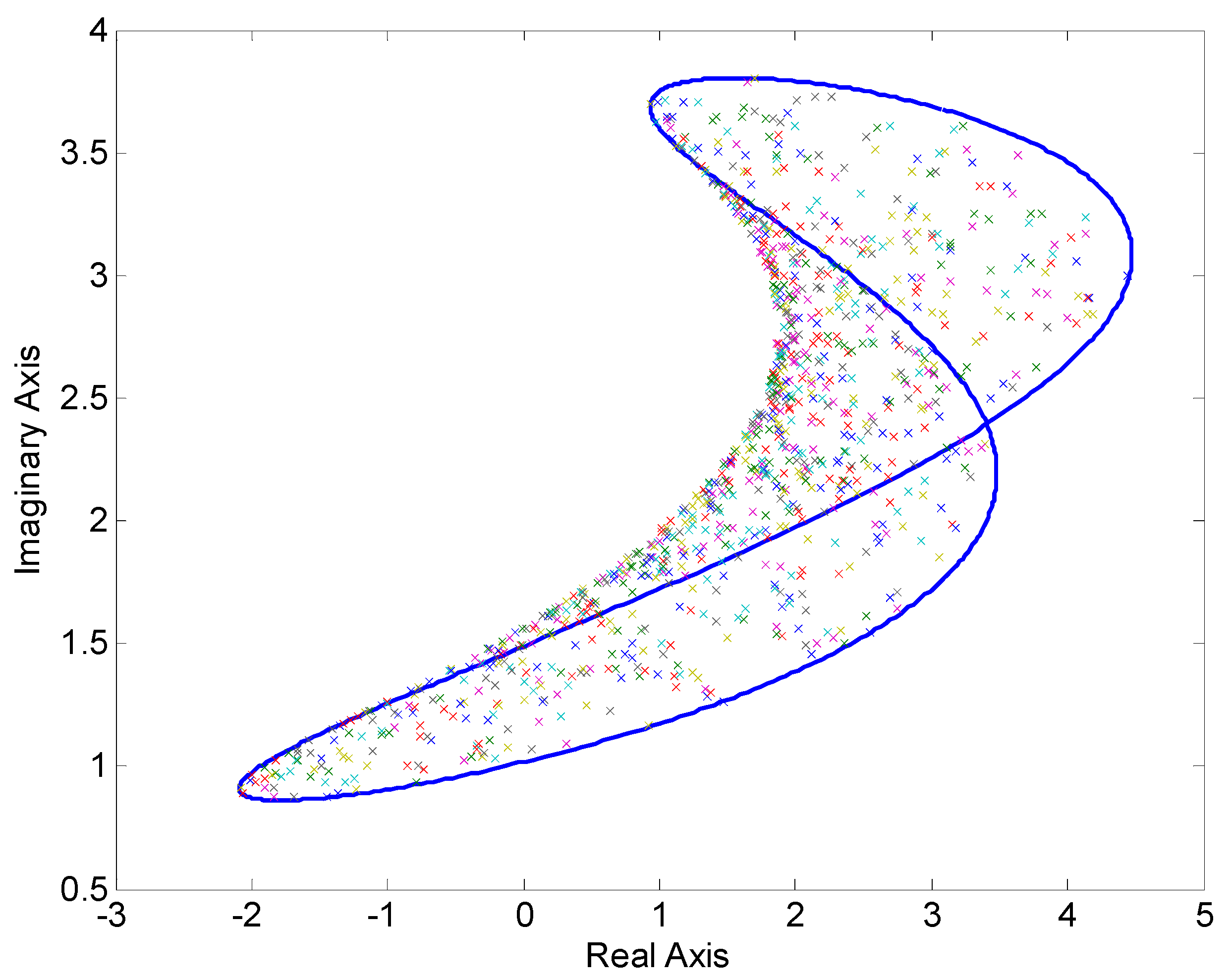
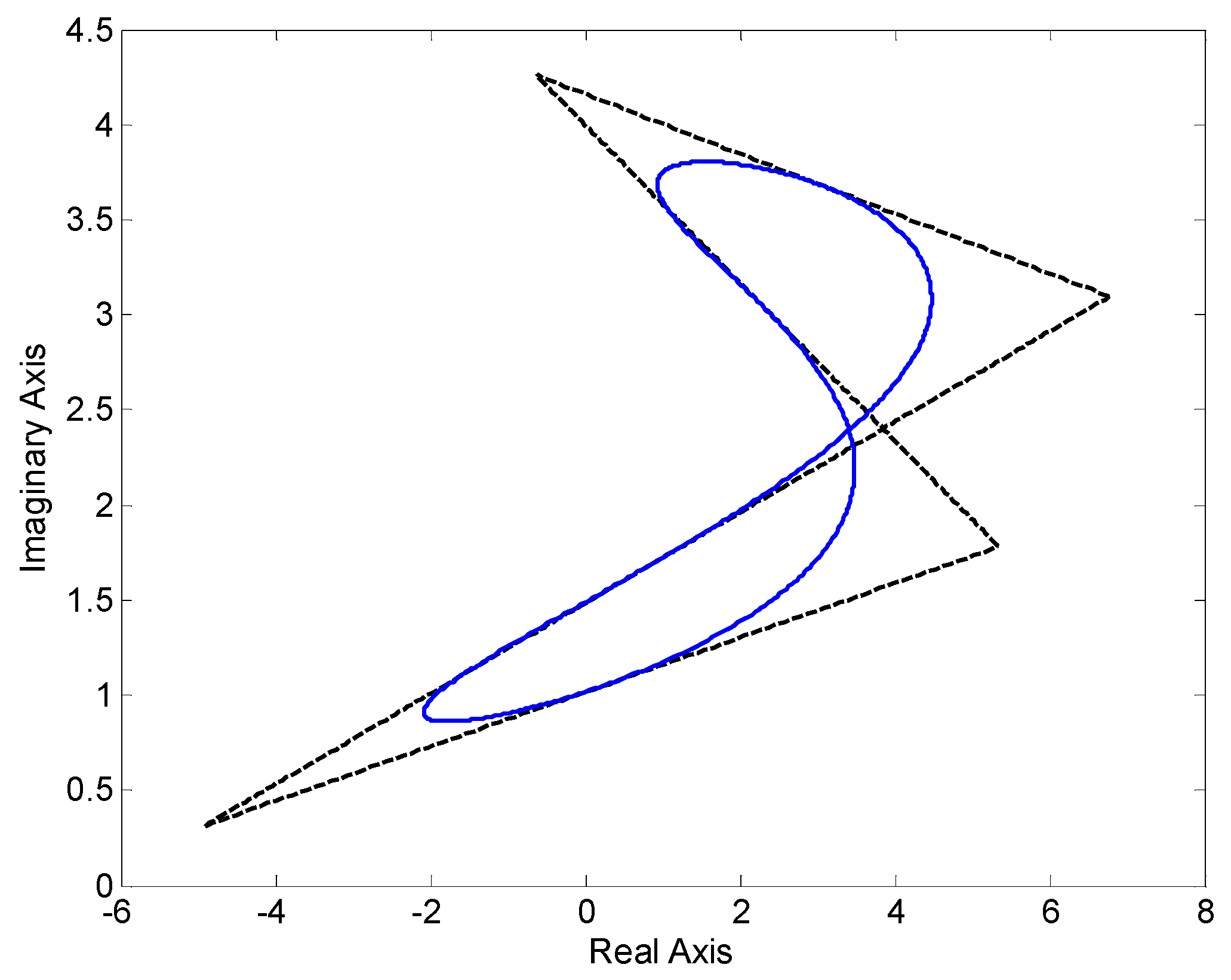
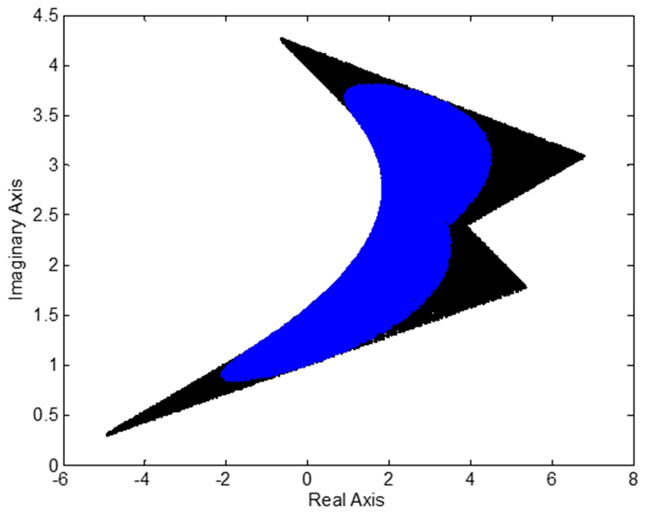
6.2. Example 2—Multilinear Uncertainty Structure

In the second example, assume the family of FO polynomials given by the uncertain polynomial with multilinear uncertainty structure (based on its IO version from [11]):

$$p_{MUL}(s,q)=s^{3.2}+\left(4q_1{q}_2+2\right)s^{2.1}+\left(q_1{q}_2+q_1+q_2+5\right)s^{0.8}+\left(q_1+q_2+3\right)$$

(23)

and, similarly to the Example 1, two types of uncertainty bounding set:

• Weighted L₂ norm:

  $$\begin{array}{l}{\Vert q-q^0\Vert }_{2,W}\le 1\\ q^0=\left[0,0\right]\\ W=\left[\begin{array}{cc}{w}_1^2& 0\\ 0& w_2^2\end{array}\right]=\left[\begin{array}{cc}1& 0\\ 0& 2\end{array}\right]\end{array}$$

  (24)

  i.e.,:

  $$\begin{array}{l}{\left(q_1-q_1^0\right)}^2+2{\left(q_2-q_2^0\right)}^2\le 1\\ q^0=\left[0,0\right]\end{array}$$

  (25)
• L_∞ norm:

  $$\begin{array}{l}{q}_1\in \left[-1,1\right]\\ q_2\in \left[-0.5,0.5\right]\end{array}$$

  (26)

Both elliptical and rectangular uncertainty bounding sets could be visualized easily. The resulting drawing would be almost identical to the Figure 2, except for the range of parameters/axes that would be different.

The value set of the ellipsoidal family of FO polynomials with multilinear uncertainty structure defined by (23) and (24) for the frequency $\omega =1.5$ is shown in Figure 6. Just as in the Example 1, the value set consists of its boundaries connected with the boundaries of the elliptical uncertainty bounding set (24) and the images of 1000 randomly selected points within this uncertainty bounding set. However, unlike the Example 1, not only that the value set is a non-convex shape, but moreover, some internal points from the parameter space create the boundary of the value set in the complex plane. In other words, the boundaries of the value set can be mapped not only from the boundaries in the parameter space but possibly also from the internal points. Obviously, it generally complicates the robust stability analysis of the (FO) polynomial family, because the boundary-guard-based tests are not directly available. Fortunately, the zero exclusion condition is valid.

Comparison of the values set parts that are related to the boundaries in the uncertain parameter space of the ellipsoidal version of the family (23), (24) (blue solid curve) and the box version of the family (23), (26) (black dashed curve) for $\omega =1.5$ is depicted in Figure 7.

Then, the full value sets (including the parts mapped from the internal points in the uncertain parameter space) of the ellipsoidal version of the family (23), (24) (inner blue area) and the box version of the family (23), (26) (outer black area) for $\omega =1.5$ are compared in Figure 8.

The value sets of the ellipsoidal family of FO polynomials with multilinear uncertainty structure (23), (24) for the scale of frequencies from 0 to 3 with step 0.1 is shown in Figure 9. Obviously, the family is robustly unstable because the origin of the complex plane (zero point) is included in the value sets.

6.3. Example 3—Polynomic Uncertainty Structure

In the third example, consider the ellipsoidal family of FO polynomials with polynomic uncertainty structure:

$$\begin{array}{l}{p}_{POL}(s,q)=s^{4.2}+\left(q_1^3+q_2^3+q_3^3+2\right)s^{3.3}+\left(3q_1^5{q}_2^2{q}_3^3+q_1{q}_2{q}_3+5\right)s^{1.8}+\cdots \\ \cdots +\left(q_1^2{q}_2{q}_3^2+q_1{q}_2^2{q}_3+1\right)s^{0.9}+q_1{q}_2{q}_3+1\\ {\Vert q-q^0\Vert }_{2,W}\le 1\\ q^0=\left[0.5,0.5,0.5\right]\\ W=\left[\begin{array}{ccc}{w}_1^2& 0& 0\\ 0& w_2^2& 0\\ 0& 0& w_3^2\end{array}\right]=\left[\begin{array}{ccc}1& 0& 0\\ 0& 2& 0\\ 0& 0& 3\end{array}\right]\end{array}$$

(27)

Note that the uncertainty bounding set is three-dimensional in this event (not just two-dimensional as in the previous two examples). It can be depicted by means of the ellipsoid from Figure 10.

The value sets of the family (27) for the frequencies from 0 to 1.59 with step 0.03 are depicted in Figure 11 (the value sets would reach the fifth quadrant for higher frequencies since the highest order in (27) is 4.2). In this case, it is obtained via gridding the surface area of the ellipsoid from Figure 10 and subsequent calculation of the related value set points. Obviously, the boundary of the uncertainty bounding set is mapped to both the boundary and the interior of the value sets (see the comment in Section 6.1 (Example 1)). According to the zero exclusion condition, the family (27) is robustly stable as it satisfies all preconditions as well as the exclusion of the complex plane origin from the value sets.

6.4. Example 4—General Uncertainty Structure

Finally, assume the ellipsoidal family of FO polynomials with a general uncertainty structure (based on its box version in [9]):

$$\begin{array}{l}{p}_{GEN}(s,q)=s^{3.2}+\left(\cos \left(q_1{q}_2\right)+2\right)s^{2.1}+\left(5\sqrt{\left|q_1\right|}-3\sin \left(q_2\right)-\cos \left(q_1{q}_2\right)+3\right)s^{0.9}+\cdots \\ \cdots +\left(-\sqrt{\left|q_1\right|}+\sin \left(q_2\right)+\cos \left(q_1{q}_2\right)+2\right)\\ {\Vert q-q^0\Vert }_{2,W}\le 1\\ q^0=\left[0,0\right]\\ W=\left[\begin{array}{cc}{w}_1^2& 0\\ 0& w_2^2\end{array}\right]=\left[\begin{array}{cc}1& 0\\ 0& 1\end{array}\right]\end{array}$$

(28)

As can be seen from the Figure 12, which shows the value sets for the frequencies from 0 to 3 with the step 0.1, the family (28) is not robustly stable since the zero exclusion condition is violated.

7. Conclusions

This paper was aimed at the application of the value-set-based graphical technique for analyzing the robust stability of the ellipsoidal families of FO polynomials with complicated parametric uncertainty structure. A set of four extensive illustrative examples was elaborated and discussed in order to demonstrate the applicability of this versatile and effective method to the families of FO polynomials having the ellipsoid-shaped uncertainty bounding set and affine linear, multilinear, polynomic, or general structure of parametric uncertainty. The comparison of the ellipsoidal families with their corresponding box-bounded counterparts was also included.

Since the FO calculus enables considerable improvement in mathematical modeling and (robust) control of dynamical systems compared to the classical IO scenarios, the number of practical applications of FO control systems is expected to increase. Thus, the tools that facilitate the analysis of robust stability for various classes of FO uncertain systems are of growing importance as well. This paper intended to contribute to this mosaic with the application of the value-set-based robust stability investigation method to the ellipsoidal families of FO (characteristic) polynomials with a complicated structure of parametric uncertainty.

The main advantage of the utilized graphical approach is that the robust stability analysis results are obtained with the necessary and sufficient condition by a relatively easy-to-use procedure even for very complicated parametric uncertainty structures. A disadvantage can be seen in the necessity of large computational time for a high number of uncertain parameters or for a dense sampling (gridding) of them.

A potential topic for future research can be seen, among others, in the extension of selected robust stability analysis principles to quantum control systems.

References

1. Simani, S.; Castaldi, P. Robust Control Examples Applied to a Wind Turbine Simulated Model. Appl. Sci. 2018, 8, 29. [Google Scholar] [CrossRef] [Green Version]
2. Sato, T.; Hayashi, I.; Horibe, Y.; Vilanova, R.; Konishi, Y. Optimal Robust PID Control for First- and Second-Order Plus Dead-Time Processes. Appl. Sci. 2019, 9, 1934. [Google Scholar] [CrossRef] [Green Version]
3. Kurokawa, R.; Sato, T.; Vilanova, R.; Konishi, Y. Discrete-Time First-Order Plus Dead-Time Model-Reference Trade-off PID Control Design. Appl. Sci. 2019, 9, 3220. [Google Scholar] [CrossRef] [Green Version]
4. Vasičkaninová, A.; Bakošová, M. Robust Controller Design for a Heat Exchanger Using H2, H, H2/H, and μ-Synthesis Approaches. Acta Chim. Slovaca 2016, 10, 184–193. [Google Scholar] [CrossRef] [Green Version]
5. Barmish, B.R. New Tools for Robustness of Linear Systems; Macmillan: New York, NY, USA, 1994. [Google Scholar]
6. Bhattacharyya, S.P. Robust control under parametric uncertainty: An overview and recent results. Annu. Rev. Control 2017, 44, 45–77. [Google Scholar] [CrossRef]
7. Matušů, R.; Prokop, R. Graphical analysis of robust stability for systems with parametric uncertainty: An overview. Trans. Inst. Meas. Control 2011, 33, 274–290. [Google Scholar] [CrossRef]
8. Matušů, R.; Prokop, R. Robust Stability Analysis for Systems with Real Parametric Uncertainty: Implementation of Graphical Tests in Matlab. Int. J. Circuits Syst. Signal Process. 2013, 7, 26–33. [Google Scholar]
9. Matušů, R.; Şenol, B.; Pekař, L. Robust stability of fractional order polynomials with complicated uncertainty structure. PLoS ONE 2017, 12, e0180274. [Google Scholar] [CrossRef] [Green Version]
10. Matušů, R. Value Sets of Ellipsoidal Polynomial Families with Affine Linear Uncertainty Structure. In Cybernetics and Automation Control Theory Methods in Intelligent Algorithms: Proceedings of the 8th Computer Science On-Line Conference 2019, Volume 3—Advances in Intelligent Systems and Computing (Volume 986); Springer Nature Switzerland AG: Cham, Switzerland, 2019; pp. 255–263. [Google Scholar] [CrossRef]
11. Matušů, R.; Şenol, B. Application of Value Set Concept to Ellipsoidal Polynomial Families with Multilinear Uncertainty Structure. In Computational Statistics and Mathematical Modeling Methods in Intelligent Systems: Proceedings of 3rd Computational Methods in Systems and Software 2019, Volume 2—Advances in Intelligent Systems and Computing (Volume 1047); Springer Nature Switzerland AG: Cham, Switzerland, 2019; pp. 81–89. [Google Scholar] [CrossRef]
12. Hurák, Z.; Šebek, M. New Tools for Spherical Uncertain Systems in Polynomial Toolbox for Matlab. In Proceedings of the Technical Computing Prague 2000, Prague, Czech Republic, 2000; Available online: https://www.humusoft.cz/archive/events/tcp2000/ (accessed on 24 October 2019).
13. Tesi, A.; Vicino, A.; Villoresi, F. Robust Stability of Spherical Plants with Unstructured Uncertainty. In Proceedings of the American Control Conference, Seattle, Washington, WA, USA, 21–23 June 1995. [Google Scholar]
14. Polyak, B.T.; Shcherbakov, P.S. Random Spherical Uncertainty in Estimation and Robustness. In Proceedings of the 39th IEEE Conference on Decision and Control, Sydney, Australia, 12–15 December 2000. [Google Scholar]
15. Matušů, R. Spherical Families of Polynomials: A Graphical Approach to Robust Stability Analysis. Int. J. Circuits Syst. Signal Process. 2016, 10, 326–332. [Google Scholar]
16. Matušů, R. Families of spherical polynomials: Description and robust stability analysis. In Proceedings of the 18th International Conference on Systems, Santorini, Greece, 17–21 July 2014; pp. 606–610. [Google Scholar]
17. Matušů, R.; Prokop, R. Robust Stability Analysis for Families of Spherical Polynomials. In Intelligent Systems in Cybernetics and Automation Theory: Proceedings of the 4th Computer Science On-line Conference 2015 (CSOC2015), Volume 2—Advances in Intelligent Systems and Computing (Volume 348); Springer International Publishing: Cham, Switzerland, 2015; pp. 57–65. [Google Scholar]
18. Kishida, M.; Braatz, R.D. Quality-by-design by skewed spherical structured singular value. IET Control Theory Appl. 2015, 9, 2202–2210. [Google Scholar] [CrossRef] [Green Version]
19. Kishida, M.; Braatz, R.D. Ellipsoidal bounds on state trajectories for discrete-time systems with linear fractional uncertainties. Optim. Eng. 2015, 16, 695–711. [Google Scholar] [CrossRef] [Green Version]
20. Crisalle, O.D.; Ballamundi, R.K. Robust pole-placement technique for plants with ellipsoidally uncertain parameters. Chem. Eng. Sci. 1996, 51, 3193–3202. [Google Scholar] [CrossRef]
21. Raynaud, H.F.; Pronzato, L.; Walter, E. Robust identification and control based on ellipsoidal parametric uncertainty descriptions. Eur. J. Control 2000, 6, 245–255. [Google Scholar] [CrossRef]
22. Barenthin, M.; Hjalmarsson, H. Identification and control: Joint input design and H state feedback with ellipsoidal parametric uncertainty via LMIs. Automatica 2008, 44, 543–551. [Google Scholar] [CrossRef]
23. Henrion, D.; Šebek, M.; Kučera, V. LMIs for robust stabilization of systems with ellipsoidal uncertainty. In Proceedings of the 13th International Conference on Process Control, Štrbské Pleso, Slovakia, 11–14 June 2001. [Google Scholar]
24. Sadeghzadeh, A.; Momeni, H. Fixed-order robust H control and control-oriented uncertainty set shaping for systems with ellipsoidal parametric uncertainty. Int. J. Robust Nonlinear Control 2011, 21, 648–665. [Google Scholar] [CrossRef]
25. Sadeghzadeh, A.; Momeni, H.; Karimi, A. Fixed-order H controller design for systems with ellipsoidal parametric uncertainty. Int. J. Control 2011, 84, 57–65. [Google Scholar] [CrossRef] [Green Version]
26. Sadeghzadeh, A. Identification and robust control for systems with ellipsoidal parametric uncertainty by convex optimization. Asian J. Control 2012, 14, 1251–1261. [Google Scholar] [CrossRef]
27. Sadeghzadeh, A.; Momeni, H. Robust output feedback control for discrete-time systems with ellipsoidal uncertainty. Ima J. Math. Control Inf. 2016, 33, 911–932. [Google Scholar] [CrossRef]
28. Soh, C.B.; Berger, C.S.; Dabke, K.P. On the stability properties of polynomials with perturbed coefficients. IEEE Trans. Autom. Control 1985, 30, 1033–1036. [Google Scholar] [CrossRef]
29. Biernacki, R.M.; Hwang, H.; Bhattacharyya, S.P. Robust stability with structured real parameter perturbations. IEEE Trans. Autom. Control 1987, 32, 495–506. [Google Scholar] [CrossRef]
30. Barmish, B.R.; Tempo, R. On the spectral set for a family of polynomials. IEEE Trans. Autom. Control 1991, 36, 111–115. [Google Scholar] [CrossRef]
31. Tsypkin, Y.Z.; Polyak, B.T. Frequency domain criteria for lp-robust stability of continuous linear systems. IEEE Trans. Autom. Control 1991, 36, 1464–1469. [Google Scholar] [CrossRef]
32. Matušů, R.; Pekař, L. Robust Stability of Thermal Control Systems with Uncertain Parameters: The Graphical Analysis Examples. Appl. Therm. Eng. 2017, 125, 1157–1163. [Google Scholar] [CrossRef]
33. Tan, N.; Özgüven, Ö.F.; Özyetkin, M.M. Robust stability analysis of fractional order interval polynomials. ISA Trans. 2009, 48, 166–172. [Google Scholar] [CrossRef] [PubMed]
34. Şenol, B.; Yeroğlu, C. Computation of the Value Set of Fractional Order Uncertain Polynomials: A 2q Convex Parpolygonal Approach. In Proceedings of the 2012 IEEE International Conference on Control Applications, Dubrovnik, Croatia, 3–5 October 2012. [Google Scholar]
35. Şenol, B.; Yeroğlu, C. Robust Stability Analysis of Fractional Order Uncertain Polynomials. In Proceedings of the 5th IFAC Workshop on Fractional Differentiation and its Applications, Nanjing, China, 14–17 May 2012. [Google Scholar]
36. Yeroğlu, C.; Şenol, B. Investigation of robust stability of fractional order multilinear affine systems: 2q-convex parpolygon approach. Syst. Control Lett. 2013, 62, 845–855. [Google Scholar] [CrossRef]
37. Oldham, K.B.; Spanier, J. Fractional Calculus: Theory and Applications of Differentiation and Integration to Arbitrary Order; Academic Press: New York, NY, USA; London, UK, 1974. [Google Scholar]
38. Podlubný, I. Fractional Differential Equations; Academic Press: San Diego, CA, USA, 1999. [Google Scholar]
39. Machado, J.A.T.; Kiryakova, V.; Mainardi, F. Recent history of fractional calculus. Commun. Nonlinear Sci. Numer. Simul. 2011, 16, 1140–1153. [Google Scholar] [CrossRef] [Green Version]
40. Gutiérrez, R.E.; Rosário, J.M.; Machado, J.A.T. Fractional Order Calculus: Basic Concepts and Engineering Applications. Math. Probl. Eng. 2010, 2010. [Google Scholar] [CrossRef]
41. Axtell, M.; Bise, M.E. Fractional calculus applications in control systems. In Proceedings of the 1990 National Aerospace and Electronics Conference, Dayton, OH, USA, 21–25 May 1990. [Google Scholar]
42. Podlubný, I. Fractional-Order Systems and PIλDμ-Controllers. IEEE Trans. Autom. Control 1999, 44, 208–214. [Google Scholar] [CrossRef]
43. Chen, Y.; Petráš, I.; Xue, D. Fractional Order Control—A Tutorial. In Proceedings of the 2009 American Control Conference, St. Louis, MO, USA, 10–12 June 2009. [Google Scholar]
44. Petráš, I. Stability of fractional-order systems with rational orders: A survey. Fract. Calc. Appl. Anal. 2009, 12, 269–298. [Google Scholar]
45. Xue, D. Fractional-Order Control Systems: Fundamentals and Numerical Implementations; De Gruyter: Berlin, Germany, 2017. [Google Scholar]
46. Altafini, C.; Ticozzi, F. Modeling and Control of Quantum Systems: An Introduction. IEEE Trans. Autom. Control 2012, 57, 1898–1917. [Google Scholar] [CrossRef]
47. Dong, D.; Petersen, I.R. Quantum control theory and applications: A survey. IET Control Theory Appl. 2010, 4, 2651–2671. [Google Scholar] [CrossRef] [Green Version]
48. Chen, C.; Wang, L.-C.; Wang, Y. Closed-Loop and Robust Control of Quantum Systems. Sci. World J. 2013, 2013. [Google Scholar] [CrossRef] [PubMed]
49. Petersen, I.R.; Ugrinovskii, V.; James, M.R. Robust stability of uncertain linear quantum systems. Philos. Trans. R. Soc. A Math. Phys. Eng. Sci. 2012, 370, 5354–5363. [Google Scholar] [CrossRef] [PubMed] [Green Version]
50. Matušů, R.; Şenol, B.; Vašek, V. Robust Stability of Fractional-Order LTI Systems with Independent Structure of Ellipsoidal Parametric Uncertainty. In Proceedings of the 30th DAAAM International Symposium, Zadar, Croatia, 23–26 October 2019. [Google Scholar]
51. Lu, J.-G.; Chen, Y. Stability and stabilization of fractional-order linear systems with convex polytopic uncertainties. Fract. Calc. Appl. Anal. 2013, 16, 142–157. [Google Scholar] [CrossRef]
52. Šebek, M. Robustní řízení (Robust Control); PDF slides for the course on Robust Control; Czech Technical University in Prague: Prague, Czech Republic, 2002. [Google Scholar]
53. Matušů, R.; Prokop, R. Robust Stability of Fractional Order Time-Delay Control Systems: A Graphical Approach. Math. Probl. Eng. 2015, 2015. [Google Scholar] [CrossRef] [Green Version]
54. Tempo, R.; Calafiore, G.; Dabbene, F. Randomized Algorithms for Analysis and Control of Uncertain Systems: With Applications; Springer: London, UK, 2013. [Google Scholar]
55. Barmish, B.R.; Lagoa, C.M. The uniform distribution: A rigorous justification for its use in robustness analysis. Math. ControlSignalsSyst. 1997, 10, 203–222. [Google Scholar] [CrossRef]
Figure 1. Ellipsoidal geometry defined by weighted Euclidean norm [5,15].
Applsci 09 05451 g001
Figure 2. Elliptical uncertainty bounding set (20) with 1000 randomly chosen internal points.
Applsci 09 05451 g002
Figure 3. The value set of the family (19), (20) for ω = 1 with the images of 1000 randomly chosen internal points from the elliptical uncertainty bounding set (Figure 2).
Applsci 09 05451 g003
Figure 4. Comparison of the value sets of the family (19), (20) (blue solid curve) and of the family (19), (22) (black dashed curve) for ω = 1 .
Applsci 09 05451 g004
Figure 5. Comparison of the value sets of the family (19), (20) (blue solid curves) and of the family (19), (22) (black dashed curves) for ω = 0 : 0.1 : 2.2 .
Applsci 09 05451 g005
Figure 6. The value set of the family (23), (24) for ω = 1.5 with the images of 1000 randomly chosen internal points from the elliptical uncertainty bounding set.
Applsci 09 05451 g006
Figure 7. Comparison of the value set parts that are related to the boundaries in the uncertain parameter space for the family (23), (24) (blue solid curve) and the family (23), (26) (black dashed curve) for ω = 1.5 .
Applsci 09 05451 g007
Figure 8. Comparison of the complete values sets of the family (23), (24) (inner blue area) and the family (23), (26) (outer black area) for ω = 1.5 .
Applsci 09 05451 g008
Figure 9. The value sets of the family (23), (24) for ω = 0 : 0.1 : 3 .
Applsci 09 05451 g009
Figure 10. Ellipsoidal uncertainty bounding set for the family (27).
Applsci 09 05451 g010
Figure 11. The value sets of the family (27) for ω = 0 : 0.02 : 1.59 .
Applsci 09 05451 g011
Figure 12. The value sets of the family (28) for ω = 0 : 0.1 : 3 .
Applsci 09 05451 g012