Article

Receptance-Based Dominant Eigenvalues Computation of Controlled Vibrating Systems with Multiple Time-Delays Using a Contour Integral Method

1
School of Mechanical Engineering, Wuhan Polytechnic University, Wuhan 430023, China
2
School of Engineering, University of Liverpool, The Quadrangle, Liverpool L693GH, UK
3
Hubei Provincial Engineering Technology Research Center of Fish Processing Equipment, Wuhan 430023, China
*
Author to whom correspondence should be addressed.
Appl. Sci. 2019, 9(23), 5263; https://doi.org/10.3390/app9235263
Submission received: 26 October 2019 / Revised: 15 November 2019 / Accepted: 29 November 2019 / Published: 3 December 2019
(This article belongs to the Section Acoustics and Vibrations)

Abstract

:
The computation of dominant eigenvalues of second-order linear control systems with multiple time-delays is tackled by using a contour integral method. The proposed approach depends on a reduced characteristic function and the associated characteristic matrix comprised of measured open-loop receptances. This reduced characteristic function is derived from the original characteristic function of the second-order time delayed systems based on the reasonable assumption that eigenvalues of the closed-loop system are distinct from those of the open-loop system, and has the same eigenvalues as those of the original. Then, the eigenvalues computation is equivalent to solve a nonlinear eigenvalue problem of the associated characteristic matrix by using a contour integral method. The proposed approach also utilizes the spectrum distribution features of the retarded time-delay systems. Finally, numerical examples are given to illustrate the effectiveness of the proposed approach.

1. Introduction

Many mechanical and structural systems under active vibration control can be described as linear time-delayed systems (TDSs) due to sensing and actuation delays. The distribution of the eigenvalues (also known as poles or characteristic roots) of such a system on the complex plane determines the stability and dynamic behaviour of the systems. However, the characteristic equation of a TDS contains an infinite number of roots (i.e., eigenvalues) due to its transcendental nature, it is impossible and unnecessary to determine all its roots. For a TDS of retarded type (which makes up the majority of vibration suppression problems of closed-loop control systems), the overall dynamics is mainly dominated by those eigenvalues that lie closely to the imaginary axis, namely, the dominant eigenvalues.
There are some ways to numerically determine a part of eigenvalues within a specified region in the complex plane for a retarded or neutral TDS with constant delays [1]. In addition to traditional methods for computing the zeros of analytic functions, e.g., the well-known Newton’s method and recently proposed QPmR algorithm [2], two other groups of methods are usually found in the literature. In addition, the Lambert W function can also be used, e.g., [3]. The first group of methods are based on an approximation of the solution map using linear multi-step methods [4,5] or Runge–Kutta methods [6]. The second group of methods are based on a discretization of the partial differential equation representation of a TDS, using, e.g., Runge–Kutta methods [7], spectral methods [8], or pseudospectral methods [9]. In both groups of methods, the required eigenvalues of a TDS are determined via the eigenvalues of a matrix resulting from the approximation. It is well known that the aforementioned methods are fast and numerically reliable, and they all depend upon the usage of mathematical models, e.g., delay differential equations, of the system. Thus, it is a prerequisite to require the exact knowledge of system matrices such as, for example, mass, damping and stiffness matrices of the system discussed in this paper, which undoubtedly involves errors in relation to practical systems and quite often are not available.
For mechanical and structural systems whose equations of motion are naturally formulated in the second-order setting, the second-order time delayed systems are generally analysed in the first-order state-space framework after a transformation. Another interesting and useful scheme still in development is to use nonparametric models, e.g., measured receptances, which was originally developed to design linear vibration control of the systems without delay and required knowledge of the system matrices [10,11,12]. There were some works on full/partial eigenvalue assignment of second-order time delayed systems using the receptance method [13,14,15,16,17]. Additionally, a simple stability criterion for second-order systems with time-varying delay based on the receptance approach was presented in [18]. When computing the eigenvalues of these multidimensional systems with constant time delay and conducting a posteriori stability analysis, however, these literatures [13,14,15,16,17] also adopted the aforementioned methods that require the availability of the system matrices. Recently, some authors of this paper proposed a reduced characteristic function derived from the original characteristic function of the second-order time delayed systems. This characteristic function is comprised of “measured” open-loop receptances without requiring the knowledge of system matrices. A Newton-type method was adopted to compute the dominant eigenvalues of the system via this characteristic function [19].
This paper addresses the computation of dominant eigenvalues for second-order systems with multiple constant time-delays using a contour integral method. For completeness of description the reduced characteristic function f m ( λ ) and the associated characteristic matrix J m ( λ ) of the closed-loop system are firstly derived. They have the same eigenvalues (or characteristic roots) as those of the closed-loop system and involve only control gains, time-delay parameters, and the measured open-loop receptances at the sensor/actuator coordinates. Then, one of the methods that are used to solve nonlinear eigenvalue problems, a contour integral method, is adopted to determine the required eigenvalues from the characteristic matrix J m ( λ ) . The proposed approach does not require the knowledge of system matrices and works on J m ( λ ) with a significantly smaller size than that of the original system. Especially, it does not need to provide initial approximations of calculated eigenvalues, which is the major difference between the proposed approach and that in [19].
The paper is organized as follows. In Section 2, the system involved is described, and the reduced characteristic function f m ( λ ) and the associated characteristic matrix J m ( λ ) are derived. A contour integral method is briefly reviewed and the computational procedure of the dominant eigenvalues are presented in Section 3. In Section 4, a numerical example is provided to demonstrate the proposed approach. Conclusions are finally drawn in Section 5.

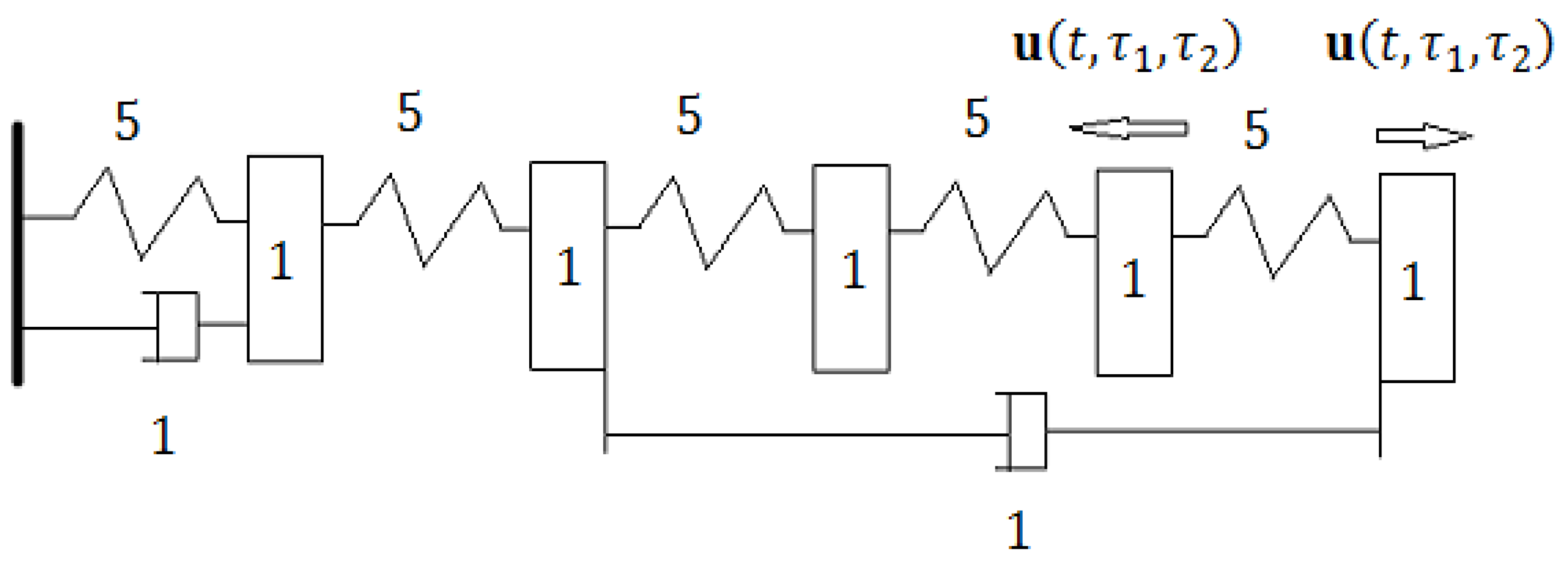
2. System Description and Reduced Characteristic Function

A linear second-order controlled system with time-delay is described by:
M x ¨ ( t ) + C x ˙ ( t ) + K x ( t ) = B u ( t , τ 1 , τ 2 ) + f ( t )
u ( t , τ 1 , τ 2 ) = G 1 x ( t τ 1 ) G 2 x ˙ ( t τ 2 )
where M , C , and K are known as the n × n mass, damping, and stiffness matrices, respectively; u is a control force vector and f is an external applied force vector; B is the n × p control input distribution matrix; G 2 and G 1 are the p × n velocity and displacement feedback gain matrices respectively, and p < n; τ 1 and τ 2 are the displacement and velocity feedback time-delays, respectively. Substituting (2) into (1) gives
M x ¨ ( t ) + C x ˙ ( t ) + K x ( t ) = B ( G 1 x ( t τ 1 ) G 2 x ˙ ( t τ 2 ) ) + f ( t )
Laplace transform of (3) gives
( s 2 M + s C + K ) x ( s ) = B ( G 1 e s τ 1 + s G 2 e s τ 2 ) x ( s ) + f ( s )
[ s 2 M + s C + K + B ( G 1 e s τ 1 + s G 2 e s τ 2 ) ] x ( s ) = f ( s )
Then, the full n × n receptance matrices of the open-loop and closed-loop systems are represented by
H 0 ( s ) = ( s 2 M + s C + K ) 1
H c ( s ) = [ H 0 1 ( s ) + B ( G 1 e s τ 1 + s G 2 e s τ 2 ) ] 1
The closed-loop receptance matrix H c ( s ) for the system with delay can be directly related to the open-loop receptance matrix H 0 ( s ) by using the Sherman–Morrison–Woodbury formula as follows:
H c ( s ) = H 0 ( s ) H 0 ( s )   B [ I p + ( G 1 e s τ 1 + s G 2 e s τ 2 ) H 0 ( s )   B ] 1 ( G 1 e s τ 1 + s G 2 e s τ 2 ) H 0 ( s )
The characteristic function of the second-order linear time-delay system (5) is given in the form
f ( λ ) = det ( Z ( λ ) ) = det [ λ 2 M + λ C + K + B ( G 1 e λ τ 1 + λ G 2 e λ τ 2 ) ]
where Z ( λ ) = λ 2 M + λ C + K + B ( G 1 e λ τ 1 + λ G 2 e λ τ 2 ) is the so-called dynamic stiffness matrix of the closed-loop system (5), and Z ( λ ) = H c 1 ( λ ) from (7). f ( λ ) is a transcendental function containing some exponential terms, also called quasi-polynomial, which has an infinite number of roots. The roots of f ( λ ) are also known as eigenvalues (poles or characteristic roots) of (5), whose distribution on the complex plane determines the stability and dynamic behaviour of (5).
Now the reduced form of characteristic function (9) and the corresponding characteristic equation are presented. Without loss of generality, assume that the eigenvalues of the closed-loop system with delay are distinct from those of the open-loop system. Suppose that A and Q are nonsingular matrices of appropriate orders. Based on the following determinant formula given as,
| A + E Q F | = | A | | Q | | Q 1 + F A 1 E |
then, f ( λ ) in (9) can be rewritten as follows:
f ( λ ) = det [ λ 2 M + λ C + K ] det [ I p + ( G 1 e λ τ 1 + λ G 2 e λ τ 2 ) H 0 m ( λ ) ]
with H 0 m ( s ) = H 0 ( s ) B , which is the n × p open-loop receptance matrix. Formula (11) holds for any λ except for finite eigenvalues λ 0 i   (i = 1, 2, …, 2n) of the open-loop system. Then, the characteristic roots of (11), i.e., eigenvalues of the closed-loop system (5), satisfy the following reduced characteristic equation
f m ( λ ) = det [ I p + ( G 1 e λ τ 1 + λ G 2 e λ τ 2 ) H 0 m ( λ ) ] = 0
with the following p × p reduced characteristic matrix
J m ( λ ) = I p + ( G 1 e λ τ 1 + λ G 2 e λ τ 2 ) H 0 m ( λ )
Solving eigenvalues of (5) now become finding roots of f m ( λ ) in the complex plane, and this can also be considered a nonlinear eigenvalue problem (NEP) of matrix-valued function J m ( λ ) which depends nonlinearly on a single scalar parameter λ . Either of them is a non-trivial task. In what follows, a contour integration method used to solve the present nonlinear eigenvalue problem is introduced, which is intended to tackle the problem via J m ( λ ) .

3. The Contour Integral Method for Solving NEP

3.1. A Contour Integral Method

In this paper, a typical NEP under consideration is as follows. Given a (bounded) domain Ω ⊂ ℂ and a matrix-valued function T :   Ω p × p analytic in Ω, one wants to compute the values λ Ω (eigenvalues) and v p , v 0 (eigenvectors) such that
T ( λ ) v = 0
A class of numerical methods for NEPs has recently been developed based on contour integration [20,21,22,23,24]. These methods solve NEPs using the Smith form and Keldysh’s theorem for the analytic matrix-valued function, respectively. One of the latter, Beyn’s algorithm [22], is used as a basis for introducing the method. For notational simplicity when explaining the algorithm, it is assumed that the eigenvalues in which one is interested are simple. As for the more general case, the interested reader is referred to [22]. Additionally, throughout this paper the superscripts H and −1 for a matrix represent the conjugate transpose and the inverse operation, respectively.
Beyn’s algorithm is based on Keldysh’s theorem as follows:
Theorem 1.
(Keldysh’ s theorem [22,24]). Let Φ Ω be a compact subset. Let λ k for k = 1, …, m denote the eigenvalues of T ( λ ) in Φ . Let v k and w k for k = 1, …, m denote their left and right eigenvectors, such that
T ( λ k ) v k = 0 ,   w k H T ( λ k ) = 0 ,   w k H T ( λ k ) v k = 1 .
Then, there is a neighbourhood Π of Φ in Ω and an analytic matrix-valued function L: Π p × p such that the resolvent T 1 ( z ) can be written as
T 1 ( z ) = k = 1 m v k w k H ( z λ k ) 1 + L ( z )
for all z Π \ { λ 1 ,   , λ m } .
The core idea of Beyn’s method is to use formula (16) for the resolvent, and derive the following expression for the corresponding contour integral by utilizing the classical residue theorem.
Lemma 1
[22]. Suppose that T ( z ) has no eigenvalues on a closed contour C Ω and has finitely many eigenvalues { λ 1 , , λ m } lying inside this contour, then, for any function φ ( z ) :   Ω that is analytic in Ω ,
( 2 π i ) 1 C φ ( z ) T 1 ( z ) d z = k = 1 m φ ( z ) v k w k H = V φ ( Λ ) W H
where the columns of V , W p × m are the right and left eigenvectors, respectively, normalized as in (15), and Λ m × m is the diagonal matrix of the eigenvalues.
For the problem discussed in this paper, the number m of eigenvalues { λ 1 ,   , λ m } lying inside C is usually larger than the size p of T ( z ) . In this case, one needs to use higher-order moments in (17), that is, employ different choices of function φ ( z ) , e.g., the monomials φ ( z ) = z 0 , z 1 , z 2 , etc. Now, one multiplies (17) from the right by a constant random probing matrix R p × p . For any k = 0, 1, …, q ( q > 0 is a given as an integer), one defines
A k = ( 2 π i ) 1 C   z k T 1 ( z ) R d z = V Λ k W H R
and arrange these matrices in q p × q p block-Hankel matrices as follows:
B 0 = [ A 0 A q 1 A q 1 A 2 q 2 ]   and   B 1 = [ A 1 A q A q A 2 q 1 ]
Further, defining the following matrices
V q = [ V V Λ q 1 ]   q p × m   and   W q H = [ W H R , , Λ q 1 W H R ] m × q p
Then, one has factorizations for B 0 and B 1 by (18)
B 0 = V q W q H   and   B 1 = V q Λ W q H
Here, one needs an assumption which is fulfilled in the generic case (e.g., q m ), that is,
rank ( V q ) = rank ( W q H ) = m
Now the next step is to compute an economy-size singular value decomposition (SVD) of B 0
B 0 = V q W q H = V 0 Σ 0 W 0 H ,   V 0 q p × m ,   W 0 q p × m ,   Σ 0 = diag ( σ 1 , , σ m )
Since range ( V q ) = range ( V 0 ) , there exists an invertible matrix X m × m such that V q = V 0 X . Substituting the expression V q into V q W q H = V 0 Σ 0 W 0 H of (23) yields
W q H = X 1 Σ 0 W 0 H
This relation can be used to remove W q H from B 1 = V q Λ W q H , i.e.,
B 1 = V 0 X Λ X 1 Σ 0 W 0 H
Until now, one has thus arrived at
P = V 0 H B 1 W 0 Σ 0 1 = X Λ X 1
showing that the eigenvalue decomposition of the computable matrix P leads to matrices Λ and X . To summarize, the solution of the nonlinear eigenvalue problem (14) inside the given contour C can be reduced to the solution of the linear eigenvalue problem (26), hence the eigenvalues of the NEP can be obtained from the eigenvalues of P , and the corresponding right eigenvectors can be retrieved from the columns of V q = V 0 X . A similar approach was proposed by Asakura et al. [21] using the Smith normal form to express T 1 ( z ) .

3.2. Practical Applications

In what follows, some discussions about the contour integral method are presented from the perspective of practical applications, which involve the numerical implementation of the method itself and computation of dominant eigenvalues of controlled structures with multiple time-delays.
First, one typically does not know a priori number m of the simple eigenvalues inside the prescribed contour C . However, as long as the order number q of moments in (18) is chosen large enough, such that Σ 0 of the SVD of B 0 in (23) contains at least one zero singular value. One can detect m by the rank test of the matrix B 0 , for example, by counting the number of singular values of B 0 that are above a user-defined tolerance, and obtain a truncated SVD of B 0 with rank m as in (23). Alternatively, counting the eigenvalues can also be achieved by the argument principle,
( 2 π i ) 1 C g ( z ) g ( z ) d z = N z N p
where g ( z ) = det ( T ( z ) ) , N z and N p denote the number of roots (i.e., eigenvalues of T ( z ) ) and poles of g ( z ) within the contour C in the complex plane, respectively. By using the following trace relation
g ( z ) g ( z ) = trace ( T 1 ( z ) T ( z ) )
The expression (27) can be rewritten as
( 2 π i ) 1 C trace ( T 1 ( z ) T ( z ) ) d z = N z N p
Ordinarily, requiring prior knowledge of N p in (27) or (29) hinders one from determining N z . Fortunately, for controlled systems involved in this paper the number N p of all poles of its reduced characteristic function f m ( z ) = det ( J m ( z ) ) inside a given contour C is identical to that of all poles of its open-loop receptances H 0 m ( λ ) in (12) or (13) within the same contour (based on the assumption that these poles are simple), and the latter can be determined experimentally.
Second, the numerical evaluation of the contour integrals for A k in (18) is usually performed by the trapezoid sum for which nc quadrature points are used. It is preferred to choose the contour C to be a circle with C = α + β e i θ , where α and β are the center and radius of C , respectively, because the quadrature error in this case yields the exponential decay with an exponent that depends on the product of the number of quadrature nodes and the smallest distance of the eigenvalues to the contour [22]. To improve numerical conditioning, one also needs to shift and scale the weight function zk in (18). Thus, a discretized version of (18) is obtained,
A k 1 n c j = 0 n c 1 ( ω j α β ) k + 1 T 1 ( ω j ) R ,   k = 0 , 1 , , 2 q 1 .
where ω j = α + β e 2 π i ( j + 1 / 2 ) / n c for j = 0, 1, …, nc−1. Additionally, the integrand T 1 ( ω j ) R is the solution Y ( ω j ) of the linear system
T ( ω j ) Y ( ω j ) = R
evaluated at each quadrature point ω j .
Third, the second-order time delayed systems discussed in this paper are TDSs of retarded type. Their eigenvalues distribution has some ‘nice’ features [25,26], for example, there are only a finite number of eigenvalues in any given right half complex plane, the eigenvalues with high frequencies tend to be far off the imaginary axis in the left half complex plane and the dominant eigenvalues (i.e., the rightmost eigenvalues in some sense) have the small modulus and low frequencies. These interesting properties will have consequences on the computation of dominant eigenvalues and a choice of the size of C .Thus, it is the suitable choice for C to be a closed circle centered at the origin with a proper radius R in the complex plane. Obviously, the correct determination of radius R of C is a crucial factor for the computation of dominant eigenvalues. As a rule of thumb, radius R can be chosen to be slightly larger than the largest modulus among dominant eigenvalues of the closed-loop system without time-delays (i.e., τ 1 = τ 2 = 0 ) . These eigenvalues could be approximated by solving a NEP of the following matrix from J m ( λ ) via the contour integral method,
J m 1 ( λ ) = I p + ( G 1 + λ G 2 ) H 0 m ( λ ) .

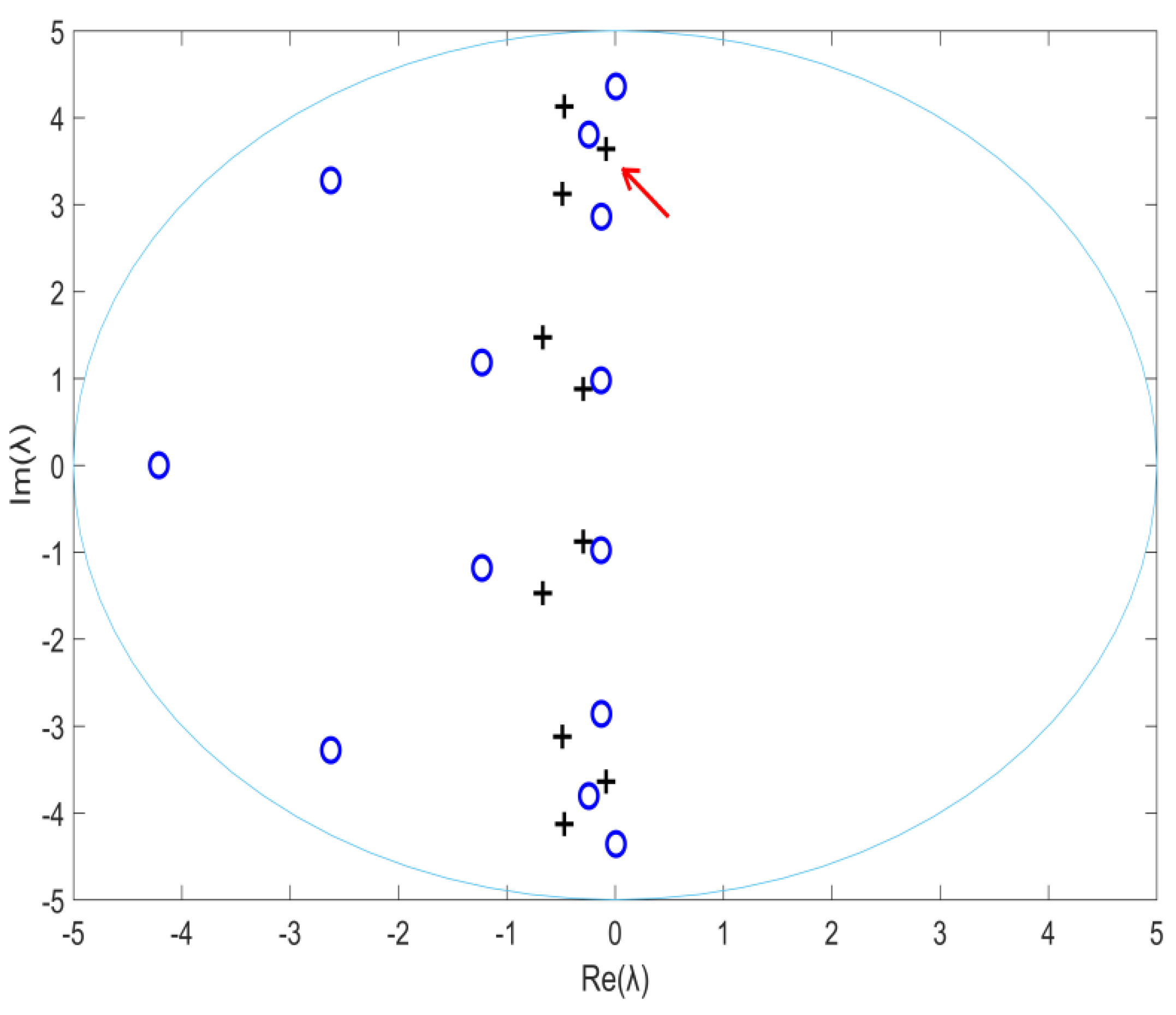
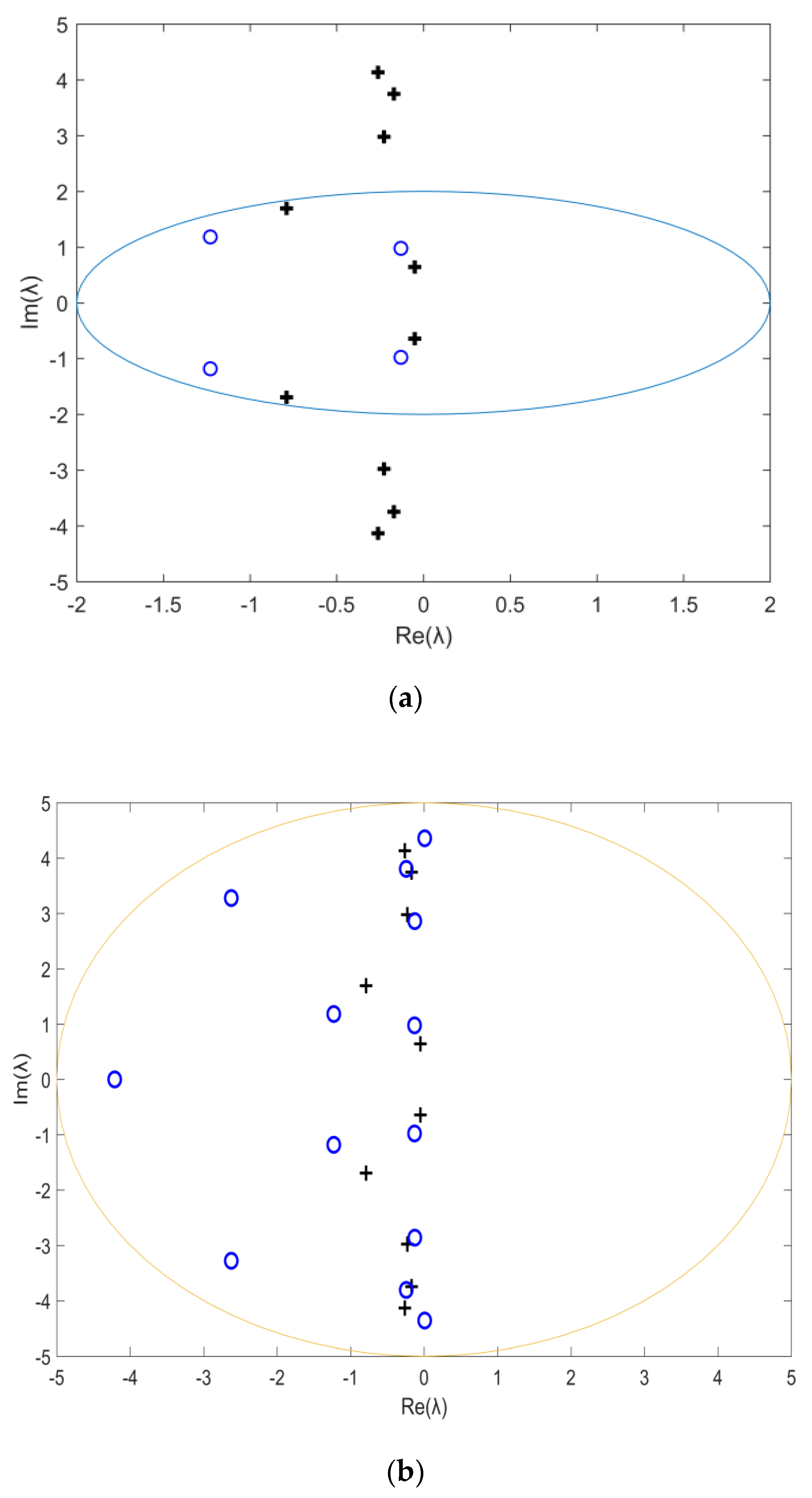
4. Numerical Examples

Consider a five-degree of freedom system, as shown in Figure 1, with the following system matrices [27],
M = I , C = [ 1 0 0 0 0 0 1 0 0 1 0 0 0 0 0 0 0 0 0 0 0 1 0 0 1 ] ,   K = [ 10 5 0 0 0 5 10 5 0 0 0 5 10 5 0 0 0 5 10 5 0 0 0 5 5 ] .
Other matrices involved are given as follows:
B = [ 0 0 0 0 0 0 1 0 1 1 ] ,   G 1 = [ 2 1 0 1 1 0 2 1 0 1 ] ,   G 2 = [ 1 0 1 0 1 0 1 0 1 0 ]
The five pairs of open-loop eigenvalues are { λ 0 i } = { 0.0102 ± 0.2852 i ,   0.0320 ± 1.6808 i ,   0.0441 ± 1.3137 i ,   0.0605 ± 1.9050 i ,   0.1532 ± 0.8177 i } , sorted by the real part. Its eigenvalues of the closed-loop system without time-delays from J m 1 ( λ ) are { λ 1 i } = { 0.0830 ± 3.6405 i ,   0.2940 ± 0.8781 i ,   0.4687 ± 4.1291 i ,   0.4869 ± 3.1234 i ,     0.6674 ± 1.4719 i } , obtained by the contour integral method with radius R = 5, r = p = 2, q = 12, and denoted by “+” in Figure 2. Thus, radius R = 5 is chosen to compute dominant eigenvalues of the closed-loop system with time-delays τ 1 = 1.0 ,   τ 2 = 0.5 from J m ( λ ) , which is slightly larger than the modulus of the first pair eigenvalues of { λ 1 i } , i.e., 0.0830 ± 3.6405 i (it is marked by a red arrow in Figure 2). Other parameters of the contour integration are r = p = 2 and q = 14. The latter parameter can be determined by counting the number of eigenvalues of J m ( λ ) inside the contour in the next paragraph. Computed thirteen dominant eigenvalues are tabulated in Table 1, which are also denoted by “o” in Figure 2. The obtained eigenvalues are compared with those given by a spectral method [8], which computes all the eigenvalues in the region of the complex plane of Re ( λ ) > 6 . It should be noted that the spectral method requires the knowledge of system matrices, and its results are also tabulated in Table 1 and denoted by “*” in Figure 3. Its corresponding eigenvalues inside the contour are completely identical to those given by the contour integral method within the same contour (denoted by “o”), as shown in Figure 3. For the spectral method, the closed-loop time delayed control systems (i.e., (1) and (2)) with f ( t ) = 0 are analysed by the following first-order state space model,
z ˙ ( t ) = A 0 z ( t ) + A 1 z ( t τ 1 ) + A 2 z ( t τ 2 )
where z = ( x T x ˙ T ) T and
A 0 = [ 0 I M 1 K M 1 C ] ,   A 1 = [ 0 0 M 1 B G 1 0 ] ,   A 2 = [ 0 0 0 M 1 B G 2 ] .
Now consider the numbers of the eigenvalues within two contours using the contour integration (29) with J m ( λ ) . For two given contours with radii R = 2 and R = 5, respectively, the number N p of all poles of f m ( z ) = det ( J m ( z ) ) within each contour is 4 and 10, respectively, and each one is equal to that of all poles of the open-loop receptances H 0 m ( λ ) in (12) within the corresponding contour, as shown in Figure 4a,b with marks “+”.The following contour integration
( 2 π i ) 1 C trace ( J m 1 ( z ) J m ( z ) ) d z
gives 2.3634 × 10 16 0 and 3 , respectively, which means that the number N z of eigenvalues of J m ( λ ) within each contour is equal to 4 and 13, respectively, from (29). It is the reason why the parameter q of the contour integration is chosen to be q = 14 (≥ 13) in the computation of dominant eigenvalues of the closed-loop time delayed system above.

5. Conclusions

This paper presents an approach to compute the dominant eigenvalues of second-order linear control systems with multiple time-delays by using a contour integral method. The proposed approach relies on solving a nonlinear eigenvalue problem of the reduced characteristic matrix, which has a significantly smaller dimension than that of the original system, and involves only control gains, time-delay parameters, and the measured open-loop receptances. The implemented algorithm does not become more complicated in the presence of multiple time-delays. In addition, a suggestion on an appropriate choice of the integral radius of the contour integration is given for the eigenvalue computation. The current work can lead to further research of developing feedback control design, e.g., via the assignment of dominant eigenvalues of retarded systems.

Author Contributions

Conceptualization, J.-F.Z. and H.O.; Data curation, J.-S.Y. and Z.-G.H.; Formal analysis, J.-S.Y., H.O., K.-W.Z. and H.-M.L.; Funding acquisition, J.-S.Y.; Investigation, J.-S.Y. and H.-M.L.; Methodology, J.-F.Z.; Software, Z.-G.H.; Supervision, J.-F.Z.; Validation, K.-W.Z. and H.-M.L.; Writing—original draft, J.-S.Y.; Writing—review & editing, H.O. and J.-F.Z.

Funding

This research was funded by the National Natural Science Foundation of China (No. 51704221).

Acknowledgments

The authors thank the reviewers for their valuable and helpful comments and suggestions.

Conflicts of Interest

The authors declare that there are no conflict of interest regarding the publication of this paper.

References

  1. Pekar, L.; Gao, Q. Spectrum analysis of LTI continuous-time systems with constant delays: A literature overview of some recent results. IEEE Access 2018, 6, 35457–35491. [Google Scholar] [CrossRef]
  2. Vyhlídal, T.; Zítek, P. QPmR—Quasi-polynomial root-finder: Algorithm update and examples. In Delay Systems, Advances in Delays and Dynamics; Vyhlídal, T., Lafay, J.F., Sipahi, R., Eds.; Springer: Cham, Switzerland, 2014; Volume 1, pp. 299–312. [Google Scholar]
  3. Surya, S.; Vyasarayani, C.P.; Kalmar-Nagy, T. Homotopy continuation for characteristic roots of delay differential equations using the Lambert W function. J. Vib. Control 2017, 24, 3944–3951. [Google Scholar] [CrossRef]
  4. Engelborghs, K.; Roose, D. Numerical computation of stability and detection of Hopf bifurcation of steady state solutions of delay differential equations. Adv. Comput. Math. 1999, 10, 271–289. [Google Scholar] [CrossRef]
  5. Verheyden, K.; Luzyanina, T.; Roose, D. Efficient computation of characteristic roots of delay differential equations using LMS methods. J. Comput. Appl. Math. 2008, 214, 209–226. [Google Scholar] [CrossRef]
  6. Breda, D. Solution operator approximation for characteristic roots of delay differential equations. Appl. Numer. Math. 2006, 56, 305–331. [Google Scholar] [CrossRef]
  7. Breda, D.; Maset, S.; Vermiglio, R. Computing the characteristic roots for delay differential equations. IMA J. Numer. Anal. 2004, 24, 1–19. [Google Scholar] [CrossRef]
  8. Wu, Z.; Michiels, W. Reliably computing all characteristic roots of delay differential equations in a given right half plane using a spectral method. J. Comput. Appl. Math. 2012, 236, 2499–2514. [Google Scholar] [CrossRef]
  9. Breda, D.; Maset, S.; Vermiglio, R. Pseudospectral differencing methods for characteristic roots of delay differential equations. SIAM J. Sci. Comput. 2005, 27, 482–495. [Google Scholar] [CrossRef]
  10. Ram, Y.M.; Mottershead, J.E. Receptance method in active vibration control. AIAA J. 2007, 45, 562–567. [Google Scholar] [CrossRef]
  11. Mottershead, J.E.; Tehrani, M.G.; James, S.; Ram, Y.M. Active vibration suppression by pole-zero placement using measured receptances. J. Sound Vib. 2008, 311, 1391–1408. [Google Scholar] [CrossRef]
  12. Tehrani, M.G.; Mottershead, J.E. An overview of the receptance method in active vibration control. Math. Modell. 2012, 7, 1174–1178. [Google Scholar] [CrossRef] [Green Version]
  13. Ram, Y.M.; Singh, A.; Mottershead, J.E. State feedback control with time delay. Mech. Syst. Signal Process. 2009, 23, 1940–1945. [Google Scholar] [CrossRef]
  14. Bai, Z.-J.; Chen, M.-X.; Yang, J.-K. A multi-step hybrid method for multi-input partial quadratic eigenvalue assignment with time delay. Linear Algebra Appl. 2012, 437, 1658s–1669s. [Google Scholar] [CrossRef]
  15. Singh, K.V.; Ouyang, H. Pole assignment using state feedback with time delay in friction-induced vibration problems. Acta Mech. 2013, 224, 645–656. [Google Scholar] [CrossRef]
  16. Xiang, J.; Zhen, C.; Li, D. Partial pole assignment with time delay by the receptance method using multi-input control from measurement output feedback. Mech. Syst. Signal Process. 2016, 66–67, 743–755. [Google Scholar]
  17. Tingrui, L.; Lin, C. Vibration control of wind turbine blade based on data fitting and pole placement with minimum-order observer. Shock Vib. 2018, 2018, 5737359. [Google Scholar]
  18. Santos, T.L.M.; Araújo, J.M.; Franklin, T.S. Receptance-based stability criterion for second-order linear systems with time-varying delay. Mech. Syst. Signal Process. 2018, 110, 428–441. [Google Scholar] [CrossRef]
  19. Zhang, J.-F.; Ouyang, H.; Zhang, K.-W.; Liu, H.-M. Stability test and dominant eigenvalues computation for second-order linear systems with multiple time-delays using receptance method. Mech. Syst. Signal Process. 2019, 106180. [Google Scholar] [CrossRef]
  20. Polizzi, E. Density-matrix-based algorithm for solving eigenvalue problems. Phys. Rev. 2009, B79, 115112. [Google Scholar] [CrossRef] [Green Version]
  21. Asakura, J.; Sakurai, T.; Tadano, H.; Ikegami, T.; Kimura, K. A numerical method for nonlinear eigenvalue problems using contour integral. JSIAM Lett. 2009, 1, 52–55. [Google Scholar] [CrossRef] [Green Version]
  22. Beyn, W.-J. An integral method for solving nonlinear eigenvalue problems. Linear Algebra Appl. 2012, 436, 3839–3863. [Google Scholar] [CrossRef] [Green Version]
  23. Yokota, S.; Sakurai, T. A projection method for nonlinear eigenvalue problems using contour integrals. JSIAM Lett. 2013, 5, 41–44. [Google Scholar] [CrossRef] [Green Version]
  24. Güttel, S.; Tisseur, F. The nonlinear eigenvalue problem. Acta Numer. 2017, 26, 1–94. [Google Scholar] [CrossRef] [Green Version]
  25. Bellman, R.; Cooke, K.L. Differential–Difference Equations; Academic Press: New York, NY, USA, 1963. [Google Scholar]
  26. Michiels, W.; Niculescu, S.-I. Stability, Control, and Computation for Time–Delay Systems: An Eigenvalue-Based Approach; SIAM: Philadelphia, PA, USA, 2014. [Google Scholar]
  27. Ramachandran, P.; Ram, Y.M. Stability boundaries of mechanical controlled system with time delay. Mech. Syst. Signal Process. 2012, 27, 523–533. [Google Scholar] [CrossRef]
Figure 1. A five-degree of freedom closed-loop control system [27].
Applsci 09 05263 g001
Figure 2. Dominant eigenvalues of the closed-loop system without/with time-delays (“+”/“o”).
Applsci 09 05263 g002
Figure 3. Dominant eigenvalues of the closed-loop time delayed system, obtained by a spectral method [8] (“*”) and by the contour integral method (“o”) with radius R = 5.
Applsci 09 05263 g003
Figure 4. All poles of the open-loop receptances H 0 m ( λ ) within two contours with radius R = 2 (a) and 5 (b) (denoted by “+”) and computed eigenvalues using the contour integral method (denoted by “o”).
Applsci 09 05263 g004
Table 1. Dominant eigenvalues (sorted by the real part) of the closed-loop time delayed system ( τ 1 = 1.0 ,   τ 2 = 0.5 ).
The Contour Integral Method (R = 5)A Spectral Method [8] ( R e ( λ ) > 6 )
0.0083 ± 4.3588i0.0083 ± 4.3588i
−0.1267 ± 2.8611i−0.1267 ± 2.8611i
−0.1300 ± 0.9773i−0.1300 ± 0.9773i
−0.2429 ± 3.8060i−0.2429 ± 3.8060i
−1.2293 ± 1.1821i−1.2293 ± 1.1821i
−2.6245 ± 3.2784i−2.6245 ± 3.2784i
−4.2116 + 0.0000i−4.2116 + 0.0000i
−4.4613 ± 8.4646i
−5.3755 ± 12.7017i
−5.4304 ± 14.9364i
−5.7236 ± 17.0715i

