Learning an Efficient Gait Cycle of a Biped Robot Based on Reinforcement Learning and Artificial Neural Networks


1
Centro de Investigación en Computación, Instituto Politécnico Nacional, Ciudad de México 07738, Mexico
2
Tecnológico de Monterrey, Campus Guadalajara, Zapopan 45138, Mexico
*
Author to whom correspondence should be addressed.
Appl. Sci. 2019, 9(3), 502; https://doi.org/10.3390/app9030502
Submission received: 2 January 2019
/
Revised: 21 January 2019
/
Accepted: 26 January 2019
/
Published: 1 February 2019
(This article belongs to the Special Issue Advanced Mobile Robotics)
Abstract
:Featured Application
The final product is an algorithm that allows a simulated robot to learn sequences of poses (single configurations of its joints) in order to learn to walk (and extendable to other tasks) by finding the combination of these poses.
Abstract
Programming robots for performing different activities requires calculating sequences of values of their joints by taking into account many factors, such as stability and efficiency, at the same time. Particularly for walking, state of the art techniques to approximate these sequences are based on reinforcement learning (RL). In this work we propose a multi-level system, where the same RL method is used first to learn the configuration of robot joints (poses) that allow it to stand with stability, and then in the second level, we find the sequence of poses that let it reach the furthest distance in the shortest time, while avoiding falling down and keeping a straight path. In order to evaluate this, we focus on measuring the time it takes for the robot to travel a certain distance. To our knowledge, this is the first work focusing both on speed and precision of the trajectory at the same time. We implement our model in a simulated environment using q-learning. We compare with the built-in walking modes of an NAO robot by improving normal-speed and enhancing robustness in fast-speed. The proposed model can be extended to other tasks and is independent of a particular robot model.
1. Introduction
Biped robots are designed with a physical structure that tries to emulate a human being with the purpose of providing versatility in terms of movement in such a way that these robots can move through irregular terrains and are better adapted in comparison with robots with wheels [1]. This kind of robots is easily adapted to the human environment due their locomotion, and humans can adapt easily to their interaction because of their similarity in terms of physical structure. Given their kinematic complexity (more than twenty degrees of freedom), the methods to control them are highly complex, with this level of complexity and their extensive potential a recurrent theme of study for many researchers, both in the robotics area and the artificial intelligence area. Each field proposes new control methods that offer better velocity of displacement, better stability, or the capacity to walk in different terrains. In this work, we propose a suitable neural architecture in order to reach a fixed distance in the shortest time. Our main goal is, given a set of zero moment point (ZMP) regions, to enable a biped robot to find a convenient gait cycle. We aim to generalize the definitions of the actions, states, and rewards to generate walks showing a stable behavior, i.e., the robot should not fall down. Additionally, the gait cycle must be as fast as possible.
There is a large number of articles related to the control of biped robots, many of which propose highly complex techniques achieving good performance [2,3,4]. Recently, several works use machine learning techniques, such as reinforcement learning (RL), to achieve control of the gait cycle of a biped robot [5,6]. Because of this, the goal of this work is to develop a learning system that allows a biped robot to perform the walking cycle with the aim to improve its performance.
Conventional control methods of the biped robots involve many parameters such as the length of the robot, its weight, the speed at which the engines respond, its center of mass or its center of gravity, among others. That is, the design of a control strategy is specific for a robot, with particular parameters for that robot, whereby a strategy that is originally designed for robot X will work in robot Y only if the parameters of robot Y are the same or at least similar to the ones in X; however, if the parameters of robot Y are different, the control strategy that was used in robot X will not be applicable to robot Y and a new control has to be designed, this time considering only robot Y. We are talking about strategies that even when they work, they are not flexible, and attempting to generalize them becomes a very complicated task.
Having said this, the effort to develop a control strategy that is versatile enough to be applicable in different robots without any substantial modification of its structure makes sense and is precisely in that niche that our proposal is born: the idea of using self-learning algorithms to overcome such limitations. In this work we opt for the reinforced learning method because the way it works is very similar to the way humans learn, that is, through trial and error. Due to the number of experiments required to obtain a practical set of movements, the ideal environment for implementing such a method is a simulated environment, following with the idea since the inception of simulators, that they should allow a straightforward transfer to real robots [7]. The use of simulators to avoid costly testing of new ideas and improve efficiency is a common practice amongst participants of the DARPA (Defense Advanced Research Projects Agency) Robotics challenge [8,9].
The structure of the rest of this paper is as follows. In Section 2, we present a compilation of some recent works about the control of a biped robot; it is divided in three subchapters, each one corresponding to a different approach: classical, ZMP, and alternative approaches. Section 3 describes our proposal in detail; we explain our vision of solving the problem of the gait cycle of a robot (but not restricted only for that problem), how the different knowledge modules are designed and the leaning framework, and most importantly, how these modules will lead the robot to achieve a complete gait cycle. Later on, in Section 4, we show the results of our method applied to a virtual robot and compare results to measure the performance of our algorithm. Finally, in Section 5 we summarize our results and present a general prospect of the paths that can be followed from this work.
2. State of the Art
There are many ways to walk, and even subjects can be identified by analyzing their gait [10]. Thus, finding an optimal gait cycle for a biped robot has been a recurrent task in the literature. In this section we present a brief summary of the latest works on the biped robot gait cycle research in order to have a better understanding of the problem and to emphasize the fact that the problem has been addressed in many different ways.
2.1. Classical Approaches
Early biped walking of robots involved static walking with a very low walking speed [6]. The step time was over 10 seconds per step and the balance control strategy was performed through the use of COG (center of gravity). Here the projected point of COG onto the ground always falls within the supporting polygon that is made by two feet. During the static walking, the robot can stop the walking motion any time without falling down. The disadvantage of static walking is that the motion is too slow and wide for shifting the COG. Below, there are some recent works solving the problem of biped walking based on classical approaches.
Jung-Yup, Ill-Woo, and Jun-Ho [11] describe a walking control algorithm for biped humanoid robots that considers an uneven and inclined floor. Some online controllers worked well for a slightly uneven and inclined floor, but the robot immediately fell down when the floor inclinations exceeded a certain threshold. Hence, six online controllers (upright pose controller, landing angular momentum controller, landing shock absorber, landing timing controller, landing position controller, and vibration reduction controller) were developed, designed through simple mathematical models and experiments, and then suitable activation periods were planned in a walking cycle. Each online controller has a clear objective and the controllers are decoupled from each other. To validate the performance of the online controllers, walking experiments on an uneven and inclined aluminum plate were performed.
The authors in [12] describe a proposed method for planning walking patterns, which includes the ground conditions, dynamic stability constraint, and relationship between walking patterns and actuator specifications. They generate hip and foot trajectories, and based on the computation of the zero moment point, they select the most stable trajectory. As a result of this approach, the system can adjust to the ground condition by adjusting the values of foot parameters. The system was validated using a dynamic simulator and a real robot. Recently, deviation control was implemented in the planning stage with a trajectory correction during the gait cycle [13].
In [2], an online gait trajectory generation method is proposed. The gait trajectory has continuity, and smoothness in variable period and stride to realize the various bipedal walking gaits. The method is tested using simulation and experiment. Recently, control techniques have been applied to balance a biped robot while walking in slopes [14], along with the use of central pattern generation [15,16].
2.2. Alternative Approaches
In this section we present some recent works solving the problem of biped walking based on alternative approaches.
In [1], given a sample trajectory, they use several coupled generic central pattern generators (CPG) to control a bipedal robot. They use one CPG for each degree of freedom. They show that starting from a sample trajectory a controller can be build that modulates the speed of locomotion and the step length of a robot.
In [17], the authors introduce the concept of simplified walking to describe the complete biped motions with the unit of a walking step. The robot follows a predefined trajectory using several movements including forward, sideways walking, turning, and so on.
The authors in Reference [18] use a central pattern generator to model the gait of the robot. To achieve it, a quality function combines diverse parameters in order to allow the robot to search for an optimal gait. At the end, the robot could walk quickly and with stability.
In [19], Meriçli and Veloso record a complete gait cycle from a given walk algorithm. Once it is recorded, it is reproduced in a cycle loop, making real-time corrections with human feedback.
In [20], a robot learns how to walk without prior knowledge of an explicit dynamics model. Initially, a large collection of poses is defined, but with the use of reinforcement learning, the authors reduced the number of poses available so the robot could walk. More than 50 poses were manually defined.
Numerical optimization methods have been used to adjust optimal gaits at runtime for a robot walking on a treadmill with a speed change [21]. As in most works, in this work, we neglected the friction between the robot’s feet and floor. Currently, there are few works that deal with this problem [22].
2.3. Zero Moment Point Approaches
In general, the walking control strategies using the ZMP can be divided in two approaches. First, the robot can be modeled by considering several point masses, the locations of the point masses, and the mass moments of inertia of the linkages. The walking pattern is then calculated by solving ZMP dynamics derived from the robot model with a desired ZMP trajectory [23]. During walking, sensory feedback is used to control the robot.
In the second approach, the robot is modeled using a simple mathematical model such as an inverted pendulum system, and then the walking pattern is designed based on the limited information of a simple model and experimental hand tuning. During walking, diverse online controllers are activated to compensate the walking motion through the use of various sensory feedback data including the ZMP. Figure 1 illustrates stable and unstable poses.
The first approach can derive a precise walking pattern that satisfies the desired ZMP trajectory, but it is hard to generate the walking pattern in real-time due to the large calculation burden. Further, if the mathematical model is different from the real robot, the performance is diminished. On the contrary, the second approach can easily generate the walking pattern online. However, several kinds of online controllers are needed to compensate the walking pattern in real-time because the prescribed walking pattern cannot satisfy the desired ZMP trajectory. In addition, this method depends strongly on the sensory feedback, and hence the walking ability is limited to the sensor’s performance and requires considerable experimental hand tuning [11].
Below, some recent works solving the problem of biped walking based on ZMP approaches are described.
In Reference [24], the authors design an omnidirectional ZMP-based engine to control an NAO robot, they use an inverted pendulum model, to generate, with a preview controller, dynamically balanced centers of mass trajectories. The importance of this work lies in the implementation on a NAO robot, where the authors explain that even when omnidirectional walking and preview control have been explored extensively, in many articles, they do not provide detailed working of the walk engine and the results are often based on simulated experiments. Balance on different road surfaces (for example soil, grass, ceramic) was studied in Reference [25]. The authors used fuzzy control theory based on ZMP information from various sensors. In Reference [26], the authors compute the zero moment point on a robot walking with a human-like gait obtained from a bio-inspired controller. They design a 2D and a 3D walking gait showing better performance in 2D. The computation time reached in this work is around 0.0014 ms. Other works take further the idea of comparing with human locomotion by restricting certain joints and observing the effects and torque changes in the robot [27]. Symmetricity of gait cycle patterns is analyzed in detail in Reference [28]. A thorough survey on stability criteria in biped robots is presented in Reference [28] as well.
In Reference [29], the authors present a method for biped walking using reinforcement learning; this method uses the motion of the robot arms and legs to shift the ZMP on the soles of the robot. The algorithm is implemented in both a simulated robot and a real robot. The work presented in [6] is an improvement of the previous work, with the difference that it converges faster because the action space is smaller; they reduce from 24 actions to 16 actions. Their results are very similar to the previous work.
3. Proposed Method
This section presents our proposed solution, starting with a general description of the framework. Even when this work is focused on solving the problem of the walking of a biped robot, it is thought of as part of a general solution that allows for solving other problems following a similar approach. A section delimiting our approach is presented. Later on, we will show the definition of the base level modules, which are the modules that interact with the robot by increasing or decreasing a specific joint by a small amount, and how these are learned by the robot.
Afterwards, the definition of the second level modules will be presented, i.e., the poses, and the way they are learned by the robot. In both cases, namely the first and second level modules, there is a proposal of the architecture of a Q-network along with the activation function for each of its layers.
3.1. General Framework
As we have presented in the state of the art section, there are several works related to the biped robot control problem. It is very important to find a better strategy to overcome this problem since it is a hard task to try to manage complex kinematics such as having more than 20 degrees of freedom in this kind of robot.
In some areas of computer science such as structured programming or structures analysis, it is necessary to use what is called decomposition. Decomposition means breaking a complex problem or system into parts that are easier to conceive, understand, program, and maintain. In other words, divide a large problem into smaller ones.
Thinking in decomposition and the complexity of the biped robots, we would like to state our vision regarding how a robot can learn complex behavior, which involves learning in a multiple-level system using a framework made of different levels: base level, first level, second level, and third level.
At the lowest level of this framework, the base level, lies the direct interaction with the angles of all the joints of the robot, and in the first level, we have specific configuration of the joints to conform a pose. The second level consists of simple activities, and finally, at the upmost, third level, more complex activities (tasks) are defined. In this framework each level uses the knowledge of the previous level to build a new knowledge level. Figure 2 illustrates a general schema for robots learning activities.
In the following subsections, we provide details on each level of the decomposition framework.
3.1.1. Joint Angle (Base Level)
A joint angle is a change in the angle of a particular joint; for instance, if the robot’s elbow joint is 30°, calling an elbow extension will change it to 25°, for example. In other words, calling a joint angle module will interact directly with the increase or decrease of the angle of a joint.
This level is the base of the decomposition framework and its modules (extension or flexion) are directly defined by us.
3.1.2. Pose (First Level)
A pose is a specific configuration of the robot joints in an instant t, which is a list that contains the information about the position of the whole body of the robot. For instance, a pose can be written as:
Pose = [Left-Shoulder, Left-Elbow, Right-Shoulder, Right-Elbow, Left-Hip, Left-Knee, Left-Ankle, Right-Hip, Right-Knee, Right-Ankle]
This pose definition has ten different values to be filled; for example, we can have a pose with the next values:
pose1 = [10°, 30°, 20°, 50°, 0°, 25°, 10°, 0°, 5°, 2°]
As can be seen in pose1, the left elbow of the robot has a value of 30°, its left hip a value of 0°, and so on. This level of the decomposition framework is learned using the information that the previous level provides. For example, imagine that we want to reach the values of pose1, but we have the follow configuration:
[6°, 30°, 20°, 50°, 0°, 25°, 10°, 0°, 5°, 2°]
For this example, the only joint with a different value is the left shoulder, that has 6° instead of 10°, so we need to change it. To do so, we call a module from the lower level, e.g., left-shoulder extension, which increases the value of the left shoulder by 1° every time it is called. Then, we should call it four times to reach the desired position.
3.1.3. Activity (Second Level)
An activity is a combination of poses that correspond to a specific action. For instance an activity can be a movement of a robot, such as the NAO’s hello gesture. Therefore, let us suppose that our system has already learned four different poses; placing them in a determined order will let the robot achieve the “hello” gesture.
That is the essence of this level, the idea (as in all the levels) is to use the previous knowledge—the poses—to complete an activity. To accomplish it, the system must combine the available poses, in different orders, until it is able to reach its goal.
Some examples of activities that can be completed with poses are walking forward, walking backward, sitting down, standing up, turning left, turning right, taking an object, etc. For example, Figure 3 shows the decomposition of the hello gesture of NAO.
3.1.4. Task (Third Level)
A task is a combination of activities to achieve a specific goal; the idea is to use the previous knowledge to achieve more complex tasks. The previous level is related to learning activities, so now we need to learn how to combine these activities to complete more difficult tasks.
An example of a task can be “serve a drink.” If in the previous level, the system learned the activities “rotate hand,” “take an object,” “open a bottle,” and “pour the content,” we expect that at this level, the robot is able to perform tasks combining activities in a specific way. This level is mentioned only as part of a general proposal of a decomposition scheme. For the scope of this work, tasks will not be covered. The scope of this work will reside in learning an action using previously learned poses.
The chosen activity is walking (see Figure 4). It was selected because walking is a very complex action, as we have seen in the state of the art, and there are a lot of written works aiming to solve this problem. Achieving a good performance of this activity using the proposed learning framework would hint toward evidence supporting our decomposition-based proposal.
We will begin by establishing the base level, i.e., the joint angle modules. Then, we will find some poses that should finally allow the robot to walk. Before we describe our procedure in detail, we need to refer to the specifications of the robot that will be used, i.e., the NAO Robot (https://www.softbankrobotics.com/emea/en/nao).
3.2. Base Level Modules Definition
In the base level, we have the joint angle modules. These modules have to be defined by us because this is the basis for learning in the next levels.
Human movements are described in three dimensions based on a series of planes and axes. There are three planes of motion that pass through the human body: the sagittal plane, the frontal plane, and the transverse (horizontal) plane. The sagittal plane lies vertically and divides the body into right and left parts. The frontal plane also lies vertically and divides the body into anterior and posterior parts. The transverse plane lies horizontally and divides the body into superior and inferior parts [30]. For this work we considered the joints that are utilized when walking on the sagittal plane, that is, 10 of the 25 joints the NAO has, as shown in Section 3.1.2.
Each of the 10 joints considered has 2 movements: extension and flexion. Taking this into account, we have a total of 20 modules defined for the base level. A brief description of the 20 modules in the base level is listed in Table 1, two modules per each movement (see http://doc.aldebaran.com/1-14/family/nao_h25/joints_h25.html for a detailed description of NAO’s joints.).
3.3. First Level Modules Definition
Once we have set the base methods, we are able to define the poses, that is, the modules of the first level in the decomposition framework.
The success of an upper level of the framework resides in the knowledge of the previous level. That is, in the upper level we want to complete the activity of walking; thus, in this level we need to find poses that help to achieve it.
Just like we have seen in the state of the art, many of the works on biped walking use ZMP trajectories. Basically, what they do is to set the ZMP on one foot of the robot, and with that coordinate, compute the position of the angles of the joints using inverse kinematics. Hence, the modules of this level will be defined as configurations of the joints that lead the robot to a specific position of the ZMP.
First, we have to discuss how we compute the ZMP. According to Reference [6], the ZMP coordinates can be calculated as follows:
where is the width and the length of the foot sole and and are the four sensors located in the sole of a robot’s foot; the NAO robot already comes with these sensors built-in.
3.3.1. Zero Moment Point (ZMP)-Based Poses
In order to learn poses, we select them based on the ZMP criterion because, as can be found in Reference [6], following a ZMP trajectory enables the robot to walk. We define 12 modules in the first level of knowledge, where each of them will be calculated by considering the ZMP criterion, i.e., following a specific position of it. The x,y-coordinates of the ZMP of each pose from 1 to 6 located in the sole of the right foot (shown in Figure 5 and Figure 6) and are defined as:
- Pose 1: –0.25 Y 0.25 and −0.25 X 0.25
- Pose 2: 1.25 Y 1.75 and −0.25 X 0.25
- Pose 3: 2.75 Y 3.25 and −0.25 X 0.25
- Pose 4: 4.25 Y 4.75 and −0.25 X 0.25
- Pose 5: 1.75 Y 2.25 and 0.75 X 1.25
- Pose 6: 1.75 Y 2.25 and -1.25 X −0.75
Poses from 7 to 12 are exactly the same but the ZMP coordinate is computed using the force sensors in the left foot instead of the right foot.
3.3.2. Learning the Poses
Once we have described the elements that our method requires to automatically learn the parameters at the first level, we will describe how poses are learned using q-learning and artificial neural networks.
In order to use reinforcement learning, we need to define states, actions, and rewards. The use of artificial neural networks allows us to generalize the states. That is, instead of stating that a specific state corresponds to certain action, we generalize groups of states that correspond to that particular action. Following Reference [31], we will refer to artificial neural networks combined with q-learning as Q-networks.
The actions of the Q-network in this level of knowledge are the methods of the previous level, in this case, the 20 joint angle methods defined in the previous level; for instance, an action in this level is the left-knee extension or the right-hip flexion.
The state has a length of four values and it is conformed with the combination of the ZMP coordinates of both feet, which seems pretty obvious because we want the robot to have a precise coordinate of the ZMP.
The reward proposed was 10 if the robot reached the goal coordinates, and −10 if the robot falls down. It is 0 in any other case. The purpose was to avoid falling down by giving a negative reward; remember that for q-learning, the goal is to maximize reward.
3.3.3. First Level Q-Network
The Q-network used in this work is based on Reference [31], where the input of the network is the state and the output is a layer of several neurons, one neuron for each available action. The output yields, as a result, a q-value for each action. For instance, if we have four available actions, output might be something like (1.52, 0.3, −0.5, 2.8). When the training is finished, the maximum value is selected. In this example, we would choose to perform the fourth action because its value is the largest of all four. To update the weights of the Q-network, we use backpropagation with the difference that we do not have a static target y vector, so we need to use the following equation to compute our target (based on http://outlace.com/rlpart3.html) for every state-action pair, except when we reach a terminal state where the reward update is simply .
3.3.4. First Level Q-Network Size
To finish this section, the only thing left is the size of the Q-network. We propose a Multi-Layer Perceptron (MLP) model with four neurons in the input layer, two hidden layers with hyperbolic tangent (tanh) activation function (one with 165 neurons and the other with 120 neurons), and finally an output layer with 20 neurons, each of them corresponding to one available action.
The input layer and the output layer are defined for the problem. We have chosen hyperbolic tangent for the activation functions of the hidden layers because we expect, in some neurons, negative values. This architecture was proposed experimentally ensuring convergence of the system (see Figure 7 for the architecture of this network).
3.4. Second Level Module Definition
Once we have the poses and the modules of the first level, we are able to obtain the next level method (action). Remember that for this work, the action to learn is walking. In the previous level we used Q-networks to learn the poses, so in this level we will use the same technique in order to have a uniform way of learning in each level. The goal is to find a combination of poses that allows the robot to walk without falling down, as fast as possible.
The Q-network in this level is slightly different from the one defined before; below, there is a redefinition of the action, state, and reward.
3.4.1. Actions of the Second Level
The actions available for this network are the modules learned in the previous level, the poses, where each of the poses learned before are options to accomplish our goal in this level.
In several works in the state of the art, the authors set a ZMP trajectory, and according to that, they compute the angles of each joint [6]. In our case, the system has already learned the angles that led to that position, so the problem is reduced to finding which poses and what order of these poses make the robot walk.
3.4.2. State of the Second Level
In reinforcement learning, it is fundamental to properly define states. If the defined states do not provide enough information about the environment, the algorithm will not converge to a solution. That is why we need to include all relevant information in the description of a state.
States at this level are conformed according to the real value of the joints in both legs of the robot by considering the hip, the knee, and the ankle. These values correspond to the current position of the robot.
Additionally, we need the information about the distance. This is important because our system needs the notion of displacement. To obtain this information we use the ultrasonic sensor of the NAO robot (see http://doc.aldebaran.com/2-1/family/robots/sonar_robot.html for the location of these sensors).
Finally, in order to reduce the time of convergence of the algorithm, we restrict the walking to only walking in a straight line; that is, if the robot deviates to the left or to the right by more than 10°, the algorithm will be penalized, with the expectation that it avoids the repetition of the movement that led to that angle in future.
3.4.3. Reward of the Second Level
The reward is set in such a way that the robot is able to walk. It seems obvious that the distance covered is a very important factor if we want the system to have sense of displacement. For that reason, the positive reward will be obtained by considering the information of the ultrasonic sensor of the NAO.
Even when there are other techniques to measure the displacement of a robot, such as using a GPS or recording a video from the initial position to the end position, we decided to use the ultrasonic sensor for simplicity; using these sensors meant that there was no need to add any other hardware to the robot, making it easier to focus in the algorithm instead of the hardware. However, taking this decision brought about some complications. For example, the robot needed an obstacle in front of it to be able to measure the distance. Additionally, the obstacle must be at the correct angle, otherwise the measure of the sensor will be wrong. In future work, other options to measure the goal distance will be considered to improve our system.
The reward was set in a way that, if the robot advanced 8 cm, it will receive a reward of 10. If the robot fell or if the robot deviated from the straight path it will receive a −10 reward. The q-learning framework aimed to maximize the reward. With a negative reward, the system would try to avoid any path that led to this condition. In any other case, the reward was 0.
3.4.4. Second Level Q-Network
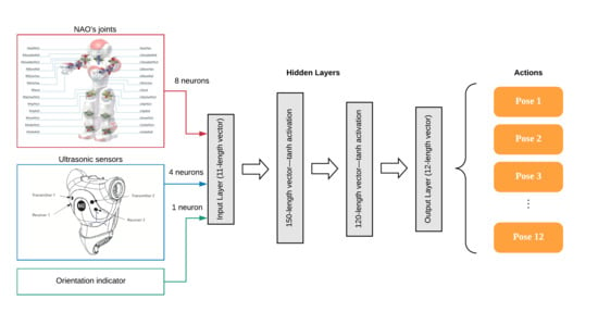
The proposed Q-network in this level is composed of one input layer with 11 neurons, where 8 of them are taken from the joints of the robot: (1) left hip pitch, (2) left knee pitch, (3) left ankle pitch, (4) left ankle roll, (5) right hip pitch, (6) right knee pitch, (7) right ankle pitch, and (8) right ankle roll.
Notice that in this state, we are only considering both legs of the robot, four values for each one; this is again, to reduce the complexity. After some experiments, we found that this information is enough to make the algorithm converge while accomplishing the goal task.
The remaining neurons correspond to the ultrasonic sensors (two neurons) and the indicator of the deviation of the robot. If the robot deviates in an angle of more than 10 degrees to the left or to the right, this indicator value is −1, otherwise the indicator gives a value of +1.
The proposed net has two hidden layers, the first one has 150 neurons with a tanh activation function, and in the second hidden layer, there are 120 neurons with the same tanh activation function.
Finally, an output layer of 12 neurons with the activation function ReLU (rectifier linear unit) is created, with each of the neurons corresponding to one action. In this level, the actions available are the poses that were learned before; remember in the first layer the system learned 12 poses, so these are the available actions for this level. This architecture is shown in Figure 8.
4. Experiment and Results
This section begins with a brief overview of the software used for simulating and training the networks used in this method. Afterwards, details of our fall module to detect if a robot fell down or not are given. To finish this section, we show the results of training the robot to walk, we compare the speed reached with the speed of the NAO built-in walking controller, and we show the results of training changing a parameter called action time and its effects in the performance of the system (the implementation of our neural network, as well as interface with the simulator environment, can be found at http://idic.likufanele.com/~calvo/gait/).
4.1. Simulation Software
Following the recent trend of finding optimal parameters in simulated environments, to avoid costly experiments in terms of time and physical wear [32,33], we use a simulator software called Webots (http://www.cyberbotics.com). Webots is a development environment used to model, program, and simulate mobile robots [34]. With Webots, the user can design complex robotic setups, with one or several similar or different robots in a shared environment. The properties of each object, such as shape, color, texture, mass, friction, etc., are chosen by the user. A large choice of simulated sensors and actuators is available to equip each robot.
Webots allows for the launch of a simulated NAO moving in a virtual world (for details, see http://doc.aldebaran.com/1-14/software/webots/webots_index.html). This simulator is a convenient choice because in this simulator we can read all the sensors of the robot, the force sensors to compute the ZMP, the joints sensors that give us the real value of the joints, the ultrasonic sensor we need to measure the distance covered, etc. (refer to Figure 9). The simulator allows the user to interface with C, C++, and Python. In the environment, we can add multiple obstacles and we can even access the cameras of the NAO.
4.2. Q-Network Algorithm
To communicate with the NAO robot, we use the NAOqi Framework (for details, see http://doc.aldebaran.com/2-1/ref/index.html). NAOqi is the name of the main software that runs on the robot and controls it. The NAOqi Framework is the programming framework used to program NAO. It answers to common robotics needs including: parallelism, resources, synchronization, and events. This framework allows homogeneous communication between different modules (motion, audio, and video), homogeneous programming, and homogeneous information sharing (see http://doc.aldebaran.com/1-14/dev/naoqi/index.html#naoqi-framework-overview).
4.2.1. Programming Environment
The whole program is written in Python 2.7 with a Python Application Programming Interface (API) developed by Aldebaran robotics to communicate with the NAOqi framework.
We designed and trained the artificial neural networks with the Python library Keras; this is a high-level neural network API, written in Python, and is capable of running on top of either TensorFlow or Theano. It was developed with a focus on enabling fast experimentation (retrieved from https://keras.io/).
The library contains numerous implementations of commonly used neural network building blocks such as layers, objectives, activation functions, optimizers, and a lot of tools to make working with images and text data easier. From these, we selected and loaded only the required modules in order to have an efficient use of memory.
Each time a new action is taken, the reward that this action yields must be evaluated and the model is trained again based on this information. Because of this, Graphical Processing Unit (GPU)-optimization is needed. We use the Keras backend with Theano to take advantage of the GPU of the NVIDIA Geforce GTX 580; otherwise, we would not have been able to compute the results fast enough. The motors of the NAO take 0.1 seconds to complete a movement instruction, while computing the update of a Q-network using the Central Processing Unit (CPU) took approximately 2 seconds (this was implemented on an Intel Core i5 computer with 8 GB of RAM; see Figure 10). Evidently, this is not fast enough. Fortunately, using the GPU, we could compute the network update in around 0.002 seconds (see Figure 11).
4.2.2. Fall Module
A key element in the algorithm is the capacity to detect the falling of a robot with the fall module. This module is a pre-trained MLP that allows one to identify whether the robot has fallen or not. Even when the NAO robot comes with a built-in module of this type, the answer is very slow, as it provides an answer in 3 seconds, while we needed it in less than 0.2 seconds. This is why the development of a new fall module was needed.
In order to implement this module, we acquired data from the simulation and store in a dataset of 790 values, and we used that data in a previously labeled format to train a Multi-Layer Perceptron (MLP) with an input layer of ten neurons; from these ten neurons, eight belonged to the force sensors in the soles of the feet, and the other two belonged to the inertial unit of the NAO robot. This inertial unit told us the torso angle of the robot with respect to the ground; it was computed using the accelerometer and the gyrometer of the NAO (see Figure 12).
The fall-module MLP has two hidden layers, one with twelve neurons with the ReLU activation function, and another with eight neurons with a sigmoid activation function. Lastly, there was an output layer with only one neuron, which outputs 0 if the robot fell down or 1 if it did not. This architecture is shown in Figure 13.
4.2.3. Algorithm Description
First, we need to load the fall module to detect if the robot has fallen (see Figure 14). Every time the simulated robot fell down, we needed to restore the simulation manually because the simulated robot could not rise by itself. For this reason, we could not train the Q-network in one run; however, we needed to keep training the network just after the last run. For this reason, we needed to save the network model at the end of each run and to load it at the beginning of each new run.
We needed to initialize the NAO proxies, the motion proxy that allows to send signals to the NAO motors; the posture proxy that allows one to set the robot in a “home position”; the sonar proxy, which tells us the information of the ultrasonic sensors; and the memory proxy to access the data recorded, v. gr. the angle of the joints. After that, the robot required activation. We could do this by setting the stiffness of the body to 1—this was achieved using the instruction motion.setStiffnesses (“Body”, 1.0).
We initialized the number of epochs to 50. Notice that we need many more iterations due to the fact that when the robot falls down, it cannot always stand up by itself, and the simulation has to be restored manually. For instance, imagine we set the number of epochs to 2000 and the robot fell down in the second iteration, then we would have to wait until the 2000th iteration to restore the simulation, which would take considerably more time.
Afterwards, we initialized gamma to 0.9, which means experience is considered, the closer gamma to zero, the less we take into consideration the experience of previous trials.
In Reference [31], the authors used a technique to let the algorithm converge via experience replay. It works in the following way: During the run of the algorithm, all the experiences < st, a, r, st+1 > are stored in a replay memory. When training the network, random mini batches from the replay memory are used instead of the most recent transition. Before training we needed to define a variable for this purpose with replay as an empty list; however, as we were running the algorithm multiple times, in our case it is not an empty list, but it was the list previously filled in a previous run, i.e., replay = lastreplay.
We opened a loop from i = 0 until i = epochs, set the robot in the “home position,” which was the NAO posture “StandInit,” then we read sonars with the memory proxy and stored it in sonar. We then read the state; remember that the state in the first level will be a vector of 4 values while in the second level is a vector of 11 values.
Then, we opened a while loop with the condition that the NAO had not reached a terminal state. A terminal state was when the robot fell or when it reached the goal; that is, in the first level a ZMP was located in a specific interval, and in the second level, a distance of 8 cm was covered.
Later, we ran the Q-network forward and stored the result in qval (a vector). Suppose that we have the vector (1.2, −0.36, 2.2, 0.0). The actiont+1 will be the action 3 because the third value is the greatest; however, we wanted to explore more options in order to not fall in a local minimum, so with a probability of epsilon, we chose between the max action or a random action. This epsilon gradually decreased in such a way that after many iterations it became 0.
Then, we applied the actiont+1 and observed the reward and the new state, where the values of the reward were described in the previous section. At this point, we had [state, action, reward, new state]. We needed to store this tuple in replay and repeat the process until the length of replay was the same as buffer; we set buffer as 60. Once the buffer was filled, we got a mini batch, which was a random sample of length 30 from the replay array.
Thereafter, we looped over each element of the mini batch. Each element was a list of four values that we used to set (old state, action, reward2, new state2), then we ran forward our Q-network using as input the old state and stored the result in old qval, where we selected the greatest value of old qval and saved the index of it in maxQ. Later, we defined a vector X with the same values of old state, and a vector Y with the same values of old qval.
At this point, we needed to check whether the reward2 belonged to a terminal state, i.e., if the variable update was equal to the value of the reward2; if not, update = (reward2 + (gamma × maxQ)). This variable update was the rule used to compute the update of the neural network.
The value of the variable update needed to replace the value in the Y vector in the position of index. For instance, suppose we have a Y = [1.2, −0.36, 2.2, 0.0], index = 3, and update = 10, such that the result after replacing is Y = [1.2, −0.36, 10, 0.0]. This will be the target for the Q-network, which should be done for all the elements in the minibatch. Once we finished the loop, we used the entire Y and X vector to train the Q-network using backpropagation. The Q-network algorithm is shown in Figure 15.
4.3. Learning the Poses
During the first level of training, the results we got were the configurations of the joints that we had previously defined as poses. The results are presented in Table 2, showing the value of the degrees of each joint. These values rendered the pose shown in Figure 16. Note that some angles remain fixed, such as the head pitch and yaw.
| Left Arm | Right Arm | ||
| L Shoulder Pitch | 105.20 | R Shoulder Pitch | 105.08 |
| L Shoulder Roll | 15.69 | R Shoulder Roll | −15.31 |
| L Elbow Yaw | −85.87 | R Elbow Yaw | 85.85 |
| L Elbow Roll | −29.59 | R Elbow Roll | 29.72 |
| L Wrist Yaw | 0.00 | R Wrist Yaw | 0.00 |
| Left Leg | Right Leg | ||
| L Hip Yaw Pitch | 0.00 | R Hip Yaw Pitch | 0.00 |
| L Hip Roll | 2.87 | R Hip Roll | 2.87 |
| L Hip Pitch | −18.51 | R Hip Pitch | −18.51 |
| L Knee Pitch | 48.04 | R Knee Pitch | 48.04 |
| L Ankle Pitch | −29.53 | R Ankle Pitch | −29.53 |
| L Ankle Roll | −6.33 | R Ankle Roll | −6.33 |
4.4. Learning to Walk
It was then time to learn the activity of walking. This was done using the previously learned knowledge, i.e., the poses. In the previous sections, we described the use of Q-networks to learn to walk, the state as defined by the combination of some selected robot joints, the value of the ultrasonic sensor, and an additional value that identified whether the robot was deviating or not.
The actions for the network are the poses, and by this moment, the system had already deduced the angle of each joint of the robot to achieve the 12 proposed poses and the reward was given by the distance advanced (the goal was to reach 8 centimeters).
The Q-network proposed in the methodology remained the same: a 4-layer Multi-Layer Perceptron (MLP), with one input layer of 11 neurons; 2 hidden layers, both with tanh activation function; one with 150 neurons and other with 120 neurons; and finally, an output layer with 12 neurons, one for each pose.
The algorithm was tested in a simulated NAO robot on the Webots simulator, having in mind that the motors response was approximately 0.08 seconds, the actions performed by the algorithm were set to 0.1s. In other words, we chose a pose of the 12 available, then we sent the signal to the motor, but the result would not be reflected until 0.08 s later; we had to wait this time so that we could read the new state and the reward. This waiting time between actions is called the action time.
Even when it was first thought the action time would always be 0.1 s, we realized that modifying this action time would have an effect in the performance of the algorithm. For this reason, the algorithm was tested using different values of the action time (0.1 s, 0.15 s, 0.2 s, and 0.25 s).
The four tests were done in the same conditions, with the goal distance being 8 cm, and the available actions for the Q-network, the 12 poses, and the size of the Q-network were also the same.
4.4.1. Results for an Action Time of 0.1 s
The first test was using an action time of 0.10 s. It took around 2500 iterations to converge. The poses chosen for the algorithm in this test were pose 10, pose 1, pose 3, pose 4, pose 7, pose 7, pose 8, and pose 12, as illustrated in Figure 17. The robot, following these poses, took on average 1.621 s to reach the 8 centimeters marked as the goal.
4.4.2. Results with an Action Time of 0.15 s
The next test used an action time of 0.15 s. It took around 2800 iterations to converge, where the poses chosen for the algorithm in this test were pose 1, pose 3, pose 4, pose 7, and pose 12, as illustrated in Figure 18. The robot, following these poses, took an average of 1.520s to reach the 8 centimeters marked as the goal.
4.4.3. Testing with an Action Time of 0.2 s
The next test used an action time of 0.20 s. It took around 2500 iterations to converge. The poses chosen for the algorithm in this test were the same that the test before: pose 1, pose 3, pose 4, pose 7, and pose 12; however, in this case, the robot took 2.2 s on average to reach the 8 centimeters marked as the goal.
4.4.4. Testing with an Action Time of 0.25 s
The last test used an action time of 0.25 s. It took around 2600 iterations to converge. The poses chosen for the algorithm in this test were pose 1, pose 4, pose 7, and pose 12. The robot, using these poses, took 2.015 s on average to reach the 8 centimeters marked as the goal. See Figure 19.
Comparing the performance of the four tests we have, the fastest one was the test done with the action time of 0.15 s, and the slowest was the one with the action time of 0.2 s.
A comparison table of the four tests is shown in Table 3.
4.4.5. Comparing Results
The NAO robot came with a built-in controller based on an inverted pendulum to control the gait cycle, and we could configure the speed of the NAO with this controller. Normally, the NAO reached a speed of 3.92 cm/s; however, in fast walking mode, it could reach a speed of 6.153 cm/s (see Table 4).
When comparing the result of the four tests with the normal speed of the NAO, we can see that tests with action times of 0.15 s and 0.1 s were faster than the normal speed of the robot. Furthermore, the test with an action time of 0.25 s was still slightly better. These results are encouraging because the performance was enough to be considered as a good performance.
Nevertheless, when comparing with the fast walking mode of the NAO, none of the four tests was faster than the NAO’s built-in fast walking, the closest one being the test with the action time of 0.15 s. However, when testing whether the robot fell down or not, when we tested the resultant Q-networks during 10 tests of 5 s each, the robot never fell down; however, when testing the NAO’s built-in fast walking, in 3 out of 10 tests done with that speed, the robot fell down (the comparison of stability and deviation between the normal walking and fast walking of the NAO, as well as the four obtained results, can be analyzed in detail in Video S1; see Figure 20).
5. Conclusions and Future Work
In this section, we summarize the results and conclusions obtained in this work, as well as the analysis about stability and the ability to not fall down. Later, there is an explanation of how we believe the definitions of the action, state, and reward can be applicable to other robots. Afterwards we expose why the learning framework can be considered successful. Finally, future work directions are discussed.
5.1. Stability and Not Falling Down
After training the whole system, the robot was able to walk while displaying a stable behavior, which was to walk with balance. In addition, the robot did walk in straight line, i.e., it did not deviate. On the other hand, the algorithm provided for the robot allowed us to find: (i) a collection of twelve poses based on a ZMP criterion, and (ii) a combination of these poses in different action times that allow the robot to reach the goal distance without falling down and without deviating. Allowing the robot to avoid falling down is a very important part of this work and during the experimentation we found that our approach accomplished this objective.
5.2. Actions, States, and Rewards Applicable to Other Robots
The state of the first level of the learning framework was obtained from the four force-sensors in each foot in such a way that this definition of state will work for every robot that has these kinds of sensors.
The state of the second level was formed with the information of the current angle of the joints and the value of the ultrasonic sensors of the robot. If a robot had the opportunity to read the angle of its joints and there was a readable value of the sensors that measured the distance, then the definition of the state in this level was applicable for that robot.
The reward of the first level was computed depending on the region where the ZMP was. Therefore, for any robot that had the force sensors on its feet, we would be able to use the same reward definition for this level.
The reward of the second level was computed using the values of the ultrasonic sensors, that is, the measure of the distance. Because of this, in any robot in which we could measure the distance, we could apply the same definition of reward.
On the first level of the Q-network, the available actions proposed here were modules that interacted directly with the current position of a joint, and they increased or decreased the value of a joint. For that, if we could send a command to a robot that modified the position of a joint of that robot, then we could use this definition of actions for that robot.
On the second level of the Q-network, the actions are the poses that the learning framework previously learned; therefore, if we could apply the Q-network of the first level on a robot and it succeeded, then that robot may be able to learn and to use the poses of the first level. The actions were the same proposed here; of course, the poses were not expected to be the same but the way they were learned and how they are used can be the same as in this work.
5.3. Learning Framework
At the end of this work, we verified that the approach proposed here works using the same machine learning technique (q-learning) such that we could induce the poses that conformed to the first level of our hypothetical learning framework, and we could make the robot walk just by combining these poses.
We showed that with this algorithm, it was not necessary to consider the kinematics of the robot, and it was unnecessary to compute the inverse kinematics of the joints since we just have to know the information of some sensors to deduce some modules that we called poses to further used them in a more complex activity. The convergence time of the algorithm in each pose and in each walking test was large, but the results were satisfying.
It is clear that the approach is far from perfect, even when comparing the results with the built-in build of the robot showing that performance was good, there were many scenarios where this algorithm failed because in this work we have only considered a specific setting for walking, that is, walking in straight line on a flat floor. If we tried the algorithm as it is on a ramp, this will lead to the robot falling down.
Additional settings for walking and the possibility of expanding the number of activities at level two to achieve a task of level three in the learning framework is what leads us to describe the future work.
5.4. Future Work
On one hand, we can explore different stages of walking, that is, walking on an irregular floor, walking on ramps, or omnidirectional walking, i.e., to walk in any direction, not only in a straight line. On the other hand, we can keep adding activities, i.e., modules of level two of the learning framework. Until now, we have proposed and tested only one activity, i.e., walking, but the idea is to learn more activities. Of course, more poses are needed to achieve such new activities. For instance, we can add “sit down,” “turn around,” or “take an object.” Lastly, to transfer the simulated algorithm to physical robots is left as future work.
Once our system has more activities available, we can ask the system to learn a module of level three; remember that we defined these modules as tasks, so the next step will be to learn a task just by using the previous information, i.e., the activities.
Supplementary Materials
The following are available online at https://www.mdpi.com/2076-3417/9/3/502/s1, Video S1: Comparing NAO walking modes.
Author Contributions
Conceptualization: C.R.G. and H.C.; Methodology: C.R.G., H.C. and H.S.; Software: C.R.G.; Investigation: H.C.; Writing: H.C. and C.R.G.; Supervision: H.S.
Funding
This research was funded by CONACyT-SNI, Fronteras de la Ciencia 65, and Instituto Politecnico Nacional (IPN), particularly through grants SIP20182114, SIP20180730, SIP20190007, 20195886, EDI, and COFAA-SIBE.
Conflicts of Interest
The authors declare no conflict of interest.
References
- Shirashaka, S.; Machida, T.; Igarashi, H. Leg Selectable Interface for Walking Robots on Irregular Terrain. In Proceedings of the 2006 SICE-ICASE International Joint Conference, Busan, Korea, 18–21 October 2006. [Google Scholar]
- Ill-Woo, P.; Jung-Yup, K.; Jungho, L. Online Free Walking Trajectory Generation for Biped. In Proceedings of the IEEE Internactional Conference on Robotics and Automation (ICRA 2006), Orlando, FL, USA, 15–19 May 2006; pp. 1231–1236. [Google Scholar]
- Huang, Q.; Kajita, S.; Koyachi, N.; Kaneko, K.; Yokoi, K.; Kotoku, T.; Arai, H.; Komoriya, K.; Tanie, K. Walking patterns and actuator specifications for a biped robot. In Proceedings of the 1999 IEEE/RSJ International Conference on Intelligent Robots and Systems. Human and Environment Friendly Robots with High Intelligence and Emotional Quotients (Cat. No.99CH36289), Kyongju, Korea, 17–21 October 1999. [Google Scholar]
- Tay, A.B. Walking Nao Omnidirectional Bipedal Locomotion. Bachelor’s Thesis, Bachelor of Science, School of Computer Science and Engineering, The University of New South Wales, Kensington, UK, 2009; pp. 1–49. [Google Scholar]
- Morimoto, J.; Cheng, G.; Atkeson, C.G.; Zeglin, G. A simple reinforcement learning algorithm for biped walking. In Proceedings of the IEEE International Conference on Robotics and Automation, 2004. Proceedings. ICRA ‘04. 2004, New Orleans, LA, USA, 26 April–1 May 2004. [Google Scholar]
- Jin-Ling, L.; Kao-Shing, H.; Wei-Cheng, J.; Yu-Jen, C. Gait Balance and Acceleration of a Biped Robot. IEEE Access 2016, 4, 2439–2449. [Google Scholar]
- Michel, O. Webots: Symbiosis between virtual and real mobile robots. In International Conference on Virtual Worlds; Lecture Notes in Computer Science 1434; Springer: Berlin/Heidelberg, Germany, 1998; pp. 254–263. [Google Scholar]
- Hubicki, C.; Abate, A.; Clary, P.; Rezazadeh, S.; Jones, M.; Peekema, A.; Van Why, J.; Domres, R.; Wu, A.; Martin, W.; et al. Walking and running with passive compliance: Lessons from engineering a live demonstration of the ATRIAS biped. IEEE Robot. Autom. Mag. 2018, 25, 23–39. [Google Scholar] [CrossRef]
- Martin, W.C.; Wu, A.; Geyer, H. Robust spring mass model running for a physical bipedal robot. In Proceedings of the 2015 IEEE International Conference on Robotics and Automation (ICRA), Seattle, WA, USA, 26–30 May 2015; pp. 6307–6312. [Google Scholar]
- Hong, S.; Kim, E. A New Automatic Gait Cycle Partitioning Method and Its Application to Human Identification. Int. J. Fuzzy Log. Intell. Syst. 2007, 17, 51–57. [Google Scholar] [CrossRef]
- Jung-Yup, K.; Ill-Woo, P.; Jun-Ho, O. Walking Control Algorithm of Biped Humanoid Robot on Uneven and Inclined Floor. J. Intell. Robot. Syst. 2007, 48, 457–484. [Google Scholar] [Green Version]
- Huang, Q.; Yokoi, K.; Kajita, S.; Kaneko, K.; Arai, H.; Koyachi, N.; Tanie, K. Planning Walking Patterns for a Biped Robot. IEEE Trans. Robot. Autom. 2001, 17, 280–289. [Google Scholar] [CrossRef]
- Lu, Q.; Zheng, Y.; Lu, X. Deviation Correction Control of Biped Robot Walking Path Planning. In IOP Conference Series: Materials Science and Engineering; IOP Publishing: Bristol, UK, 2018; Volume 394, p. 032029. [Google Scholar]
- Ito, S.; Nishio, S.; Ino, M.; Morita, R.; Matsushita, K.; Sasaki, M. Design and adaptive balance control of a biped robot with fewer actuators for slope walking. Mechatronics 2018, 49, 56–66. [Google Scholar] [CrossRef]
- Liu, C.; Yang, J.; An, K.; Chen, Q. Rhythmic-Reflex Hybrid Adaptive Walking Control of Biped Robot. J. Intell. Robot. Syst. 2018, 7, 1–17. [Google Scholar] [CrossRef]
- Righetti, L.; Jan Ijspeert, A. Programmable Central Pattern Generators: An application to biped locomotion control. In Proceedings of the IEEE International Conference on Robotics and Automation, Orlando, FL, USA, 15–19 May 2006; pp. 1585–1590. [Google Scholar]
- Liu, J.; Chen, X.; Veloso, M. Simplified walking: A new way to generate flexible biped patterns. In Mobile Robotics: Solutions and Challenges; World Scientific: Singapore, 2010; pp. 583–590. [Google Scholar]
- Rivas, F.M.; Canas, J.M.; González, J. Automatic learning of walking modes for a humanoid robot (in Spanish). In Proceedings of the Robot2011 III Robotics Workshop, Experimental robotics, Seville, Spain, 28–29 November 2011; pp. 120–127. [Google Scholar]
- Meriçli, Ç.; Veloso, M. Biped walk learning on NAO through playback and real-time corrective demonstration. Workshop on Agents Learning Interactively from Human Teachers. In Proceedings of the 9th International Conference on Autonomous Agents and Multiagent Systems (AAMAS 2010), Toronto, ON, Canada, 9–14 May 2010. [Google Scholar]
- Kao-Shing, H.; Keng-Hao, Y.; Jia-Yan, L. The Study on the Learning of Walking Gaits for Biped Robots. Int. Fed. Autom. Control 2013, 46, 589–593. [Google Scholar]
- Gasparri, G.M.; Manara, S.; Caporale, D.; Averta, G.; Bonilla, M.; Marino, H.; Catalano, M.; Grioli, G.; Bianchi, M.; Bicchi, A.; et al. Efficient Walking Gait Generation via Principal Component Representation of Optimal Trajectories: Application to a Planar Biped Robot with Elastic Joints. IEEE Robot. Autom. Lett. 2018, 3, 2299–2306. [Google Scholar] [CrossRef]
- Corral, E.; Marques, F.; García, M.J.G.; Flores, P.; García-Prada, J.C. Passive walking biped model with dissipative contact and friction forces. In European Conference on Mechanism Science; Springer: Cham, Switzerland, 2019; pp. 35–42. [Google Scholar]
- Dekker, M. Zero-Moment Point Method for Stable Biped Walking; University of Technology: Eindhoven, The Netherlands, 2009. [Google Scholar]
- Strom, J.; Slavov, G.; Chown, E. Omnidirectional Walking Using ZMP and Preview Control for the NAO Humanoid Robot. Lect. Notes Comput. Sci. 2010, 5949, 378–389. [Google Scholar]
- Lee, H.W.; Yang, J.L.; Zhang, S.Q.; Chen, Q. Research on the Stability of Biped Robot Walking on Different Road Surfaces. In Proceedings of the 2018 1st IEEE International Conference on Knowledge Innovation and Invention (ICKII), Jeju, Korea, 23–27 July 2018; pp. 54–57. [Google Scholar]
- Van der Noot, N.; Barrera, A. Zero-Moment Point on a Bipedal Robot. In Proceedings of the 17th IEEE Mediterranean Electrotechnical Conference, Beirut, Lebanon, 13–16 April 2014. [Google Scholar]
- Liu, Y.; Zang, X.; Zhang, N.; Liu, Y.; Wu, M. Effects of unilateral restriction of the metatarsophalangeal joints on biped robot walking. In Proceedings of the 2018 Eighth International Conference on Information Science and Technology (ICIST), Cordoba, Spain, 30 June–6 July 2018; pp. 395–400. [Google Scholar]
- Duysens, J.; Forner-Cordero, A. Walking with perturbations: A guide for biped humans and robots. Bioinspir. Biomim. 2018, 13, 061001. [Google Scholar] [CrossRef] [PubMed]
- Kao-Shing, H.; Jin-Ling, L.; Jhe-Syun, L. Biped Balance Control by Reinforcement Learning. J. Inf. Sci. Eng. 2016, 32, 1041–1060. [Google Scholar]
- McGinnis, P.M. Biomechanics of Sport and Exercise; Human Kinetics Publishers: Champaign, IL, USA, 2015. [Google Scholar]
- Mnih, V.; Kavukcuoglu, K.; Silver, D.; Graves, A. Playing Atari with Deep Reinforcement Learning. arXiv, 2013; arXiv:1312.5602. [Google Scholar]
- Singla, A.; Bhattacharya, S.; Dholakiya, D.; Bhatnagar, S.; Ghosal, A.; Amrutur, B.; Kolathaya, S. Realizing Learned Quadruped Locomotion Behaviors through Kinematic Motion Primitives. arXiv, 2018; arXiv:1810.03842. [Google Scholar]
- Rai, A.; Antonova, R.; Meier, F.; Atkeson, C.G. Using Simulation to Improve Sample-Efficiency of Bayesian Optimization for Bipedal Robots. arXiv, 2018; arXiv:1805.02732. [Google Scholar]
- Michel, O. Webots: Professional Mobile Robot Simulation. Int. J. Adv. Robot. Syst. 2004, 1, 39–42. [Google Scholar] [CrossRef]
Figure 1.
Zero Moment Point (ZMP) concept (CoM is the center of mass).

Figure 2.
Learning activities for robots using a decomposition framework.

Figure 3.
NAO’s hello gesture decomposition.

Figure 4.
Walking learning framework.

Figure 5.
Poses 1 to 6.

Figure 6.
Poses in one-foot sole.

Figure 7.
First Level Q-Network.

Figure 8.
Second Level Q-network.

Figure 9.
Webots for NAO.

Figure 10.
Training Time using a Central Processing Unit (CPU).

Figure 11.
Training Time using a Graphical Processing Unit (GPU).

Figure 12.
NAO Inertial Unit.

Figure 13.
Fall Module Multi-Layer Perceptron (MLP).

Figure 14.
NAO trying to stand up and failing.

Figure 15.
Q-network Algorithm.

Figure 16.
Pose 1.

Figure 17.
Selected poses for an Action Time of 0.1 s.

Figure 18.
Selected Poses for an Action Time of 0.15 s.

Figure 19.
Selected poses for an Action Time of 0.2 s.

Figure 20.
NAO in fast walking mode that had fallen down.


Table 1.
Base-level movements, range of movement, and limitations selected in this work.
| No. | Movement | NAO Joint (in °) | Limit (in °) | ||
|---|---|---|---|---|---|
| From | To | From | To | ||
| 1 | Left shoulder pitch | −119.50 | 119.50 | 70.00 | 110.00 |
| 2 | Left elbow roll | −88.50 | −2.00 | −65.00 | −25.00 |
| 3 | Left, hip pitch | −88.00 | 27.73 | −35.00 | −15.00 |
| 4 | Left knee pitch | −5.29 | 121.04 | 45.00 | 65.00 |
| 5 | Left ankle pitch | −68.15 | 52.86 | −45.00 | −25.00 |
| 6 | Right shoulder pitch | −119.50 | 119.50 | 70.00 | 110.00 |
| 7 | Right elbow roll | −88.50 | −2.00 | −65.00 | −25.00 |
| 8 | Right hip pitch | −88.00 | 27.73 | −35.00 | −15.00 |
| 9 | Right knee pitch | −5.29 | 121.04 | 45.00 | 65.00 |
| 10 | Right ankle pitch | −68.15 | 52.86 | −45.00 | −25.00 |
Table 2.
Angles of Pose 1.
| Head | |
|---|---|
| Head Pitch | 0 |
| Head Yaw | 0 |
Table 3.
Q-network Results.
| Q-Network Results | |||||
|---|---|---|---|---|---|
| Action Time | Number of Poses | List of Poses | Distance | Time | Speed |
| 0.10 s | 8 | 10, 1, 3, 4, 7, 7, 8, 12 | 8 cm | 1.621 s | 4.93 cm/s |
| 0.15 s | 5 | 1, 3, 4, 7, 12 | 8 cm | 1.520 s | 5.26 cm/s |
| 0.20 s | 5 | 1, 3, 4, 7, 12 | 8 cm | 2.200 s | 3.63 cm/s |
| 0.25 s | 4 | 1, 4, 7, 12 | 8 cm | 2.015 s | 3.97 cm/s |
Table 4.
NAO’s built-in walking controller.
| NAO Built-In Walking Controller | |||
|---|---|---|---|
| Mode | Distance | Time | Speed |
| Normal Walking | 8 cm | 2.04 s | 3.92 cm/s |
| Fast Walking | 8 cm | 1.30 s | 6.153 cm/s |
© 2019 by the authors. Licensee MDPI, Basel, Switzerland. This article is an open access article distributed under the terms and conditions of the Creative Commons Attribution (CC BY) license (http://creativecommons.org/licenses/by/4.0/).
Share and Cite
MDPI and ACS Style
Gil, C.R.; Calvo, H.; Sossa, H. Learning an Efficient Gait Cycle of a Biped Robot Based on Reinforcement Learning and Artificial Neural Networks. Appl. Sci. 2019, 9, 502. https://doi.org/10.3390/app9030502
AMA Style
Gil CR, Calvo H, Sossa H. Learning an Efficient Gait Cycle of a Biped Robot Based on Reinforcement Learning and Artificial Neural Networks. Applied Sciences. 2019; 9(3):502. https://doi.org/10.3390/app9030502
Chicago/Turabian StyleGil, Cristyan R., Hiram Calvo, and Humberto Sossa. 2019. "Learning an Efficient Gait Cycle of a Biped Robot Based on Reinforcement Learning and Artificial Neural Networks" Applied Sciences 9, no. 3: 502. https://doi.org/10.3390/app9030502
Note that from the first issue of 2016, this journal uses article numbers instead of page numbers. See further details here.