Cutting Insert and Parameter Optimization for Turning Based on Artificial Neural Networks and a Genetic Algorithm


1
Department of Mechanical and Electrical Engineering, National Taipei University of Technology, Taipei 10608, Taiwan
2
Department of Mechanical and Automation Engineering, National Taipei University of Technology, Taipei 10608, Taiwan
3
Department of Mechanical Engineering, National Taipei University of Technology, Taipei 10608, Taiwan
*
Author to whom correspondence should be addressed.
Appl. Sci. 2019, 9(3), 479; https://doi.org/10.3390/app9030479
Submission received: 2 January 2019
/
Revised: 25 January 2019
/
Accepted: 28 January 2019
/
Published: 30 January 2019
(This article belongs to the Special Issue New Industry 4.0 Advances in Industrial IoT and Visual Computing for Manufacturing Processes)
Abstract
:Featured Application
People and companies involved on the manufacturing industry will be able to save plenty of time on the selection of cutting inserts and parameters by implementing and using the optimization system developed in this research.
Abstract
The objective of this present study is to develop a system to optimize cutting insert selection and cutting parameters. The proposed approach addresses turning processes that use technical information from a tool supplier. The proposed system is based on artificial neural networks and a genetic algorithm, which define the modeling and optimization stages, respectively. For the modeling stage, two artificial neural networks are implemented to evaluate the feed rate and cutting velocity parameters. These models are defined as functions of insert features and working conditions. For the optimization problem, a genetic algorithm is implemented to search an optimal tool insert. This heuristic algorithm is evaluated using a custom objective function, which assesses the machining performance based on the given working specifications, such as the lowest power consumption, the shortest machining time or an acceptable surface roughness.

1. Introduction
Nowadays, there is great demand in the manufacturing industry for technologies that can deal with dynamic environments and customized products. Industry 4.0 and the notion of challenging trade by globalization have pushed companies to be more competitive in both large and small batches. This progress also shows a new way for computer numerical control (CNC) manufacturing industries to profit from large productions [1]. During the last few decades, there has been significant progress in improving the efficacy of CNC machining to meet world challenges. These breakthroughs come from the implementation of automation approaches, such as adaptive control and active control. They allow companies to achieve higher operation performances [1]. Manufacturing processes, such as computer-aided process planning (CAPP), expert processes planning systems (PP), computer-aided design (CAD) and computer-aided manufacturing (CAM) are now based on intelligent machining [2,3], which allow for the simulation and evaluation of variable environments. Complex cutting models can now predict fundamental variables related to machining operations performed in the industry [4]. These approaches mainly aim to obtain suitable cutting parameters and control them within certain working conditions. Thus, this increases the efficiency during the machining process and reduces the implementation time.
Cutting parameters for machining processes have a high impact on performance and they are usually the variables that need to be tuned for optimizing models. Generally, cutting parameters refer to cutting velocity, feed rate, depth of cut, cutting forces, torque, spindle speed, etc. On the other hand, the parameters for evaluating the machining results normally include surface roughness, power consumption, machining time, production cost, tool life, production rate, etc. [5,6,7]. For machining processes, accurate performance can be defined only within a working optimal range. This optimal range is evaluated by models, which generally relate the working conditions to cutting parameters and tool features. These models can be numeric, analytic, empiric, hybrid or AI-based models [4]. Nowadays, the trend is to use AI-based models, which clearly show adaptability and high performance in machining operations. Furthermore, the advances in computer science have allowed for the wide application of these models in the manufacturing industry [8,9,10].
In general, the implementation stage for machining processes takes a considerable amount of time and sometimes requires previous machining tests to reach admissible results. Because of this, some approaches seek to embed knowledge and technical data in machining processes. This results in the development of expert systems that are capable of optimally dealing with the changing conditions in shorter setting times. Many such expert systems use information from CAD models, databases, statement rules, tool preferences, suppliers, etc. [2,3,4,11,12]. Zarkti et al. [3] presented an automatic-optimized tool selector model based on CAD information to infer milling process stages. This approach uses a database from a tool supplier to build an expert system, which is capable of choosing suitable tools and suggesting optimal milling operation planning. Benkedjouh et al. [13] developed a model, which was based on a support vector machine, to predict the life of a cutting tool. This approach uses experimental testing to obtain a nonlinear regression model to estimate and predict the level of wear in a cutting tool. Several sensors, which are installed around the machine, gather information during the machining process and create a database to infer the model. Some significant remarks were taken from Özel et al. [14]. In this present study, the effects of cutting edge geometry on surface hardness are detailed. Moreover, this paper presents the relation between the cutting conditions and the surface roughness for turning processes. In addition, Arrazola et al. [4] detailed several models for chip formation, which can be used to predict cutting forces, temperatures, stress and strain. These models are based on insert geometries and cutting parameters. The approach [12] proposes a system software to optimize cutting parameters based on genetic algorithms. This model defines an objective function, which is based on theoretical models that relate fundamental variables in the machining operation. Ganesh et al. [5] showed an optimization of cutting parameters for the turning process. This research defines the surface roughness as an objective function for turning machining of EN 8 steel. A genetic algorithm is also applied in this approach. This model can be considered to be a hybrid model. Although the study by Li et al. [9] predicts annual power load consumption, the approach also shows an interesting hybrid model based on regression neural networks and the fruit fly optimization algorithm. This research presents a significant improvement in accuracy compared with previous approaches without neural network algorithms. Other models also show important achievements after applying training-based models that use the neural network algorithm. For instance, Xiong et al. [15] used the weld bead geometry prediction; Babu et al. [16] predicted the tensile behavior of tailor weld blanks; and Özel and Karpat [17] presented a model for surface roughness and tool wear for turning operations. Additionally, Malinov et al. [18] created an artificial neural network to predict the mechanical properties of titanium alloys as a function of the alloy composition. The research by Kuo et al. [19] poses a singular model for intelligent stock trading decision support systems. This model captures the stock expert’s knowledge by a genetic-algorithm-based fuzzy neural network model.
Other important achievements for the optimization of cutting parameters have been proposed using only genetic algorithms. Although these approaches show dependency on the working conditions and the workpiece and tools, they can acquire models that can reach the optimal result with high efficiency. In the paper by Quiza Sardinas et al. [20], a multi-objective optimization of cutting parameters in turning operations is presented. This approach entails the use of an objective function based on power consumption, cutting forces and surface roughness. It also presents a qualification of chromosome population, which is inherent to genetic algorithms, based on feasible individuals. Cus and Balic [21] presents an approach for cutting parameters in turning operations. This paper also shows an experimental test for validating the model. Suresh et al. [22] proposes a model to predict surface roughness. This model uses the response surface methodology and a genetic algorithm to converge to an optimal solution. Yang and Tarng [23] showed an approach for optimization of cutting parameters using the Taguchi method and the analysis of variance (ANOVA) for a database obtained by testing surveys. Thamizhmanii et al. [24] presents a similar approach using the Taguchi method and the ANOVA analysis but for optimizing surface roughness.
Unlike other research approaches, our research considers the insert information from a tool supplier to obtain neural network models of insert before determining the optimal cutting parameters. This approach allows the selection of a tool-insert and the inference of the corresponding cutting parameters by simultaneously considering tool specifications and working conditions. To do so, the research is based on a considerable amount of information defined by the tool supplier. The proposed model is an integrated optimization system, which selects a suitable tool-insert and suggests optimal cutting parameters based on certain working conditions and a fitness function optimization, respectively. This approach models the relationships between the geometrical and mechanical features of a tool-insert and the working conditions, thus introducing a novel approach to the modeling of cutting parameters for a turning tool. The output of the proposed approach is a set of recommended cutting parameters for an optimally selected cutting tool. This approach considers the entire information defined by the tool supplier and its intrinsic relationship with the working material in a turning operation. Thus, this makes more assertive recommendations for the cutting parameters.
The objective of this research is to obtain a model for cutting insert selections and cutting parameter optimization. This model must be constrained by working conditions and evaluated by an objective function. The objective function of this approach is defined as a combination of the lowest power consumption, the shortest machining time and surface roughness within a certain range. However, this function must be customizable under external conditions. Furthermore, the cutting insert selection must be based on commercially available tools. Since this research proposes a model for cutting insert selections based on commercially available tools, it requires a database from a tool supplier. The chosen tool supplier was Sandvik Coromant and the selected tool-insert model for building the datasets was CoroTurn® 107. The information about the recommended cutting parameters and the insert feature description was referenced from the official Sandvik Coromant website [25]. The models used on this approach are two artificial neural networks. The first neural network model defines the cutting parameter feed rate as a function of macro-geometrical features and recommended cutting depths. The second model defines the cutting speed as a function of material cutting specifications, working conditions and the feed rate cutting parameter. To find optimal cutting parameters and a suitable cutting insert, a genetic algorithm optimization is proposed based on working conditions. This algorithm is defined by a heuristic search of insert features and cutting parameters, which are evaluated by the neural network models. This heuristic search is set up under a defined objective function, which is a combination of the lowest power consumption, the shortest machining time and an acceptable surface roughness. Due to the heuristic search of the genetic algorithm, the result might be a non-existent tool-insert. Thus, the last stage of this approach is to evaluate a Euclidean distance to find the closest existent tool-insert in the commercial database based on a predefined threshold.
The structure of this paper is as follows. Section 2 aims to introduce the main features that define a tool-insert and the relations of the cutting parameters with geometrical features and the working conditions. This section also defines the database based on commercial data from a tool supplier. The section ends with the proposed dataset for this research. Section 3 explains the procedure used to obtain neural network models for this research. Furthermore, this section introduces data preparation and error validation. Section 4 details the mechanism behind the genetic algorithm implementation. Some concepts, such as individual chromosomes, encoding and decoding procedures and fitness function, are introduced in this section. Section 5 aims to explain how to use this model for practical applications in more detail. Examples of applications shown in this section include light roughing machining, heavy roughing machining and finishing operations. Section 6 summarizes this paper.
2. Datasets Description and Preparation
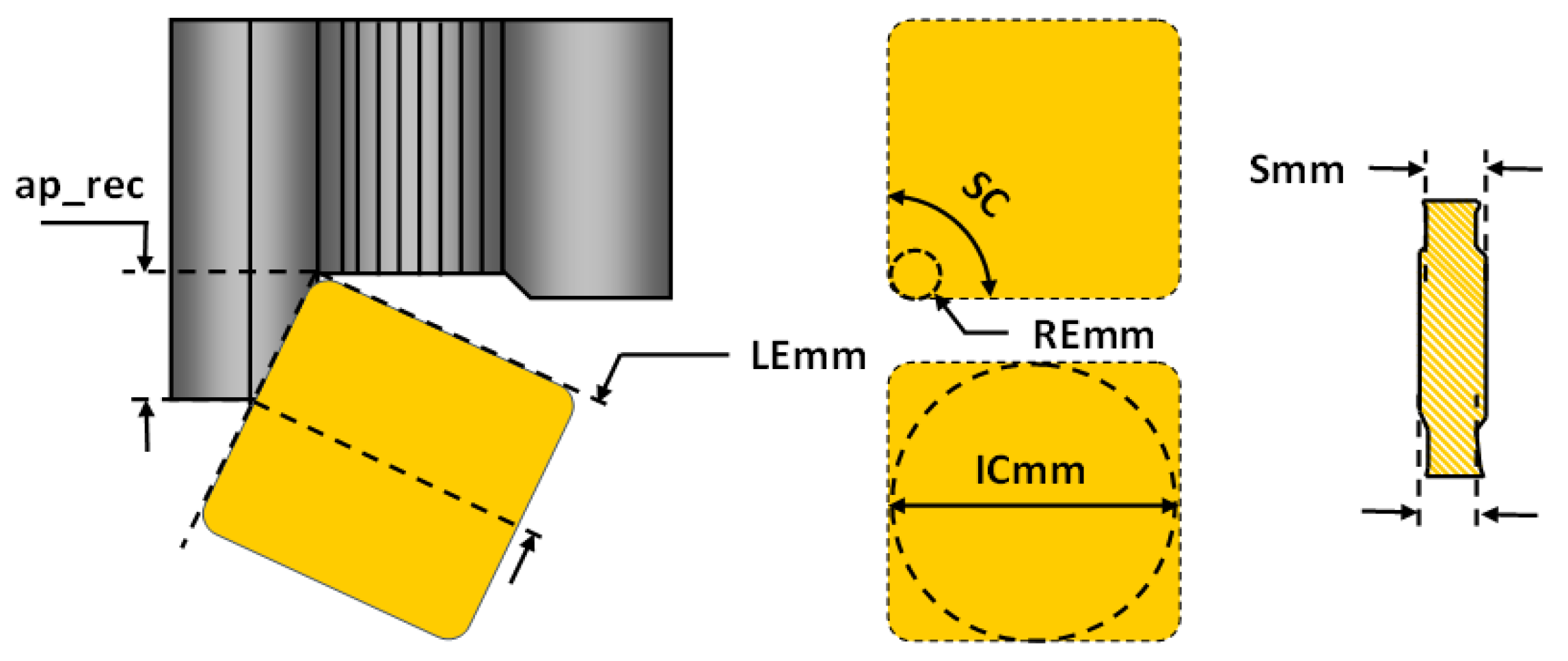
Turning is a process to remove material, which is mainly oriented to metal machining. Within this field, several criteria are used to establish the conditions for an acceptable turning process, including surface roughness, measurement tolerance, power consumption, machining time, forces, loads, etc. These measurement criteria are highly related to the selected cutting insert, cutting parameters, working material and working conditions [25]. A cutting insert varies according to its geometry, shape and material composition. Thus, it is possible to apply a specific group of cutting inserts to a specific turning application, working material and working conditions. In general, a tool-insert can be defined by its geometrical features and material composition, which are hereinafter referred as tool-insert features. The most notable tool-insert features are the inscribed circle (ICmm), clearance angle (AN), cutting length (LEmm), corner radius (REmm), thickness (Smm) and shape angle (SC), as shown in Figure 1.
The ICmm is a tool-insert feature that is highly related to the insert size. A large insert size increases the stability performance but oversizing can lead to high production costs. This feature must be linked with the depth of the cut, the entering angle and the cutting length to be used. The AN is the angle between the front face of the insert and the vertical axis of the workpiece [25]. This feature also defines the negative or positive quality of an insert [25]. On the other hand, the REmm feature is also related to the chip-breaking and cutting forces but it is mainly linked to finished surfaces. For a set feed rate cutting parameter, the machining yields a certain surface roughness. Furthermore, the radial forces that push away the insert in the turning machining become the axial forces as the depth of the cut increases with respect to the radius nose. As a suggestion from the supplier, the depth of cut should be greater or equal to 2/3 of the nose radius of the tool-insert [25]. The insert-shape feature is the most tangible feature, which is mainly selected by accessibility requirements. This feature defines a tool-holder and the depth of cut range in the process. The SC feature is defined by the nose angle of the tool-insert, which is related to strength and reliability issues. Large nose angles are stronger but require more machining power. They also increase the vibration tendency of the machine. On the contrary, small nose angles are weaker and have small cutting edges but are linked to better surface roughness [25].
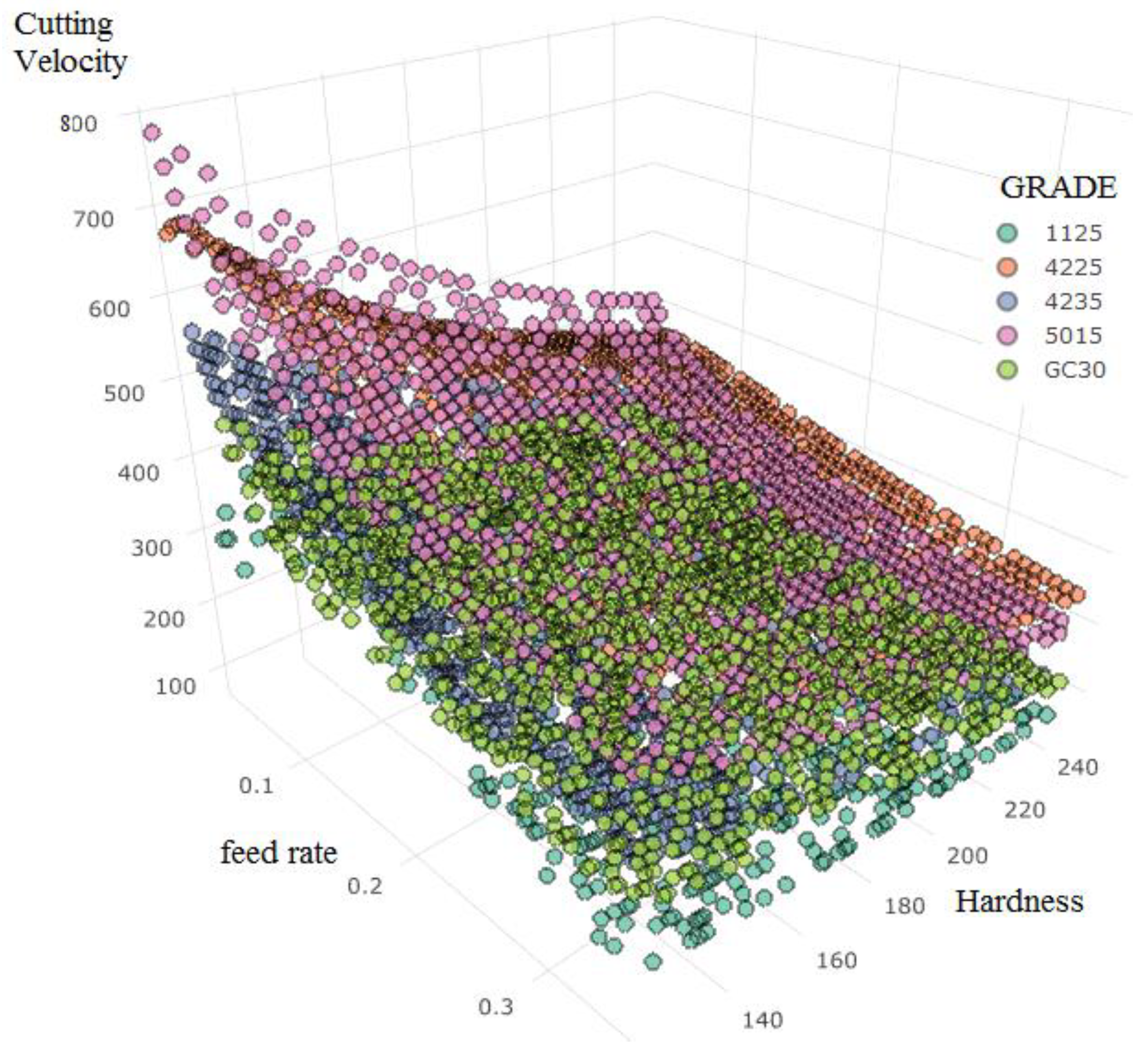
The CTPT feature, which describes the cutting operation, is defined by three possible configurations: Finishing, Medium and Roughing operations. The WEP feature is a logical feature, which defines if the tool insert has a wiper radius. The GRADE feature describes the material composition of a tool-insert. Three features are linked to different grade features. These features describe the distribution of each grade in the range of area applications for ISO group materials. The introduced features are MC_L (machine condition low), MC_H (machine condition high) and MC_Suitability (machine condition suitability). The MC_L and MC_H features represent the low and high borders of each grade in the range of area application. The MC_Suitability feature is defined as a percentage of range for each grade that belongs to wear resistance region, which is in the upper region of the total field of application. For instance, the grade 4325 is defined as MC_L = 40, MC_H = 10 and MC_Suitability = 50%; the grade 5015 is defined as MC_L = 0, MC_H = 20 and MC_Suitability = 100%; and the grade GC30 is defined as MC_L = 35, MC_H = 45 and MC_Suitability = 0% [25]. Figure 2 graphically shows the relation between the working material (hardness feature), cutting parameters (feed rate) and cutting velocity. It is important to note that the relation varies as a function of the insert grade feature.
There are two proposed datasets for this study. The first one is a dataset for insert features with cutting parameters. The second one is for working conditions with cutting parameters. The first dataset will be used to train a neural network model that infers the feed rate while the second one will be used to model the cutting velocity. The description for each dataset is shown in Table 1 and Table 2. The main reason for using two neural network models is the nature of the dataset. The dataset for this study is based on two main sources, which are namely the data description for the tool-insert and the working conditions for a certain working material. The data description for a tool-insert relates the insert features of a tool-insert (i.e., the nose angle, thickness, cutting length and so on) and the suggested cutting parameters (depth of the cut and feed rate). The dataset, which ensues from working conditions, does not relate the insert features to the cutting parameter. It is defined by different working material specifications and their impact on the cutting parameters.
3. Artificial Neural Network Models
An artificial neural network model is a powerful method to deal with nonlinear functions or to model systems with unknown input–output relations [26,27,28]. In fact, the purpose of the algorithm in this research is to find two models that relate the tool-insert features and working conditions to the cutting parameters. Some important issues in the implementation of a neural network model come from the nature of a neural network model. Since a neural network model considers nonlinear combinations and often uses a gradient descent algorithm to update its parameters, the main issues revolve around the need to reach a global solution instead of a local one. Furthermore, given the fact that a neural network model is built on an available dataset, any irrelevant, non-numerical and poor representations of input features can adversely affect the final model [29]. As a machine learning algorithm, neural network models mainly focus on the validation stage. For this reason, the error validation represents proof that the embedded information in the database is well represented by the resulting model. There are some concepts regarding neural network models, which need to be understood. These include overfitting, homogeneous representation and accuracy [30].
For a neural network model, the dataset plays a crucial role. In fact, an effective preparation of the data can lead to an increase in accuracy, reduction in computing time and prevention of overfitting in the model [31]. For the research’s dataset, two scaling methods were considered to prepare the data for the training stage. The independent variables, which define the model inputs, have a scaling method called the z-score. The dependent variables, which describe the output for the neural network model, have a scaling method based on its minimum and maximum values, which has a range from 0 to 1 [31]. Equations (1) and (2) show the z-score and range scaling for inputs and outputs, respectively. It is also important to note that the output for a neural network model is highly dependent on the activation function, which is defined in the last layer (output layer). Generally, the activation function for the last layer is a hyperbolic tangent, softmax or a sigmoid function, which has an output range of 0 to 1. Other activation functions are widely used for neural network models although this research uses a linear function because it can be easily implemented with less computational burden.
The architecture and error validation of a neural network model are closely linked with each other. In fact, the performance of a neural network model is defined by its architecture, but this last one is selected by error validation. The architecture refers to the set of parameters that govern the complexity of the model, including the number of neurons, layers, updating and regularization algorithms among others. The error validation refers to an evaluation procedure for a certain architecture to find a balance between accuracy and error distribution without causing overfitting [32]. In practical applications, the training and testing datasets are used to achieve an architecture model that represents almost all information in the dataset. The training data are used to teach the model on the input–output relations. The testing data validate the model so it represents most of the total spectrum of possibilities in the dataset. For the present research, the databases for the feed rate and cutting velocity model, which are described in Table 1 and Table 2, are divided into a ratio of 0.5 for training and testing validation. The algorithm for converging the weights in a neural network model also plays an important role in the architecture. For this implementation, a globally convergent training scheme, based on the resilient propagation, is used. A crucial advantage of this algorithm compared to the traditional back-propagation or normal resilient propagation is the computing time. This approach shows better accuracy performance with similar datasets to be used for this research (datasets that are compounded by factors and numerical mapped values [29]).
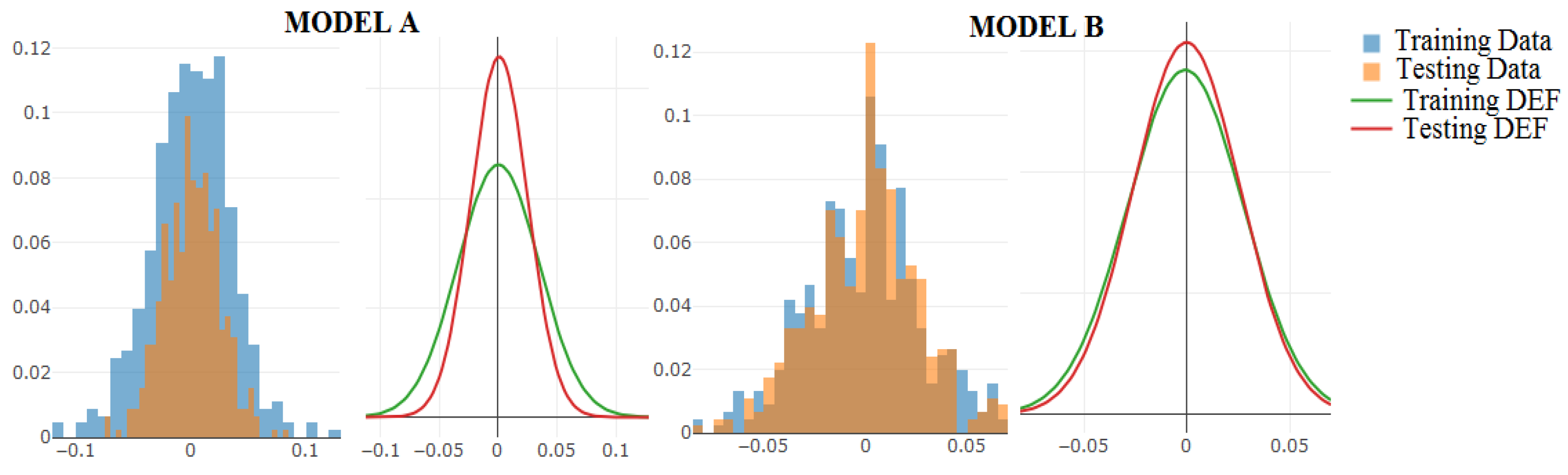
The most important part in error validation is the definition of a good performance, which qualifies the architecture of a neural network model. For this approach, the traditional root mean square error comparison was not the only one considered to validate the models [32]. Instead, the error validation for this research is defined by the comparison of error density functions for training and testing evaluations. Error density functions are continuous functions that represent the attained errors for training and testing evaluations by a known function. The Gaussian function is used to represent these density functions. In this way, the training and testing evaluations can be represented by a Gaussian error density function. It is important to note that a Gaussian function is defined by two parameters: mean or expectation and standard deviation. For this approach, the expectation value is zero and the entire range of errors in the validation is defined by +/− 3 standard deviations by its definition. Under this premise, a certain trained model will present a certain Gaussian density function. For such an attained model, a good performance should be defined by a testing Gaussian density function that is similar to the reached model in the training stage. For instance, Figure 3 shows two models (model A and model B) that evaluate different architectures for the feed rate model as an example. Model A shows a testing evaluation with a particular density function, which is different to the one reached in the training evaluation. In contrast, model B shows a testing error density performance that is quite similar to the one reached in the training evaluations. Table 3 numerically shows the same concept shown in Figure 3. Table 3 also shows additional error comparisons, including the root mean square error (RMSE), median absolute deviation (MAD), maximum and minimum error values, etc. It is important to note that the large differences between RMSE and MAD are indicative of the error density function [30].
To achieve the best model for feed rate and cutting velocity, the following strategy was implemented to validate any possible architecture:
- Consider random architectures with one and two hidden layers with different neurons per layer.
- For each architecture, the training and testing error density functions are obtained. Hereinafter, these Gaussian functions are referred as
- For each architecture, a Euclidean distance is evaluated between the functions of and . This Euclidean distance is calculated with the properties described in Table 3. Equation (3) shows the implementation of this Euclidean distance:
- For each architecture, the maximum distance between the mean error values is considered to be zero. Equation (4) shows the implementation of this distance as the maximum absolute value of the mean property in testing and training error functions:
- A maximum range of error functions must be calculated. This range is defined by the maximum and minimum properties for each error function (, ).
- To consider the skew property for and , the distance between RMSE to MAD is calculated. Equation (6) shows the implementation of this distance as the maximum absolute value for the difference between RMSE and MAD for both and :
- After this, the performance of a suggested model is given by Equation (7), which evaluates the Euclidean distance, mean distance to zero, the total error range and skew distance as a function of and . The constant k allows the function to be adjusted to a certain range of values, which is shown as follows:
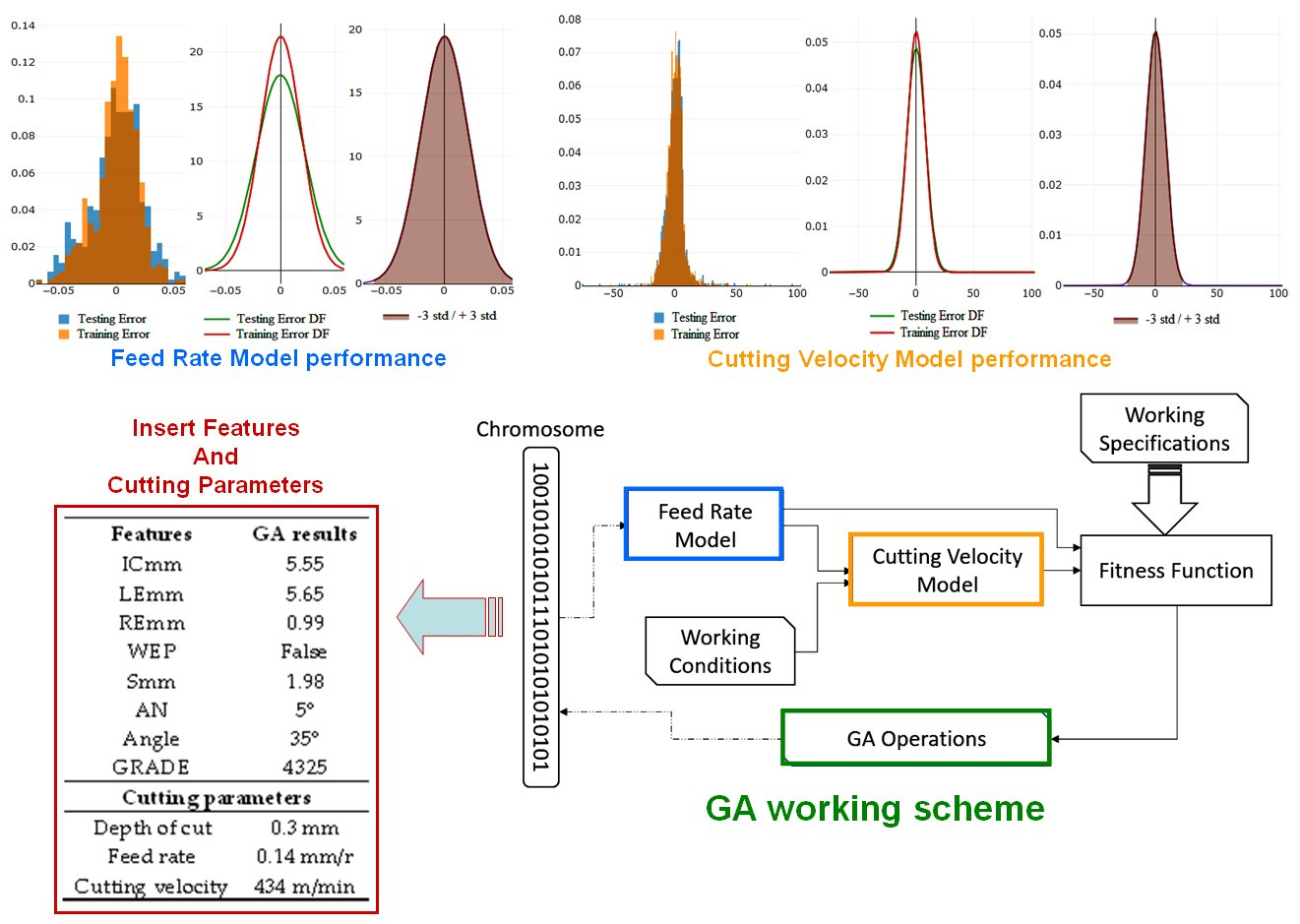
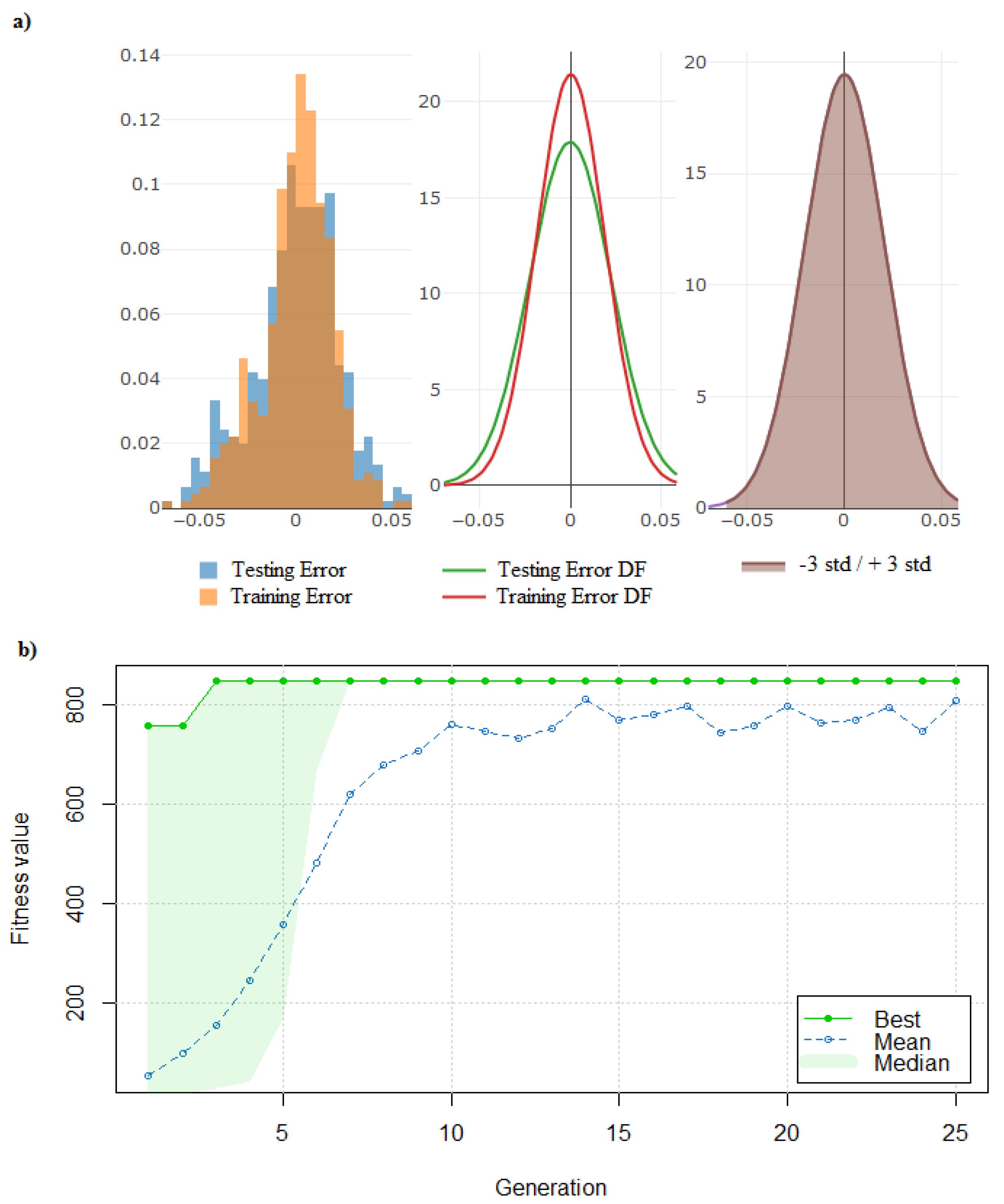
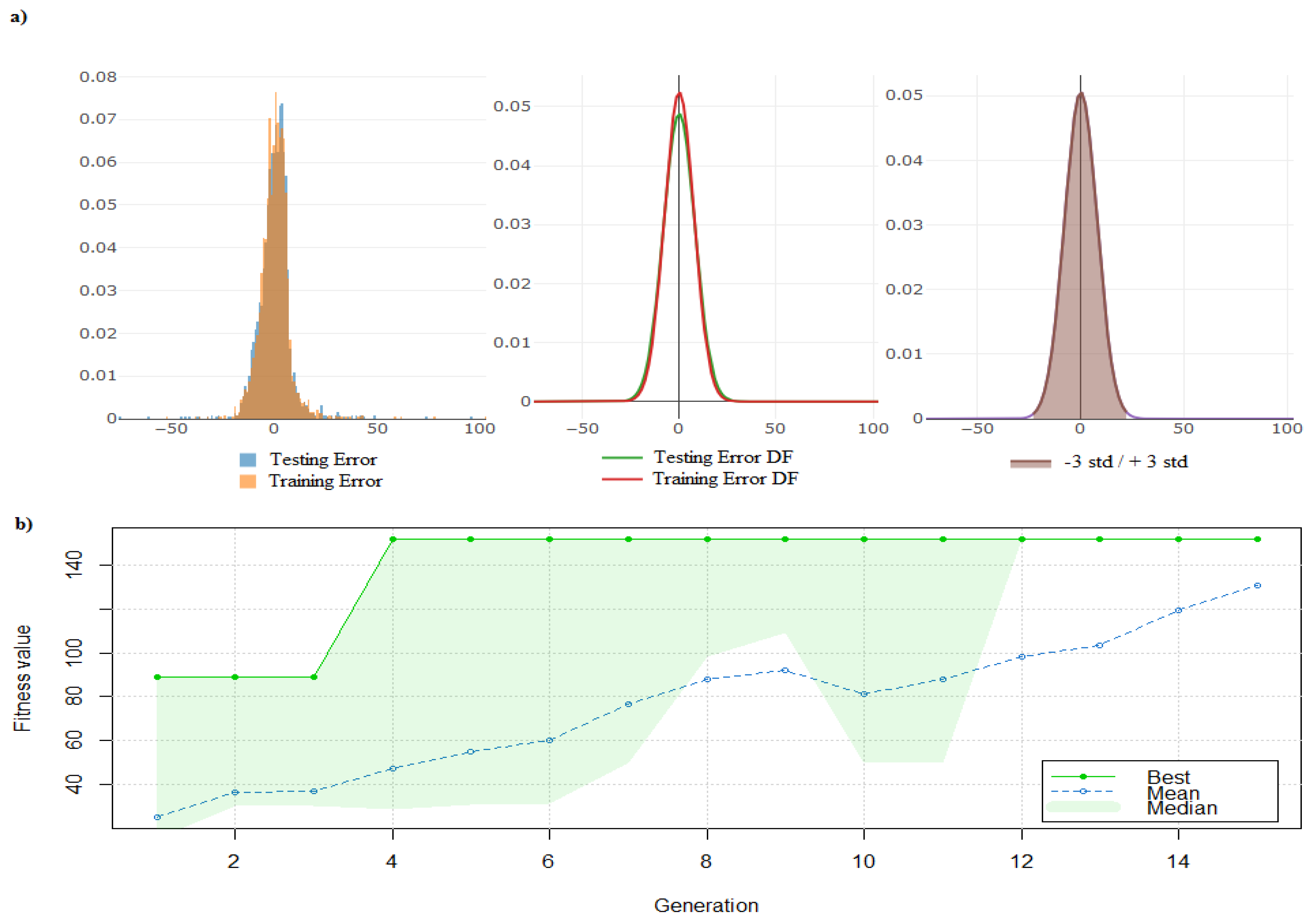
To validate several random architectures, a heuristic optimization search was implemented by using a genetic algorithm for the feed rate and cutting velocity models. The architectures differ from each other in layer and neuron numbers. Furthermore, this genetic algorithm is defined by Equation (7) as the fitness function. Table 4 shows the reached architectures for the feed rate and cutting velocity models. For the feed rate, a neural network model was established with two hidden layers. Furthermore, this model has 15 and 4 neurons per layer. The cutting velocity model was also established with two hidden layers, which has 25 and 7 neurons per layer. The graphical performance for both models is shown in Figure 4 and Figure 5 (feed rate and cutting velocity, respectively). In these figures, it is possible to appreciate the error density function in training and testing evaluations. These figures also show the reached genetic algorithm performance used to converge both models. It is important to note that the optimization by the genetic algorithm allows the achievement of good performance for both models in fewer iterations.
4. Genetic Algorithm Optimization
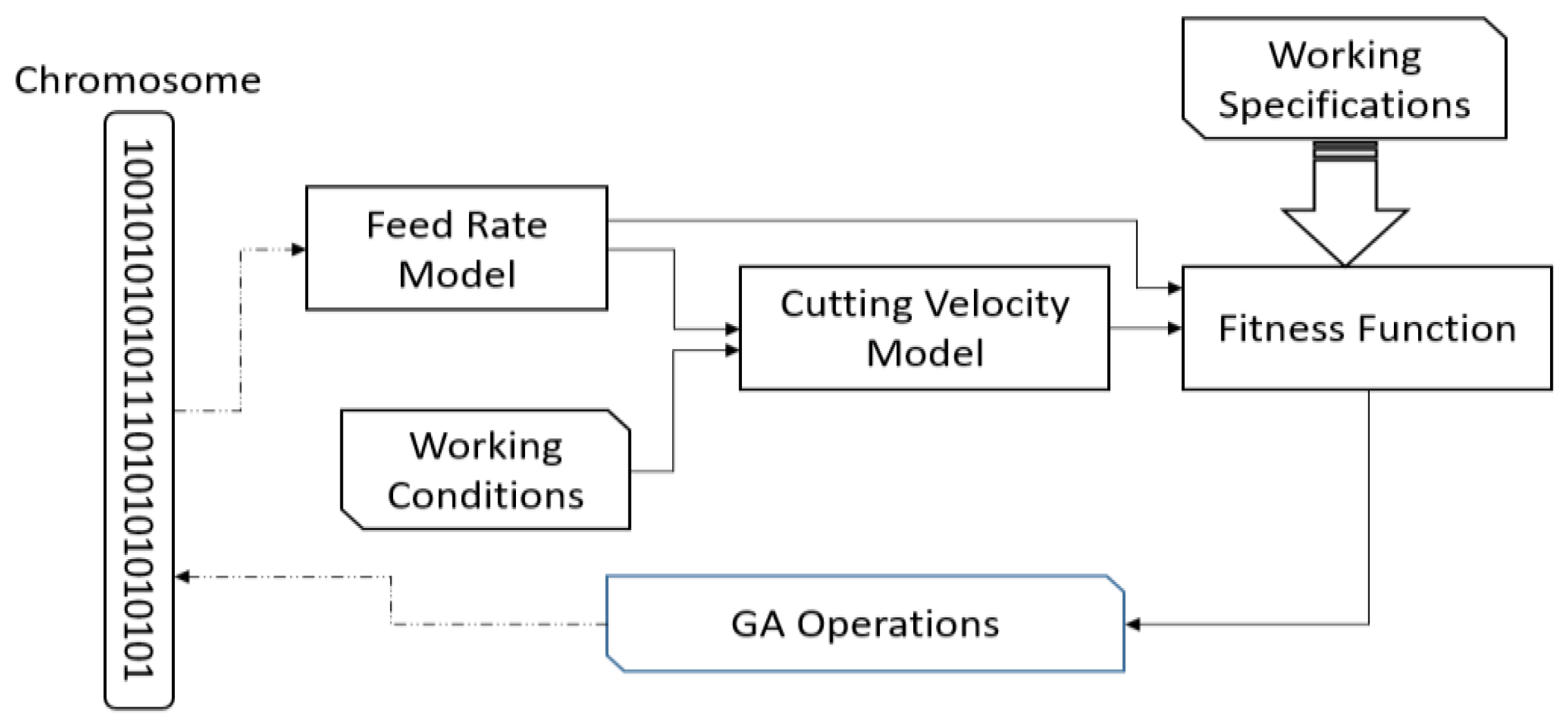
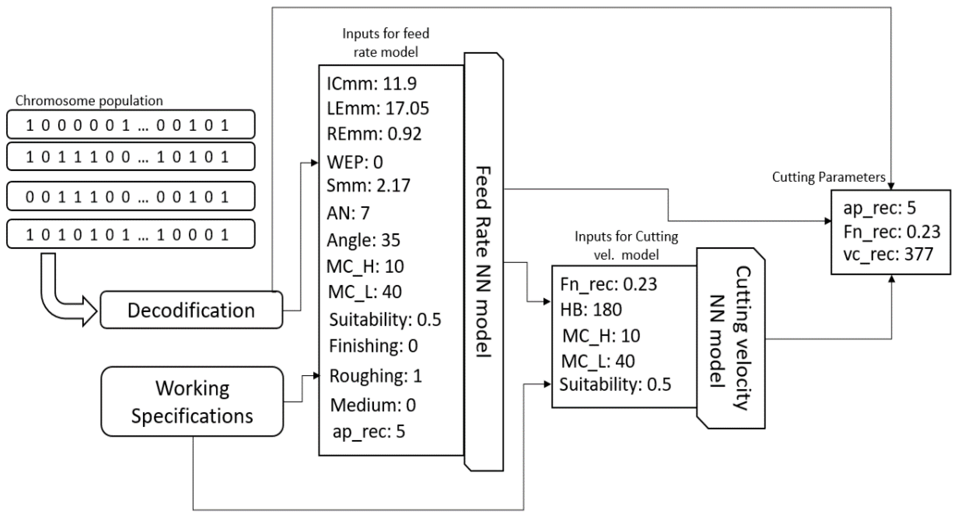
A genetic algorithm (GA) is a heuristic search algorithm inspired by evolutionary mechanisms and biological natural selection. This algorithm defines a searching space of solutions and allows us to find individual solutions, which satisfy a certain condition. This condition is usually referred to as the fitness function [33]. This study aims to define a heuristic search based on GA, which allows us to find an optimal insert-tool for certain working specifications. This insert-tool search is governed by a fitness function, which is defined by a combination of the lowest power consumption, the shortest machining time and acceptable surface roughness among others. Figure 6 shows a general scheme of the proposed GA implementation for this research. Initially, it can be appreciated that the feed rate model evaluates the GA chromosome. After this, the feed rate and working conditions can be used as the inputs for the cutting velocity model. The resulting feed rate and cutting velocity are evaluated by the GA fitness function, which assess the current chromosome along with the working specifications. Finally, the GA operations transform the current population to the next generation. According to their characteristics, the individuals in the population improve with each iteration.
4.1. Working Specifications
The working specifications for the GA represent the framework, which defines the optimization problem. For this research, the working specifications consider three groups: material specifications, machine specifications and general specifications. Table 5 introduces these categories for these working specifications. The material specifications represent the conditions related to the working piece, such as the initial and final diameters, the maximum allowed surface roughness and the machining length. The mechanical properties are also added to this group, including material harness and specific cutting forces. On the other hand, the machine specifications represent the relevant information of the CNC machine in a turning operation. For this approach, the total power available and the maximum spindle speed are considered. The general specifications define additional specifications, which also define a turning operation. For instance, the machine operation is considered in this group of specifications. This specification defines the CTPT feature, which sets the algorithm and considers if the insert-tool solution should be for finishing, medium or roughing operations. Furthermore, a stability parameter is also added to this group of specifications. This stability feature is related to the suitability for the expected insert-tool solution. Finally, the tool life and threshold distances are defined as turning constants, which allow for an adjustment of the accuracy of the algorithm.
4.2. Encode-Decode Chromosomes
A binary chromosome refers to a string of zeros and ones, such as a binary number, and represents a certain bunch of features. Table 1 shows the description of the features of the chromosome structure. On the other hand, each feature has its own encoding length that allows it to be represented in the chromosome string. Table 6 shows the features used to build the GA chromosome and their binary length.
The length properties in Table 6 represent the lengths of the binary numbers used to define each feature. Furthermore, for the described numeric features, there is a specific decoding procedure called linear transformation, which is represented by Equation (8). For this equation, the binary number is evaluated by the function int(Xbinary), which returns the integer value for a binary number. This integer value is then mapped by the maximum, minimum and length values to decode the corresponding features.
The logical features described in Table 6 are represented by one digit with only two possible values (1 or 0 and 5 or 7 for WEP and AN features, respectively). The stability feature has decoding and encoding procedures that differ from the rest of features. The stability feature refers to the suitability feature of an insert-tool. This feature can be set as Excellent, Good or Poor. This parameter is already given by the working specification described in Table 5. However, this information restricts the GA searching space because the grade of an insert-tool is defined under a certain range of application areas. This means that there is only a defined number of grades for a defined stability feature. Table 7 shows the stability condition associated with the insert-tool grades in the present dataset. Under this premise, a grades list (indexed list) and a binary number define the proposed encoding procedure for the features’ stability. The binary number indexes the position for each grade on such list. For instance, we considered the stability “Good” described in Table 8. Since there are only four possible grades in this condition, the binary number to encode this feature is a string of three digits (000, 001, 010, 011, 111, etc.). Thus, the number of ones in such binary number represents the index in the grade list. For two ones in the binary number, the grade is 4225 and for 0 ones in the binary number, the grade is 1125, etc.
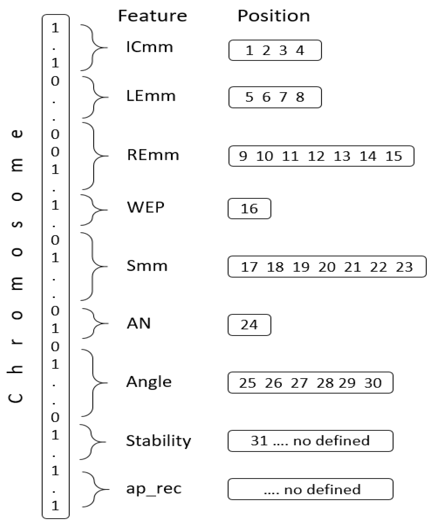
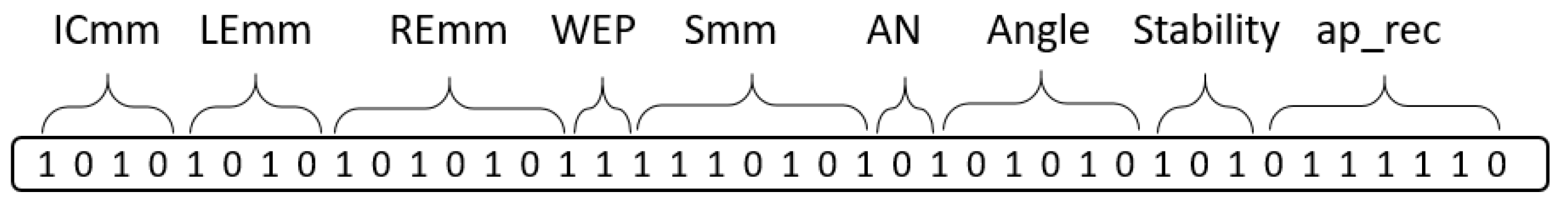
The ap_rec cutting parameter is a special feature for the chromosome definition. The range of this parameter was defined previously as an input to the model. This range is customized by the total and minimum depth of cut values for a certain turning process. Such values are defined with respect to operation issues and specific requirements. The chromosome structure for the GA optimization is shown in Figure 7. This structure defines at least 30 defined positions. It is important to note that each feature has its binary position and length in the chromosome structure.
4.3. Fitness Function Definition
The fitness function is the main concern for the development of the GA and its definition establishes the expected output of the algorithm. For this research, this function was defined as a function that evaluates the lowest power consumption, the shortest machining time and an acceptable surface roughness among others. Equation (9) defines the fitness function for this genetic algorithm optimization. This equation is a summation of goal functions gi, which evaluate power consumption, machining time, surface roughness, etc. Furthermore, each gi function is weighted by a constant ωi, which allows the adjustment of the importance of each gi function.
The goal function, g1, described in Equation (10), evaluates the power consumption ratio in the turning process. This function uses Equation (11) to evaluate the theoretical power consumption, P [20]. Furthermore, the Pnet constant is the total available power in the machine (introduced in Table 5). The constant γ allows for the consideration of the friction losses in the transmission motor [20] although this constant is equal to 1 for this research. Equation (12) shows the cutting force, Fc, as a function of the specific cutting force, Kc, related to the working material, depth of cut (ap_rec) and feed rate (fn_rec) [25]. It is important to note that the specific cutting force, Kc, is a parameter that was also introduced in Table 5.
The goal function, g2, described in Equation (13), defines the machining time ratio, which relates the tool life to the machining time. The tool life, Tlife, is a tool supplier parameter, which defines the approximate tool life for a tool-insert. The machining time is an objective variable evaluated in Equation (14). This defines the machining time in the turning process with a certain group of cutting parameters. Equation (15) presents the spindle speed, n, as a function of the cutting velocity, vc and the current machining diameter, D. It is important to note that n varies according to D. Thus, for each machining pass (diameter decreasing), the spindle speed increases.
The goal function, g3, defined in Equation (16), relates the maximum surface roughness, Ra_max, to the theoretically reached surface roughness, Ra. The parameter Ra_max is a working specification of material that defines the maximum allowed roughness. Ra is an objective variable defined in Equation (17), which estimates the surface roughness for a certain finishing operation [20].
The goal function, g4, defined in Equation (18), relates the objective variable, deuclidean, to the parameter Thd (threshold distance). The variable deuclidean is obtained by Equation (19). This equation calculates the Euclidean distance between the features xi and yi, which are defined by the suggested GA tool-insert features and the nth tool-insert in the dataset, respectively.
The goal function, g5, shown in Equation (20), evaluates the spindle speed ratio, which is used in the turning process. This objective function relates the maximum spindle speed of the machine to the theoretical spindle speed reached in the turning process.
The goal function, g6, shown in Equation (21), evaluates the suitability range for a certain insert grade. This function assesses if a suggested grade is more appropriate for a specific application area compared to other solutions. Grades that are more specific are preferred instead of the general grades.
Overall, there are two fitness functions regarding the turning processes: the finishing or roughing operations. In fact, for the roughing operation, the surface roughness is not considered in the fitness function, but the power consumption, machining time, Euclidean distance, spindle speed ratio and suitability are considered. For the finishing process, the fitness function considers the surface roughness, Euclidean distance and suitability grade. Equations (22) and (23) show the proposed fitness function for the roughing and finishing operations.
4.4. Boundary Constraints
The boundary constraints for the GA optimization define the searching space for the algorithm. These boundary constraints allow us to control the chromosome evolution and ensure that the algorithm is converging towards a suitable solution. The first mechanism for controlling the population evolution is called the feasible solution control. This boundary control prevents infeasible individuals from appearing in the population [20]. This mechanism evaluates the goal function, g4, by the constraint mentioned in Equation (24). Thus, only similar insert-tools are chosen as part of the population. The infeasible solutions are not considered.
Some boundary constraints are established to prevent solutions that evaluate a parameter outside of the machine capabilities. For example, the expression mentioned in Equation (25) avoids GA individuals when evaluating power consumption, which exceeds the maximum power of the machine. The constraint mentioned in Equation (26) avoids solutions that need spindle speeds greater than the maximum defined speed for the machine.
5. Application Examples
This section aims to explain some applications for the algorithm described in this research. Three application examples are used to show the performance and results of the proposed approach. These examples are defined under different working conditions and fitness functions.
5.1. Light Roughing Operation
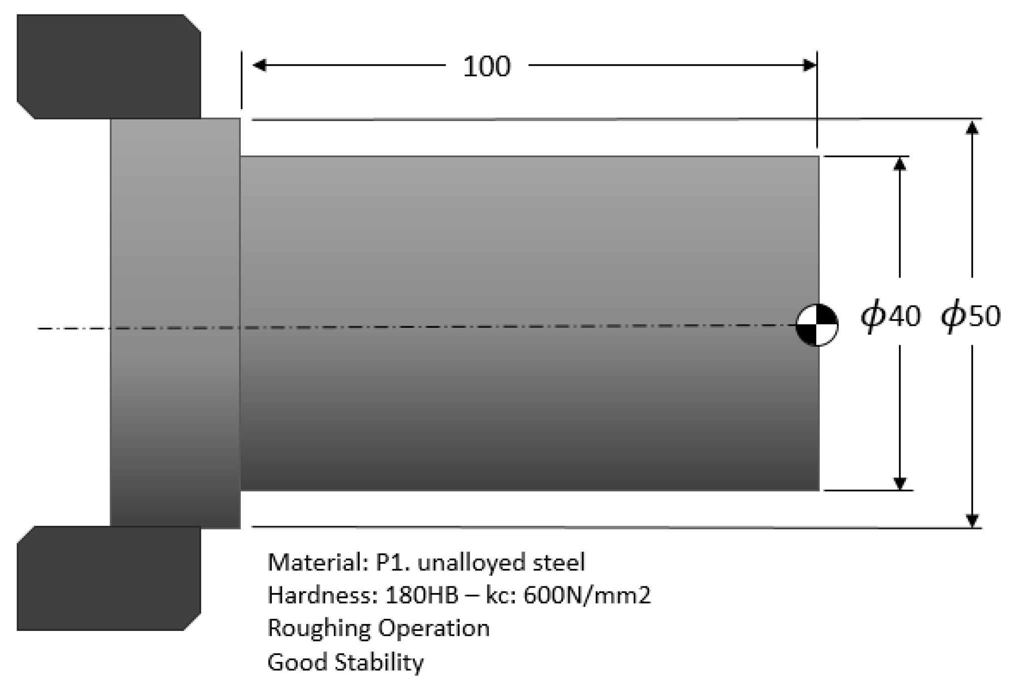
A light roughing machining application can be defined as a turning operation with a small turning depth. In fact, these turning operations could be machined with only one pass. The described algorithm allows us to find a tool-insert solution that balances both power consumption and the number of passes. On the other hand, the machining time does not have the same importance as the power consumption as the number of passes is low. Table 9 introduces the working specifications for this light roughing operation. It sets an initial and a final diameter of 50 mm and 40 mm, respectively. This means a total depth of cut of 5 mm. Additionally, the total machining length is set to 100 mm. Figure 8 illustrates this information. The workpiece material is an unalloyed steel of 180 HB. This material has a specific cutting force of 600 N/mm2. The machine specifications define a small lathe with a power capacity of 10 kW and a maximum spindle speed of 3000 rpm. Equation (27) shows the fitness function for this operation. The power consumption has been weighted to 100 times while the machining time was set to 0.5. This fitness function considers that the impact of power consumption is greater than that of the machining time during the turning process.
Figure 9 provides a complete description of the GA optimization. It begins with the definition of the working specifications, which are presented in Table 9. These specifications set the framework for this example. It is important to note that the working specifications are related to the GA model with respect to some stages ahead, such as the random population, feasible solution control, feed rate and cutting velocity models, boundary constraints and fitness evaluation stages. The stability condition establishes some insert grades as possible solutions since this specification was set at “Good” in Table 9. Such grade solutions were already shown in Table 8, which indexes the list for good stability. With the stability features already defined, the total chromosome length is defined as 40 for this application. On the other hand, the insert features and working specifications form the chromosome structure. Figure 10 describes the chromosome structure for this application. Given the random nature of the GA model, some infeasible individuals can be part of the population. The feasible solution control prevents infeasible solutions from being part of the GA population. The implementation of this control is introduced in Equation (24). This control evaluates a Euclidean distance by adjusting the Thd parameter. All individuals out of the range of distance are discarded from the GA population.
Figure 11 shows the flowchart for obtaining the cutting parameters when given an individual chromosome in the population. It is important to note that some working specifications are used for both the feed rate and cutting velocity neural network models. In addition, the ap_rec cutting parameter (depth of cut) is defined by the GA chromosome and it is used in the feed rate model as an input. Once the cutting parameters, which are namely ap_rec, fn_rec and vc_rec, are obtained, it is possible to evaluate the performance of the current chromosome. Equation (27) shows the proposed fitness function to evaluate the performance of each GA individual. The variables, P, Tm, deuclideanm and n define the power consumption, machining time, Euclidean distance and spindle speed, respectively.
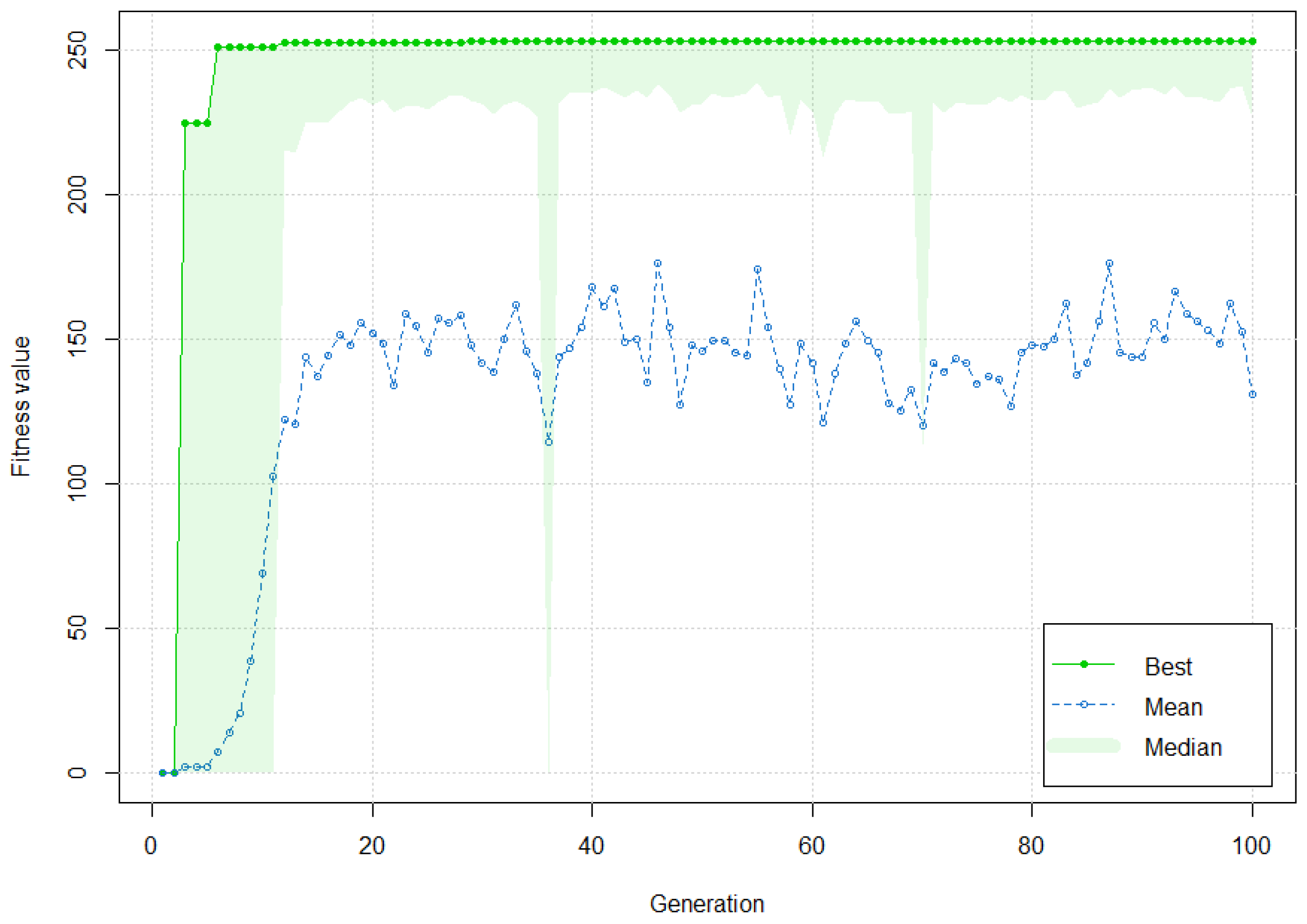
Consistent with the flowchart for GA implementations, the boundary constraints establish population control again, which avoids individual GAs when evaluating parameters beyond the capabilities of the CNC machine. These constraints are related to the total power available and the maximum speed spindle defined in the CNC specifications. Once the entire population has been qualified by the fitness function, the GA operation crosses, selects and mutates the chromosomes to evolve them toward the next generation. In this way, after a certain number of iterations, the population is evolved enough towards a suitable insert-tool solution with its cutting parameters, as shown in Figure 12. Table 10 shows the reached non-existent insert by the GA evolution next to the defined closer tool-insert in the dataset. The reached tool-insert and its cutting parameters are presented as well. In Table 11, the evaluation for the goal variables, which define the performance for the suggested tool-insert, is introduced.
5.2. Heavy Roughing Operation
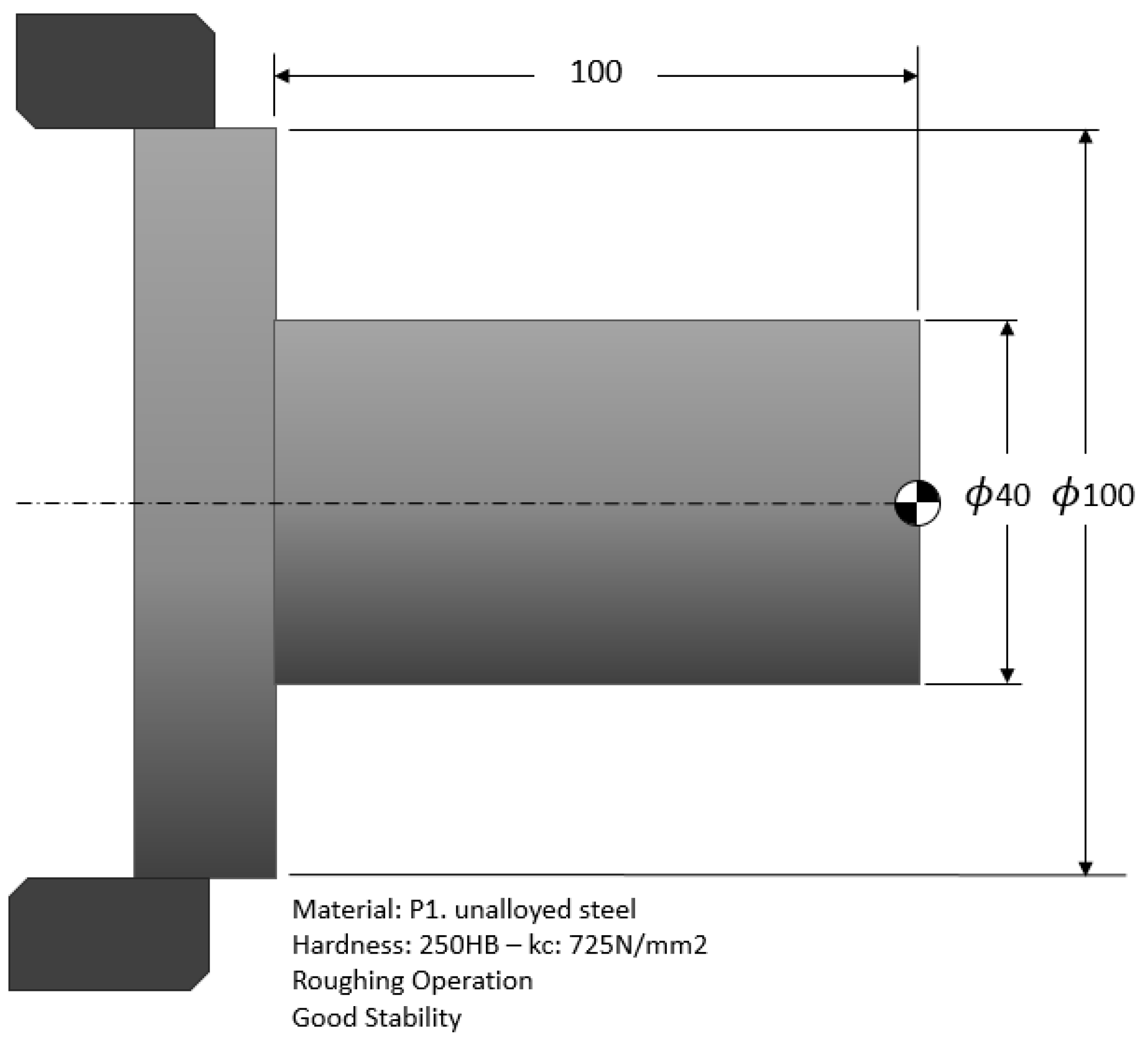
A heavy roughing application can be defined as a turning operation with a large depth turning. These turning operations cannot be machined in a single pass unlike light roughing machining. For this reason, the fitness function for these turning operations considers the machining time evaluation more than the power consumption. Table 12 introduces the working specifications for this roughing operation. It sets an initial diameter and a final diameter to 100 mm and 40 mm, respectively, which defines a total depth turning of 30 mm. Additionally, the total machining length is set to 100 mm. The geometrical information for this example is presented in Figure 13. The workpiece material is an unalloyed steel of 250 HB with a specific cutting force of 725 N/mm2. Moreover, for this operation, the stability condition is set to “Good.” The machine specifications define a small lathe with a total power capability of 10 kW and a maximum spindle speed of 3000 rpm. Equation (28) shows the fitness function for this operation. The machining time has been weighted 10 times, while the power consumption has been weighted 0.5 times. In this way, the fitness function establishes that the solution must prioritize the machining time instead of the power consumption.
Table 13 shows the results for the GA evolution, which are the obtained features for the GA algorithm next to the closer tool-insert in the dataset. This table also presents the suggested tool-insert and its cutting parameters for this operation. Furthermore, in Table 14, the evaluation for the goal variables, which define the performance for the reached tool-insert, is introduced.
5.3. Finishing Operation
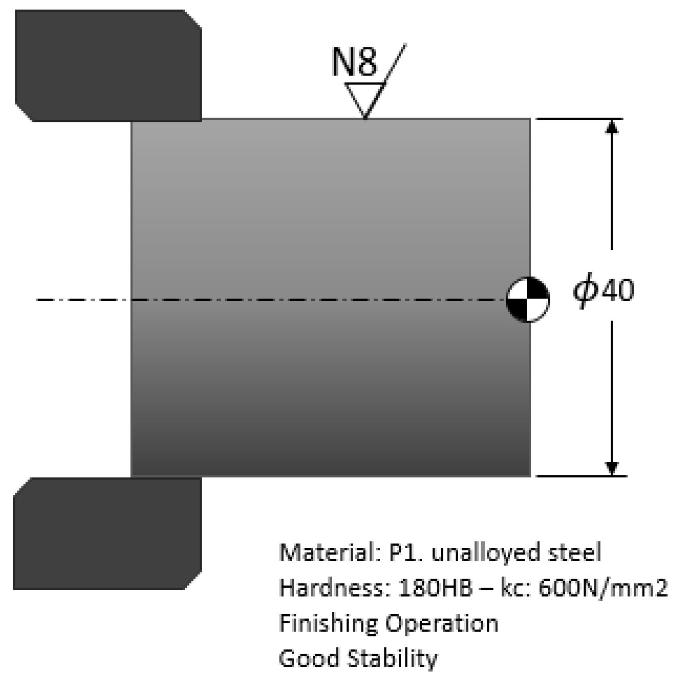
Finishing operations differ from roughing operations mainly with regards to the fitness function. In this operation, the stability and surface roughness performance define the tool-insert solution. The stability features must be defined in such a way that the selected grade belongs to the lower ISO area application, which is related to the wear resistance performance. This area application is specified for finishing operations. Furthermore, the surface roughness performance must be lower than the maximum roughness defined by the working specifications of the process. Table 15 introduces the working specifications of this finishing operation. It sets a final diameter of 40 mm and a maximum surface roughness of ISO N8. This surface specification defines a roughness of 3 μm. The geometrical information for this example is presented in Figure 14. The workpiece material is an unalloyed steel of 180 HB with a specific cutting force of 600 N/mm2. For this operation, the stability condition is set to “Good.” The machine specifications define a medium lathe with a total power of 15 kW and a maximum spindle speed of 6000 rpm. Equation (29) sets the fitness function for this operation. This function evaluates the goal functions related to surface roughness and stability grade.
Table 16 shows the results for the GA evolution, which are the obtained features of the GA algorithm next to the closer tool-insert in the dataset. The information related to the suggested tool-insert is also presented. The reached tool was VBMT 11 03 12-PF 4325. Table 17 introduces the evaluation for the goal variables, which define the performance of the suggested tool-insert.
6. Conclusions
Neural network models for the selection of cutting inserts and cutting parameters were designed. These models were applied to roughing and finishing operations. This research uses the information from a tool supplier to embed knowledge for the tool-insert selection and optimization system developed in this research. The proposed system is based on artificial neural networks (ANNs) and a genetic algorithm (GA). These represent the modeling and optimization part of this research, respectively. For the modeling, two ANNs were implemented. These ANNs are able to infer the feed rate and cutting velocity parameters. The feed rate model is defined as a function of insert features and a set depth of the cut. The insert features represent the macro-geometries of a tool-insert, which include the cutting length, thickness, nose angle, nose radius, size and grade among others. For the cutting velocity model, the inputs are the material specifications and a set feed rate. The material specifications are defined as inherent features of a working material for turning processes. They include hardness, specific cutting force and ISO material group.
For the neural network validation, an error comparison based on density functions was implemented. This approach proposed an alternative solution for the error validation of regression models based on the recommended data by a supplier. To evaluate some architectures of the ANN models, a heuristic search based on GA was used. This approach evaluated the possible architectures and evolved them toward the most feasible one. For the proposed research, a heuristic searching method for a feasible tool-insert based on its characteristics in a certain environment was also introduced. The algorithm used for this search was a GA. The introduced GA optimization searches for an optimal tool-insert, which adapts to a working specification and evaluates an acceptable performance given by a customized objective function. This objective function evaluates the performance under certain working conditions, such as the lowest power consumption, the shortest machining time and an acceptable surface roughness. In this present study, different goal functions referring to different force models or tool life models can be used when designing the fitness function in order to obtain the optimal tool-insert with specific considerations. This research presents a model to simulate knowledge and expertise, which embeds the information from a tool supplier. It returns the most suitable insert-tool as a result, given certain working conditions. This research did not use a lookup table approach in the database as it instead modeled the mechanical relations between the geometrical features of an insert-tool and its recommended cutting parameters. This tool-insert selection and optimization system can embed the data from other models, different tool suppliers, previous machining works and expertise from machine-shop workers. However, because of the inherent discrepancy among different datasets, additional factors, such as input variation and data types, must be considered when using the developed system and approaches. Furthermore, because the developed system successfully represents the complex relationship between the working condition and the cutting parameters, the developed system can be a plug-in for CAD/CAM software or can be integrated with the controller of a CNC machine tool to be an auxiliary function for the automatic selection of the cutting parameters based on the preset working conditions presented in the part program. For this research, a fully connected ANN model was used due to the representation of a multi-dimensional space using the training data obtained from a database. Other networks with diverse characteristics, such as the convolutional networks, could also be used in future researches. Moreover, methods, such as the support vector machine and probabilistic regression, could be used for regression modeling. This research has used a GA for optimization. However, methods, such as the particle swarm optimization and gradient descent technique, can also be used to carry out optimization.
Author Contributions
Investigation, B.S.-P., D.H. and S.-S.Y.; Supervision, S.-S.Y.
Funding
This research was funded in part by the Ministry of Science and Technology, Taiwan, R.O.C., under Contract MOST104-2221-E-027-132 and MOST103-2218-E-009-027-MY2.
Acknowledgments
The authors would like to thank Hao-Wei Nien (Advantech-LNC Technology Co. Ltd., Taiwan, R.O.C.) and Chao-Choung Mai (ITRI Intelligent Machinery Technology Center, Taiwan, R.O.C.) for their suggestions.
Conflicts of Interest
The authors declare no conflict of interest.
References
- Weyer, S.; Schmitt, M.; Ohmer, M.; Gorecky, D. Towards industry 4.0—Standardization as the crucial challenge for highly modular, multi-vendor production systems. IFAC-Pap. 2015, 48, 579–584. [Google Scholar] [CrossRef]
- Leo Kumar, S.P. State of the art—Intense review on artificial intelligence systems application in process planning and manufacturing. Eng. Appl. Artif. Intell. 2017, 65, 294–329. [Google Scholar] [CrossRef]
- Zarkti, H.; El Mesbahi, A.; Rechia, A.; Jaider, O. Towards an automatic-Optimized tool selection for milling process, based on data from Sandvik Coromant. In Proceedings of the Xème Conférence Internationale: Conception et Production Intégrées, Tanger, Morocco, 3–4 December 2015. [Google Scholar]
- Arrazola, P.J.; Özel, T.; Umbrello, D.; Davies, M.; Jawahir, I.S. Recent advances in modelling of metal machining processes. CIRP Ann. 2013, 62, 695–718. [Google Scholar] [CrossRef]
- Ganesh, N.; Kumar, M.U.; Kumar, C.V.; Kumar, B.S. Optimization of cutting parameters in turning of EN 8 steel using response surface method and genetic algorithm. Int. J. Mech. Eng. Robot. Res. 2014, 3, 75–86. [Google Scholar]
- Yang, Y.; Li, X.; Gao, L.; Shao, X. A new approach for predicting and collaborative evaluating the cutting force in face milling based on gene expression programming. J. Netw. Comput. Appl. 2013, 36, 1540–1550. [Google Scholar] [CrossRef]
- Cabrera, F.M.; Beamud, E.; Hanafi, I.; Khamlichi, A.; Jabbouri, A. Fuzzy logic-based modeling of surface roughness parameters for CNC turning of PEEK CF30 by TiN-coated cutting tools. J. Thermoplast. Compos. Mater. 2011, 24, 399–413. [Google Scholar] [CrossRef]
- Joshi, S.R.; Ganjigatti, J.P. Application of general regression neural networks for forward and reverse modeling of aluminum alloy AA5083; H111 TIG welding process and comparison with feed forward back propagation, Elman back propagation neural networks. Int. J. Eng. Technol. Sci. Res. 2017, 4, 16–26. [Google Scholar]
- Li, H.Z.; Guo, S.; Li, C.J.; Sun, J.Q. A hybrid annual power load forecasting model based on generalized regression neural network with fruit fly optimization algorithm. Knowl. -Based Syst. 2013, 37, 378–387. [Google Scholar] [CrossRef]
- Cairns, J.; McPherson, N.; Galloway, A. Using artificial neural networks to identify and optimise the key parameters affecting geometry of a GMAW fillet weld. In Proceedings of the 18th International Conference on Joining Materials, JOM-18, Helsingor, Denmark, 26–29 April 2015. [Google Scholar]
- Arezoo, B.; Ridgway, K.; Al-Ahmari, A.M.A. Selection of cutting tools and conditions of machining operations using an expert system. Comput. Ind. 2000, 42, 43–58. [Google Scholar] [CrossRef]
- Dereli, T.; Filiz, I.H.; Baykasoglu, A. Optimizing cutting parameters in process planning of prismatic parts by using genetic algorithms. Int. J. Prod. Res. 2001, 39, 3303–3328. [Google Scholar] [CrossRef]
- Benkedjouh, T.; Medjaher, K.; Zerhouni, N.; Rechak, S. Health assessment and life prediction of cutting tools based on support vector regression. J. Intell. Manuf. 2015, 26, 213–223. [Google Scholar] [CrossRef]
- Özel, T.; Hsu, T.K.; Zeren, E. Effects of cutting edge geometry, workpiece hardness, feed rate and cutting speed on surface roughness and forces in finish turning of hardened AISI H13 steel. Int. J. Adv. Manuf. Technol. 2004, 25, 262–269. [Google Scholar] [CrossRef]
- Xiong, J.; Zhang, G.; Hu, J.; Wu, L. Bead geometry prediction for robotic GMAW-based rapid manufacturing through a neural network and a second-order regression analysis. J. Intell. Manuf. 2012, 25, 157–163. [Google Scholar] [CrossRef]
- Babu, K.V.; Narayanan, R.G.; Kumar, G.S. An expert system based on artificial neural network for predicting the tensile behavior of tailor welded blanks. Expert Syst. Appl. 2009, 36, 10683–10695. [Google Scholar] [CrossRef]
- Özel, T.; Karpat, Y. Predictive modeling of surface roughness and tool wear in hard turning using regression and neural networks. Int. J. Mach. Tools Manuf. 2005, 45, 467–479. [Google Scholar] [CrossRef]
- Malinov, S.; Sha, W.; McKeown, J.J. Modelling the correlation between processing parameters and properties in titanium alloys using artificial neural network. Comput. Mater. Sci. 2001, 21, 375–394. [Google Scholar] [CrossRef] [Green Version]
- Kuo, R.J.; Chen, C.H.; Hwang, Y.C. An intelligent stock trading decision support system through integration of genetic algorithm based fuzzy neural network and artificial neural network. Fuzzy Sets Syst. 2001, 118, 21–45. [Google Scholar] [CrossRef]
- Quiza Sardiñas, R.; Rivas Santana, M.; Alfonso Brindis, E. Genetic algorithm-based multi-objective optimization of cutting parameters in turning processes. Eng. Appl. Artif. Intell. 2006, 19, 127–133. [Google Scholar] [CrossRef]
- Cus, F.; Balic, J. Optimization of cutting process by GA approach. Robot. Comput. -Integr. Manuf. 2003, 19, 113–121. [Google Scholar] [CrossRef]
- Suresh, P.V.S.; Rao, P.V.; Deshmukh, S.G. A genetic algorithmic approach for optimization of surface roughness prediction model. Int. J. Mach. Tools Manuf. 2002, 42, 675–680. [Google Scholar] [CrossRef]
- Yang, W.H.; Tarng, Y.S. Design optimization of cutting parameters for turning operations based on the Taguchi method. J. Mater. Process. Technol. 1998, 84, 122–129. [Google Scholar] [CrossRef]
- Thamizhmanii, S.; Saparudin, S.; Hasan, S. Analyses of surface roughness by turning process using Taguchi method. J. Achiev. Mater. Manuf. Eng. 2007, 20, 503–506. [Google Scholar]
- Sandvik Coromant. Available online: https://www.sandvik.coromant.com/en-gb/pages/default.aspx (accessed on 9 October 2017).
- Murata, N.; Yoshizawa, S.; Amari, S. Network information criterion-determining the number of hidden units for an artificial neural network model. IEEE Trans. Neural Netw. 1994, 5, 865–872. [Google Scholar] [CrossRef] [PubMed] [Green Version]
- Arnaiz-González, Á.; Fernández-Valdivielso, A.; Bustillo, A.; López de Lacalle, L.N. Using artificial neural networks for the prediction of dimensional error on inclined surfaces manufactured by ball-end milling. Int. J. Adv. Manuf. Technol. 2016, 83, 847–859. [Google Scholar] [CrossRef]
- Jain, S.P.; Ravindra, H.V.; Ugrasen, G.; Prakash, G.V.N.; Rammohan, Y.S. Study of surface roughness and AE signals while machining titanium grade-2 material using ANN in WEDM. In Materials Today: Proceedings; Elsevier: Amsterdam, The Netherlands, 2017; pp. 9557–9560. [Google Scholar]
- Anastasiadis, A.D.; Magoulas, G.D.; Vrahatis, M.N. New globally convergent training scheme based on the resilient propagation algorithm. Neurocomputing 2005, 64, 253–270. [Google Scholar] [CrossRef]
- Twomey, J.M.; Smith, A.E. Validation and verification. In Artificial Neural Networks for Civil Engineers: Fundamentals and Applications; Expert Systems and Artificial Intelligence Committee, Ed.; American Society of Civil Engineers: Reston, VA, USA, 1997; pp. 44–64. [Google Scholar]
- Olden, J.D.; Jackson, D.A. Illuminating the “black box”: A randomization approach for understanding variable contributions in artificial neural networks. Ecol. Model. 2002, 154, 135–150. [Google Scholar] [CrossRef]
- Bishop, C.M. Pattern Recognition and Machine Learning; Springer: New York, NY, USA, 2011. [Google Scholar]
- Scrucca, L. GA: A package for genetic algorithms in R. J. Stat. Softw. 2013, 53, 1–37. [Google Scholar] [CrossRef]
Figure 1.
Tool-insert features considered in this study [25]; cutting length (LEmm); corner radius (REmm); thickness (Smm); and shape angle (SC).
Figure 1.
Tool-insert features considered in this study [25]; cutting length (LEmm); corner radius (REmm); thickness (Smm); and shape angle (SC).

Figure 2.
Cutting velocity, hardness and feed rate scatter.

Figure 3.
Example of error density function comparison.

Figure 4.
Feed rate model performance; (a) Error density function comparison; and (b) Genetic algorithm performance.
Figure 4.
Feed rate model performance; (a) Error density function comparison; and (b) Genetic algorithm performance.

Figure 5.
Cutting velocity model performance; (a) Error density function comparison; (b) Genetic algorithm performance.
Figure 5.
Cutting velocity model performance; (a) Error density function comparison; (b) Genetic algorithm performance.

Figure 6.
GA (genetic algorithm) working scheme.

Figure 7.
Chromosome structure.

Figure 8.
Example of a light roughing operation.

Figure 9.
Flowchart of the GA implementation.

Figure 10.
The GA chromosome structure.

Figure 11.
Neural network models in GA optimization.

Figure 12.
Example of GA performance for light roughing operation.

Figure 13.
Example of heavy roughing operation.

Figure 14.
Example of a finishing operation.


Table 1.
Feed rate dataset–feature descriptions; CTPT: finishing, medium and roughing operations.
| Feature Name | Data Type | Description |
|---|---|---|
| ICmm | Numeric | Inscribed circle |
| AN | Logical | Clarence angle |
| LEmm | Numeric | Cutting length |
| REmm | Numeric | Nose radius |
| Smm | Numeric | Thickness |
| SC | Numeric | Insert shape angle |
| Finishing | Logical | CTPT finishing operation |
| Medium | Logical | CTPT medium operation |
| Roughing | Logical | CTPT roughing operation |
| WEP | Logical | Wiper property |
| MC_L | Numeric | Low machine condition |
| MC_H | Numeric | High machine condition |
| MC_Suitability | Numeric | Suitability machine condition |
| ap_rec | Numeric | Recommended depth of cut |
Table 2.
Cutting velocity dataset–feature descriptions.
| Feature Name | Data Type | Description |
|---|---|---|
| MC_L | Numeric | Low machine condition |
| MC_H | Numeric | High machine condition |
| MC_Suitability | Numeric | Suitability machine condition |
| HB | Numeric | Hardness material |
| fn_rec | Numeric | Recommended feed rate |
Table 3.
Error validation example.
| Properties | Model A | Model B | ||
|---|---|---|---|---|
| Training Data | Testing Data | Training Data | Testing Data | |
| Mean square error | 11.9 × 10⁻⁴ | 5.8 × 10⁻⁴ | 7.8 × 10⁻⁴ | 6.7 × 10⁻⁴ |
| Root mean square error | 34.5 × 10⁻³ | 24.2 × 10⁻³ | 28.0 × 10⁻³ | 25.9 × 10⁻³ |
| Median absolute deviation | 22.4 × 10⁻³ | 16.7 × 10⁻³ | 18.2 × 10⁻³ | 16.7 × 10⁻³ |
| Max. value | 0.1275 | 0.0811 | 0.0698 | 0.0675 |
| Min. value | −0.1167 | −0.0791 | −0.0828 | −0.0828 |
| Mean | 19.4 × 10⁻⁵ | 87.0 × 10⁻⁵ | −8.0 × 10⁻⁴ | −1.8 × 10⁻⁴ |
| Standard deviation | 34.5 × 10⁻³ | 24.2 × 10⁻³ | 28.0 × 10⁻³ | 26.0 × 10⁻³ |
Table 4.
Error validation for feed rate and cutting velocity models.
| Models | Feed Rate | Cutting Velocity | ||
|---|---|---|---|---|
| Datasets | Training | Testing | Training | Testing |
| Architecture | 15–4 | 15–5 | ||
| Mean square error | 4.95 × 10⁻⁴ | 3.45 × 10⁻⁴ | 57.71 | 66.66 |
| Root mean square error | 2.22 × 10⁻² | 1.8 × 10⁻² | 7.59 | 8.16 |
| Median absolute deviation | 1.41 × 10⁻² | 1.10 × 10⁻² | 3.84 | 3.91 |
| Max. value | 5.82 × 10⁻² | 5.82 × 10⁻² | 102.82 | 95.51 |
| Min. value | −6.97 × 10⁻² | −6.71 × 10⁻² | −52.76 | −75.10 |
| Mean | −1.73 × 10⁻⁴ | 1.24 × 10⁻⁴ | −3.60 × 10⁻² | −3.61 × 10⁻² |
| Standard deviation | 2.22 × 10⁻² | 1.86 × 10⁻² | 7.59 | 8.16 |
| dED | 6.55 × 10⁻³ | 25.16 | ||
| dmean | 1.73 × 10⁻³ | 3.61 × 10⁻² | ||
| drange | 1.28 × 10⁻¹ | 170.61 | ||
| dskew | 8.14 × 10⁻³ | 4.25 | ||
| k | 1 × 10⁻⁵ | 1 × 10⁵ | ||
| Fperfo | 845.26 | 151.68 | ||
Table 5.
Working specifications.
| Material specifications | ||
| Initial diameter | Di | Numeric values |
| Final diameter | Df | Numeric values |
| Machining length | Lm | Numeric values |
| Hardness | HB | Numeric values |
| Specific cutting force | Kc | Numeric values |
| Max. surface roughness | Ra_max | Numeric values |
| Machine specifications | ||
| Main motor power | Pnet | Numeric values |
| Max. spindle speed | nmax | Numeric values |
| General specifications | ||
| Machine operation | CTPT | Finishing–Medium–Roughing |
| Stability | / | Excellent–Good–Poor |
| Toot life | Tlife | Numeric values |
| Threshold distance | Thd | Numeric values |
Table 6.
Insert features descriptions for the decoding procedure.
| Name | Type | Range | Length of Binary Numbers |
|---|---|---|---|
| ICmm | Numeric | 15.875–3.970 | 4 |
| LEmm | Numeric | 21.20–5.65 | 4 |
| REmm | Numeric | 1.19–0.02 | 7 |
| WEP | Logical | 1 or 0 | 1 |
| Smm | Numeric | 5.56–1.98 | 7 |
| AN | Logical | 7 or 5 | 1 |
| Angle | Numeric | 90–35 | 6 |
| Stability | Factor | not defined | not defined |
| ap_rec | Numeric | not defined | 7 |
Table 7.
Grade stability.
| GRADE | Suitability | Stability | GRADE | Suitability | Stability |
|---|---|---|---|---|---|
| 1125 | 75% | Good | 4305 | 100% | Excellent |
| 1515 | 75% | Good | 4315 | 83.3% | Excellent |
| 1525 | 100% | Excellent | 4325 | 50% | Good |
| 235 | 0% | Poor | 4335 | 16.6% | Poor |
| 4215 | 83.3% | Excellent | 5015 | 100% | Excellent |
| 4225 | 50% | Good | GC15 | 100% | Excellent |
| 4235 | 20% | Poor | GC30 | 0% | Poor |
Table 8.
Indexed list for good stability.
| Index | Grade | Stability |
|---|---|---|
| 0 | 1125 | Good |
| 1 | 1515 | Good |
| 2 | 4225 | Good |
| 3 | 4325 | Good |
Table 9.
Working specifications of the light roughing operation example.
| Material Specifications | ||
| Initial diameter | Di | 50 mm |
| Final diameter | Df | 40 mm |
| Machining length | Lm | 100 mm |
| Hardness | HB | 180 HB |
| Specific cutting force | Hc | 600 N/mm2 |
| Machine Specifications | ||
| Main motor power | Pnet | 10 kW |
| Maximum spindle speed | nmax | 3000 rpm |
| General Specifications | ||
| Machine operation | CTPT | Roughing |
| Stability | / | Good |
| Toot life | Tlife | 15 min |
| Threshold distance | Thd | 10 |
| Range ap_rec | ap_rec | 0.01 mm–5 mm |
Table 10.
Results of the light roughing operation example.
| Features | GA Results | Closer Insert |
| ICmm | 8.73 | 6.35 |
| LEmm | 10.5 | 10.3 |
| REmm | 0.68 | 0.39 |
| WEP | false | false |
| Smm | 2.37 | 2.38 |
| AN | 7° | 7° |
| Angle | 65° | 60° |
| GRADE | 4325 | 4325 |
| Cutting Parameters | ||
| Closer insert | TCMT 11 02 04-UR 4325 | |
| Depth of cut | 5 mm | |
| Feed rate | 0.288 mm/r | |
| Cutting velocity | 346 m/min | |
Table 11.
Goal variables evaluation for light roughing operation example.
| Goal Variable | Variable | Evaluation |
|---|---|---|
| Power consumption | P | 5 kW |
| Machining time | Tm | 0.34 min |
| Euclidean distance | deuclidean | 6.307 |
| Spindle speed | n | 2761 rpm |
| High machining condition | MC_H | 40 |
| Low machining condition | MC_L | 10 |
| Fitness function | fitness | 225.69 |
Table 12.
Working specifications of the heavy roughing operation example.
| Material Specifications | ||
| Initial diameter | Di | 100 mm |
| Final diameter | Df | 40 mm |
| Machining length | Lm | 100 mm |
| Hardness | HB | 250 HB |
| Specific cutting force | Kc | 725 N/mm2 |
| Machine Specifications | ||
| Main motor power | Pnet | 10 kW |
| Maximum spindle speed | nmax | 3000 rpm |
| General Specifications | ||
| Machine operation | CTPT | Roughing |
| Stability | / | Good |
| Toot life | Tlife | 15 min |
| Threshold distance | Thd | 10 |
| Range ap_rec | ap_rec | 0.01–5 mm |
Table 13.
Results of the heavy roughing operation example.
| Features | GA Results | Closer Insert |
| ICmm | 15.87 | 12.07 |
| LEmm | 21.2 | 11.7 |
| REmm | 0.609 | 1.19 |
| WEP | false | false |
| Smm | 5.56 | 4.76 |
| AN | 7° | 7° |
| Angle | 90° | 90° |
| GRADE | 4325 | 4325 |
| Cutting Parameters | ||
| Closer insert | CCMT 12 04 12-PR 4325 | |
| Number of passes | 6 | |
| Depth of cut | 5 mm | |
| Feed rate | 0.325 mm/r | |
| Cutting velocity | 261 m/min | |
Table 14.
Goal variables evaluation of the heavy roughing operation example.
| Goal variable | Variable | Evaluation |
|---|---|---|
| Power consumption | P | 5.13 kW |
| Total power consumption | 30.83 kW | |
| Machining time | Tm | 1.84 min |
| Euclidean distance | deuclidean | 4.7830 |
| Spindle speed | 2080 rpm | |
| High machining condition | MC_H | 40 |
| Low machining condition | MC_L | 10 |
| Fitness function | Fitness | 86.261 |
Table 15.
Working specifications of the finishing operation example.
| Material Specifications | ||
| Final diameter | Df | 40 mm |
| Machining length | Lm | 50 mm |
| Hardness | HB | 180 HB |
| Specific cutting force | Kc | 600 N/mm2 |
| Max. surface roughness | Ra_max | 3 μm |
| Machine Specifications | ||
| Main motor power | Pnet | 15 kW |
| Maximum spindle speed | nmax | 6000 rpm |
| General Specifications | ||
| Machine operation | CTPT | Finishing |
| Stability | / | Good |
| Toot life | Tlife | 15 min |
| Threshold distance | Thd | 20 |
| Range ap_rec | ap_rec | 0.01–5 mm |
Table 16.
Results of the finishing operation example.
| Features | GA Results | Closer Insert |
| ICmm | 5.55 | 6.35 |
| LEmm | 5.65 | 9.87 |
| REmm | 0.99 | 1.19 |
| WEP | False | false |
| Smm | 1.98 | 3.18 |
| AN | 5° | 5° |
| Angle | 35° | 35° |
| GRADE | 4325 | 4325 |
| Cutting Parameters | ||
| Closer insert | VBMT 11 03 12-PF 4325 | |
| Depth of cut | 0.3 mm | |
| Feed rate | 0.14 mm/r | |
| Cutting velocity | 434 m/min | |
Table 17.
Goal variables evaluation of the finishing operation example.
| Goal Variable | Variable | Evaluation |
|---|---|---|
| Power consumption | P | 0.189 kW |
| Machining time | Tm | 0.343 min |
| Euclidean distance | deuclidean | 6.48 |
| Spindle speed | 3456 rpm | |
| Surface roughness | Ra | 2.22 μm |
| High machining condition | MC_H | 40 |
| Low machining condition | MC_L | 10 |
| Fitness function | fitness | 48.33 |
© 2019 by the authors. Licensee MDPI, Basel, Switzerland. This article is an open access article distributed under the terms and conditions of the Creative Commons Attribution (CC BY) license (http://creativecommons.org/licenses/by/4.0/).
Share and Cite
MDPI and ACS Style
Solarte-Pardo, B.; Hidalgo, D.; Yeh, S.-S. Cutting Insert and Parameter Optimization for Turning Based on Artificial Neural Networks and a Genetic Algorithm. Appl. Sci. 2019, 9, 479. https://doi.org/10.3390/app9030479
AMA Style
Solarte-Pardo B, Hidalgo D, Yeh S-S. Cutting Insert and Parameter Optimization for Turning Based on Artificial Neural Networks and a Genetic Algorithm. Applied Sciences. 2019; 9(3):479. https://doi.org/10.3390/app9030479
Chicago/Turabian StyleSolarte-Pardo, Bolivar, Diego Hidalgo, and Syh-Shiuh Yeh. 2019. "Cutting Insert and Parameter Optimization for Turning Based on Artificial Neural Networks and a Genetic Algorithm" Applied Sciences 9, no. 3: 479. https://doi.org/10.3390/app9030479
Note that from the first issue of 2016, this journal uses article numbers instead of page numbers. See further details here.