Fast Path Planning for Autonomous Ships in Restricted Waters


1
Navigation College, Dalian Maritime University, Dalian 116026, China
2
Collaborative Innovation Research Institute of Autonomous Ship @ Dalian Maritime University, Dalian Maritime University, Dalian 116026, China
*
Author to whom correspondence should be addressed.
Appl. Sci. 2018, 8(12), 2592; https://doi.org/10.3390/app8122592
Submission received: 7 November 2018
/
Revised: 4 December 2018
/
Accepted: 7 December 2018
/
Published: 12 December 2018
(This article belongs to the Section Energy Science and Technology)
Abstract
:Presently, there is increasing interest in autonomous ships to reduce human errors and support intelligent navigation, where automatic collision avoidance and path planning is a key problem, especially in restricted waters. To solve this problem, a path-guided hybrid artificial potential field (PGHAPF) method is first proposed in this paper. It is essentially a reactive path-planning algorithm that provides fast feedback in a changeable environment, including dynamic target ships (TSs) and static obstacles, for steering an autonomous ship safely. The proposed strategy, which is a fusion of the potential field and gradient methods, consists of potential-based path planning for arbitrary static obstacles, gradient-based decision-making for dynamic TSs, and their combination with consideration of the prior path and waypoint selection optimization. A three-degree-of-freedom dynamic model of a Mariner class vessel and a low-level controller have been incorporated together in this method to ensure that the vessel’s positions are updated at each time step in order to acquire a more applicable and reliable trajectory. Simulations show that the PGHAPF method has the potential to rapidly generate adaptive, collision-free and International Regulations for Preventing Collisions at Sea (COLREGS)-constrained trajectories in restricted waters by deterministic calculations. Furthermore, this method has the potential to perform path planning on an electronic chart platform and to overcome some drawbacks of traditional artificial potential field (APF) methods.
1. Introduction
Planning with multiple target ships (TSs) is complicated by the need for constant adjustments of plans to consider the moving TSs and collision avoidance (CA) under the rules of the International Regulations for Preventing Collisions at Sea (COLREGS). Additionally, it is important to produce trajectories that avoid all static and dynamic obstacles in real time in order to comply with highly dynamic maritime environments. Therefore, a very fast and effective path-planning method is required to apply these requirements for autonomous ships.
Some methods show great potential in solving multiship CA and path optimization, but they may be more time-consuming. For example, the computation time is at least a few seconds for the cooperative path planning (CPP) method [1,2] and a trajectory base algorithm (TBA) [3] but over 200 s for the evolutionary algorithm (EA)-based approach [4] and the fuzzy logic (FL) method [5], and the computation time of these methods is significantly increased with the number of obstacles, which makes it difficult to achieve real-time navigation, especially for high-speed ships.
Some studies assume that all TSs keep course and speed [3,6,7,8] or take COLREGS-compliant maneuvers [4] during the path planning process. Once any TS performs changes of speed and/or course, even with a nonprotocol action, the original solution based on these algorithms might be invalid. A model predictive control (MPC) method can be used to handle multiple dynamic obstacles with random motions [9]. However, this method does not consider static obstacles and might take longer.
The artificial potential field (APF) is a powerful method for path planning that is easy to construct, suitably fast for online planning, easily handles static and dynamic constraints, and applicable in the fields of mobile robots and unmanned surface vehicles (USVs) [10]. However, the main drawback of this method is the possibility of becoming trapped in local minima, including no passage through closely spaced obstacles, oscillations in narrow passages, trap situations in U-shaped obstacles, and the GNRON (goals non-reachable with obstacles nearby) problem [11].
APF-based methods [6,12] can plan a collision-free path with static and/or dynamic obstacles and consider some key rules of COLREGS. However, Lee’s method incorporates more than 200 fuzzy rules even for simple ship-to-ship encounter situations, which leads to overload in computation time. The CA action for this method is fixed to a right-hand turn regardless of the obstacle’s mobility. Xue’s algorithm addresses a complicated multiship encounter situation in the presence of some static obstacles, but local minima limitations do exist in this method. The own ship is obstructed by the obstacle and cannot reach the destination when the own ship, the destination, and the obstacle lie on the same line as the obstacle in the middle. Additionally, this method assumes that all TSs perform COLREGS-compliant behavior. No emergency scenarios or unforeseen circumstances are considered. Lyu’s method solves the above problems, but it is limited to avoiding point obstacles and cannot deal with irregular linear and surface obstacles [13]. Liu et al. [14] achieved CA with static obstacles by constructing an adaptive artificial repulsive force field in a self-organizing map (SOM). This method needs to be improved by adding dynamic obstacle avoidance and considering COLREGS.
Other APF-based methods for mobile robots path planning are valuable for autonomous ships, although they do not consider COLREGS. Montiel et al. [15] proposed a bacterial potential field (BPF) method, which combines the advantages of the APF and bacterial evolutionary algorithm (BEA) methods to ensure a feasible, optimal and safe path in a dynamic complex environment. However, the static and dynamic obstacles are both circle or point shapes, and the computation time is several seconds even in a very simple condition with only 2–3 static obstacles. Bayat et al. [16] assigns a potential function for each individual obstacle based on image processing and integrates them into a scalar potential surface (SPS). By computing a trade-off potential value between two objectives, i.e., fast approaching to the goal and collision-free obstacles, this method can find the optimal direction for the mobile robot to navigate and ultimately obtain the shortest path. Chiang et al. [10] proposed a path-guided APF-SR (stochastic reachable) method. By taking a known collision-free path in the presence of many static obstacles as an attractive intermediate goal bias, an APF planning method is used to safely navigate through the moving obstacles. Tests with 300 stochastic moving obstacles show that this method can avoid local minima and has a high success rate (over 90%) in highly dynamic environments.
Additionally, the above methods have problems in environment modeling. Most obstacles are considered points or convex polygons in a grid map, and obstacles with arbitrary shapes are usually represented by an image map. This oversimplification makes the navigable area or obstacle position information distorted to use, and their respective attributes cannot be retained, which may result in danger for the actual navigation of autonomous ships.
Table 1 shows a comparison of some typical APF approaches mentioned above in chronological order. These methods were evaluated according to the fulfillment of 11 requirements/features: COLREGS compliance (the degree of fulfillment is specified as N/A, no, low, medium, or high); map type; consideration of static and dynamic obstacles (quantities and shapes); consideration of dynamic properties and emergency CA actions for the own ship or mobile robots; computational time, as well as the local minima; the GNRON problem; and the principle of potential and/or gradient-following used in the method. Some requirements are evaluated straightforwardly based on fulfillment (yes in the table) or failure of fulfillment (no in the table) of a defined criterion. The computational time has its own scale of evaluation, where the time can be very low (milliseconds), low (seconds), medium (several or tens of seconds) or high (hundreds of seconds). In the last column, this paper’s method is evaluated for comparison with existing approaches.
In this paper, we propose a path-guided hybrid artificial potential field (PGHAPF) method that has low computational time, works flexibly with any offline path planning method, and shows the ability to cope with CA problems in restricted waters with consideration of COLREGS. We focus on the problem of safe navigation for power-driven vessels in dynamic and complex environments, where narrow channels, arbitrary shape obstacles and moving TSs that are not obeying COLREGS may exist. The highlight contributions of this work are:
- Fast path planning in restricted waters where both static obstacles with arbitrary shapes and dynamic TSs exist.
- The potential to acquire safe and optimal trajectories by compositing with other offline path planning methods so long as suitable waypoints are chosen in static environments.
- Constructing a simple and exact APF environment model for static obstacles with arbitrary shapes through implicit functions. The corresponding clearance to these obstacles can be easily configured by adjusting a parameter of this method according to the risk level. This achievement is an important step forward for the application of the CA algorithm in ECDIS (electronic chart display information systems).
- The PGHAPF method shows the potential to overcome the main limitations of APF methods: local minima and GNRON problem.
- The trajectory is calculated based on a three-degree-of-freedom Mariner class ship, which provides a more practical solution.
The remaining parts of this paper are organized as follows. Section 2 introduces the environment modeling of static obstacles, TSs and COLREGS requirements, as well as the PGHAPF method. Section 3 presents the experimental results, which indicate the effectiveness of this new method in resolving local minima and the GNRON problem, the improvement of the emergency CA module for previous algorithms, and the ability to plan a collision-free, COLREGS-compliant path in complex restricted waters. Section 4 discusses the experimental results and makes a comparative analysis with other literature. Section 5 concludes with a brief summary and future work.
2. Materials and Methods
2.1. Environment Modeling
At present, the environmental information of ship navigation, especially static data such as the depth of water, obstacles, and land areas, is mainly presented by ECDIS. Therefore, an automatic CA system should adapt to the data structure of the electronic navigational chart (ENC) as much as possible. The ENC, made in a vector format, geometrically is an ordered set of elements on a plane: point, curve (line) or surface (face), which represent objects in the chart. The elements are described by their coordinates and object attributes [17]. These objects may correspond to different types of obstacles (as shown in Table 2). By referring to the attribute information of point, line and surface elements, we can know the type of an object and its degree of danger and then select different safety distances in the path planning algorithm.
2.1.1. Static Environment Modeling
For an isolated point obstacle in the 2D plane, the artificial potential field at any location p(x,y) can be written as:
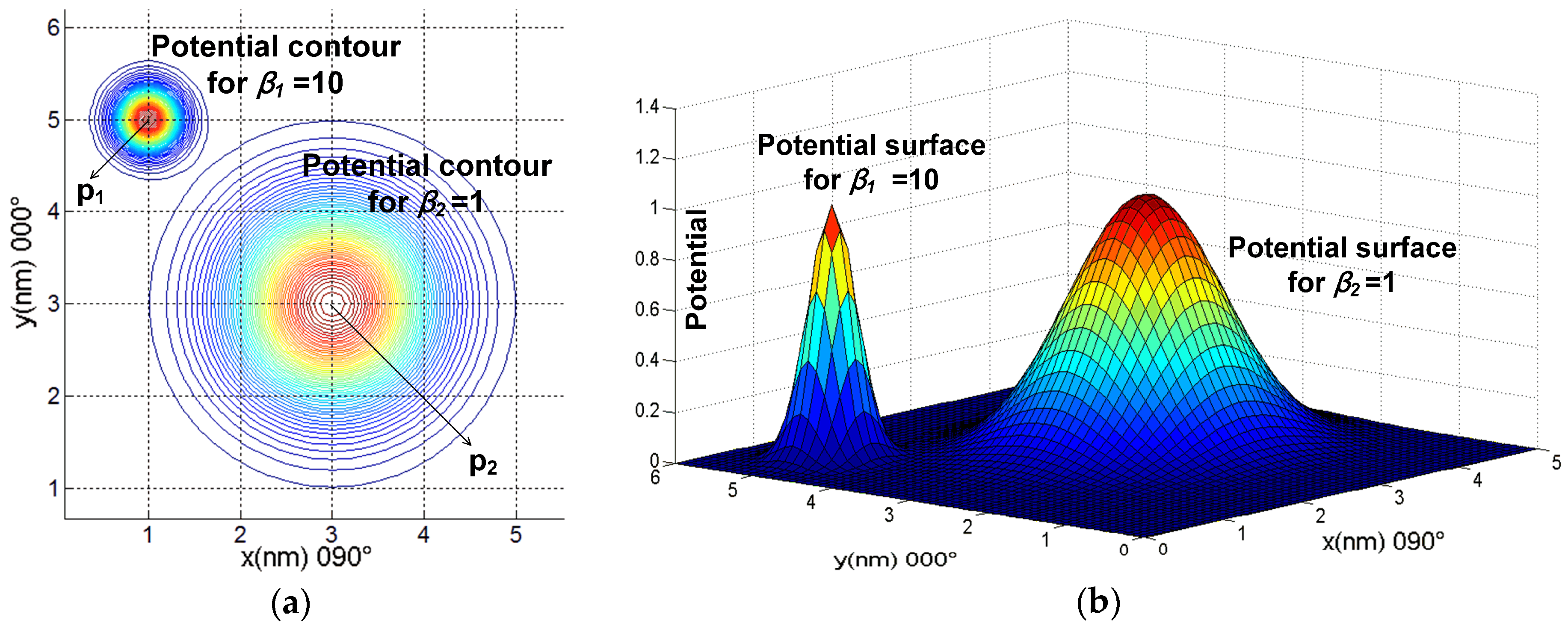
where fpoint(pi) is the potential field function of the i-th point object in position pi(xi, yi), βi is a positive scalar, and fpoint(pi) is a decreasing function of βi. The larger the value of βi is, the faster vanishing and tighter fpoint(pi). When p = pi, the potential will reach the maximum value 1. The larger the distance between the own ship and the point obstacle is, the smaller the effect of the obstacle. This effect approaches 0 at places far away from the obstacle. If there are M (M ∈ N+) point obstacles, the total potential field fpoint(p) can be found by:
Figure 1 shows the total potential field for the two point obstacles p1(1, 5) and p2(3, 3) with different values of parameter β (β1 = 10 and β2 = 1).
For an obstacle in the form of a curve or line c = ϕ(p), the potential field is expressed by the generalized Sigmoid function of c [18]:
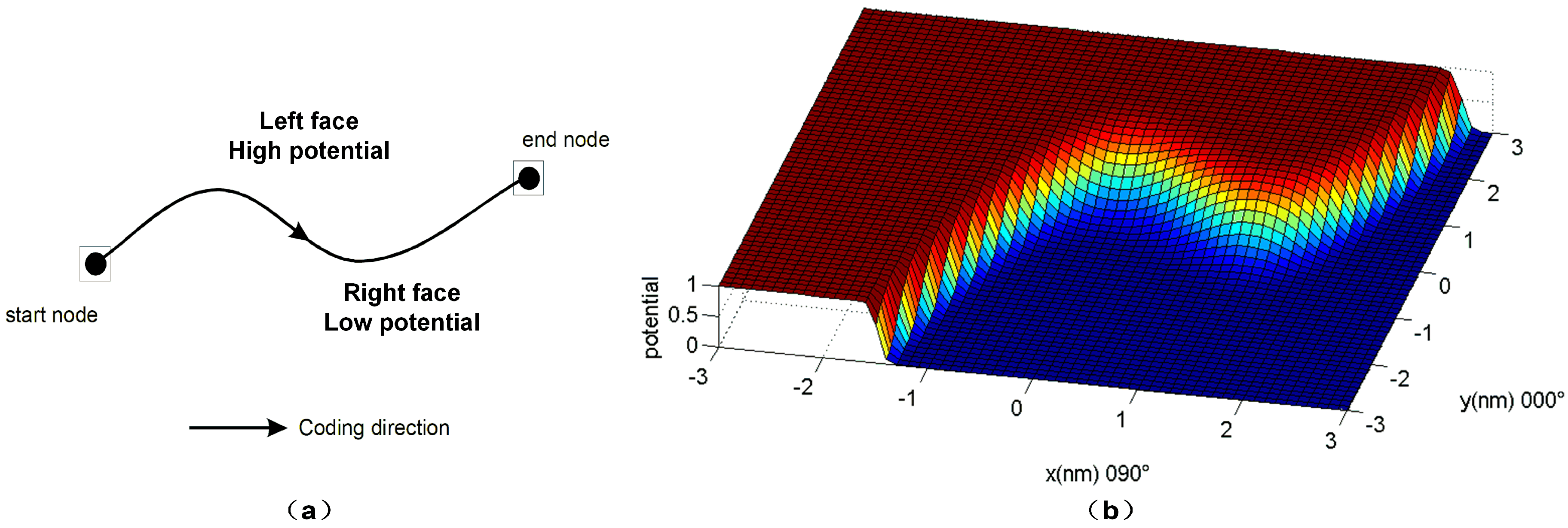
where γ is a positive parameter that is used to adjust the range of influence for the curve obstacle. A small γ leads to a large influence range of an obstacle, but a larger γ makes the influence range of an obstacle smaller. The potential value is 0.5 when the point p(x, y) is exactly on the curve, i.e., c = 0. When c > 0, the potential value is larger, and the maximum is 1. If c < 0, the potential value is smaller, and the minimum value is 0 (far enough from the curve that c = 0). As shown in Figure 2a, based on the coding direction of the curve, the left face of the curve has high potential due to condition c > 0, and the right face is a low potential area due to condition c < 0. The potential field surface for a curve c of −5x3 + 10x2 + x + 10y − 7 = 0 when γ = 0.5 is presented in Figure 2b.
The potential is larger when p(x,y) is on the left face of the curve (c > 0), and it is smaller when p(x,y) is on the right face of the curve (c < 0) based on the coding direction of the curve. The area with a very low potential value is navigable for ships.
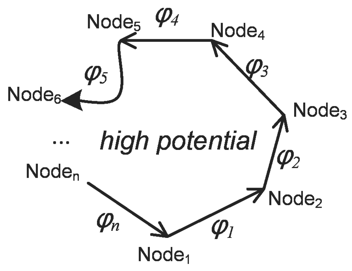
A face (or surface) obstacle consists of n (n ∈ N+) curves that are connected at adjacent nodes and expressed by some implicit functions. The j-th curve is represented by c = ϕj (p). The potential field of the face obstacle fface(p) can be expressed as the product of the Sigmoid function of these curves.
Because any shape can be associated with an implicit function, the selected potential model can make a general representation of obstacles with arbitrary shapes. As shown in Figure 3, according to the counterclockwise coding direction of adjacent nodes, the left faces of the n lines (including curves) have high potential, which constructs a face-shaped obstacle.
It should be noted that formula (4) cannot deal with concave polygons that are totally composed of straight lines. However, we can construct concave polygons in the following ways:
First, the two straight lines forming a concave shape, are replaced by a curve (see Figure 3). Generally, the approximate curve substitute, such as the conic curve and the cubic curve in this paper, can be found and used in the environmental modeling for marine practice.
Second, a concave polygon can also be divided into some convex polygons. Therefore, we can construct the potential field for polygons with concave polygon shapes by adding together the potential fields generated from each of the convex components [18].
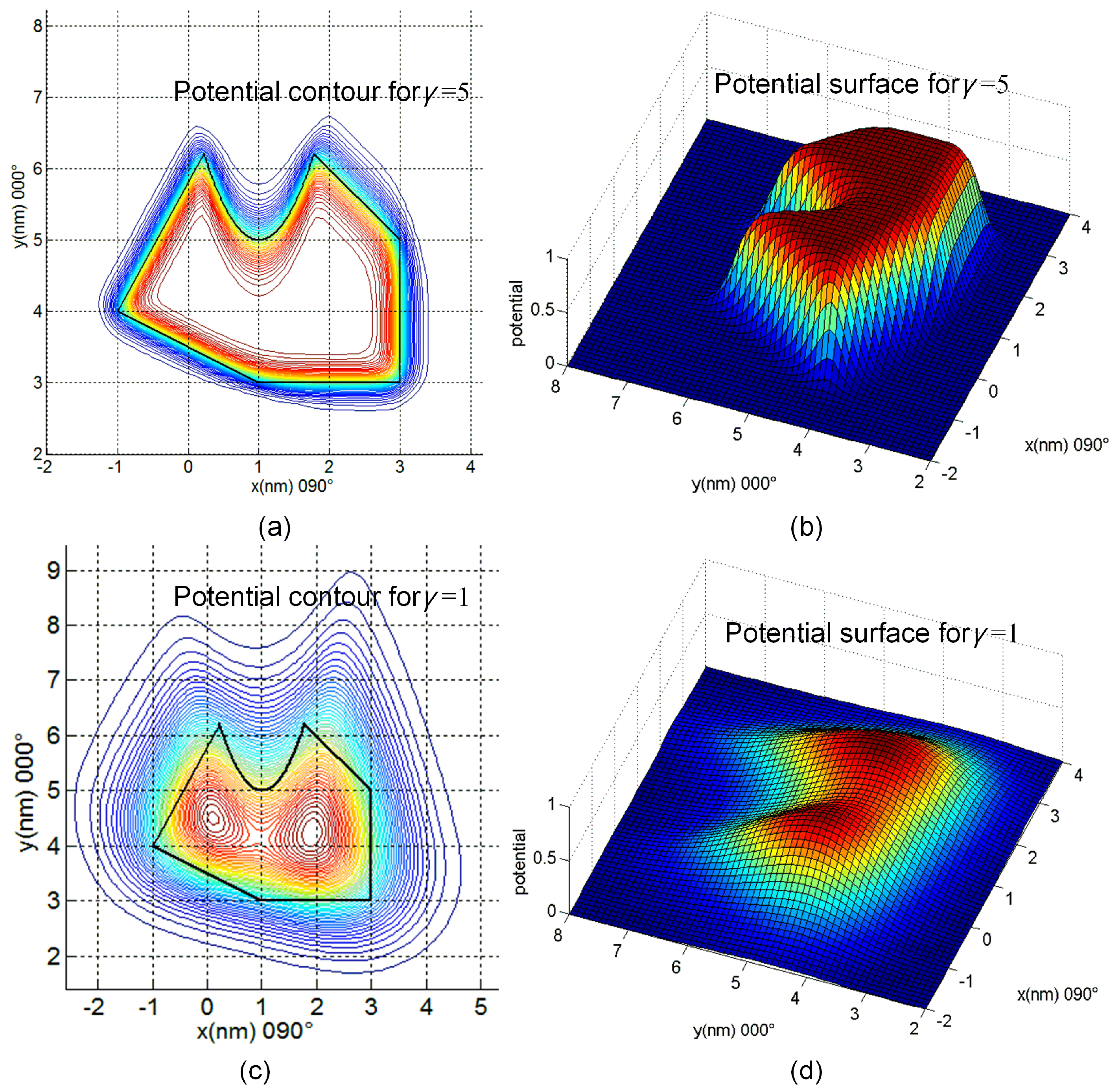
For each face-shaped obstacle, the parameter γ can also be used to adjust the affected area and steepness of the potential field near the edge of the obstacle. A large γ can highly localize the effects of obstacles with low risks and increase the possibility to pass through a narrow passage. A small γ causes large clearance with dangerous obstacles and a large detour or even no passage between two closely located obstacles. Figure 4 shows a face obstacle’s potential field with different values of parameter γ.
The total potential field of the whole static environment can be obtained by adding the potential fields of all the point obstacles, curve obstacles, and face obstacles.
Each type of spatial object may have special features for navigation. It is implied that these objects have a different range of effects to influence path planning for autonomous ships. If the critical value of the obstacle potential range is set to 0.01, the recommended parameters are set in Table 3 based on the safe distance to be maintained with the obstacle. Each side of a surface obstacle can also be set with a different γ based on the feature of the obstacle. For simplicity, this effect is handled with the same parameter γ for a surface obstacle in this table.
2.1.2. Ship Dynamic Properties Modeling
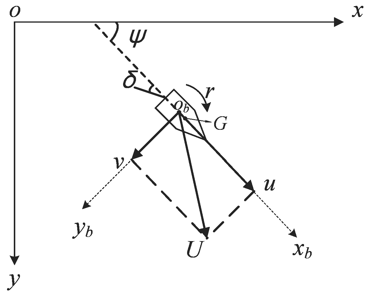
Practical path planning and CA algorithms require precise knowledge about the dynamic properties of a ship. Because the steering of a ship can be regarded as a rigid-body motion on the horizontal plane, a three-degree-of-freedom dynamic model regarding surge, sway and yaw is selected in this paper [12]. The ship maneuvering motion in the earth-fixed and body-fixed coordinate systems is shown in Figure 5, and the relevant equations are as follows:
where m is the mass of the ship, u and v are the surge speed and the sway speed, respectively,
and are the corresponding accelerations, U is the resultant velocity of u and v, ψ, r and represent the yaw angle, yaw rate and yaw acceleration, respectively, and ψ is measured in the inertial frame (). It is assumed that the vessel is symmetric with respect to the centerline, so the center of gravity of the vessel is in the position (xG,0). Iz is the yaw moment of inertia of the vessel, X and Y denote the hydrodynamic forces acting along the axes x and y, respectively, N is the yaw hydrodynamic moment, and δ is the rudder angle.
It can be assumed that X, Y, and N are functions of various state variables and control variable δ. Therefore, X, Y and N can be written as follows:
The use of a third-order truncated Taylor series of the X, Y and N functions will lead to a set of non-linear maneuvering equations for ship motion in the horizontal plane. This is sufficient to show the maneuvering behavior of the vessel. The non-linear model of Mariner class vessels has been discussed by Fossen [19]. In this paper, we choose this model and consider the saturations in the rudder mechanics. The main characteristics of this vessel are described in Table 4. The time required for the ship to turn 90° with maximum rudder angle is 150 s [20].
TSs are assumed to keep their motion parameters or change their course at any point configured by operators. A low-level PD (proportional derivative) controller is incorporated with the governing equations of ship maneuvering:
where δ is the input control variable, Kp is the proportional constant, and Kd is the derivative constant, is the instantaneous yaw angle, i.e., course angle, is the desired course, and r is the yaw rate [21,22].
2.2. Requirements of International Regulations for Preventing Collisions at Sea (COLREGS)
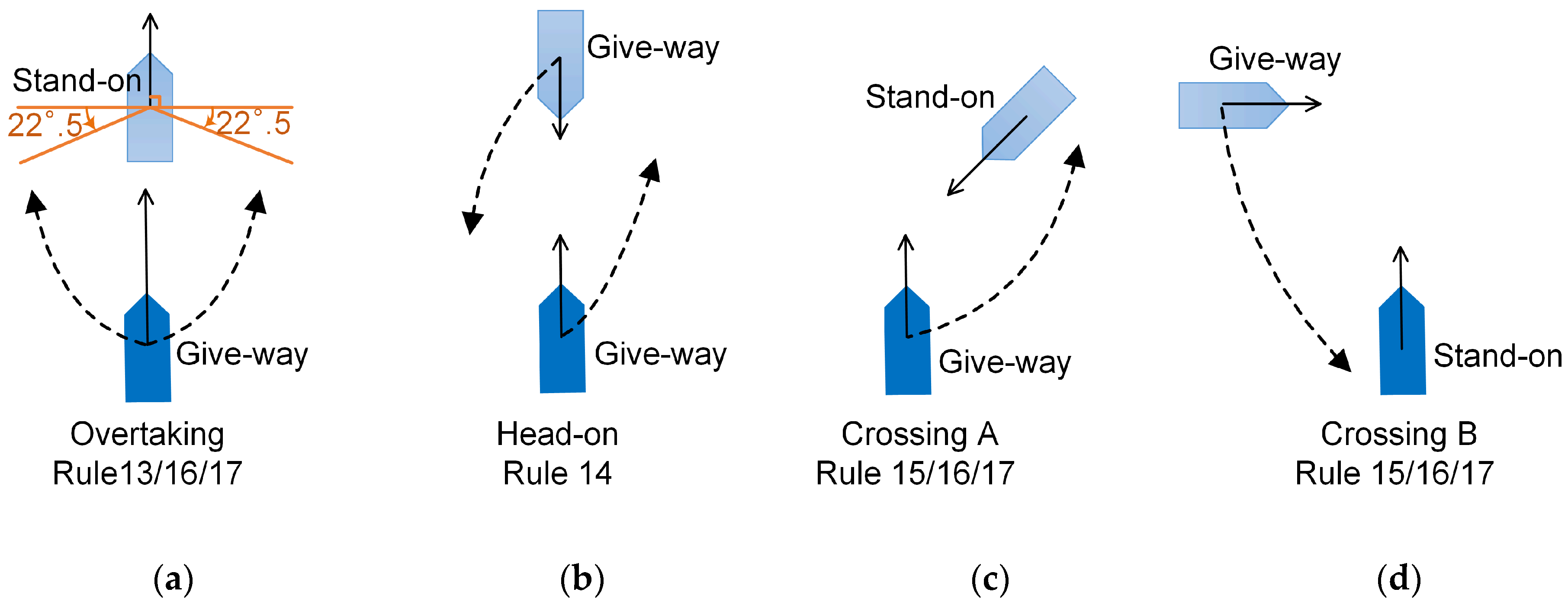
The CA behaviors regulated by COLREGS for two power-driven vessels may be largely characterized as one of three encounters: overtaking (Rule 13), head-on (Rule 14), and crossing (Rule 15) [23], as shown in Figure 6. Rule 13 provides the numerical criteria that “a vessel shall be deemed to be overtaking when coming up with another vessel from a direction of more than 22.5 degrees abaft her beam”. The other two rules have no clear quantification for the arising condition of the corresponding encounters. The overtaking and crossing encounters each identify one vessel as being required to “give-way” (Rule 16) and the other to “stand-on” (Rule 17). The head-on situation requires both vessels to alter course to starboard so that each shall pass on the port side of the other (Rule 14). Rule 16 also requires each give-way vessel to take early and substantial action (course and/or speed change) to keep well clear. A solid arrow indicates the present heading and speed of each vessel, and a dashed arrow indicates the possible direction in which the vessel may take CA action. Speed change is unusual in the practice of navigation except in some emergency situations; therefore, in this paper, course change is assumed as the only strategy adopted for avoiding a collision, which is suitable for the maneuvers of the own ship and all TSs.
2.3. Path Planning Methods
The PGHAPF method, which considers both dynamic and static obstacles, separates the planning into an offline phase and an online phase. By the two steps, this method eliminates the local minima created by static obstacles and acquires a safe path at a high success rate in restricted waters with some moving TSs.
2.3.1. Offline Path Planning for Static Obstacles
In the offline phase, any artificial intelligence (AI) and soft computation method can be utilized to generate a safe and optimal path to the goal in the presence of only static obstacles. Dijkstra’s algorithm [10], the fast marching method (FMM) [14], and the line-of-sight (LOS) method have been used to produce a collision-free and optimal path in a complex environment. However, how to get the path is beyond the content of this paper. It is supposed that the optimal path in the static environment has been obtained. As a prior path, it generally includes a sequence of subgoals or waypoints (WPTs), which is the same as the passage planning on charts undertaken by the bridge team of a vessel. Then, the offline prior path is applied during the online decision-making phase by computing the attractive forces with successive subgoals (WPTs) to guide the USV to the destination unless there is a dynamic obstacle.
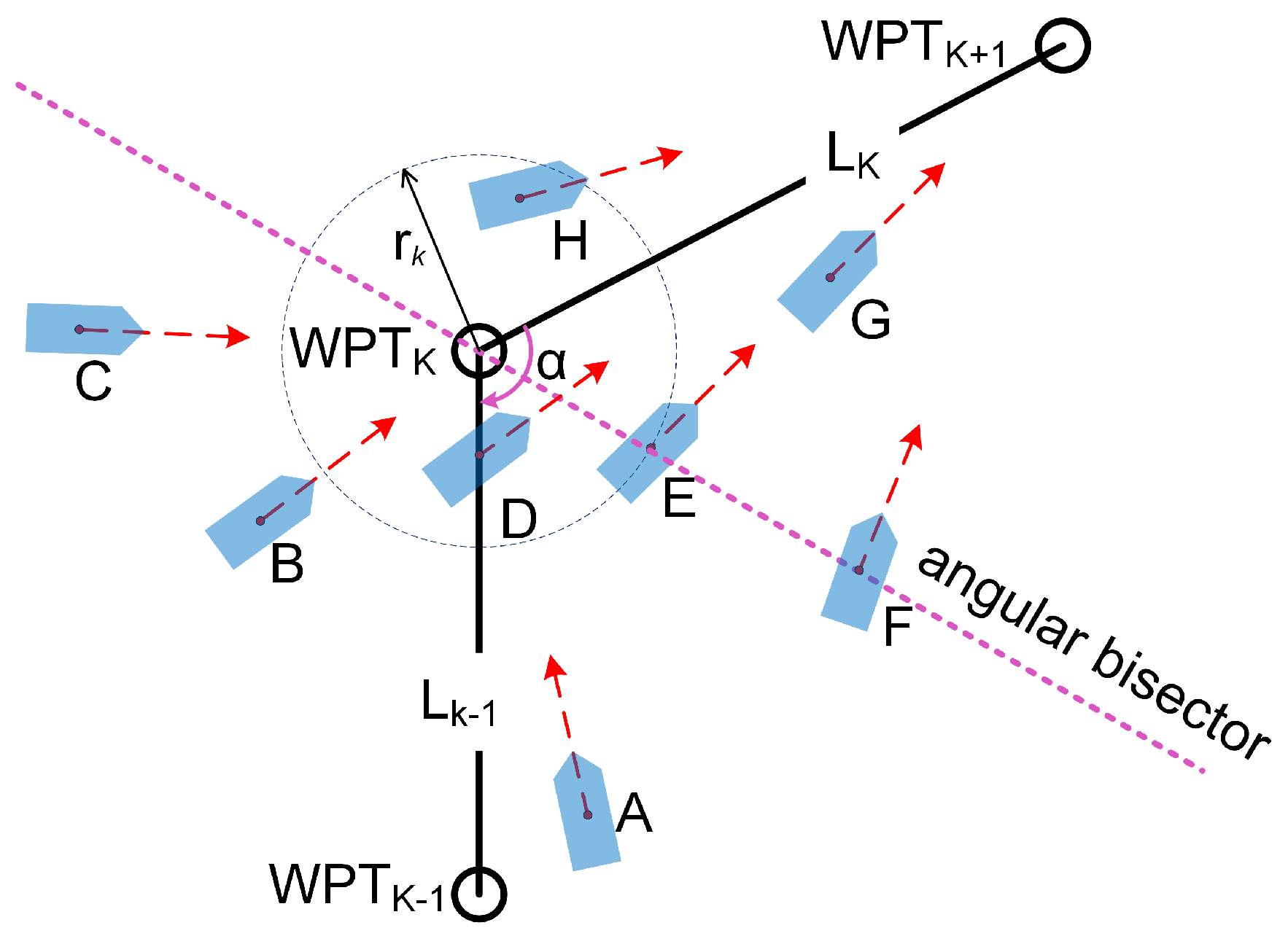
Due to the dynamic environment, it is difficult and impractical for a vessel to sail exactly along the prior path and reach every waypoint. At present, one of the most commonly used methods is to set a circle-of-acceptance (COA) around each waypoint that flags the arrival of the ship at each one [10,24], except the start and end points. As shown in Figure 7, for example, the prior path is composed of 3 WPTs (WPTk−1~k+1) and two legs (Lk−1 and Lk), and the radius of the COA for WPTk is rk. When the distance between the own ship and WPTk (dk) is less than or equal to rk, i.e., the own ship enters the COA of this waypoint (see positions D, E and H), the mission planner selects the next waypoint WPTk+1, and the own ship is guided toward it. However, if the own ship (e.g., at position F) deviates largely near the WPT due to CA actions with other vessels, the dk is always larger than rk, which leads to the failure to complete the leg switch automatically.
In this paper, as a supplementary term to the COA method, a criterion regarding the angular bisector of the angle (α) between the consecutive legs (abbreviated to angular bisector method) is introduced to complete the path leg switch automatically. Before the own ship crosses the angular bisector or the COA (see Figure 7 at positions A, B, and C), the path planning calculations are carried out with reference to leg Lk−1 and subgoal (WPTk), i.e., the end point of Lk−1. When the own ship is passing or has passed the angular bisector (at positions F and G), or enters the COA of the WPTk (at positions D, E and H), the current path leg becomes Lk, and the path planning calculations should be based on WPTk+1 instead of WPTk.
It should be noted that judging whether the own ship has reached the goal or not is still based on the range between the goal and the own ship position; if dg ≤ rg is true, the own ship is considered to have reached the goal.
The prior path-guided process and the automatic selection of waypoints can reduce the risk of trapping the potential function in local minima, optimize the path globally, and extend the application of the APF method to long-distance navigation with many waypoints.
2.3.2. Online Path Planning in Dynamic Environment
The CA decision making for autonomous ships is a complex system that is constrained by COLREGS and should cope with the dynamic environment in real time. The authors have done some work in this field [13]. By considering Rules 13~17 of COLREGS, the CA action scope is divided into four regions, safe zone, negotiation CA zone, emergency CA zone and prohibited zone, according to the checking criterion of collision risk and the checking range (CR) of collision risk. Based on the calculation of repulsive forces under different conditions, a real-time path planning method for static obstacles, dynamic obstacles and an emergency CA module is proposed. The detailed formulas of this algorithm can be referred to in that paper.
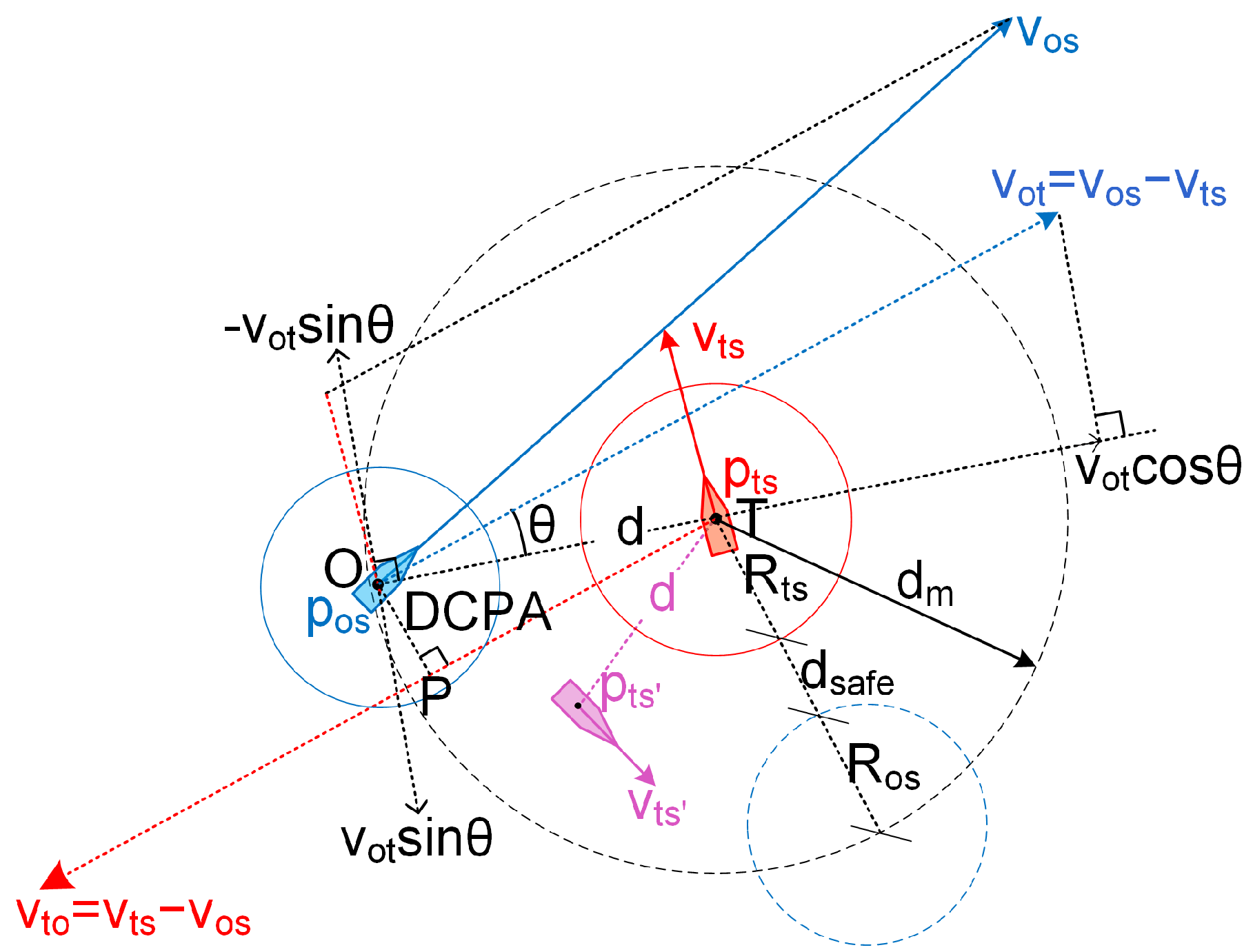
In this paper, we first find that an emergency CA module can be improved by adding a key prerequisite. The checking criterion of collision risk (θ < θm) is no longer applicable once the condition d ≤ dm is true. As shown in Figure 8, d is the distance between the own ship and any TS, dm = Ros + dsafe + Rts, Ros and Rts represent the domain radius of the own ship and TS, respectively, and dsafe is determined by the sea room, position sensor errors, and relative speed of the own ship and TS in one time step. The angle θm does not exist when the own ship position O is in the circle with center T (the position of the TS) and radius dm. In the original algorithm, the condition of emergency CA action for close-range obstacles only has the distance limit d ≤ dm. This condition makes the algorithm calculate the repulsive force for the TSs which have no collision risk with the own ship in this range and, therefore, take unnecessary CA actions. Taking the purple TS′ in Figure 8 as an example, it has a smaller distance (less than dm) from the own ship and is moving away from the own ship. It is obvious that there is no collision risk in this situation, and no necessary CA actions should be taken by the own ship.
Therefore, the algorithm of emergency CA is further improved by adding the judgment about collision risk in this paper. The traditional method for judging collision risk, i.e., the combination of DCPA (distance to the closest point of approach) and TCPA (time to the closest point of approach), is applied in this paper. As shown in Figure 8, DCPA = OP, TCPA = PT/|vto|, and then the prerequisites are written as DCPA ≤ DA and 0 ≤ TCPA ≤ TA, where DA and TA are the limit values determined for the particular sea area [25], which is dependent on the ship’s maneuverability, scale, and visibility, and can be configured by an operator.
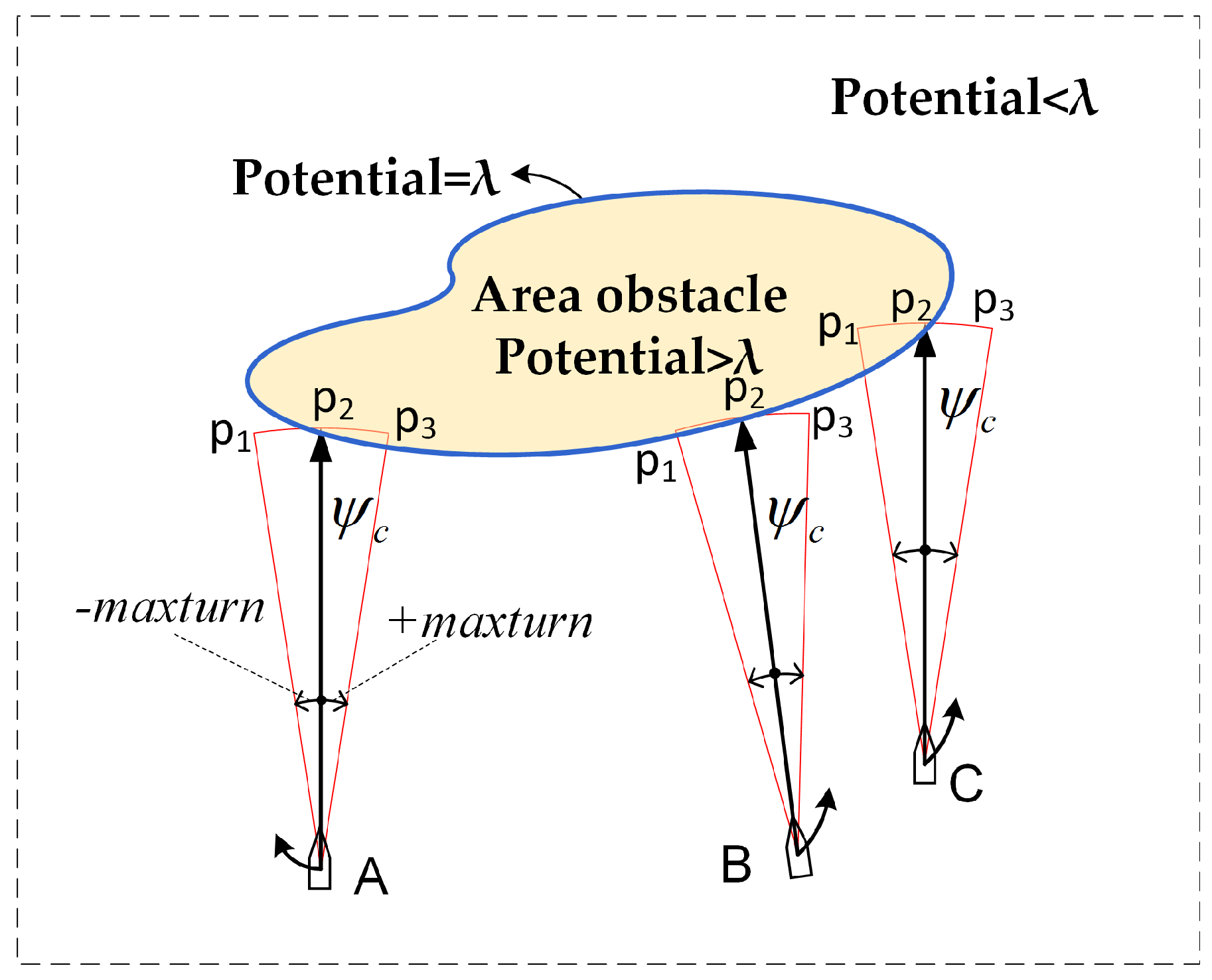
Second, the proposed method in the authors’ previous work [13] can only handle circle-shaped static obstacles. In fact, there may be many static obstacles of various shapes and characteristics surrounding the operational waters of autonomous ships. By using the static environment modeling method described in Section 2.1.1, the potential fields of restricted areas where many static obstacles coexist can be calculated. The higher the potential value (maximum 1) is, the more dangerous it is; the lower the potential value is (minimum 0), the safer it is. Autonomous ships are not allowed to cross or be too close to any static obstacle. Therefore, a minimal potential value λ (e.g., λ = 0.001) may be selected according to the safety requirement, draft, maneuverability and cargo loading condition of the autonomous ship.
As shown in Figure 9, the potential value at the blue boundary of a face obstacle is λ. The potential value is more than λ within this boundary and less than λ outside this boundary. If the potential at the position of the own ship is less than λ, it can be ensured that the own ship does not cross the static obstacle area or keeps a safe distance from it. The current position of the own ship may be A, B or C, and the subsequent position after time tc (e.g., 4 min) is p2 when keeping the current heading ψc. The algorithm continuously calculates the potential value of position p2, i.e., f(p2). If f(p2) ≥ λ, there is a collision risk for the own ship taking the current course, so the necessary course alteration should be taken. The course alteration amplitude at one time step is designed as ± maxturn (“−“ means left turn and “+” means right turn) according to the own ship’s maneuverability. It is supposed that the own ship’s positions after time tc in the two directions ‘ψc + maxturn’ and ‘ψc − maxturn’ are p1 and p3, respectively, and their potential values are written as f(p1) and f(p3). As far as the solution of (9) is obtained, the optimal direction to avoid static obstacles can be determined by the direction of w∗ corresponding to positions p1 and p3. For example, in Figure 9, at the next time step, the own ship should take a left turn at position A and a right turn at positions B and C. Then, the same method is used to acquire the optimal direction to avoid static obstacles at subsequent time steps until all static obstacles are avoided.
2.3.3. Path-Guided Hybrid Artificial Potential Field (PGHAPF) Method
Based on the above, the PGHAPF method proposed in this paper can take into account the global prior path optimization and the influence of the local minimum. In the process of path execution, this method can deal with dynamic TSs and possible irregular static obstacles in advance to take appropriate CA actions in time.
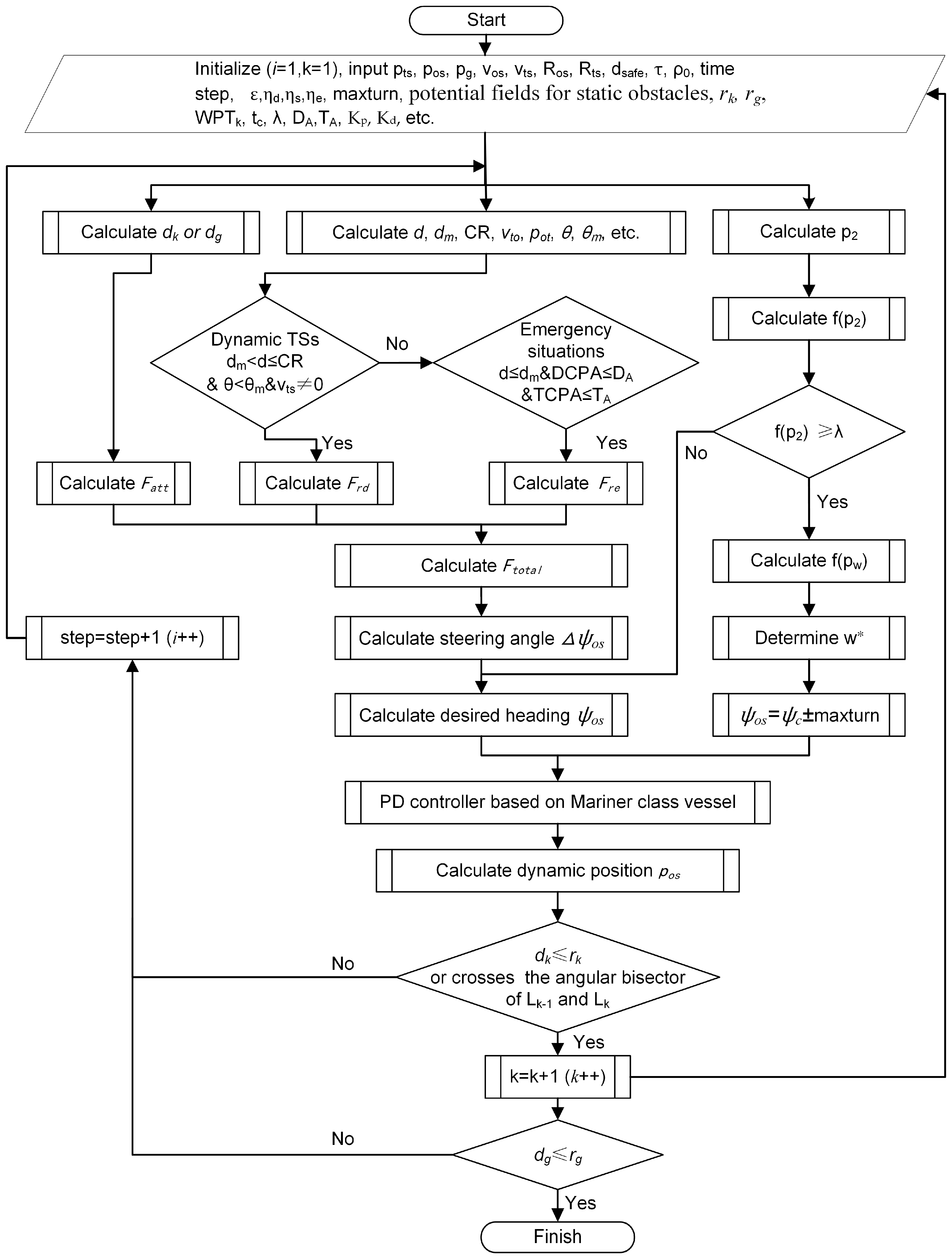
If the prior path is reliable, in the case of no TSs or with TSs but no collision risk, the own ship will be guided only by gravitational force (Fatt) and navigate along the prior path. As shown in Figure 10, when there is any TS that has collision risk with the own ship, the negative gradient of the potential field is calculated. Then, the resultant force (Ftotal), i.e., the sum of repulsive force (Frd) about the relevant TSs and the gravitational force (Fatt) about the goal, is calculated to determine the steering direction of the own ship (ψos) and the dynamic position (pos) in the PD controller. The Frd drives the own ship to avoid all TSs under the COLREGS, and the Fatt makes the own ship move toward the goal or current waypoint WPTk. Once the TS enters the emergency CA zone and meets the emergency CA condition described in Section 2.3.2, the repulsive force for emergency CA (Fre) other than Frd should be calculated to accomplish the successive procedures.
When static obstacles appear suddenly near the prior path or the own ship deviates from the prior path due to the action of avoiding TSs, these nearby static obstacles may lead to a new danger for the own ship, especially in restricted waters. Because of the non-cooperative feature of static obstacles, this algorithm gives higher priority of CA to static obstacles. No matter what the precondition is, when a static obstacle is encountered in front of the own ship (i.e., f(p2) ≥ λ), the minimum potential following method shown in Figure 9 is used to calculate the steering direction (ψos) of the own ship. Once the danger originated by a static obstacle is eliminated, that is, f(p2) < λ, the algorithm next determines ψos by calculating the negative gradient and resultant force (Ftotal) of the potential field that is formed by dynamic TSs and the goal or current waypoint.
When the distance between the own ship and WPTk dk ≤ rk, or when the own ship has crossed or is crossing the angular bisection of the angle composed of path legs Lk−1 and Lk, it is deemed that the current waypoint WPTk has been reached, and then the next waypoint WPTk+1 is the new goal point. When the distance to the final goal dg ≤ rg, the algorithm loop will terminate. Figure 10 shows a flowchart of the PGHAPF method, where some variables refer to the authors’ previous work [13] except those stated in this paper.
3. Results
To show the merits of this approach, some well-designed simulations were conducted using a PC with an Intel Core i5 3230m 2.6 GHz processor, 12 GB RAM, and a 64-bit Windows 7 Professional operating system. The following global parameters were used in these simulations: ε = 3000, ηd = 2000, ηs = 300,000, ηe = 2000, τ = 0.3 nautical mile (nm), λ = 0.001, Ros = 0.5 nm, dsafe = 1 nm, ρo = 3~5 nm, maxturn = 5°, DA = 0.3 nm, TA = 6 min, rk = rg = 0.25 nm, tc = 4 min, Kp = 1, Kd = 10 and time step = 15 s. It should be noted that these parameters should be adjusted according to specific ship dynamics in real operations.
The results are illustrated in multiple figures, representing snapshots of situations. A two-dimensional Cartesian coordinate system presents the distance in nautical miles (nm); the vertical axis in the positive direction shows North 000°, and the horizontal axis in the positive direction is 090°. The following symbols and color codes are applied:
- The black dotted line with the red box as the starting point and the blue triangle as the endpoint is the resulting trajectory of the own ship, and the green line is the prior path of the own ship, which may be short but not necessarily safe.
- To illustrate the CA actions with dynamic TSs, the own ship heading at every time step is plotted with a blue dot, which makes it easy to find the course alteration points.
- The paths of multiple TSs are identified by corresponding TS numbers and different colors.
- The range (scope 0~6 nm) between the own ship and any TS at each time step is chosen to display in various colors.
- The paths of the own ship and all TSs are labeled at regular intervals of 50 time steps.
- The boundary contours of static obstacles are black solid lines, whose potential field is colored from red (high potential) to blue (low potential) and is drawn at an interval of 0.01.
3.1. Simulations for Static Obstacles
First, we simulate the automatic path planning for the own ship in the presence of irregular static obstacles without designating a prior collision-free path to verify the effectiveness of the proposed algorithm in solving the problems in traditional APF methods.
3.1.1. Trap Situations in U-shaped Obstacles and the Goals Non-Reachable with Obstacles Nearby (GNRON) Problem
This simulation is designed to verify the feasibility of the proposed algorithm for the local minima problem and the GNRON problem of the traditional APF method [10,26]. The initial state of the own ship and the results are shown in Table 5 and Figure 11.
These two simulations have a very short total running time of 0.4–0.5 s in 10 repeated trials.
3.1.2. No Passage through Closely Spaced Obstacles and Oscillations in Narrow Passages
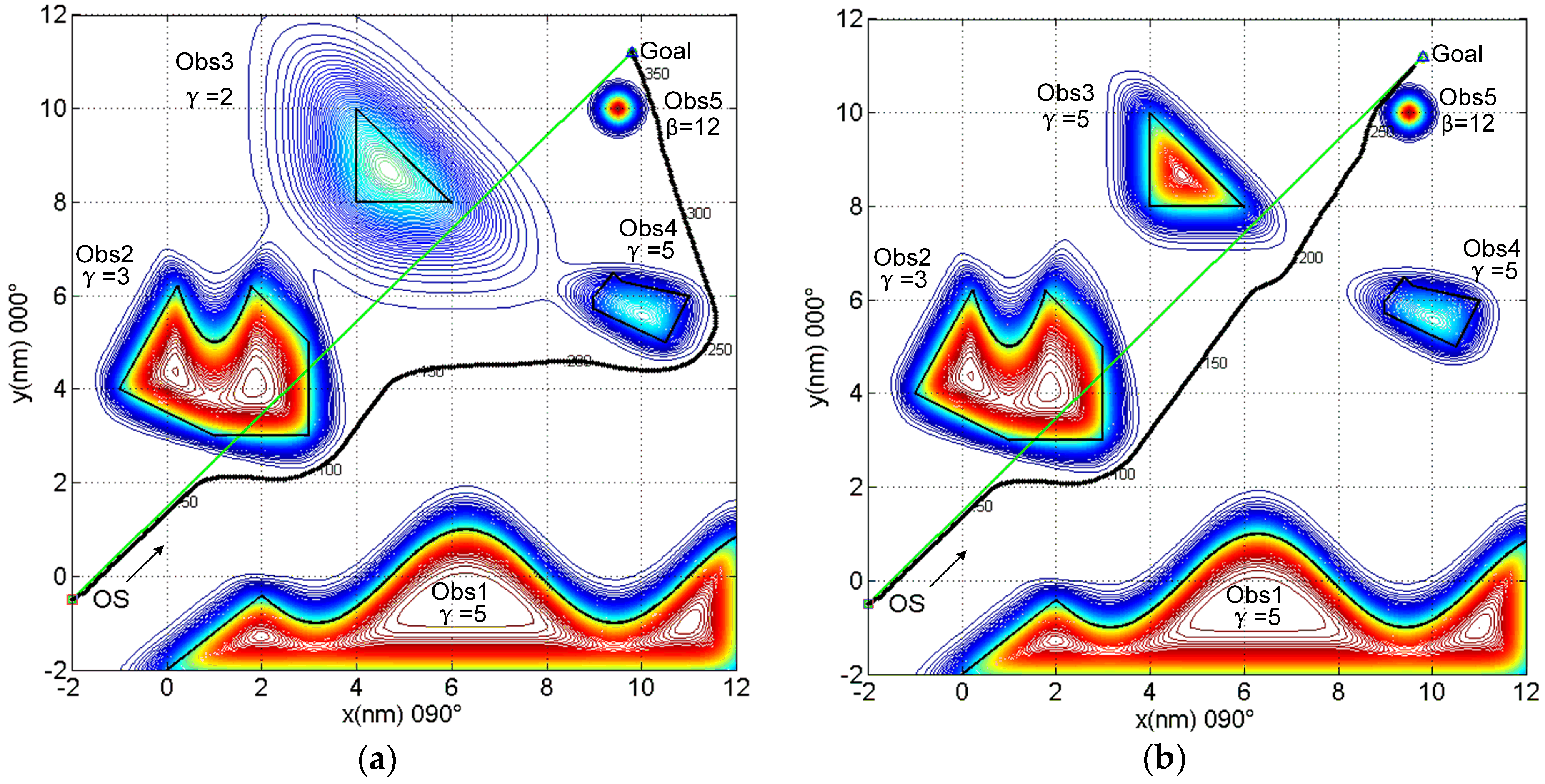
This simulation is designed for the algorithm to handle more obstacles with narrow channels, especially for the conditions of no passage through closely spaced obstacles and oscillations in narrow passages. The static environment consists of five kinds of static obstacles with different shapes (combined curve, combined polygon, concave polygon, triangle and point). Their actual boundaries are marked by black solid lines, and their characteristics and potential parameters are shown in Figure 12. The initial states and results of the simulations are shown in Table 6.
These two experiments keep safe distances from static obstacles, and there are no oscillations in passages. The total simulation time is very short, approximately 0.6 s in 10 repeated trials.
3.2. Simulations for Emergency Scenarios with a Dynamic Target Ship (TS)
CA simulation results for three typical encounters between two ships were described in [13]. This simulation is only used to verify the improvement in the emergency CA module. Taking the head-on situation as an example, the initial conditions for the two ships are shown in Table 7. The simulation results before and after the improvement are compared in Figure 13.
Finally, the results of the two methods are compared in Table 8.
3.3. Simulations in Complex Environment
On the basis of five kinds of static obstacles in Figure 12b, four dynamic TSs are added to the restricted waters. Additionally, four typical encounter situations are designed in this simulation. The start point of the own ship, waypoints of the prior path, and the final goal are (−2, −0.5), (4.5, 2.5), (10.4, 9.7) and (9.8, 11.2), respectively, and the speed of the own ship is 15 kn. The initial input of test data for each TS, such as pts (start point), vts (speed), and Rts (domain radius), as well as the encounter situation with the own ship, the CA actions taken by the own ship, and the final DCPA, are represented in Table 9. Screenshots of important situations in the simulation are shown in Figure 14, Figure 15, Figure 16 and Figure 17a,b and Video S1 (see Supplementary Materials).
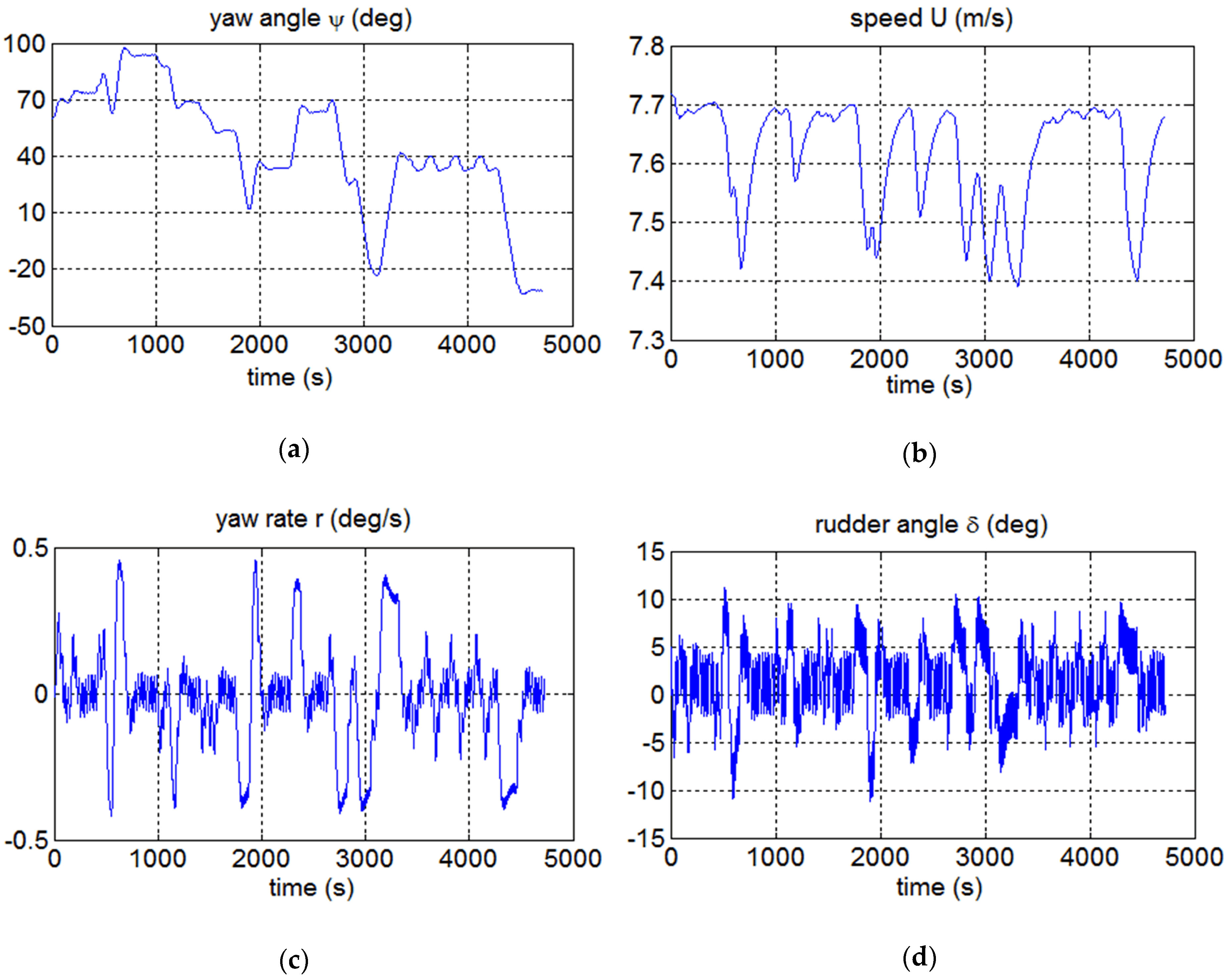
In addition to the above snapshots, this simulation shows that the total trajectory length is 19.38 nm, and the total time steps are 315, which corresponds to 4725 s in reality. This simulation result is unique in 10 more repeats due to this deterministic algorithm. Only the total running time of the simulation that is in the interval of 0.804–0.833 s has a small difference. Furthermore, the real-time manipulation data obtained by a PD controller are shown in Figure 18a–d.
4. Discussion
When an autonomous ship is navigating according to the planned path, she will inevitably encounter dynamic TSs. Once the collision risk is detected, she should take actions under applicable regulations such as COLREGS, and she may deviate from the planned path temporarily due to her give-way obligations in some encounter situations. This may lead to collision risk with surrounding static obstacles, especially in restricted waters. Therefore, she needs to consider all static and dynamic obstacles at the same time and then make a fast, feasible and comprehensive decision. However, many studies are based on the following test environments or assumptions:
Therefore, a fast path planning algorithm is designed and tested as above that is constrained by a ship’s dynamic properties, COLREGS and planned route and can consider many irregular static obstacles, multiple dynamic TSs and their uncoordinated CA operations at the same time.
First, the PGHAPF method can avoid static obstacles with arbitrary shapes (including points, lines, and planes) in addition to the ability to avoid dynamic TSs under COLREGS. There are three key steps for this method:
- the potential-based method to model the environment for any irregular static obstacles. Very simple parameters such as β or γ can be adjusted to change the range of the potential field of obstacles with different attributes, which is convenient for environmental modeling with ENC data in the future.
- the gradient-based method to produce the COLREGS-constrained repulsive forces for dynamic TSs and the attractive force for the goal, which is achieved in [13] and improved in this paper for the emergency CA module.
- the PGHAPF method, which is a fusion of the potential field and gradient methods (the above two) based on a prior path, is proposed first in this paper. Under the static potential field, a decision-making time in advance is selected according to the surroundings and speed of the own ship to determine whether there is danger at the predetermined position. If there is, the own ship turns right or left with maxturn angle at the current time step, which is dependent on the direction of the minimum potential location referring to the predetermined position. Otherwise, the own ship takes the actions based on the second step. This method can effectively reduce the local minima problem of the traditional APF method caused by the vector sum of attractive and repulsive forces. It can avoid concave static obstacles in advance and reach the goal with obstacles nearby, other than being trapped in U-shaped obstacles (see Figure 11 and Figure 12). It should be noted that the decision-making time should be adjusted suitably; although a larger value can make early CA actions possible, it may skip some small obstacles.
Second, a three-degree-of-freedom Mariner class vessel is incorporated in this method, providing more realistic trajectories that are closely followed by the autopilot. The desired heading of each time step, which is calculated by the main part of the algorithm, is taken as the input of the PD controller. The output of the PD controller, including the ship’s real-time position, speed, yaw rate and rudder angle, is treated as the input of the path planning for the next time step. After many iteration cycles, a practical and smooth path is produced.
Third, the marine environment is complex and changeable, including the influence of winds and current and the steering instability of a ship. It is difficult to strictly maintain course and speed for any TS. Additionally, the TS may be approaching the next waypoint, avoiding static obstacles or making way for other TSs. Of course, most ships take CA actions in accordance with COLREGS, but COLREGS do not quantify the timing and magnitude of the CA actions regarding course and/or speed change, etc. Different operators have different understandings of COLREGS because of different navigation experiences. Therefore, it is not easy to accurately predict the possible COLREGS-compliant actions (including their magnitude), especially in multiship encounters. There is even a risk that some TSs will not obey COLREGS and seafarers’ usual practice. Therefore, our method has as its priority compliance with rules 13–17 of COLREGS for power-driven vessels (see Table 9 and Figure 17). In addition, the proposed method reacts immediately to sudden changes such as the uncoordinated CA behaviors of TSs and is capable of improving the quality of output plans by automatically judging and handling the surrounding obstacles (see Figure 13 and Figure 16).
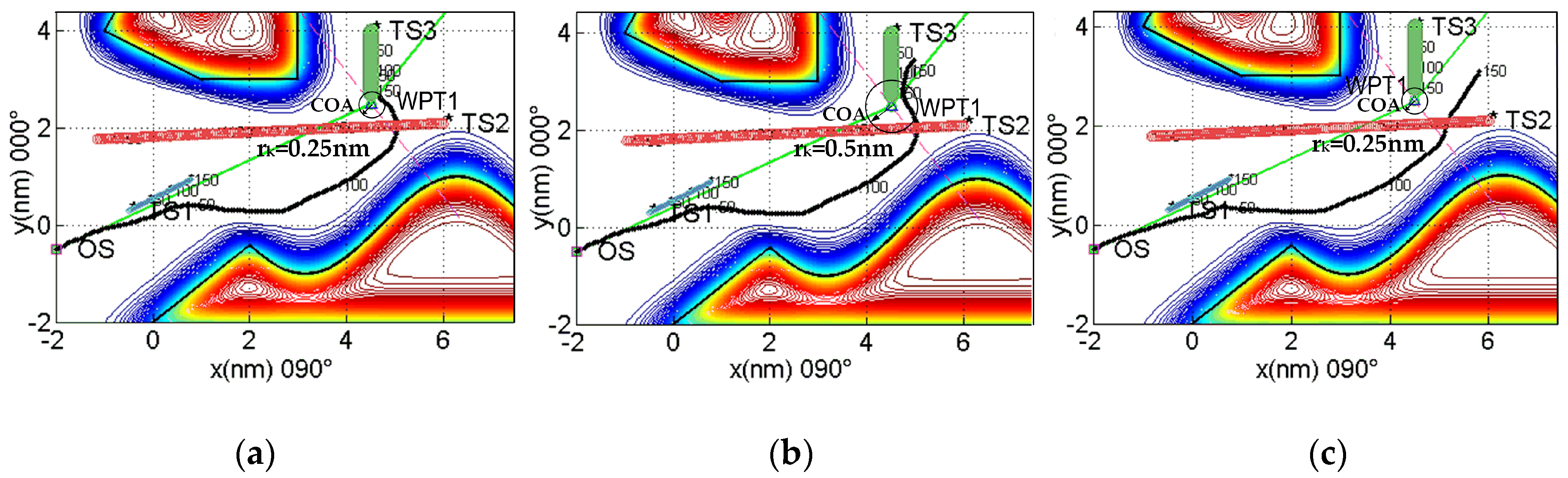
Fourth, we introduce a modified WPT selection method, i.e., the angular bisector method based on the prior path planning algorithm. By doing this, the method of COA is improved to avoid extra detour or collision risk when some obstacles are in the vicinity of the waypoint. Figure 19a shows a collision example with TS3 when rk = 0.25 nm without adopting the angular bisector method. A larger rk may solve the collision problem, but it will lead to a larger detour from the prior path (see Figure 19b), where rk = 0.5 nm without using the angular bisector method. Our method can make the own ship navigate along a long optimal path with multiple waypoints and adjust them automatically by reacting to dynamic environments. As shown in Figure 19c, the own ship would cause danger to dynamic TS3 if she continues approaching WPT1. After crossing the angular bisector of the angle between the adjacent path legs, the next waypoint WPT2 rather than WPT1 is automatically selected as the subgoal, although the own ship position is not in the COA of WPT1. This simulation demonstrates the flexibility and optimization ability of the proposed method in path planning.
Therefore, the test assumptions and environments in this paper can match the real navigation environments of autonomous ships to a certain extent. In addition, the PGHAPF method has the following advantages.
This method requires very low computational time. The total run time can be 0.8 s for a simulation with dynamic and complex environments, whose planning distance is 19.38 nm with a total of 315 time steps. Thus, the decision-making time for one time step is only approximately 2.6 milliseconds (ms). The running times of other experiments are shown in Table 10. The computational time of the PGHAPF method is not obviously affected by the number of obstacles or planning distance, but it may be influenced by the complexity of construction for the obstacle APF. This method can meet the real-time requirements of CA decision-making systems for autonomous ships.
This method is a deterministic path planning algorithm. It computes the collision-free path in a dynamic environment based on the prior path and the complete theory about the potential field and gradient. The calculation is simple, the parameter setting is clear, and the calculation solution is reliable. Each test was repeated many times, and the solution was unique under the same test conditions. This is an important property in CA decision-making systems for autonomous ships. For some stochastic-based algorithms, the convergence of a solution might not be guaranteed due to the presence of random variables.
Lastly, there are still some shortcomings in this method. For instance, the own ship is given a priority to keep out of the way of other ships and fewer obligations to be a stand-on ship. The algorithm does not consider speed changes in CA actions for the own ship as well as some extreme conditions such as stopping or reversing her means of propulsion. Without considering external disturbances of wind, waves, current and other natural conditions, the APF model of static obstacles needs implicit functions that may be acquired by curve fitting based on the data extraction of the ENC.
5. Conclusions
The PGHAPF method proposed in this paper can quickly plan a deterministic collision-free path in the presence of a variety of static obstacles with arbitrary shapes and multiple dynamic ships with variable headings. This method takes into account the constraints of COLREGS, the dynamics of a Mariner class vessel, and the results of offline path planning and can adjust the path immediately according to a change in the dynamic environment, including the uncoordinated CA actions of other ships and the collision risk with nearby static obstacles caused by path adjustment. Additionally, a simple waypoint selection scheme is implemented together with the PGHAPF method to obtain a more optimized path and avoid danger. The results show the potential to perform path planning on ECDIS and to overcome the inherent defects of APF methods, such as the local minima, GNRON and oscillations in narrow passages. Furthermore, the PGHAPF method may be used in the fields of USVs, AUVs (autonomous underwater vehicles) and robots.
There are some directions in which to expand our work. First, the CA actions taken by ships should not be limited to course change only. Multiship encounter situations may be further quantified and judged to acquire COLREGS-compliant behaviors accurately for autonomous ships. Furthermore, the potential field model for static obstacles is planned to be integrated into ECDIS so that the PGHAPF method can be validated in a more real-life experiment.
Supplementary Materials
The following is available online at https://www.mdpi.com/2076-3417/8/12/2592/s1: Video S1: COLREGS-constrained PGHAPF method navigating an autonomous ship in a complex environment with 5 arbitrary static obstacles and 4 other dynamic ships.
Author Contributions
Conceptualization, H.L. and Y.Y.; Methodology, H.L.; Software, H.L.; Validation, H.L. and Y.Y.; Writing-Original Draft Preparation, H.L.; Writing-Review and Editing, H.L. and Y.Y.; Visualization, H.L.; Funding Acquisition, H.L. and Y.Y.
Funding
This research was funded by Traffic Youth Science and Technology Talent Project grant number 36260401, Natural Science Foundation of Liaoning Province of China grant number 201602081 and Fundamental Research Funds for the Central Universities grant number 3132018306.
Conflicts of Interest
The authors declare no conflict of interest.
List of Acronyms
| AI | artificial intelligence |
| APF | artificial potential field |
| APF-SR | artificial potential field - stochastic reachable |
| AUV | autonomous underwater vehicle |
| BEA | bacterial evolutionary algorithm |
| BPF | bacterial potential field |
| CA | collision avoidance |
| COA | circle-of-acceptance |
| COLREGS | International Regulations for Preventing Collisions at Sea |
| CPP | cooperative path planning |
| CR | checking range |
| DCPA | distance to the closest point of approach |
| EA | evolutionary algorithm |
| ECDIS | electronic chart display information systems |
| ENC | electronic navigational chart |
| FL | fuzzy logic |
| FMM | fast marching method |
| GNRON | goals non-reachable with obstacles nearby |
| LOS | line-of-sight |
| MPC | model predictive control |
| PD | proportional derivative |
| PGHAPF | path-guided hybrid artificial potential field |
| RAM | random access memory |
| SOM | self-organizing map |
| SPS | scalar potential surface |
| TBA | trajectory base algorithm |
| TCPA | time to the closest point of approach |
| TS | target ship |
| USV | unmanned surface vehicle |
| WPTs | waypoints or successive subgoals |
References
- Szlapczynski, R. Evolutionary Sets of Safe Ship Trajectories a New Approach to Collision Avoidance. J. Navig. 2011, 64, 169–181. [Google Scholar] [CrossRef]
- Tam, C.; Bucknall, R. Cooperative path planning algorithm for marine surface vessels. Ocean Eng. 2013, 57, 25–33. [Google Scholar] [CrossRef]
- Lazarowska, A. A new deterministic approach in a decision support system for ship’s trajectory planning. Expert Syst. Appl. 2017, 71, 469–478. [Google Scholar] [CrossRef]
- Tam, C.; Bucknall, R. Path-planning algorithm for ships in close-range encounters. J. Mar. Sci. Technol. 2010, 15, 395–407. [Google Scholar] [CrossRef]
- Brcko, T.; Svetak, J. Fuzzy Reasoning as a Base for Collision Avoidance Decision Support System. Promet-Traffic Transp. 2013, 25, 555–564. [Google Scholar] [CrossRef] [Green Version]
- Lee, S.M.; Kwon, K.Y.; Joh, J. A fuzzy logic for autonomous navigation of marine vehicles satisfying COLREG guidelines. Int. J. Control Autom. Syst. 2004, 2, 171–181. [Google Scholar]
- Lazarowska, A. Ship’s Trajectory Planning for Collision Avoidance at Sea Based on Ant Colony Optimisation. J. Navig. 2015, 68, 291–307. [Google Scholar] [CrossRef]
- Szlapczynski, R. Evolutionary Planning of Safe Ship Tracks in Restricted Visibility. J. Navig. 2015, 68, 39–51. [Google Scholar] [CrossRef]
- Johansen, T.A.; Perez, T.; Cristofaro, A. Ship Collision Avoidance and COLREGS Compliance Using Simulation-Based Control Behavior Selection With Predictive Hazard Assessment. IEEE Trans. Intell. Transp. Syst. 2016, 17, 3407–3422. [Google Scholar] [CrossRef] [Green Version]
- Chiang, H.T.; Malone, N.; Lesser, K.; Oishi, M. Path-guided artificial potential fields with stochastic reachable sets for motion planning in highly dynamic environments. In Proceedings of the 2015 IEEE International Conference on Robotics and Automation (ICRA), Seattle, WA, USA, 26–30 May 2015; pp. 2347–2354. [Google Scholar]
- Ge, S.S.; Cui, Y.J. New potential functions for mobile robot path planning. IEEE Trans. Robot. Autom. 2000, 16, 615–620. [Google Scholar] [CrossRef]
- Xue, Y.; Clelland, D.; Lee, B.S.; Han, D. Automatic simulation of ship navigation. Ocean Eng. 2011, 38, 2290–2305. [Google Scholar] [CrossRef]
- Lyu, H.; Yin, Y. COLREGS-Constrained Real-time Path Planning for Autonomous Ships Using Modified Artificial Potential Fields. J. Navig. 2018. [Google Scholar] [CrossRef]
- Liu, Y.; Bucknall, R. Efficient multi-task allocation and path planning for unmanned surface vehicle in support of ocean operations. Neurocomputing 2018, 275, 1550–1566. [Google Scholar] [CrossRef]
- Montiel, O.; Orozco-Rosas, U.; Sepúlveda, R. Path planning for mobile robots using Bacterial Potential Field for avoiding static and dynamic obstacles. Expert Syst. Appl. 2015, 42, 5177–5191. [Google Scholar] [CrossRef]
- Bayat, F.; Najafi-Nia, S.; Aliyari, M. Mobile Robots Path Planning: Electrostatic Potential Field Approach. Expert Syst. Appl. 2018, 100, 68–78. [Google Scholar] [CrossRef]
- Pietrzykowski, Z.; Magaj, J.; Mąka, M. Safe Ship Trajectory Determination in the ENC Environment. In Proceedings of the International Conference on Transport Systems Telematics, Ustron, Poland, 22–25 October 2014; pp. 304–312. [Google Scholar]
- Ren, J.; McIsaac, K.A.; Patel, R.V.; Peters, T.M. A Potential Field Model Using Generalized Sigmoid Functions. IEEE Trans. Syst. Man Cybern. B Cybern. 2007, 37, 477–484. [Google Scholar] [CrossRef] [PubMed]
- Fossen, T.I. Guidance and Control of Ocean Vehicles; Wiley: Chichester, UK, 1994. [Google Scholar]
- Lin, X. Model Research on Automatic Collision Avoidance of Ships in Confined Waterways Based on Improved Improved Potential Field Method; Harbin Engineering University: Harbin, China, 2015. [Google Scholar]
- Chiang, H.T.L.; Tapia, L. COLREG-RRTT: An RRT-Based COLREGS-Compliant Motion Planner for Surface Vehicle Navigation. IEEE Robot. Autom. Lett. 2018, 3, 2024–2031. [Google Scholar] [CrossRef]
- Lee, G.; Surendran, S.; Kim, S.H. Algorithms to control the moving ship during harbour entry. Appl. Math. Model. 2009, 33, 2474–2490. [Google Scholar] [CrossRef]
- Woerner, K.; Novitzky, M. Legibility and Predictability of Protocol-Constrained Motion: Evaluating Human-Robot Ship Interactions Under COLREGS Collision Avoidance Requirements. In Proceedings of the Robotics Science and Systems, Cambridge, MA, USA, 12–16 July 2017. [Google Scholar]
- Naeem, W.; Irwin, G.W.; Yang, A. COLREGs-based collision avoidance strategies for unmanned surface vehicles. Mechatronics 2012, 22, 669–678. [Google Scholar] [CrossRef]
- Hilgert, H.; Baldauf, M. A common risk model for the assessment of encounter situations on board ships. Deutsche Hydrogr. Z. 1997, 49, 531–542. [Google Scholar] [CrossRef]
- Ge, S.S.; Cui, Y.J. Dynamic Motion Planning for Mobile Robots Using Potential Field Method. Auton. Robot. 2002, 13, 207–222. [Google Scholar] [CrossRef]
- Zhao, Y.; Li, W.; Shi, P. A real-time collision avoidance learning system for Unmanned Surface Vessels. Neurocomputing 2016, 182, 255–266. [Google Scholar] [CrossRef]
- Gia Huy Dinh, N.I. A Study on the Construction of Stage Discrimination Model and Consecutive Waypoints Generation Method for Ship’s Automatic Avoiding Action. Int. J. Fuzzy Log. Intell. Syst. 2017, 17, 294–306. [Google Scholar] [CrossRef] [Green Version]
- Tsou, M.C. Multi-target collision avoidance route planning under an ECDIS framework. Ocean Eng. 2016, 121, 268–278. [Google Scholar] [CrossRef]
- Benjamin, M.R.; Curcio, J.A.; Leonard, J.J.; Newman, P.M. Navigation of unmanned marine vehicles in accordance with the rules of the road. In Proceedings of the IEEE International Conference on Robotics and Automation, Orlando, FL, USA, 15–19 May 2006; pp. 3581–3587. [Google Scholar]
Figure 1.
(a) The potential contours of the total potential field for two point obstacles with different values of parameter β. (b) The corresponding potential surface of the total potential field.
Figure 1.
(a) The potential contours of the total potential field for two point obstacles with different values of parameter β. (b) The corresponding potential surface of the total potential field.

Figure 2.
(a) The potential features for a curve with the coding direction. (b) The surface of a potential field for a curve-shaped obstacle.
Figure 2.
(a) The potential features for a curve with the coding direction. (b) The surface of a potential field for a curve-shaped obstacle.

Figure 3.
Construct diagram for a potential field of face or surface elements.

Figure 4.
Potential field for a complex face obstacle with different values of parameter γ. (a) and (b) are potential contours and potential surface for γ = 5 respectively. (c) and (d) are potential contours and potential surface for γ = 1 respectively.
Figure 4.
Potential field for a complex face obstacle with different values of parameter γ. (a) and (b) are potential contours and potential surface for γ = 5 respectively. (c) and (d) are potential contours and potential surface for γ = 1 respectively.

Figure 5.
Coordinate system of ship maneuvering motion.

Figure 6.
Typical encounters illustration: (a) overtaking, (b) Head-on, (c) crossing A and (d) crossing B and the corresponding Rules in COLREGS.
Figure 6.
Typical encounters illustration: (a) overtaking, (b) Head-on, (c) crossing A and (d) crossing B and the corresponding Rules in COLREGS.

Figure 7.
Waypoint (WPT) selection algorithm for offline path planning.

Figure 8.
The vectors and CA strategy for emergency ship-to-ship encounters; distance to the closest point of approach (DCPA).
Figure 8.
The vectors and CA strategy for emergency ship-to-ship encounters; distance to the closest point of approach (DCPA).

Figure 9.
Course alteration determined by the minimum potential following method.

Figure 10.
Flowchart of the PGHAPF method; WPT; checking range (CR); target ships (TSs); DCPA; time to the closest point of approach (TCPA); proportional derivative (PD).
Figure 10.
Flowchart of the PGHAPF method; WPT; checking range (CR); target ships (TSs); DCPA; time to the closest point of approach (TCPA); proportional derivative (PD).

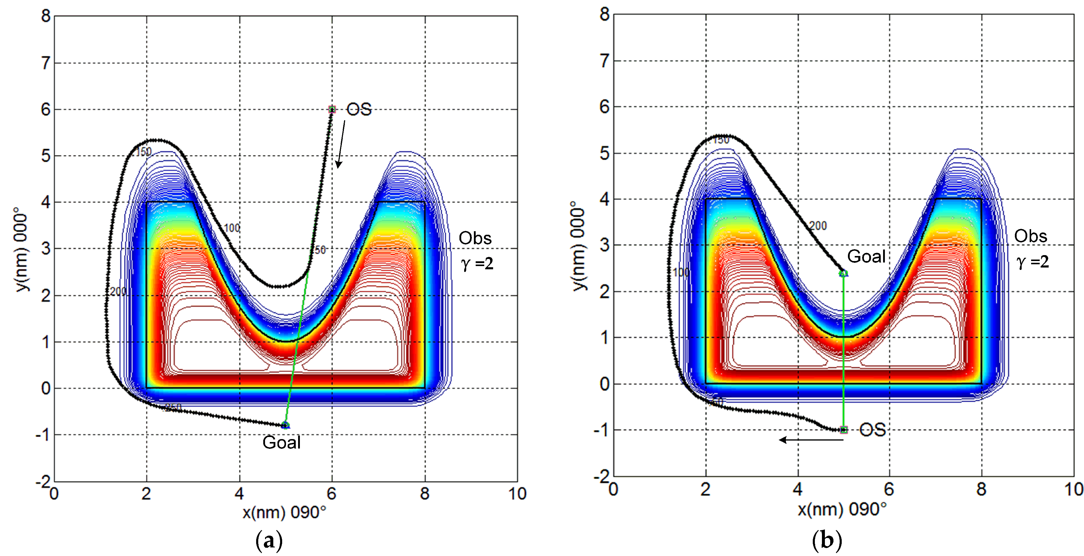
Figure 11.
The static obstacle is a U-shaped slot, a composite potential field composed of a parabola and a rectangle, where the parabola c is expressed as 3x2 − 30x + 79 − 4y. The boundary of this obstacle is indicated by the black lines. (a) The own ship is not trapped in the U-shaped slot and can successfully reach the goal, which is very close to the obstacle. (b) The goal is located inside the U-shaped slot and is very close to the obstacle; the own ship can still reach the goal.

Figure 12.
By adjusting the parameter γ of Obs3, the channel between Obs3 and Obs4 is navigable (when γ = 5) or unnavigable (when γ = 2). (a) The own ship detects that the potential between Obs3 and Obs4 is higher than the limited potential λ, that is, there are obstacles or non-navigable waters. Therefore, the own ship turns around the right side of Obs4 and finally reaches the goal near Obs5. (b) The own ship detects that the potential of the narrow channel between Obs3 and Obs4 is less than the limited potential value λ, which means the water is safe there. Therefore, the own ship passes through this narrow channel and reaches the goal safely.

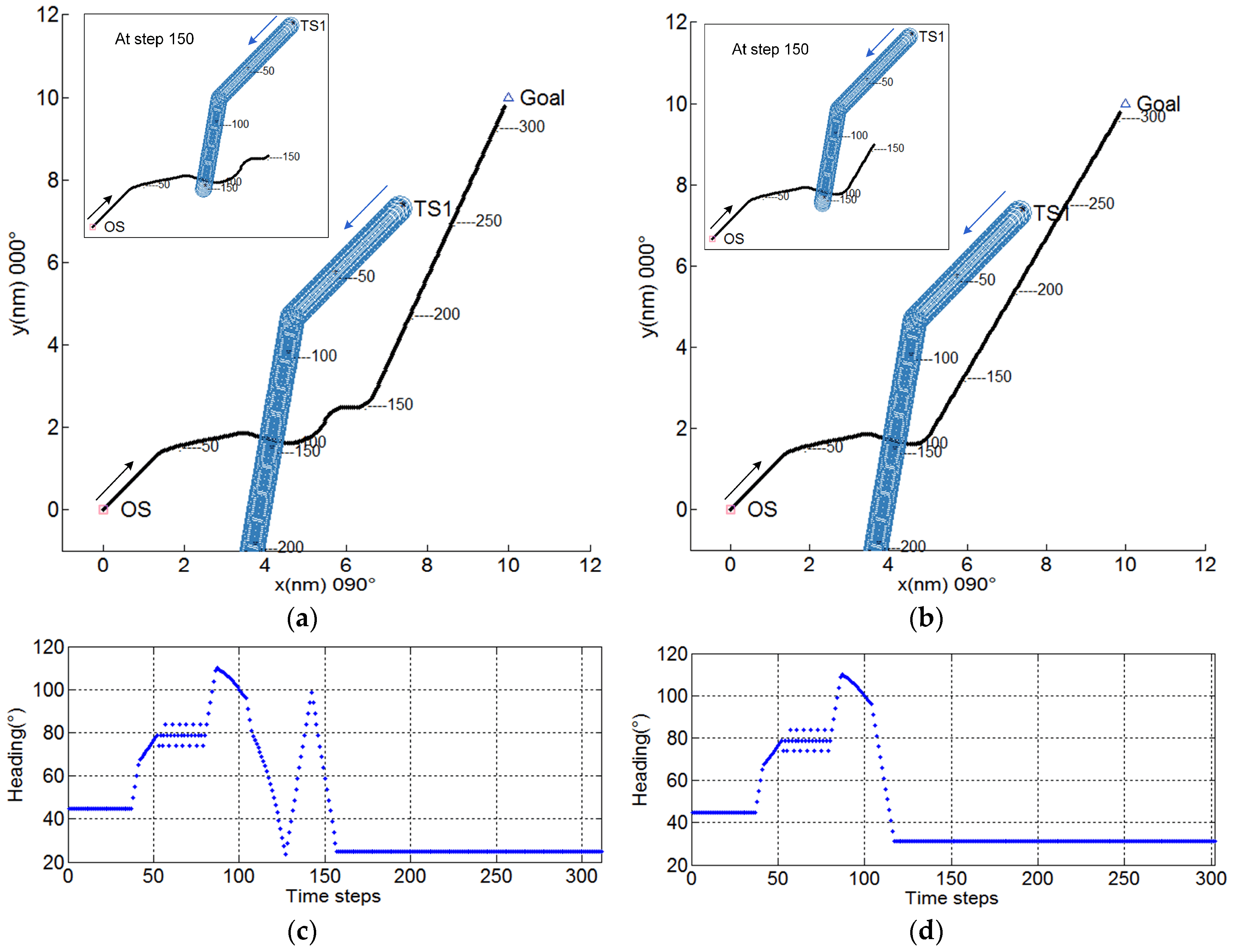
Figure 13.
Comparison of the simulations for two methods regarding emergency scenarios. (a) and (c) show the simulation results before the improvement, where the own ship can alter course 33° to starboard (at time step 37, range is more than 6 nm to TS1) and take a further 30° right turn when TS1 suddenly turns left 35° and heads toward the own ship (at time step 80). However, at time step 127, the own ship takes an extra right turn when there is no collision risk. The total distance of the own ship in this simulation is 15.5 nm with 311 time steps. (b) and (d) show the simulation results of the improved algorithm. Before time step 89, the actions of the own ship are consistent with the original algorithm. However, based on the criteria of DCPA and TCPA, the own ship then determines that there is no collision risk with the TS1 and begins to head for the goal (at time step 89), reaching there without additional course alteration. The final trajectory is smoother than before, and the length is optimized to 15.1 nm within 302 time steps. The total running time of the two simulations is almost the same.

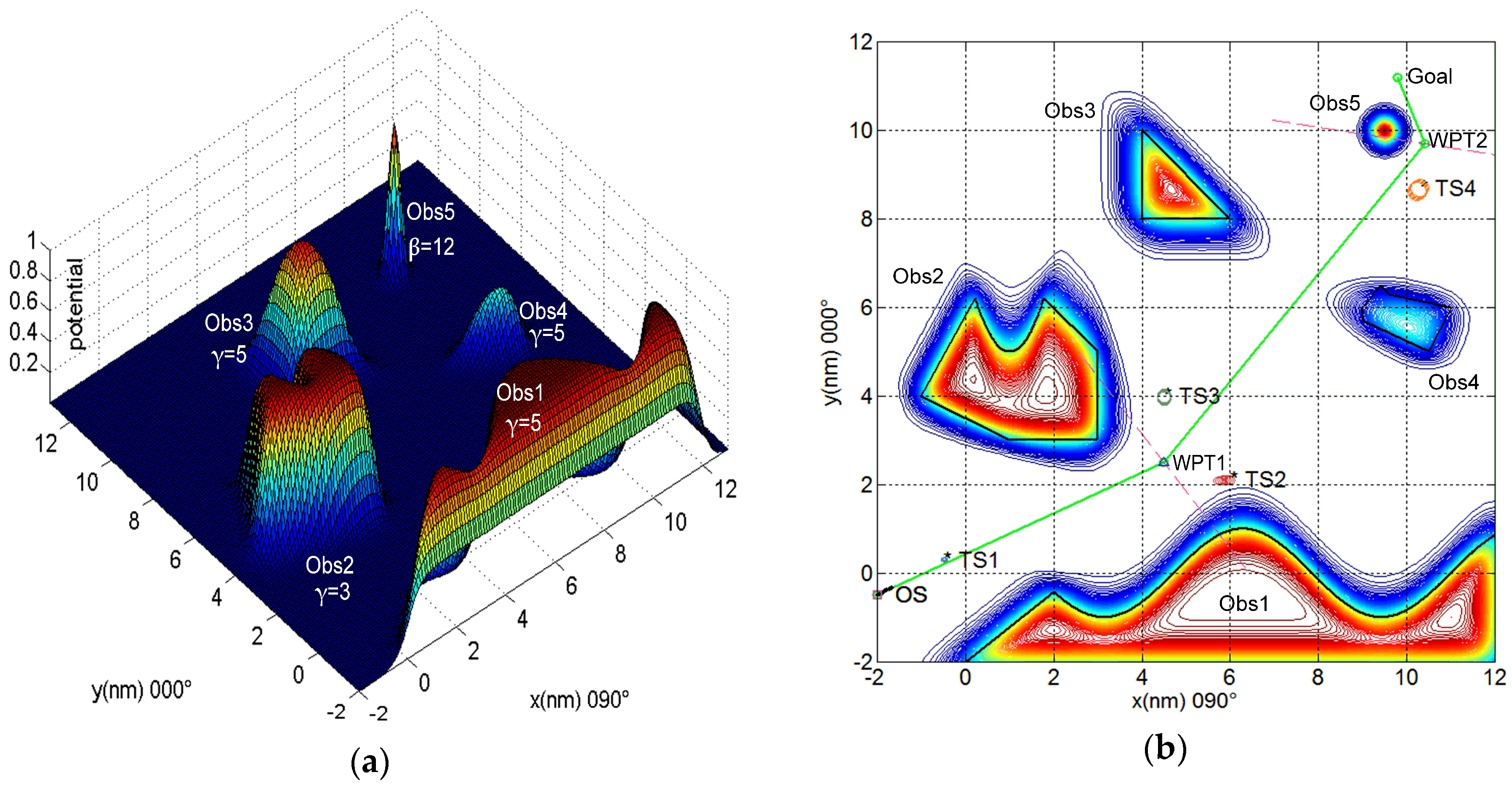
Figure 14.
(a) Three-dimensional potential field diagram of all static obstacle environments, including the parameter setting of each obstacle; (b) there is a low speed ship TS1 1.7 nm ahead of the own ship. The own ship, whose initial course is 060°, is coming up with TS1 from a direction more than 22.5° abaft the TS1’s beam, which is deemed an overtaking situation. The own ship should keep clear of TS1 and take account of the influences of Obs1, Obs2 and TS2 in this narrow channel.

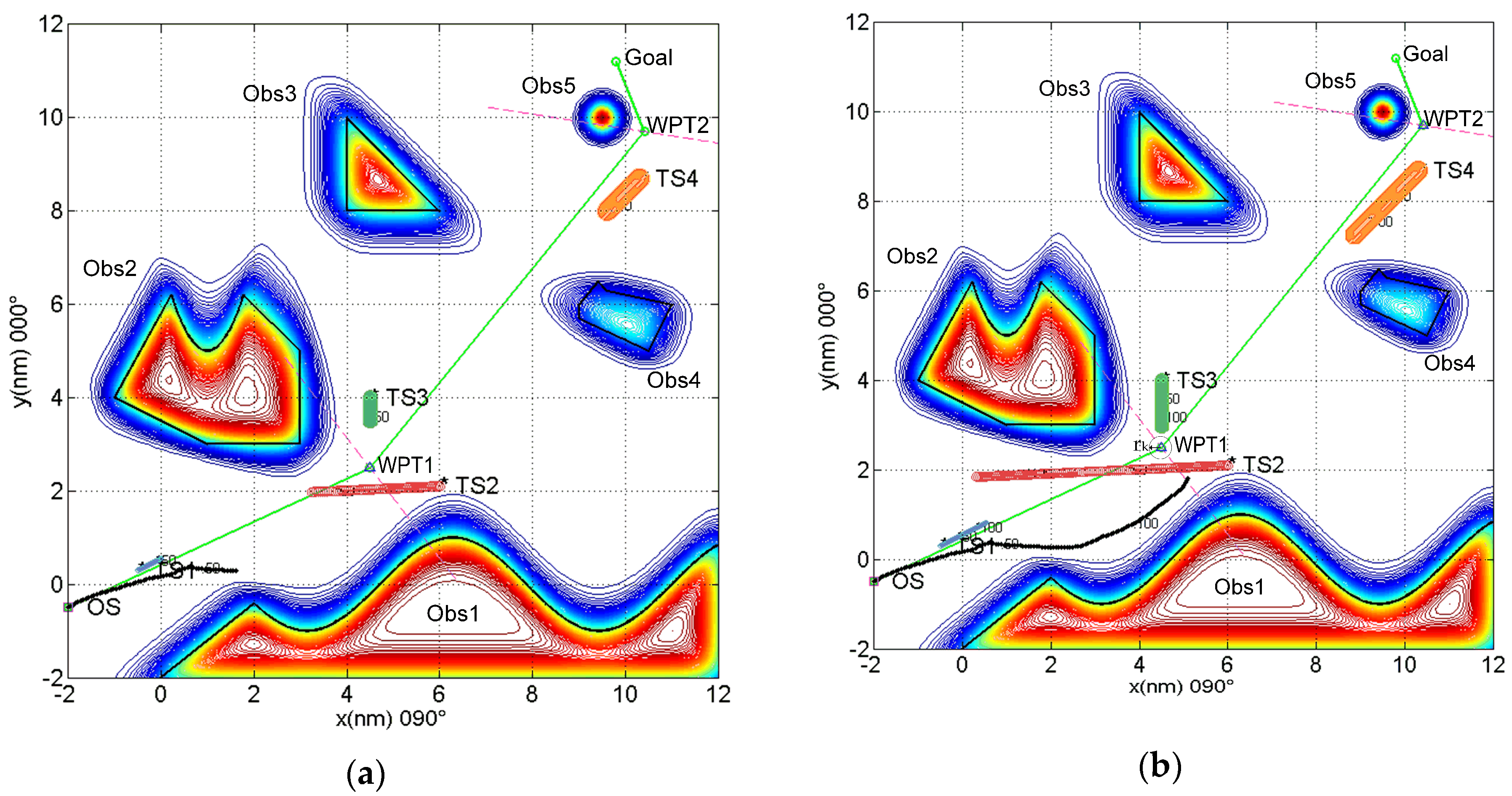
Figure 15.
(a) The own ship takes a right turn 20° to starboard due to Obs1 to overtake and pass TS1 at a range of 0.3 nm. After that, the crossing situation with TS2 requires the own ship to give way, so that the own ship alters course 30° to starboard and passes clear Obs1 by at least 0.7 nm. (b) TS2 has been passed clear at a range of 1.6 nm. Without the influence of TS3, the own ship would alter course to port to approach WPT1 due to the large distance between the own ship and WPT1 (more than rk), but doing this could go against Rules 15 & 17 of COLREGS and cause immediate danger with TS3. Therefore, the own ship keeps course not to port and not further to starboard due to the existence of the area obstacle Obs1 on the starboard side and passes TS3 at a safe distance of approximately 1.0 nm. Finally, the own ship crosses the angular bisector composed of the successive path legs and approaches the next waypoint WPT2.

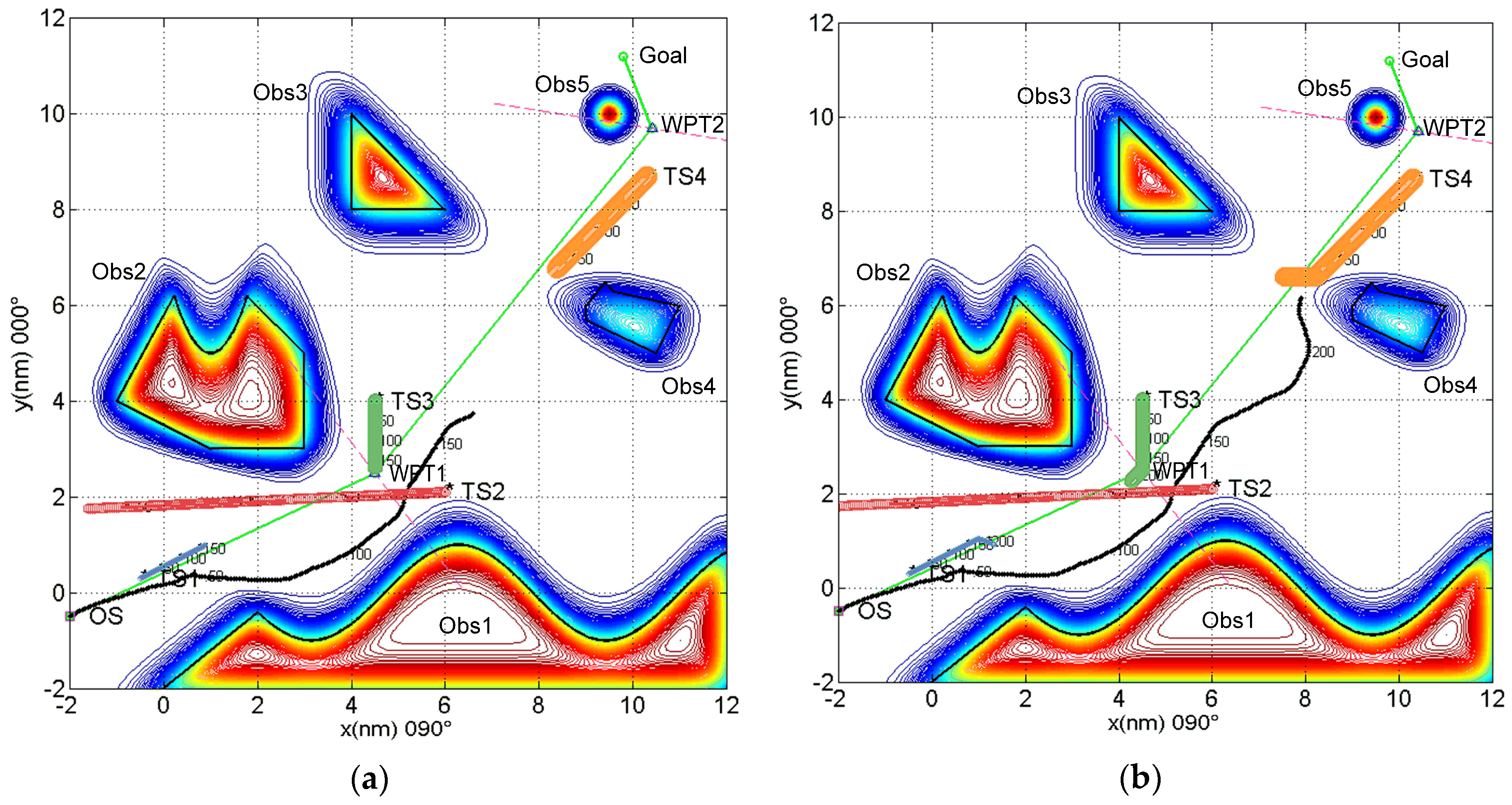
Figure 16.
(a) When heading to WPT2, the own ship encounters TS4 in a head-on situation. It is noted that TS4 does not alter her course to starboard; hence, in the range of 4.6 nm to TS4, the own ship takes a substantial right turn 35° to pass on the port side of TS4. (b) The own ship takes a new course 065°, but there is a static obstacle Obs4 in front of her. Therefore, the own ship must avoid Obs4 and consider the influence of TS4. Finally, the own ship selects an optimal course to port and passes abaft the TS4 at a range of 0.6 nm due to the sudden course change 45° to starboard by TS4. In addition, the passing distance between the own ship and Obs4 is safe, approximately 1.0 nm.

Figure 17.
(a) After clearing Obs4 and TS4, the own ship heads for WPT2 and then reaches WPT2 and the final goal. Although the goal is very close to Obs5, the own ship can still reach the goal and keep a safe passing distance of 0.57 nm from the point obstacle Obs5. (b) The above figure shows the distance between the own ship and each TS at every time step. The below figure shows the heading changes of the own ship at each time step, where −50° means 310° in circular notation. Although the heading angle of the own ship has some small fluctuations, the trajectory direction reflects substantial alterations of course when avoiding TSs, which is in line with Rule 16 of COLREGS.

Figure 18.
Real-time maneuvering data obtained by a PD controller. (a) Own ship yaw angle, i.e., the heading at every second. This data curve is consistent with the heading data of the algorithm at each step. (b) This diagram reflects the change of the own ship speed (m/s) during the path planning. There is a small decrease in the velocity at each turn, which is consistent with the actual situation. (c) This diagram shows that the yaw rate is limited to ±0.5°/s. (d) The rudder angle of each turn does not exceed the starboard or port rudder of 15°.

Figure 19.
Comparison of dynamic path planning results for different values of rk with or without the angular bisector method. (a) rk = 0.25 nm without using the angular bisector method; (b) rk = 0.5 nm without using the angular bisector method; and (c) rk = 0.25 nm using the angular bisector method.


Table 1.
Comparison among different selected path planning methods and the authors’ method; artificial potential field (APF); bacterial potential field (BPF); APF-stochastic reachable (APF-SR); scalar potential surface (SPS); path-guided hybrid artificial potential field (PGHAPF).
Table 1.
Comparison among different selected path planning methods and the authors’ method; artificial potential field (APF); bacterial potential field (BPF); APF-stochastic reachable (APF-SR); scalar potential surface (SPS); path-guided hybrid artificial potential field (PGHAPF).
| Methods | Lee 2004 APF [6] | Xue 2011 APF [12] | Montiel 2015 BPF [15] | Chiang 2015 APF-SR [10] | Liu 2018 APF [14] | Bayat 2018 SPS [16] | PGHAPF This Paper |
|---|---|---|---|---|---|---|---|
| International Regulations for Preventing Collisions at Sea (COLREGS) compliance | medium | medium | N/A | N/A | N/A | N/A | high |
| Map type | grid | grid | grid | grid | image | image | grid |
| Shape of obstacles | circle | polygon 1 | circle | square | arbitrary | arbitrary | arbitrary |
| Static obstacles | 1 | multi | 2–6 | 300 | multi | multi | multi |
| Dynamic obstacles | 1 | 1–5 | 1 | 300 | no | 2 | multi |
| Dynamic properties | yes | yes | no | no | no | yes | yes |
| Emergency collision avoidance (CA) actions | no | no | yes | yes | no | yes | yes |
| Computational time | high | ? | medium | low | medium | very low | very low |
| Local minima | ? | E | O | O | O | O | O |
| Goals non-reachable with obstacles nearby (GNRON) | ? | E | O | E | ? | O | O |
| Potential (P) or gradient (G) | G | G | G | G | G | P | P&G |
1 the polygons are constructed by many circles. O: this problem can be overcome, E: this problem still exists.
Table 2.
Spatial vector data in the electronic navigational chart (ENC).
| Vector Format | Represented Obstacles (Including but not Limited to) |
|---|---|
| point | isolated reefs, wrecks, navigational aids, etc. |
| curve (line) | safety contours, channel limits, etc. |
| surface (face) | boundaries of bigger obstacles, other natural and cultural areas, etc. |
Table 3.
Suggested configuration of the parameters β and γ for different spatial objects.
| Spatial Objects | Features | Distance (nm) | Parameter |
|---|---|---|---|
| point | wrecks, reefs | >2 | β < 1 |
| aids to navigation | >0.5 | β < 10 | |
| curve | safety contours channel limits | >1 | γ < 3 |
| channel limits | >0.2 | γ < 10 | |
| surface | islands, shoals | >3 | γ < 0.5 |
Table 4.
Ship particulars of Mariner class vessels.
| Description and Symbols | Value | Unit |
|---|---|---|
| Length overall (LOA) | 171.8 | m |
| Length between perpendiculars (LBP) | 160.93 | m |
| Maximum beam (B) | 23.17 | m |
| Design draft (T) | 8.23 | m |
| Loaded displacement (D) | 18,541 | T |
| Design speed (U) | 15 | knots |
| Max. rudder angle (δ) | 35 | degree |
| Max. rudder rate () | 5 | degree/s |
Table 5.
Initial inputs and simulation results for U-shaped obstacles.
| Situation | Start | Initial Course [°] | Goal | Length of Trajectory [nm] | Time Steps | Run Time [s] |
|---|---|---|---|---|---|---|
| (a) | (6, 6) | 190 | (5, −0.8) | 18.22 | 293 | 0.490 |
| (b) | (5, −1) | 270 | (5, 2.4) | 13.49 | 219 | 0.387 |
Table 6.
Initial inputs for complex static obstacles.
| Situation | Obs3 | Start | Initial Course [°] | Goal | Length of Trajectory [nm] | Time Steps | Run Time [s] |
|---|---|---|---|---|---|---|---|
| (a) | γ = 2 | (−2, 0.5) | 060 | (9.8, 11.2) | 22.17 | 358 | 0.611 |
| (b) | γ = 5 | (−2, 0.5) | 060 | (9.8, 11.2) | 17.57 | 284 | 0.527 |
Table 7.
Initial inputs for the simulation of emergency scenarios.
| Ship | Start | Speed | Initial Course [°] | Goal |
|---|---|---|---|---|
| own ship | (0.0, 0.0) | 12.0 | 045 | (10, 10) |
| TS1 | (7.3, 7.3) | 11.3 | 225 | / |
Table 8.
Results comparison for the two methods.
| Method | Length of Trajectory [nm] | Time Steps | Run Time [s] |
|---|---|---|---|
| Original | 15.5 | 311 | 0.11–0.12 |
| New | 15.1 | 302 | 0.10–0.12 |
Table 9.
Initial inputs and simulation results for dynamic TSs in a complex environment.
| No. | pts | vts [kn] | Rts [nm] | Situation | Ranges to TS [nm] | Own Ship Alters Course to | DCPA [nm] |
|---|---|---|---|---|---|---|---|
| TS1 | (−0.5, 0.3) | (2, 1) | 0.05 | overtaken | 1.7 | starboard | 0.3 |
| TS2 | (6.0, 2.1) | (−11.0, −0.5) | 0.1 | crossing A | >4 | starboard | 1.6 |
| TS3 | (4.5, 4) | (0, −2) | 0.15 | crossing B | / | keep course | 1.0 |
| TS4 | (10.3, 8.7) | (−2.8, −2.8) | 0.2 | head-on | 4.6 | starboard | 0.6 |
Table 10.
Initial inputs and simulation results for U-shaped obstacles.
| No. | Static Obstacles | Dynamic TSs | Distance [nm] | Time Steps | Total Run Time [s] | Time of Each Time Step [ms] |
|---|---|---|---|---|---|---|
| 1 | 1 | 0 | 18.22 | 293 | 0.490 | 1.7 |
| 2 | 1 | 0 | 13.49 | 219 | 0.387 | 1.8 |
| 3 | 5 | 0 | 22.17 | 358 | 0.611 | 1.7 |
| 4 | 5 | 0 | 17.57 | 284 | 0.527 | 1.9 |
| 5 | 0 | 1 | 15.5 | 311 | 0.11–0.12 | 0.4 |
| 6 | 0 | 1 | 15.1 | 302 | 0.10–0.12 | 0.4 |
| 7 | 5 | 4 | 19.38 | 315 | 0.804–0.833 | 2.6 |
© 2018 by the authors. Licensee MDPI, Basel, Switzerland. This article is an open access article distributed under the terms and conditions of the Creative Commons Attribution (CC BY) license (http://creativecommons.org/licenses/by/4.0/).
Share and Cite
MDPI and ACS Style
Lyu, H.; Yin, Y. Fast Path Planning for Autonomous Ships in Restricted Waters. Appl. Sci. 2018, 8, 2592. https://doi.org/10.3390/app8122592
AMA Style
Lyu H, Yin Y. Fast Path Planning for Autonomous Ships in Restricted Waters. Applied Sciences. 2018; 8(12):2592. https://doi.org/10.3390/app8122592
Chicago/Turabian StyleLyu, Hongguang, and Yong Yin. 2018. "Fast Path Planning for Autonomous Ships in Restricted Waters" Applied Sciences 8, no. 12: 2592. https://doi.org/10.3390/app8122592
Note that from the first issue of 2016, this journal uses article numbers instead of page numbers. See further details here.